Collapsed heteroclinic snaking near a heteroclinic chain in dragged meniscus problems

Abstract

A liquid film is studied that is deposited onto a flat plate that is inclined at a constant angle to the horizontal and is extracted from a liquid bath at a constant speed. We analyse steady-state solutions of a long-wave evolution equation for the film thickness. Using centre manifold theory, we first obtain an asymptotic expansion of solutions in the bath region. The presence of an additional temperature gradient along the plate that induces a Marangoni shear stress significantly changes these expansions and leads to the presence of logarithmic terms that are absent otherwise. Next, we numerically obtain steady solutions and analyse their behaviour as the plate velocity is changed. We observe that the bifurcation curve exhibits collapsed (or exponential) heteroclinic snaking when the plate inclination angle is above a certain critical value. Otherwise, the bifurcation curve is monotonic. The steady profiles along these curves are characterised by a foot-like structure that is formed close to the meniscus and is preceded by a thin precursor film further up the plate. The length of the foot increases along the bifurcation curve. Finally, we prove with a Shilnikov-type method that the snaking behaviour of the bifurcation curves is caused by the existence of an infinite number of heteroclinic orbits close to a heteroclinic chain that connects in an appropriate three-dimensional phase space the fixed point corresponding to the precursor film with the fixed point corresponding to the foot and then with the fixed point corresponding to the bath.

1 Introduction

Spreading liquids on a surface by pulling a plate out of a liquid bath is a well known coating process used for industrial applications WeRu04 . In order to gain control over the coating process, this problem has been studied from an experimental point of view, see, e.g., refs. Morey40 ; Rossum1958 ; SpSuWi74 ; SADF07 ; DFSA08 ; Maleki2011a , and also theoretically, see, e.g., refs. SADF07 ; LaLe42 ; Groe70a ; Groe70b ; Wi81 ; ZiSnEg09 . Landau and Levich LaLe42 , for example, analysed liquid films of constant thickness coating a vertical plate extracted from a bath of liquid at low velocities and found that the film thickness scales as $U^{2/3}$, where $U$ is the velocity of the plate. The asymptotic result of Landau and Levich was improved by Wilson Wi81 . Non-Landau-Levich-type solutions, which satisfy other scaling laws, were also found, see, for example, refs. SADF07 ; BCM10 ; JiAcMu05 ; Snoe08 ; ME05 . In particular, multiple non-Landau-Levich type solutions were previously observed by Münch et al. ME05 for certain parameter values in a similar system, where the role of the plate withdrawal is taken by a Marangoni shearing induced by a constant temperature gradient on the plate. Related behaviour is also found in coating problems involving complex fluids. A particular example is the deposition of line patterns in the process of Langmuir-Blodgett transfer of a surfactant layer from a bath onto a moving plate RiSp1992tsf ; KGFC10 . For this system a reduced Cahn-Hilliard type model was employed to show that the deposition of lines is related to local and global bifurcations of time-periodic states from a snaking bifurcation curve of steady-state front solutions KGFT12 , that in the light of the present work may be seen as a case of heteroclinic snaking (also cf. review Thie14 where this is set into the wider context of deposition patterns).

Table 1: Hierarchy of systems exhibiting collapsed (or exponential) snaking behaviour.

Authors	Description of scenario	$\#$ Fixed Points
Shilnikov Shil65	infinite number of periodic orbits	1 fixed point
Glendinning & Sparrow GlSp1984jsp	approaching a homocline
J. Knobloch $\&$ Wagenknecht KnoWa05	infinite number of homoclines	2 fixed points
Ma, Burke & E. Knobloch MaBK2010pd	approaching a hetereoclinic cycle
Present study	infinite number of heteroclines	3 fixed points
	approaching a hetereoclinic chain

In the present study, we do not consider Landau-Levich solutions where the thick drawn film directly connects to the meniscus of the bath. Instead we focus on a different type of film profiles which show a foot-like structure of characteristic thickness $h_{f}$ close to the meniscus that is preceded by a very thin precursor film of characteristic thickness $h_{p}$ further up the plate. They were recently described for a slip model SADF07 ; ZiSnEg09 . We show that for the precursor film model (as known in case of the slip model) at inclination angles $\alpha$ below a critical value $\alpha_{c}$, the foot shape is monotonic while for $\alpha>\alpha_{c}$ there exist undulations on top of the foot. In both cases we observe that for each inclination angle foot solutions exist when the plate velocity is close to a certain limiting velocity, and the closer the bifurcation curve approaches this limiting value, the larger the foot length becomes. The analysis of the bifurcation diagrams of foot solutions for a suitable solution measure, shows that this classical physico-chemical problem turns out to be a rich example to illustrate collapsed (or exponential) heteroclinic snaking near a hetereoclinic chain noteSnaking . We demonstrate that the three regions of the liquid film profile, namely, the precursor film, the foot and the bath, can be considered as three fixed points $\boldsymbol{y}_{p}$, $\boldsymbol{y}_{f}$ and $\boldsymbol{y}_{b}$ of an appropriate three-dimensional dynamical system. The steady film profiles are then described by heteroclinic orbits connecting points $\boldsymbol{y}_{p}$ and $\boldsymbol{y}_{b}$. Then, we show that the collapsed heteroclinic snaking observed in the dragged meniscus problem is caused by a perturbation of a heteroclinic chain that connects $\boldsymbol{y}_{p}$ with $\boldsymbol{y}_{f}$ and $\boldsymbol{y}_{f}$ with $\boldsymbol{y}_{b}$ that exists for certain parameter values, provided that fixed points $\boldsymbol{y}_{p}$ and $\boldsymbol{y}_{b}$ have two-dimensional unstable and two-dimensional stable manifolds, respectively, and that the fixed point $\boldsymbol{y}_{f}$ is a saddle focus with a one-dimensional stable manifold and a two-dimensional unstable manifold.

Note that related collapsed snaking behaviour has been analysed in systems involving either one fixed point Shil65 ; Shil67 ; GlSp1984jsp or two fixed points KnoWa05 ; MaBK2010pd . Table 1 illustrates that our results form part of a hierarchy of such snaking behaviours: Shilnikov (see refs. Shil65 ; Shil67 ) analyses homoclinic orbits to saddle-focus fixed points in three-dimensional dynamical systems that exist for some value $\beta_{0}$ of a parameter $\beta$ and demonstrated that if the fixed point has a one-dimensional unstable manifold and a two dimensional stable manifold, so that the eigenvalues of the Jacobian at this point are $\lambda_{1}$ and $-\lambda_{2}\pm\mathrm{i}\>\omega,$ where $\lambda_{1,2}$ and $\omega$ are positive real numbers, and if the saddle index $\delta\equiv\lambda_{2}/\lambda_{1}<1$, then in the neighbourhood of the primary homoclinic orbit there exists an infinite number of periodic orbits that pass near the fixed point several times. Moreover, the difference in the periods of these orbit tends asymptotically to $\pi/\omega$. The perturbation of the structurally unstable homoclinic orbit leads to a snaking bifurcation diagram showing the dependence of the period of the orbit versus the bifurcation parameter $\beta$. This diagram has an infinite but countable number of turning points at which the periodic orbits vanish in saddle-node bifurcations. However, if the saddle index is greater than unity, then the bifurcation diagram is monotonic. Knobloch and Wagenknecht KnoWa05 ; KnoWa08 analyse symmetric heteroclinic cycles connecting saddle-focus equilibria in reversible four-dimensional dynamical systems that arise in a number of applications, e.g., in models for water waves in horizontal water channels Che00 and in the study of cellular buckling in structural mechanics Hun00 . In these systems the symmetric heteroclinic cycle organises the dynamics in an equivalent way to the homoclinic solution in Shilnikov’s case. It is found that a necessary condition for collapsed snaking in such four-dimensional systems is the requirement that one of the involved fixed points is a bi-focus KnoWa05 . Then there exists an infinite number of homoclines to the second involved fixed point that all pass a close neighbourhood of the bi-focus. The presently studied case is equivalent to the cases of Shilnikov and of Knobloch and Wagenknecht, however, here a heteroclinic chain between three fixed points forms the organising centre of an infinite number of heteroclines.

The rest of the paper is organised as follows. In sect. 2, we introduce the model equation. In sect. 3, we analyse asymptotic behaviour of solutions in the bath region. In sect. 4 we present numerical results for the steady states and their snaking behaviour in the cases without and with Marangoni driving. Section 5 is devoted to an analytical explanation of the bifurcation diagrams obtained in sect. 4. Finally, in sect. 6 we present our conclusions.

2 Model equation

We consider a flat plate that forms a constant angle with the horizontal direction and that is being withdrawn from a pool of liquid at a constant speed. A schematic representation of the system is shown in fig. 1. We introduce a Cartesian coordinate system $(x,\,z)$ with the $x$-axis pointing downwards along the plate and the $z$-axis pointing upwards and being perpendicular to the plate. We assume that the free surface is two-dimensional, with no variations in the transverse direction. The position of the free surface is given by the equation $z=h(x,\,t)$, where $t$ denotes time. As a model equation governing the evolution of the free surface, we use a long-wave equation derived in refs. ODB97 ; Thie07 from the Navier-Stokes equations and the corresponding boundary conditions under the assumptions that the physical plate inclination angle is small and the typical longitudinal length scale of free-surface variations is large compared to the typical film thickness:

$$\partial_{t}h = -\partial_{x}\biggl{(}\frac{h^{3}}{3}\partial_{x}[\partial_{x}^{2}h+\Pi(h)]$$ (1)

$$\qquad\qquad-\frac{h^{3}}{3}G(\partial_{x}h-\alpha)-\frac{U}{3}h\biggr{)}.$$

Here $\alpha$, $U$ and $G$ are the scaled inclination angle of the plate, the scaled plate velocity and the scaled gravity, respectively, and the symbols $\partial_{t}$ and $\partial_{x}$ denote partial differentiation with respect to $t$ and $x$, respectively. Note that the scaled angle $\alpha$ as well as the scaled equilibrium contact angle are $O(1)$ quantities. On the right-hand side, $-\partial_{x}^{2}h$ represents the Laplace pressure, $\Pi(h)$ represents the Derjaguin or disjoining pressure (that we will discuss in detail below), the term $G\partial_{x}h$ is due to the hydrostatic-pressure, $-G\alpha$ is due to the $x$-component of gravity and the last term is due to the drag of the plate.

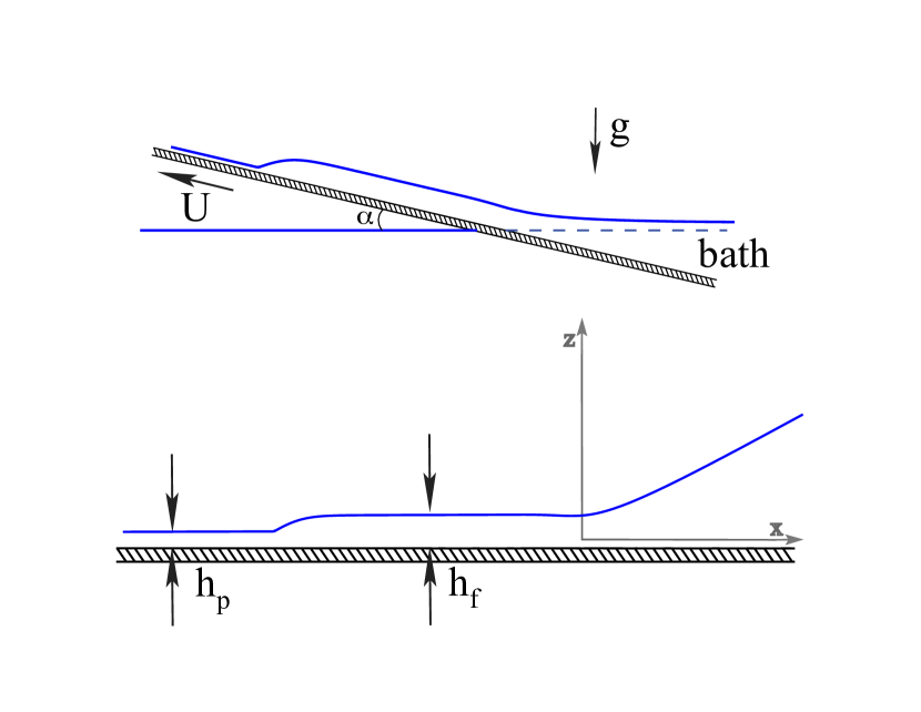
Figure 1: Sketch of the problem: Upper panel: An infinitely extended flat plate inclined at an angle $\alpha$ is withdrawn at a constant speed $U$ from a bath of a partially wetting liquid. Lower panel: Definition of the precursor film height, $h_{p}$, and the foot film height, $h_{f}$, for a typical film profile.

The interaction between the plate and the non-volatile partially wetting liquid is modelled via the disjoining pressure, which has the dimensional form

$$\widetilde{\Pi}(\tilde{h})=\widetilde{\Pi}_{1}(\tilde{h})+\widetilde{\Pi}_{2}(\tilde{h})=-\frac{A}{\tilde{h}^{3}}+\frac{B}{\tilde{h}^{6}}$$ (2)

consisting of a destabilising long-range van der Waals interaction, $\widetilde{\Pi}_{1}(\tilde{h})=-A/\tilde{h}^{3}$ , and a stabilising short-range interaction, $\widetilde{\Pi}_{2}(\tilde{h})=B/\tilde{h}^{6}$. Here $\tilde{h}$ is the dimensional film thickness, and $A$ and $B$ are the Hamaker constants. For $A$ and $B$ positive, on a horizontal plane the disjoining pressure describes partial wetting and characterises a stable precursor film of thickness

$$h_{\mathrm{eq}}=(B/A)^{1/3}$$ (3)

that may coexist with a meniscus of finite contact angle

$$\theta_{\mathrm{eq}}=\sqrt{\frac{3}{5}\frac{A}{\gamma h^{2}_{\mathrm{eq}}}},$$ (4)

where $\gamma$ is the surface tension coefficient (see refs. Thie07 ; deGe85 ; StVe09 ; Thie10 for background information and details).

Equation (1) has been non-dimensionalised using $\ell=\sqrt{3/5}\>h_{\mathrm{eq}}/\theta_{\mathrm{eq}}$ as the length scale in the $x$-direction, $h_{\mathrm{eq}}$ as the length scale in the $z$-direction and $\tau\!\!=\!\!(9\eta h_{\mathrm{eq}})/(25\gamma\theta^{4}_{\mathrm{eq}})$ as the time scale, where $\eta$ is the viscosity of the liquid. Note that with this non-dimensionalisation the dimensionless disjoining pressure has the form

$${\Pi}(h)={\Pi}_{1}(h)+{\Pi}_{2}(h)=-\frac{1}{h^{3}}+\frac{1}{h^{6}}.$$ (5)

The scaled velocity, gravity number and the inclination angle are given by

$$U=\frac{3\tau}{\ell}u,\quad G=\frac{\rho gh_{\mathrm{eq}}^{4}}{A},\quad\alpha=\frac{\ell}{h_{\mathrm{eq}}}\tilde{\alpha},$$ (6)

respectively, where $\rho$ is the density of the liquid and $g$ is gravity and $u$ and $\tilde{\alpha}$ are the dimensional plate velocity and the plate inclination angle, respectively.

Note that additional physical effects can be included into the model presented above. One extension that is interesting for reasons that will become clear later, is the inclusion of a term quadratic in $h$ in the flux on the right-hand side of eq. (1). This can be obtained, for example, by assuming that there is an additional constant temperature gradient along the plate, see refs. Cazabat1990 ; ME05 ; ScNiSt10 ; ScNiSt12 for more details. Inclusion of this effect into the present model results in

$$\partial_{t}h = -\partial_{x}\biggl{(}\frac{h^{3}}{3}\partial_{x}[\partial_{x}^{2}h+\Pi(h)]$$ (7)

$$\qquad-\frac{h^{3}}{3}G(\partial_{x}h-\alpha)-\frac{\Omega}{3}h^{2}-\frac{U}{3}h\biggr{)},$$

where $\Omega$ is a dimensionless number representing the temperature gradient along the plate.

Finally, we discuss boundary conditions. First, we assume that $h$ tends to an undetermined constant value (e.g., at equilibrium the precursor film thickness) as $x\rightarrow-\infty$ and its derivatives tend to zero as $x\rightarrow-\infty$. Second, we assume that $h_{x}=\alpha+o(1)$ as $x\rightarrow\infty$, which means that the slope of the free surface of the bath approaches the horizontal direction far away from the plate. The asymptotic behaviour of $h$ as $x\rightarrow\infty$ will be analysed in more detail in the next section.

3 Asymptotic behaviour of solutions at infinity

In what follows, we will analyse steady-state solutions of eq. (7), i.e., solutions that satisfy the equation

$$h^{3}[h^{\prime\prime}+\Pi(h)]^{\prime}-Gh^{3}(h^{\prime}-\alpha)-\Omega h^{2}-Uh+C_{0}=0,$$ (8)

where now $h$ is a function of $x$ only and primes denote differentiation with respect to $x$. Here, $C_{0}$ is a constant of integration and represents the flux. Note that $C_{0}$ is in fact not an independent parameter but is determined as part of the solution of the boundary-value problem consisting of eq. (8) and four boundary conditions that will be discussed in the next section.

Following a proposal of ref. ME05 , we introduce variables $y_{1}=1/h$, $y_{2}=h^{\prime}$ and $y_{3}=h^{\prime\prime}$, and convert the steady-state equation (8) into a three-dimensional dynamical system:

$$y_{1}^{\prime} = -y_{1}^{2}y_{2},$$ (9)

$$y_{2}^{\prime} = y_{3},$$ (10)

$$y_{3}^{\prime} = (6y_{1}^{7}-3y_{1}^{4})y_{2}+Gy_{2}+Uy_{1}^{2}$$ (11)

$$+\Omega y_{1}-C_{0}y_{1}^{3}-G\alpha.$$

Note that the transformation $y_{1}=1/h$ is used to obtain a new fixed point corresponding to the bath, namely the point $\boldsymbol{y}_{b}=(0,\,\alpha,\,0)$, beside other fixed points, two of which, $\boldsymbol{y}_{f}=(1/h_{f},\,0,\,0)$ and $\boldsymbol{y}_{p}=(1/h_{p},\,0,\,0)$, correspond to the foot and the precursor film, respectively. For a more detailed analysis of the fixed points, see the beginning of sect. 5.

To analyse the stability of the fixed point $\boldsymbol{y_{b}}$, we first compute the Jacobian at this point:

$$\boldsymbol{J}_{\boldsymbol{y}_{b}}=\left(\begin{array}[]{ccc}0&0&0\\ 0&0&1\\ \Omega&G&0\end{array}\right).$$ (12)

The eigenvalues are $0$, $\pm G^{1/2}$ and the corresponding eigenvectors are $(G,\,-\Omega,\,0)$, $(0,\,\pm G^{-1/2},\,1)$. So there is a one-dimensional centre (or critical) eigenspace, a one-dimensional stable eigenspace and a one-dimensional unstable eigenspace given by

$$T^{c}_{\boldsymbol{y}_{b}} = \mathrm{span}\{(G,\,-\Omega,\,0)\},$$ (13)

$$T^{s}_{\boldsymbol{y}_{b}} = \mathrm{span}\{(0,\,-G^{-1/2},\,1)\},$$ (14)

$$T^{u}_{\boldsymbol{y}_{b}} = \mathrm{span}\{(0,\,G^{-1/2},\,1)\},$$ (15)

respectively.

To determine the asymptotic behaviour of $h$ as $x\rightarrow\infty$, we analyse the centre manifold of $\boldsymbol{y}_{b}$, which we denote by $W^{c}_{\boldsymbol{y}_{b}}$. This is an invariant manifold whose tangent space at $\boldsymbol{y}_{b}$ is $T^{c}_{\boldsymbol{y}_{b}}$. The existence of a centre manifold is provided by the centre manifold theorem (see, e.g., theorem 1, p. 4 in ref. Carr_1981 , theorem 5.1, p. 152 in ref. Kuz98 ). For simplicity, we use the substitution $z_{1}=y_{1}$, $z_{2}=y_{2}-\alpha$, $z_{3}=y_{3}$. In vector notation, the dynamical system takes the form

$$\boldsymbol{z}^{\prime}=\boldsymbol{f}(\boldsymbol{z}),$$ (16)

where $\boldsymbol{f}(\boldsymbol{z})=(f_{1}(\boldsymbol{z}),\,f_{2}(\boldsymbol{z}),\,f_{3}(\boldsymbol{z}))^{T}$ and

$$\!\!\!\!\!\!f_{1}(\boldsymbol{z})=f_{1}(z_{1},\,z_{2},\,z_{3}) = -z_{1}^{2}(z_{2}+\alpha),$$ (17)

$$\!\!\!\!\!\!f_{2}(\boldsymbol{z})=f_{2}(z_{1},\,z_{2},\,z_{3}) = z_{3},$$ (18)

$$\!\!\!\!\!\!f_{3}(\boldsymbol{z})=f_{3}(z_{1},\,z_{2},\,z_{3}) = (6z_{1}^{7}-3z_{1}^{4})(z_{2}+\alpha)+Gz_{2}$$ (19)

$$+Uz_{1}^{2}+\Omega z_{1}-C_{0}z_{1}^{3}.$$

The fixed point corresponding to the bath is then $\boldsymbol{z}_{b}=(0,\,0,\,0)$. Next, we rewrite the system of ordinary differential equations (16) in its eigenbasis at $\boldsymbol{z}_{b}$, i.e., we use the change of variables $\boldsymbol{u}=\boldsymbol{B}^{-1}\boldsymbol{z}$, where $\boldsymbol{B}$ is the matrix having the eigenvectors of the Jacobian as its columns,

$$\boldsymbol{B}=\left(\begin{array}[]{ccc}G&0&0\\ -\Omega&G^{-1/2}&-G^{-1/2}\\ 0&1&1\end{array}\right),$$ (20)

and obtain the system

$$\boldsymbol{u}^{\prime}=\boldsymbol{g}(\boldsymbol{u})\equiv\boldsymbol{B}^{-1}\boldsymbol{f}(\boldsymbol{B}\boldsymbol{u}),$$ (21)

which can be written in the form

$$\xi^{\prime}=\psi(\xi,\boldsymbol{\eta}),$$ (22)

$$\boldsymbol{\eta}^{\prime}=\boldsymbol{C}\boldsymbol{\eta}+\boldsymbol{\varphi}(\xi,\boldsymbol{\eta}),$$ (23)

where $\xi$ denotes the first component of $\boldsymbol{u}$ and $\boldsymbol{\eta}=(\eta_{1},\,\eta_{2})^{T}$ consist of the second and the third components of $\boldsymbol{u}$ (i.e., $\xi\equiv u_{1}$, $\eta_{1}\equiv u_{2}$ and $\eta_{2}\equiv u_{3}$), $\psi$ and $\boldsymbol{\varphi}$ have Taylor expansions that start with quadratic or even higher order terms and $\boldsymbol{C}$ is the matrix

$$\boldsymbol{C}=\left(\begin{array}[]{cc}G^{1/2}&0\\ 0&-G^{1/2}\end{array}\right).$$ (24)

After some algebra, we find

$$\psi(\xi,\boldsymbol{\eta}) = G{\Omega}\xi^{3}-G{\alpha}\xi^{2}-G^{1/2}\xi^{2}\eta_{1}+G^{1/2}\xi^{2}\eta_{2},$$ (25)

$$\varphi_{1}(\xi,\boldsymbol{\eta}) = -3\,{G}^{7}\Omega\,{\xi}^{8}+3\,{G}^{7}\alpha\,{\xi}^{7}+3\,{G}^{13/2}{\xi}^{7}\eta_{1}$$ (26)

$$-3\,{G}^{13/2}{\xi}^{7}\eta_{2}+\frac{3}{2}\,{G}^{4}\Omega\,{\xi}^{5}-\frac{3}{2}\,{G}^{4}\alpha\,{\xi}^{4}$$

$$-\frac{3}{2}\,{G}^{7/2}{\xi}^{4}\eta_{1}+\frac{3}{2}\,{G}^{7/2}{\xi}^{4}\eta_{2}-\frac{1}{2}\,C_{0}\,{G}^{3}{\xi}^{3}$$

$$+\frac{1}{2}\,{G}^{3/2}\Omega^{2}{\xi}^{3}-\frac{1}{2}\,{G}^{3/2}\Omega\,\alpha\,{\xi}^{2}+\frac{1}{2}\,U{G}^{2}{\xi}^{2}$$

$$-\frac{1}{2}\,G\Omega\,{\xi}^{2}\eta_{1}+\frac{1}{2}\,G\Omega\,{\xi}^{2}\eta_{2},$$

$$\varphi_{2}(\xi,\boldsymbol{\eta}) = -{G}^{1/2}\eta_{2}-3\,{G}^{7}\Omega\,{\xi}^{8}+3\,{G}^{7}\alpha\,{\xi}^{7}$$ (27)

$$+3\,{G}^{13/2}{\xi}^{7}\eta_{1}-3\,{G}^{13/2}{\xi}^{7}\eta_{2}+\frac{3}{2}\,{G}^{4}\Omega\,{\xi}^{5}$$

$$-\frac{3}{2}\,{G}^{4}\alpha\,{\xi}^{4}-\frac{3}{2}\,{G}^{7/2}{\xi}^{4}\eta_{1}+\frac{3}{2}\,{G}^{7/2}{\xi}^{4}\eta_{2}$$

$$-\frac{1}{2}\,{C_{0}}\,{G}^{3}{\xi}^{3}-\frac{1}{2}\,{G}^{3/2}\Omega^{2}{\xi}^{3}+\frac{1}{2}\,{G}^{3/2}\Omega\,\alpha\,{\xi}^{2}$$

$$+\frac{1}{2}\,U{G}^{2}{\xi}^{2}+\frac{1}{2}\,G\Omega\,{\xi}^{2}\eta_{1}-\frac{1}{2}\,G\Omega\,{\xi}^{2}\eta_{2}.$$

Near the origin, $\boldsymbol{z_{b}}$, when $|\xi|<\delta$ for some positive $\delta$, the centre manifold in the $(\xi,\eta_{1},\eta_{2})$-space can be represented by the equations $\eta_{1}=g_{1}(\xi)$, $\eta_{2}=g_{2}(\xi)$, where $g_{1}$ and $g_{2}$ are in $C^{2}$. Moreover, near the origin system (22), (23) is topologically equivalent to the system

$$\xi^{\prime}=\psi(\xi,\boldsymbol{g}(\xi)),$$ (28)

$$\boldsymbol{\eta}^{\prime}=\boldsymbol{C}\boldsymbol{\eta}.$$ (29)

where the first equation represents the restriction of the flow to its centre manifold (see, e.g., theorem 1, p. 4 in ref. Carr_1981 , theorem 5.2, p. 155 in ref. Kuz98 ).

The centre manifold can be approximated to any degree of accuracy. According to theorem 3, p. 5 in ref. Carr_1981 , ‘test’ functions $\phi_{1}$ and $\phi_{2}$ approximate the centre manifold with accuracy $O(|\xi|^{q})$, namely,

$$|g_{1}(\xi)-\phi_{1}(\xi)|=O(|\xi|^{q}),\quad|g_{2}(\xi)-\phi_{2}(\xi)|=O(|\xi|^{q})$$ (30)

as $\xi\rightarrow 0$, provided that $\phi_{i}(0)=0$, $\phi_{i}^{\prime}(0)=0$, $i=1,\,2$ and $\boldsymbol{M}[\boldsymbol{\phi}](\xi)=O(|\xi|^{q})$ as $\xi\rightarrow 0$, where $\boldsymbol{M}$ is the operator defined by

$$\boldsymbol{M}[\boldsymbol{\phi}](\xi)=\boldsymbol{\phi}^{\prime}(\xi)\psi(\xi,\,\boldsymbol{\phi}(\xi))-\boldsymbol{C}\boldsymbol{\phi}(\xi)-\boldsymbol{\varphi}(\xi,\,\boldsymbol{\phi}(\xi)).$$ (31)

The centre manifold can now be obtained by seeking for $\phi_{1}(\xi)$ and $\phi_{2}(\xi)$ in the form of polynomials in $\xi$ and requiring that the coefficients of the expansion of $\boldsymbol{M}[\boldsymbol{\phi}](\xi)$ in Taylor series vanish at zeroth order, first order, second order, etc. Using this procedure, we can find the Taylor series expansions of $g_{1}$ and $g_{2}$:

$$g_{1}(\xi) \!\!\!=\!\!\! \left(\frac{1}{2}\,G\Omega\,\alpha-\frac{1}{2}\,{G}^{3/2}U\right)\xi^{2}$$ (32)

$$+\left({G}^{2}U\alpha-{G}^{3/2}\Omega\,{\alpha}^{2}-\frac{1}{2}\,G\Omega^{2}+\frac{1}{2}\,{G}^{5/2}C_{0}\right)\xi^{3}$$

$$-\biggl{(}\frac{3}{2}\,{G}^{3}\alpha\,C_{0}-3\,{G}^{2}{\alpha}^{3}\Omega+\frac{3}{2}\,{G}^{2}\Omega\,U-3\,{G}^{5/2}{\alpha}^{2}U$$

$$\qquad-\frac{3}{2}\,{G}^{7/2}\alpha-\frac{5}{2}\,{G}^{3/2}\alpha\,\Omega^{2}\biggr{)}\xi^{4}+\cdots,$$

$$g_{2}(\xi) \!\!\!=\!\!\! \left(\frac{1}{2}\,G\Omega\,\alpha+\frac{1}{2}\,{G}^{3/2}U\right)\xi^{2}$$ (33)

$$+\left({G}^{2}U\alpha+{G}^{3/2}\Omega\,{\alpha}^{2}-\frac{1}{2}\,G\Omega^{2}-\frac{1}{2}\,{G}^{5/2}C_{0}\right)\xi^{3}$$

$$-\biggl{(}\frac{3}{2}\,{G}^{3}\alpha\,C_{0}-3\,{G}^{2}{\alpha}^{3}\Omega-3\,{G}^{5/2}{\alpha}^{2}U+\frac{3}{2}\,{G}^{2}\Omega\,U$$

$$\qquad+\frac{3}{2}\,{G}^{7/2}\alpha+\frac{5}{2}\,{G}^{3/2}\alpha\,\Omega^{2}\biggr{)}\xi^{4}+\cdots.$$

Let $g_{i}^{(k)}(\xi)$, $i=1,\,2$, be the Taylor polynomial for $g_{i}(\xi)$ of degree $k$. Then $g_{i}(\xi)=g_{i}^{(k)}(\xi)+O(|\xi|^{k+1})$, $i=1,\,2$, and $\boldsymbol{M}[\boldsymbol{g}^{(k)}](\xi)=O(|\xi|^{k+1})$ as $\xi\rightarrow 0$. The dynamics on the centre manifold is therefore governed by the equation

$$\xi^{\prime} = \psi(\xi,\boldsymbol{g}^{(k)}(\xi))+O(|\xi|^{k+3})$$ (34)

$$= G{\Omega}\xi^{3}-G{\alpha}\xi^{2}-G^{1/2}\xi^{2}g_{1}^{(k)}(\xi)$$

$$+G^{1/2}\xi^{2}g_{2}^{(k)}(\xi)+O(|\xi|^{k+3}).$$

Substituting eq. (32) and eq. (33) into eq. (34), we find

$$\xi^{\prime} = -G\alpha\xi^{2}+G\Omega\xi^{3}+UG^{2}\xi^{4}-(C_{0}G^{3}-2G^{2}\Omega\alpha^{2})\xi^{5}$$ (35)

$$\qquad+(6G^{3}U\alpha^{2}-3G^{4}\alpha-5G^{2}\Omega^{2}\alpha)\xi^{6}+\cdots.$$

Taking into account the fact that $\xi=z_{1}/G$, we obtain

$$z_{1}^{\prime} =-\alpha z_{1}^{2}+\frac{\Omega}{G}z_{1}^{3}+\frac{U}{G}z_{1}^{4}-\biggl{(}\frac{C_{0}}{G}-\frac{2\Omega\alpha^{2}}{G^{2}}\biggr{)}z_{1}^{5}$$ (36)

$$+\biggl{(}\frac{6U\alpha^{2}}{G^{2}}-\frac{3\alpha}{G}-\frac{5\Omega^{2}\alpha}{G^{3}}\biggr{)}z_{1}^{6}+\cdots.$$

Rewriting this in terms of $h$, we get

$$h^{\prime} =\alpha-\frac{\Omega}{G}h^{-1}-\frac{U}{G}h^{-2}+\biggl{(}\frac{C_{0}}{G}-\frac{2\Omega\alpha^{2}}{G^{2}}\biggr{)}h^{-3}$$ (37)

$$\quad-\biggl{(}\frac{6U\alpha^{2}}{G^{2}}-\frac{3\alpha}{G}-\frac{5\Omega^{2}\alpha}{G^{3}}\biggr{)}h^{-4}+\cdots$$

as $h\rightarrow\infty$.

We seek for a solution for $h$ whose slope approaches that of the line corresponding to the horizontal direction as $x\rightarrow\infty$. In the chosen system of coordinates, the line corresponding to the horizontal direction has the slope $\alpha$. So we seek for a solution satisfying $h^{\prime}(x)=\alpha+o(1)$ as $x\rightarrow\infty$. This can also be written in the form

$$h(x)=\alpha x+o(x)\quad\text{as}\quad x\rightarrow\infty.$$ (38)

Substituting eq. (38) into eq. (37), we obtain

$$h^{\prime}=\alpha-\frac{\Omega}{\alpha G}x^{-1}+o(x^{-1}),$$ (39)

which implies

$$h=\alpha x-\frac{\Omega}{\alpha G}\log x+o(\log x).$$ (40)

Substituting eq. (40) into eq. (37), we find

$$h^{\prime}=\alpha-\frac{\Omega}{\alpha G}x^{-1}-\frac{\Omega^{2}}{\alpha^{3}G^{2}}x^{-2}\log x+o(x^{-2}\log x),$$ (41)

which implies

$$h=\alpha x-\frac{\Omega}{\alpha G}\log x+\frac{\Omega^{2}}{\alpha^{3}G^{2}}x^{-1}\log x+o(x^{-1}\log x).$$ (42)

In principle, any constant of integration can be added to this expression, and this reflects the fact that there is translational invariance in the problem, i.e., if $h(x)$ is a solution of eq. (8), then a profile obtained by shifting $h(x)$ along the $x$-axis is also a solution of this equation. Without loss of generality, we choose the constant of integration to be zero, which breaks this translational invariance and allows selecting a unique solution from the infinite set of solutions.

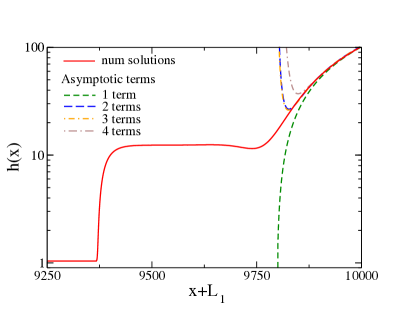
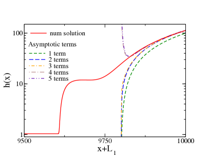
Figure 2: Left panel: Comparison between a numerical solution for $\Omega=0$ when $\alpha=0.5$ and $U=0.084$ and the expansion for $h(x)$ given by eq. (46) with 1-4 terms. Right panel: Comparison between a numerical solution for $\Omega=0.001$ when $\alpha=0.5$ at $U=0.076$ and the expansion for $h(x)$ given by eq. (45) with 1-5 terms. $L_{1}=9800$, $L_{2}=200$.

Substituting eq. (42) into eq. (37), we find

$$h^{\prime} = \alpha-\frac{\Omega}{\alpha G}x^{-1}-\frac{\Omega^{2}}{\alpha^{3}G^{2}}x^{-2}\log x$$ (43)

$$-\frac{U}{\alpha^{2}G}x^{-2}-\frac{\Omega^{3}}{\alpha^{5}G^{3}}x^{-3}\log^{2}x$$

$$+\frac{\Omega^{3}}{\alpha^{5}G^{3}}x^{-3}\log x+o(x^{-3}\log x),$$

which implies

$$h = \alpha x-\frac{\Omega}{\alpha G}\log x+\frac{\Omega^{2}}{\alpha^{3}G^{2}}x^{-1}\log x$$ (45)

$$+\biggl{(}\frac{\Omega^{2}}{\alpha^{3}G^{2}}+\frac{U}{\alpha^{2}G}\biggr{)}x^{-1}$$

$$-\frac{\Omega^{3}}{2\alpha^{5}G^{3}}x^{-2}\log^{2}x+o(x^{-2}\log x).$$

The procedure described above can be continued to obtain more terms in the asymptotic expansion of $h$ as $x\rightarrow\infty$. Note that all the terms in this expansion, except the first two, will be of the form $x^{-m}\log^{n}x$, where $m$ is a positive integer and $n$ is a non-negative integer. It should also be noted that the presence of the logarithmic terms in the asymptotic expansion of $h$ is wholly due to the quadratic contribution to the flux in eq. (7) that here results from a lateral temperature gradient. Without this term, i.e., for $\Omega=0$, the expansion (37) for $h^{\prime}$ does not contain the term proportional to $h^{-1}$. This implies that after substituting $h(x)=\alpha x+o(x)$ in this expansion, no term proportional to $x^{-1}$ will appear, and, therefore, integration will not lead to the appearance of a logarithmic term. In fact, it is straightforward to see that for $\Omega=0$ an appropriate ansatz for $h$ is

$$h\sim\alpha x+D_{1}x^{-1}+D_{2}x^{-2}+D_{3}x^{-3}+\cdots,$$ (46)

implying that

$$D_{1} = \frac{U}{\alpha^{2}G},\qquad D_{2}=-\frac{C_{0}}{2\alpha^{3}G},$$

$$D_{3} = -\frac{1}{3}\biggl{(}\frac{2U^{2}}{\alpha^{5}G}+\frac{3}{\alpha^{3}G}-\frac{6U}{\alpha^{2}G^{2}}\biggr{)},\,\,\ldots\,.$$ (47)

Note that the presence of a logarithmic term in the asymptotic behaviour of $h$ was also observed by Münch and Evans ME05 in a related problem of a liquid film driven out of a meniscus by a thermally induced Marangoni shear stress onto a nearly horizontal fixed plane. They find the following asymptotic behaviour of the solution, given with our definition of the coordinate system:

$$h(x)\sim h_{0}(x)+D_{0}+D_{1}\exp(-D^{1/2}x)\quad\text{as}\quad x\rightarrow\infty,$$ (48)

where $h_{0}=x/D-\log x+o(1)$, $D$ is the parameter measuring the relative importance of the normal component of gravity and $D_{0}$ and $D_{1}$ are arbitrary constants. The constant $D_{0}$ reflects the fact that there is translational invariance in the problem and it can be set to zero without loss of generality. An analysis performed along the lines indicated above shows that a more complete expansion has the form

$$h(x)\sim\frac{x}{D}-\log x+D\>x^{-1}\log x+D{x^{-1}}$$

$$+\frac{D^{2}}{2}x^{-2}\log^{2}x+\cdots.$$ (49)

Note that there is no need to include the exponentially small term as it is asymptotically smaller than all the other terms of the expansion.

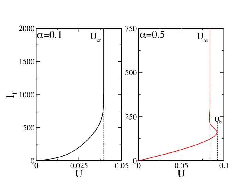
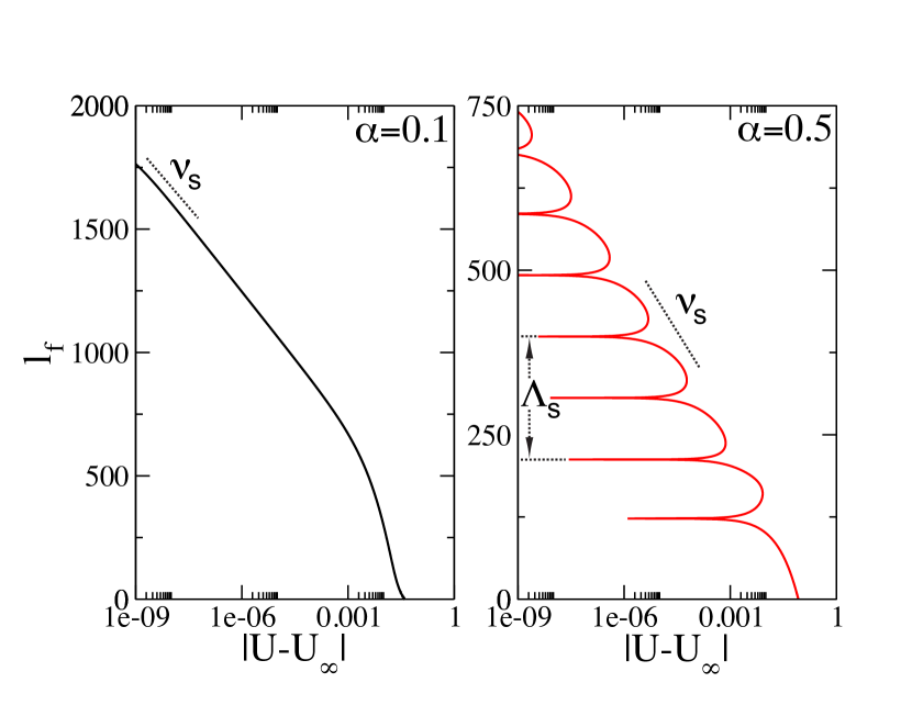
Figure 3: Comparison of bifurcation diagrams for two inclination angles as stated in the panels in th ecase without temperature gradient ($\Omega=0$). Top: Left panel: Asymptotic monotonic increase of the foot length $\l_{f}$ towards the vertical asymptote at $U=U_{\infty}$ as a function of the plate velocity $U$ for $\alpha=0.1$, which is below $\alpha_{c}$. Right panel: Snaking behaviour of the foot length $\l_{f}$ where the bifurcation curve oscillates around a vertical asymptote at $U=U_{\infty}$ with decaying amplitude of oscillations as a function of the plate velocity $U$ for $\alpha=0.5$, which is above $\alpha_{c}$. Note the appearance of pairs of saddle nodes (the first being at $U_{b}$) where the system successively switches branches and “snakes” around $U_{\infty}$. Bottom: In order to illustrate the different behaviour for angles below and above $\alpha_{c}$, we show the foot-length measure $\l_{f}$ versus $|U-U_{\infty}|$ in a semi-log plot. Left panel: The semi-log plot shows an asymptotic monotonic growth in $U$. Right panel: An exponential – oscillating periodic decay is clearly shown. A periodic structure with a snaking wavelength $\Lambda_{s}$ and an exponential decay rate $\nu_{s}$ appears after $U_{b}$ (bifurcation: appearance of the first saddle node).

4 Numerical results

In this section, we present numerical solutions of eq. (8). We solve the equation on the domain $[-L_{1},\,L_{2}]$. At $x=-L_{1}$, we impose the boundary conditions $h^{\prime}(-L_{1})=0$ and $h^{\prime\prime}(-L_{1})=0$. At $x=L_{2}$, we impose the boundary condition obtained by truncating the asymptotic expansion (45) for $\Omega\neq 0$ or (46) for $\Omega=0$ and evaluating it at $x=L_{2}$. We additionally impose a condition for the derivative of $h$ at $L_{2}$ obtained by differentiating the asymptotic expansion for $h$ and evaluating it at $x=L_{2}$. To solve this boundary-value problem numerically, we use the continuation and bifurcation software AUTO-07p (see refs. DKK91 ; DKK91b ). A description of the application of numerical continuation techniques to thin film problems can be found in sect. 4b of the review in ref. Dijk13 , in sect. 2.10 of ref. Thie07 , and in refs. TBBB03 ; BeTh10 ; TBT13 . We perform our numerical calculations on a domain with $L_{1}=9800$ and $L_{2}=200$ and choose $G=0.001$.

In fig. 2, we compare the numerical solutions with the derived asymptotic expressions for $h$ as $x\rightarrow\infty$, when the inclination angle is $\alpha=0.5$. In the left panel, $\Omega=0$ and $U=0.084$. The solid line shows a numerically computed profile, in which we can identify three regions, namely, a thin precursor film, a foot, and a bath region. We also show the truncated asymptotic expansion (46) with one, two, three and four terms included, as is indicated in the legend. In the right panel, $\Omega=0.001$ and $U=0.076$. The solid line shows a numerically computed profile the remaining lines correspond to the truncated asymptotic expansion (45) with one, two, three, four and five terms included, as is indicated in the legend. In both cases, we can observe that the numerically computed profiles agree with the derived asymptotic expansions and including more terms gives better agreement.

In fig. 3, we present bifurcation diagrams showing the dependence of a certain solution measure quantifying the foot length on the velocity of the plate for $\Omega=0$. More precisely, the measure is defined by $\l_{f}=(V-V_{0})/(h_{f}-h_{p})$, where $V=\int_{-L_{1}}^{L_{2}}(h(x)-h_{p})\mathrm{d}x$, $h_{f}$ is the characteristic foot height, $h_{p}$ is the precursor film height for the corresponding velocity, and $V_{0}$ is equal to $V$ computed at $U=0$.

We observe that there is a critical inclination angle, $\alpha_{c}\approx 0.1025$, such that for $\alpha<\alpha_{c}$, the bifurcation curve increases monotonically towards a vertical asymptote at some value of the velocity, which we denote by $U_{\infty}$. This can be observed in the left panels of fig. 3 when $\alpha=0.1$. When $\alpha>\alpha_{c}$, we observe a snaking behaviour where the bifurcation curve oscillates around a vertical asymptote at $U=U_{\infty}$ with decaying amplitude of oscillations. This can be observed in the right panels of fig. 3 when $\alpha=0.5$. We note that in this case there is an infinite but countable number of saddle-nodes at which the slope of the bifurcation curve is vertical.

Note that $U_{\infty}$ is different for each inclination angle. The character of the steady solutions is discussed below at fig. 6.

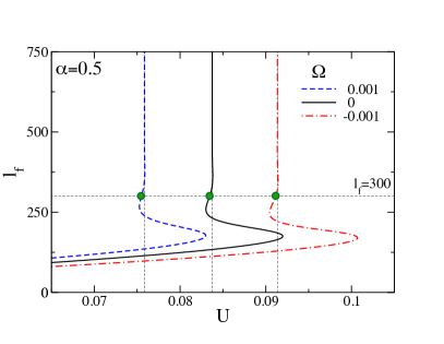
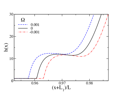
Figure 4: Left panel compares bifurcation diagrams for different temperature gradients $\Omega$ as shown in the legend for an inclination angle $\alpha=0.5$. The green filled circles indicate the points at which $\l_{f}=300$ and the corresponding film profiles are shown in the right panel. Note that the snaking behaviour is present. The temperature gradient $\Omega$ shifts the vertical asymptote at $U_{\infty}$ and changes the characteristic foot height at $U_{\infty}$.

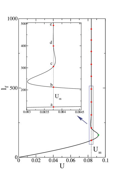
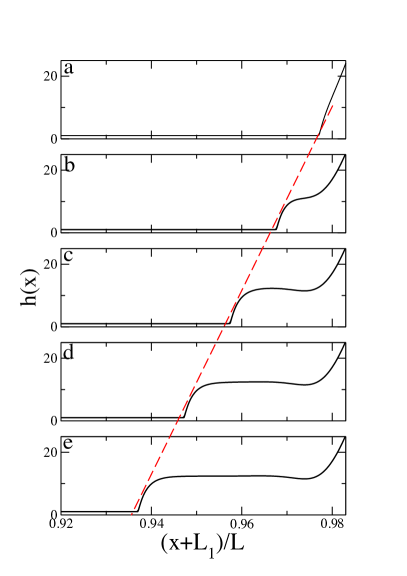
Figure 5: Film profiles at plate velocity $U_{\infty}$ for $\alpha=0.5$. Left panel: Bifurcation diagram. The red filled circles correspond to film solutions at plate velocity $U_{\infty}$. The inset shows a blow-up of the region with the first five solutions. Note the appearance of a characteristic snaking behaviour around $U_{\infty}$. The letters in the inset correspond to the film profiles depicted in the right panel. Note the appearance of undulations on top the foot-like part of the solution as the foot becomes longer. The numerical domain size used is $L=10000$, $L_{1}=9800$. Note that the first profile (a) corresponds to a meniscus solution. It is located on the lowest branch before the bifurcation curve folds back at $U_{b}$ (the green square). The red dashed line indicates a linear increase in foot length.

We note that in the case with an additional temperature gradient ($\Omega\neq 0$) we observe qualitatively similar bifurcation diagrams. If an inclination angle is below a critical value (which now depends on $\Omega$), then the bifurcation diagrams are monotonic. Otherwise, the bifurcation diagrams show snaking behaviour, as for the case of zero temperature gradient. An example of snaking bifurcation curves for $\alpha=0.5$ and $\Omega=-0.001,\,0$ and $0.001$ is given in fig. 4, and the corresponding bifurcation curves are shown by dashed, solid and dot-dashed lines. We can observe that as the temperature-gradient parameter $\Omega$ is increased/decreased, the vertical asymptote is shifted to the left/right. We can also conclude that if the temperature gradient pulls the liquid downwards, steady-state solutions of this bifurcation branch exist for larger values of $U$. Otherwise, if the temperature gradient pulls the liquid upwards, steady-state solutions of this bifurcation branch exist for smaller values of $U$. The right panel of fig. 4 shows three profiles for $l_{f}=300$ by dashed, solid and dot-dashed lines for $\Omega=0.001,\,0$ and $-0.001$, respectively. We observe that the foot height decreases as $\Omega$ decreases.

In order to illustrate the different behaviour for angles below and above $\alpha_{c}$, we also show the foot length measure, $\l_{f}$, versus $|U-U_{\infty}|$ in a semi-log plot, see the lower left and right panels of fig. 3 for $\alpha=0.1$ and $\alpha=0.5$, respectively. For $\alpha=0.1$, it can be clearly seen that the bifurcation curve approaches the vertical asymptote exponentially with a rate which we denote by $\nu_{s}$. For $\alpha=0.5$, we can see that the approach of the vertical asymptote is exponential with the snaking wavelength tending to a constant value, which we denote by $\Lambda_{s}$.

Figure 5 shows the identified snaking behaviour for $\alpha=0.5$ in more detail. In the left panel, we see the bifurcation diagram where the red filled circles correspond to solutions at $U_{\infty}$. In the chosen solution measure, the solutions appear equidistantly distributed. In the inset, the first five solutions are indicated and labeled by (a)-(e) and the corresponding film profiles are shown in the right panel. The dashed line in the right panel confirms the linear growth of the foot length.

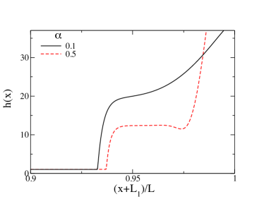
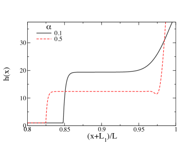
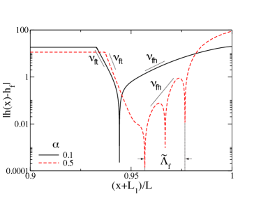
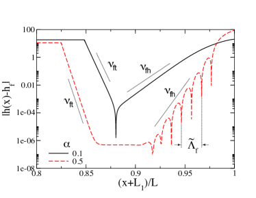
Figure 6: Film profiles below and above $\alpha_{c}$ given as solid and dashed lines, respectively. Left panel: Shown are film profiles for $\alpha=0.1$ close to $U_{\infty}$ and for $\alpha=0.5$ at $U_{\infty}$. Right panel: In order to show the appearance of undulations on top of the foot above $\alpha_{c}$, we represent in bottom panels $|h(x)-h_{f}|$ versus $(x+L_{1})/L$ in a semi-log plot, where $L_{1}=9800$, $L=10000$ is the numerical domain size and $h_{f}$ is the characteristic foot height calculated for each inclination angle $\alpha$ by solving eq. (8) for $h^{\prime}=0$, $h^{\prime\prime}=0$ and $h^{\prime\prime\prime}=0$ (using the numerically obtained value of the flux $C_{0}$). Observe the exponential approach with rate $\nu_{\mathrm{fh}}$ of the foot height from the bath side, and as well the exponential departure with rate $\nu_{\mathrm{ft}}$ from the foot height towards the precursor film (see main text for details). Note that the measured foot wavelength is $\Lambda_{f}=\widetilde{\Lambda}_{f}L$.

The differences in film profiles for angles below and above $\alpha_{c}$ can be seen in fig. 6 that shows solutions for velocities close to $U_{\infty}$ for $\alpha=0.1$ and at $U_{\infty}$ for $0.5$ by solid and dashed lines, respectively. In the left and the right panels, we compare short-foot and long-foot solutions, respectively, with similar foot lengths. To emphasise the differences, we represent the profiles in a semi-log plot $|h(x)-h_{f}|$ versus $(x+L_{1})/L$ in the bottom panels. For $\alpha=0.1$ we see no undulations – only exponential decays at a rate denoted by $\nu_{\mathrm{fh}}$ from the bath to the foot and at a rate denoted by $\nu_{\mathrm{ft}}$ from the foot to the precursor. However, for $\alpha=0.5$ we observe an oscillatory exponentially decaying behaviour at a rate denoted by $\nu_{\mathrm{fh}}$ with a wavelength denoted by $\Lambda_{f}$ in the region between the bath to the foot. In the region between the foot and the precursor film, we again observe an exponential decay.

Figures 3 to 5 allow us to recognise the observed behaviour as collapsed heteroclinic snaking noteSnaking : The bifurcation curve in fig. 5 is a snaking curve of heteroclinic orbits, i.e., each point on the curve represents a heteroclinic orbit connecting the fixed points for precursor film $\boldsymbol{y}_{p}$ and bath surface $\boldsymbol{y}_{b}$ of the dynamical system (9)-(11), namely, if $h_{p}$ and $h_{f}$ are the heights of the precursor film and the foot and $\alpha$ is the inclination angle, then the fixed points are $\boldsymbol{y}_{p}=(1/h_{p},\,0,\,0)$ and $\boldsymbol{y}_{b}=(0,\,\alpha,\,0)$, respectively. In the limit $U\to U_{\infty}$ the curve approaches a heteroclinc chain consisting of two heteroclinc orbits – one connecting the fixed points precursor film $\boldsymbol{y}_{p}$ and foot film $\boldsymbol{y}_{f}=(1/h_{f},\,0,\,0)$ and the other one connecting foot $\boldsymbol{y}_{f}$ and bath $\boldsymbol{y}_{b}$. Figure 5 (left) shows the first 5 heteroclinic orbits connecting $\boldsymbol{y}_{p}$ and $\boldsymbol{y}_{b}$ – all at $U=U_{\infty}$. In sect. 5 it is proved that at $U=U_{\infty}$ there exists a countable infinite number of such heteroclinic connections.

The values of $h_{p}$ and $h_{f}$ at $U=U_{\infty}$ are shown in fig. 7 as functions of $\alpha$ by dashed and solid lines, respectively. In fig. 8, we show the dependence of the eigenvalues of the Jacobians of system (9)-(11) at fixed points $\boldsymbol{y}_{p}$ and $\boldsymbol{y}_{f}$ at $U=U_{\infty}$ as functions of $\alpha$ (also cf. beginning of sect. 5). We note that for the precursor film all the eigenvalues are real, two of them are positive and one is negative independently of the angle. We denote these eigenvalues by $\lambda_{p,i}$, $i=1,\,2,\,3$. However for the foot, the behaviour of the eigenvalues changes for angles below and above a critical value and it turns out that this critical angle is the same as the critical angle at which monotonic bifurcation diagrams change to snaking, i.e., $\alpha_{c}\approx 0.1025$. We observe that for $\alpha<\alpha_{c}$ all the eigenvalues for the foot are real – two are positive and denoted by $\lambda_{f,1}$ and $\lambda_{f,2}$ so that $\lambda_{f,1}<\lambda_{f,2}$ and one is negative and is denoted by $\lambda_{f,3}$. However, for $\alpha>\alpha_{c}$ there is a negative real eigenvalue, $\lambda_{f,3}$, and a pair of complex conjugate eigenvalues with positive real parts, $\lambda_{f,1}$ and $\lambda_{f,2}$. Table 2 shows the values of eigenvalues $\lambda_{f,i}$, $i=1,\,2,\,3$, for $\alpha=0.1$ and $0.5$.

Table 2: Eigenvalues at fixed point $\boldsymbol{y}_{f}=(y_{1f},\,0,\,0)$ with $y_{1f}=1/h_{f}$ for $\alpha=0.1$ close to $U_{\infty}$ and for $\alpha=0.5$ at $U_{\infty}$. Note that all the eigenvalues are real for $\alpha=0.1$, whereas for $\alpha=0.5$ one eigenvalue is real and negative and two are complex conjugates with positive real parts. See fig. 8.

$\alpha$	$h_{f}$	$y_{1f}$	$\lambda_{f,1}$	$\lambda_{f,2}$	$\lambda_{f,3}$
0.1	19.3732	0.0516	0.0173	0.0188	-0.0361
0.5	12.3922	0.0807	0.0263	0.0263	-0.0525
			$+\mathrm{i}\>0.0346$	$-\mathrm{i}\>0.0346$

Table 3: Shown is the comparison of the exponential decays $\nu_{\mathrm{ft}}$, $\nu_{\mathrm{fh}}$ with the eigenvalue $\nu$ from the linear stability analysis for $\alpha=0.1$ close to $U_{\infty}$ and for $\alpha=0.5$ at $U_{\infty}$ for solutions with a short foot. See fig. 6.

$\alpha$	$\nu=\mathrm{Re}[\lambda_{f,3}]$	$\nu_{\mathrm{ft}}$	$\nu=\mathrm{Re}[\lambda_{f,1}]$	$\nu_{\mathrm{fh}}$
0.1	-0.0361	-0.0403	0.0173	0.0152
0.5	-0.0525	-0.0497	0.0263	0.0278

Table 4: Shown is the comparison of the exponential decays $\nu_{\mathrm{ft}}$, $\nu_{\mathrm{fh}}$ with the eigenvalue $\nu$ from the linear stability analysis for $\alpha=0.1$ close to $U_{\infty}$ and for $\alpha=0.5$ at $U_{\infty}$ for solutions with a long foot. See fig. 6.

$\alpha$	$\nu=\mathrm{Re}[\lambda_{f,3}]$	$\nu_{\mathrm{ft}}$	$\nu=\mathrm{Re}[\lambda_{f,1}]$	$\nu_{\mathrm{fh}}$
0.1	-0.0361	-0.0356	0.0173	0.0155
0.5	-0.0525	-0.0463	0.0263	0.0255

Table 5: Shown is the comparison of the wavelength of snaking $\Lambda_{s}$ from the bifurcation diagram and wavelength of the undulations of the foot $\Lambda_{f}$ from the foot-like profile with the wavelength $\Lambda$ calculated from the eigenvalues $\lambda_{f,i}$ at $U_{\infty}$ for $\alpha=0.5$. Note the locking between $\Lambda\approx\Lambda_{s}\approx\Lambda_{f}$. See fig. 3 and fig. 6.

$\alpha$	$\Lambda\!\!=\!\!2\pi/\mathrm{Im}[\lambda_{f,1}]$	$\Lambda_{f}\,$(long)	$\Lambda_{f}\,$(short)	$\Lambda_{s}$
0.5	181.6987	202.6920	198.8801	184.7657

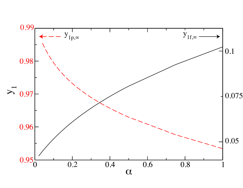
Figure 7: $y_{1}$ ($y_{1}=1/h$) at fixed points for precursor film height, $h_{p}$, ($y_{1p}=1/h_{p}$), and foot film height, $h_{f}$, ($y_{1f}=1/h_{f}$), versus inclination angle $\alpha$ at $U_{\infty}$ shown by dashed and solid lines, respectively, in a double entry plot. Note that the correct numerically obtained flux $C_{0}$ is needed at each $\alpha$ to determine the fixed points. The left side of the ordinate axis corresponds to the precursor film, the right side corresponds to the foot.

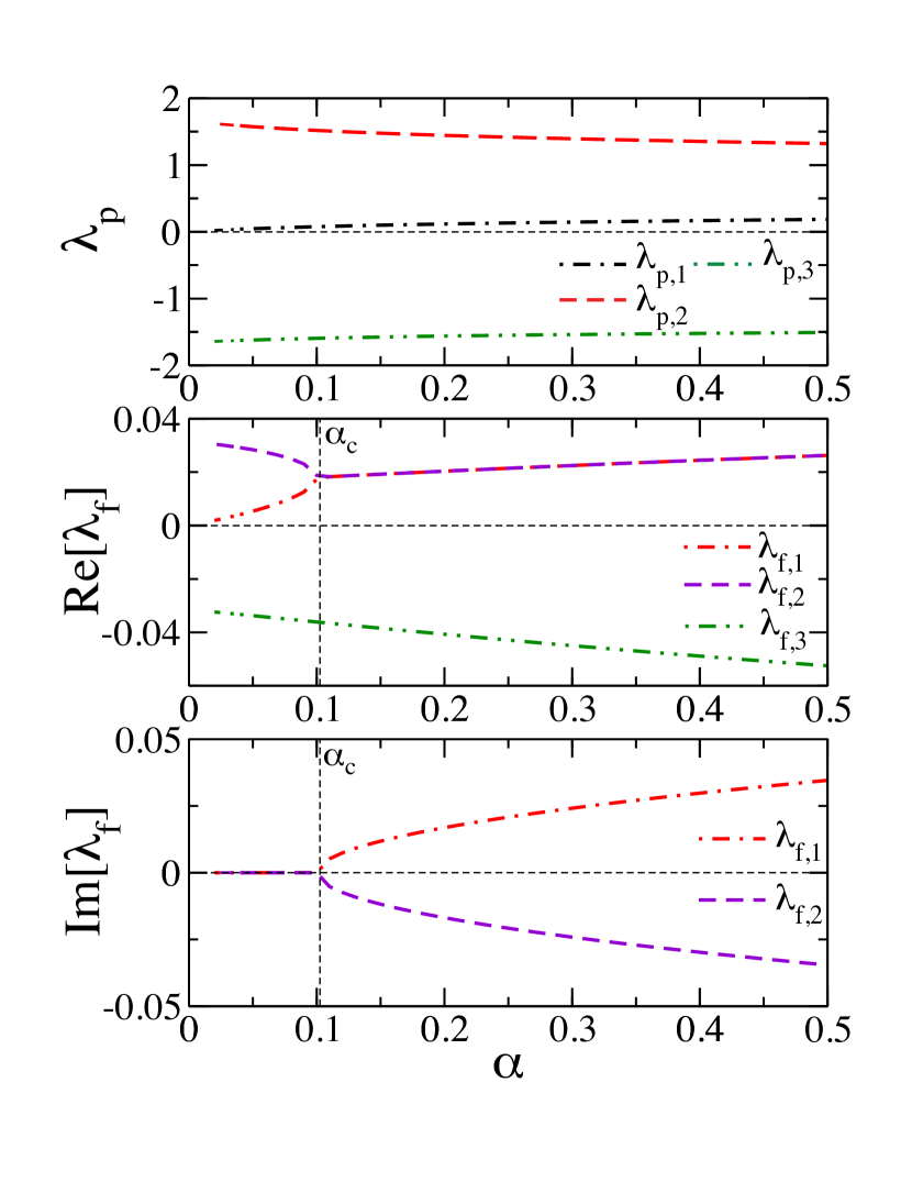
Figure 8: Eigenvalues at corresponding $U_{\infty}$ for each $\alpha$. Upper panel: Shown are the three eigenvalues $\lambda_{p}$ versus $\alpha$ for the fixed point corresponding to the precursor film. Note that all the eigenvalues are real. Middle and bottom panels: Show are the real and the imaginary parts, respectively, of the three eigenvalues $\lambda_{f}$ versus $\alpha$ for the fixed corresponding to the foot.

In tables 3 and 4, we compare $\mathrm{Re}[\lambda_{f,3}]$ with the exponential rate $\nu_{\mathrm{ft}}$ characterising the connection between the foot and the precursor film, and $\mathrm{Re}[\lambda_{f,1}]$ with the exponential rate $\nu_{\mathrm{fh}}$ characterising the connection between the foot and the bath. Table 3 corresponds to a short foot, while table 4 corresponds to a long foot. For $\alpha=0.5$ the plate velocity is equal to $U_{\infty}$, while for $\alpha=0.1$ we choose a foot of approximately the same lengths as for $\alpha=0.5$ and we note that for $\alpha=0.1$ the bifurcation curves do not reach $U_{\infty}$, but for the chosen foot the velocities coincide with $U_{\infty}$ up to at least seven significant digits. The results show that there is good agreement between $\mathrm{Re}[\lambda_{f,3}]$ and $\nu_{\mathrm{ft}}$ and between $\mathrm{Re}[\lambda_{f,1}]$ and $\nu_{\mathrm{fh}}$ for both values of $\alpha$ and for both foot lengths, with a maximal error below $12\%$.

Table 6: Shown is the comparison of the exponential decay constant $1/\nu_{S}$ from the bifurcation diagrams with the eigenvalues $\lambda_{f,i}$ calculated from the linear stability analysis for $\alpha=0.1$ and $\alpha=0.5$. See fig. 3.

$\alpha$	$\mathrm{Re}[\lambda_{f,1}]$	$1/\nu_{s}$
0.1	0.0173	0.0151
0.5	0.0263	0.0284

In table 5 we compare $\Lambda=2\pi/\mathrm{Im}[\lambda_{f,1}]$ with the wavelength of the oscillations on the foot, $\Lambda_{f}$, for a long and a short foot, and with the wavelength of oscillations in snaking bifurcation diagrams, $\Lambda_{s}$, when $\alpha=0.5$. The results show that there is good agreement between $\Lambda$ and $\Lambda_{s}$ – the error is below $2\%$, and between $\Lambda$ and $\Lambda_{f}$ for both foot lengths – the error is below $12\%$ noteMeasure .

In table 6, we compare $\mathrm{Re}[\lambda_{f,1}]$ with the exponential rate $1/\nu_{s}$, where $\nu_{s}$ is characterises the rate at which the bifurcation diagrams approach the vertical asymptotes. We again observe good agreement for both values of $\alpha$, with an error up to $13\%$.

The close agreement between the eigenvalues corresponding to the foot and the quantities obtained from the bifurcation diagrams and the foot profiles is explained in the next section.

5 Collapsed heteroclinic snaking

In what follows, our aim is to explain the snaking behaviour observed in our numerical results, see the left panels of fig. 3 and fig. 5. We perform our analysis in the way similar to the Shilnikov-type method for studying subsidiary homoclinic orbits near the primary one explained in, e.g., ref. GlSp1984jsp . For simplicity, we consider the case of zero temperature gradient, i.e., we set $\Omega=0$. First, let us consider fixed points of system (9)-(11) with $y_{1}\neq 0$. For such fixed points, $y_{2}=y_{3}=0$ and $y_{1}$ satisfies the equation

$$f(y_{1})\equiv y_{1}^{3}-\frac{U}{C_{0}}y_{1}^{2}+\frac{G\alpha}{C_{0}}=0.$$ (50)

It can be easily checked that this cubic polynomial has a local maximum at $y_{1}^{a}=0$ and a local minimum at a positive point $y_{1}^{b}$. Moreover, $f(y_{1}^{a})>0$ implying that there is always a fixed point with a negative value of the $y_{1}$-coordinate. We disregard this point, since physically it would correspond to negative film thickness. Also, assuming that $G\alpha<(4/27)(U^{3}/C_{0}^{2})$, we obtain $f(y_{1}^{b})<0$, which implies that there are two positive roots $a_{1}$ and $a_{2}$ of the cubic polynomial satisfying $a_{1}<a_{2}$. This implies that there are two more fixed points, $\boldsymbol{y}_{f}=(a_{1},\,0,\,0)$ and $\boldsymbol{y}_{p}=(a_{2},\,0,\,0)$. The point $\boldsymbol{y}_{f}$ corresponds to the foot and the point $\boldsymbol{y}_{p}$ corresponds to the precursor film.

To analyse stability of these fixed points, we compute the Jacobian at these points,

$$\!J_{\boldsymbol{y}_{f,p}}=\!\left(\begin{array}[]{ccc}0&-a_{1,2}^{2}&0\\ 0&0&1\\ 2Ua_{1,2}-3C_{0}a_{1,2}^{2}&\,\,6a_{1,2}^{7}-3a_{1,2}^{4}+G&0\end{array}\right).\!\!$$ (51)

A simple calculation shows that for both, $\boldsymbol{y}_{f}$ and $\boldsymbol{y}_{p}$, all the eigenvalues have non-zero real parts implying that these points are hyperbolic. Moreover, both points have two-dimensional unstable manifolds and one-dimensional stable manifolds. Our numerical simulations presented in the previous section show that for the values of the inclination angle $\alpha$ that we have considered, there exists a value of the plate speed, $U_{\infty}$, such that in the vicinity of this value there exist steady solutions for which the foot length can be arbitrarily long, see fig. 3. (In fact, we found that this is true if $\alpha$ is smaller than a certain transition value $\alpha_{T}\approx 2.42$. For larger values of $\alpha$, the solution branches originating from $U=0$ are not anymore characterised by such limiting velocities. In the present manuscript, we do not consider such solutions and assume therefore that $\alpha<\alpha_{T}$. Other types of solutions will be analysed elsewhere.) We conclude that at $U=U_{\infty}$, there exists a heteroclinic chain connecting the fixed points $\boldsymbol{y}_{p}$, $\boldsymbol{y}_{f}$ and $\boldsymbol{y}_{b}$. As was discussed in the previous section, in the top panel of fig. 8, we can observe that for point $\boldsymbol{y}_{p}$ all the eigenvalues are real at $U=U_{\infty}$ implying that this point is a saddle. The two bottom panels of fig. 8 demonstrate that there is a critical inclination angle $\alpha_{c}\approx 0.1025$ such that for $\alpha\leq\alpha_{c}$, all the eigenvalues for $\boldsymbol{y}_{f}$ are real, whereas for $\alpha>\alpha_{c}$, one eigenvalue is real and negative and there is a pair of complex conjugate eigenvalues with positive real parts. Therefore, for $\alpha\leq\alpha_{c}$, point $\boldsymbol{y}_{f}$ is a saddle, but for $\alpha>\alpha_{c}$, it is a saddle-focus. In the following Theorem, we analytically prove that if $\boldsymbol{y}_{f}$ is a saddle-focus, there exists an infinite but countable number of subsidiary heteroclinic orbits connecting $\boldsymbol{y}_{p}$ and $\boldsymbol{y}_{b}$ that lie in a sufficiently small neighbourhood of the heteroclinic chain connecting $\boldsymbol{y}_{p}$, $\boldsymbol{y}_{f}$ and $\boldsymbol{y}_{b}$. This explains the existence of an infinite but countable number of steady-state solutions having different foot lengths observed in the previous section, see the left panels of fig. 3 and fig. 5. Note that an infinite but countable number of solutions has also been observed in, e.g., ref. [16] for the case of a liquid film rising onto a resting inclined plate driven by Marangoni forces due to a temperature gradient. There, the authors identify type 1 and type 2 solutions with small and large far-field thicknesses, respectively. These correspond to our precursor and foot height, respectively. It is observed that for certain parameter values there exists an infinite but countable number of type 2 solutions. Similar to our case, this can be explained by the existence of a heteroclinic chain connecting the three fixed points. However, unlike here, in ref. [16] the chain connects the fixed point for the thick film along its unstable manifold with the fixed point for the thin film thickness that is then connected with the fixed point for the bath.

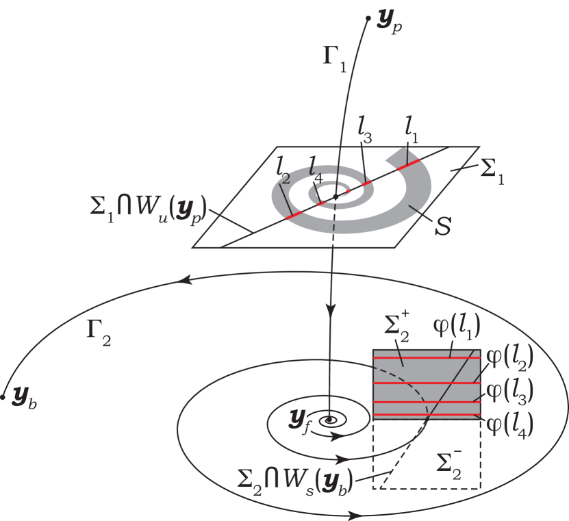
Figure 9: Schematic representation in the three-dimensional phase-space of the fixed points $\boldsymbol{y}_{p}$, $\boldsymbol{y}_{f}$ and $\boldsymbol{y}_{b}$ of system (52) when $\beta=\beta_{0}$. The fixed point $\boldsymbol{y}_{p}$ is a saddle point with two-dimensional unstable manifold, $W_{u}(\boldsymbol{y}_{p})$, and a one-dimensional stable manifold. The fixed point is $\boldsymbol{y}_{f}$ is a saddle-focus with two-dimensional unstable manifold and a one-dimensional stable manifold. The fixed point $\boldsymbol{y}_{b}$ is a non-hyperbolic point having two-dimensional stable manifold, $W_{s}(\boldsymbol{y}_{b})$. The fixed points $\boldsymbol{y}_{p}$ and $\boldsymbol{y}_{f}$ are connected by the heteroclinic orbit $\Gamma_{1}$ and the fixed points $\boldsymbol{y}_{f}$ and $\boldsymbol{y}_{b}$ are connected by the heteroclinic orbit $\Gamma_{2}$.

Theorem. Consider a three-dimensional system

$$\boldsymbol{y}^{\prime}=\boldsymbol{f}(\boldsymbol{y},\,\beta),\qquad\boldsymbol{y}\in\mathbb{R}^{3},$$ (52)

where $\beta$ denotes a parameter (that takes the role of the plate velocity $U$ above). We assume that there exist three fixed points, which we denote by $\boldsymbol{y}_{p}$, $\boldsymbol{y}_{f}$ and $\boldsymbol{y}_{b}$, when $\beta$ is sufficiently close to a number $\beta_{0}$ (i.e., a number like the plate velocity $U_{\infty}$). We additionally assume that $\boldsymbol{y}_{p}$ and $\boldsymbol{y}_{b}$ have a two-dimensional unstable manifold $W_{u}(\boldsymbol{y}_{p})$ and a two-dimensional stable manifold $W_{s}(\boldsymbol{y}_{b})$, respectively, and that $\boldsymbol{y}_{f}$ is a saddle-focus fixed point with a one-dimensional stable manifold $W_{s}(\boldsymbol{y}_{f})$ and a two-dimensional unstable manifold $W_{u}(\boldsymbol{y}_{f})$ (i.e., the eigenvalues of the Jacobian at $\boldsymbol{y}_{f}$ are $-\lambda_{1}$, $\lambda_{2}\pm\mathrm{i}\>\omega$, where $\lambda_{1}=\lambda_{1}(\beta)$, $\lambda_{2}=\lambda_{2}(\beta)$ and $\omega=\omega(\beta)$ are positive real numbers when $\beta$ is sufficiently close to $\beta_{0}$) noteManifold . Let us also assume that for $\beta=\beta_{0}$, there is a heteroclinic orbit $\Gamma_{1}\in W_{u}(\boldsymbol{y}_{p})\cap W_{s}(\boldsymbol{y}_{f})$ connecting $\boldsymbol{y}_{p}$ and $\boldsymbol{y}_{f}$ and that the manifolds $W_{u}(\boldsymbol{y}_{f})$ and $W_{s}(\boldsymbol{y}_{b})$ intersect transversely so that there is a heteroclinic orbit $\Gamma_{2}\in W_{u}(\boldsymbol{y}_{f})\cap W_{s}(\boldsymbol{y}_{b})$ connecting $\boldsymbol{y}_{f}$ and $\boldsymbol{y}_{b}$. Then for $\beta=\beta_{0}$ there is an infinite but countable number of heteroclinic orbits connecting $\boldsymbol{y}_{p}$ and $\boldsymbol{y}_{b}$ and passing near $\boldsymbol{y}_{f}$. Moreover, the difference in ‘transition times’ from $\boldsymbol{y}_{p}$ to $\boldsymbol{y}_{b}$ tends asymptotically to $\pi/\omega$ (the meaning of a ‘transition time’ from $\boldsymbol{y}_{p}$ to $\boldsymbol{y}_{b}$ will be explained below).

Proof: After a suitable change of variables, the dynamical system $\boldsymbol{y}^{\prime}=\boldsymbol{f}(\boldsymbol{y},\,\beta)$ can be written in the form

$$y_{1}^{\prime} = \lambda_{2}y_{1}-\omega y_{2}+\tilde{f}_{1}(\boldsymbol{y},\,\beta),$$ (53)

$$y_{2}^{\prime} = \omega y_{1}+\lambda_{2}y_{2}+\tilde{f}_{2}(\boldsymbol{y},\,\beta),$$ (54)

$$y_{3}^{\prime} = -\lambda_{1}y_{3}+\tilde{f}_{3}(\boldsymbol{y},\,\beta),$$ (55)

where $\tilde{f}_{i}$, $i=1,\,2,\,3$, are such that $\partial\tilde{f}_{i}/\partial y_{j}=0$, $i,\,j=1,\,2,\,3$, at $\boldsymbol{y}=\boldsymbol{y}_{f}$. After such a change of variables, the origin is a stationary point corresponding to $\boldsymbol{y}_{f}$ and sufficiently close to the origin, the terms $\tilde{f}_{1}(\boldsymbol{y},\,\beta)$, $\tilde{f}_{2}(\boldsymbol{y},\,\beta)$ and $\tilde{f}_{3}(\boldsymbol{y},\,\beta)$ are negligibly small, so that near the origin the dynamical system can be approximated by the linearised system

$$y_{1}^{\prime} = \lambda_{2}y_{1}-\omega y_{2},$$ (56)

$$y_{2}^{\prime} = \omega y_{1}+\lambda_{2}y_{2},$$ (57)

$$y_{3}^{\prime} = -\lambda_{1}y_{3}.$$ (58)

Let $\Sigma_{1}$ be a plane normal to the stable manifold of $\boldsymbol{y}_{f}$, $\Gamma_{1}$, and located at a small distance $\varepsilon_{1}$ from $\boldsymbol{y}_{f}$, i.e., locally $\Sigma_{1}$ is given by

$$\Sigma_{1}=\{(y_{1},\,y_{2},\,\varepsilon_{1}):\,y_{1},\,y_{2}\in\mathbb{R}\}.$$ (59)

Let $\Sigma_{2}$ be part of a plane transversal to the unstable manifold of $\boldsymbol{y}_{f}$, $\Gamma_{2}$, at some point near $\boldsymbol{y}_{f}$ and passing through $\boldsymbol{y}_{f}$ that is locally given by

$$\Sigma_{2}=\{(y_{1},\,0,\,y_{3}):\,|y_{1}-r^{*}|\leq\varepsilon_{2},\,|y_{3}|\leq\varepsilon_{3}\}.$$ (60)

Here $(r^{*},\,0,\,0)\in\Gamma_{1}$ is sufficiently close to the origin and $\varepsilon_{3}<\varepsilon_{1}$. We denote the upper half-plane of $\Sigma_{2}$, when $y_{3}>0$, by $\Sigma_{2}^{+}$, i.e., $\Sigma_{2}^{+}=\{\boldsymbol{y}\in\Sigma_{2}:\,y_{3}>0\}$ and let $\Sigma_{2}^{-}=\Sigma_{2}\backslash\Sigma_{2}^{+}$. We choose $\varepsilon_{2}$ to be sufficiently small so that each trajectory crosses $\Sigma_{2}$ only once. It can be shown that this condition is satisfied when $\varepsilon_{2}<\tanh(\lambda_{2}\pi/\omega)\>r^{*}$.

Using cylindrical polar coordinates $(r,\,\theta,\,z)$, such that $y_{1}=r\cos\theta$, $y_{2}=r\sin\theta$ and $y_{3}=z$, the linearised dynamical system near the origin is given by

$$r^{\prime} = \lambda_{2}r,$$ (61)

$$\theta^{\prime} = \omega,$$ (62)

$$z^{\prime} = -\lambda_{1}z.$$ (63)

The solution is given by

$$r = r_{0}\mathrm{e}^{\lambda_{2}x},$$ (64)

$$\theta = \theta_{0}+\omega x,$$ (65)

$$z = z_{0}\mathrm{e}^{-\lambda_{1}x}.$$ (66)

In the cylindrical polar coordinates, $\Sigma_{1}$ is given by $z=\varepsilon_{1}$ and $\Sigma_{2}$ is given by

$$\Sigma_{2}=\{(r,\,0,\,z):\,|r-r^{*}|\leq\varepsilon_{2},\,|z|\leq\varepsilon_{3}\}.$$ (67)

Let $\varphi_{x}$ be the flow map for the linearised dynamical system. Also, let $S$ be the set in $\Sigma_{1}$ given by

$$S=\{\boldsymbol{y}\in\Sigma_{1}:\,\exists\>x\text{ such that }\varphi_{x}(\boldsymbol{y})\in\Sigma_{2}\}.$$ (68)

Then we can define the map

$$\varphi:S\rightarrow\Sigma_{2}:\,\boldsymbol{y}\mapsto\varphi_{x}(\boldsymbol{y})\text{ for some }x>0.$$ (69)

It can easily be checked that the image of $\varphi$ is in fact $\Sigma_{2}^{+}$. Also, it can be easily seen that the set $S$ is the so-called Shilnikov snake, a set bounded by two spirals, $s_{1}$ and $s_{2}$, given by

$$r=(r^{*}\pm\varepsilon_{2})\mathrm{e}^{-\lambda_{2}x},\quad\theta=-\omega x,\quad z=\varepsilon_{1},$$ (70)

respectively, where $x\in[(1/\lambda_{1})\log(\varepsilon_{1}/\varepsilon_{3}),\,\infty)$, and the following segment of a straight line:

$$\displaystyle r\in\left[(r^{*}-\varepsilon_{2})\left(\frac{\varepsilon_{3}}{\varepsilon_{1}}\right)^{\lambda_{2}/\lambda_{1}},\,(r^{*}+\varepsilon_{2})\left(\frac{\varepsilon_{3}}{\varepsilon_{1}}\right)^{\lambda_{2}/\lambda_{1}}\right],\,\,\,$$ (71)

$$\displaystyle\theta=\frac{\omega}{\lambda_{1}}\log\left(\frac{\varepsilon_{3}}{\varepsilon_{1}}\right),\quad z=\varepsilon_{1}.$$ (72)

Let $l_{p}=\Sigma_{1}\cap W_{u}(\boldsymbol{y}_{p})$ be the intersection of the two-dimensional unstable manifold of $\boldsymbol{y}_{p}$ and the plane $\Sigma_{1}$, which is locally a straight line given for $\beta=\beta_{0}$ by the equations $\theta=\theta_{p}$ and $z=\varepsilon_{1}$, where $\theta_{p}$ is some constant. As $\theta_{p}\,\mathrm{mod}\,\pi$ determines the direction of the line, we can choose without out loss of generality,

$$\theta_{p}\in(-\pi+(\omega/\lambda_{1})\log(\varepsilon_{3}/\varepsilon_{1}),\,(\omega/\lambda_{1})\log(\varepsilon_{3}/\varepsilon_{1})].$$ (73)

Next, let $l_{n}$, $n=1,\,2,\,\ldots,$ be the intersections of the line $l_{p}$ with set $S$ such that $|l_{1}|>|l_{2}|>\cdots,$ where $|l_{n}|$ denotes the length of the segment $l_{n}$, $n=1,\,2,\,\ldots,$ see fig. 9. We can see that $l_{n}$ is given by

$$r\in[(r^{*}-\varepsilon_{2})\exp(-\lambda_{2}(\pi(n-1)-\theta_{p})/\omega),\,$$

$$\qquad(r^{*}+\varepsilon_{2})\exp(-\lambda_{2}(\pi(n-1)-\theta_{p})/\omega)],$$ (74)

$$\theta=\theta_{p}-\pi(n-1)=\theta_{p}\,\mathrm{mod}\,\pi,\quad z=\varepsilon_{1}.$$ (75)

Then, we find that $\varphi(l_{n})$ is a segment of a line in $\Sigma_{2}$ given by

$$r\in[(r^{*}-\varepsilon_{2}),\,(r^{*}+\varepsilon_{2})],$$ (76)

$$\theta=0,$$ (77)

$$z=\varepsilon_{1}\exp(-\lambda_{1}(\pi(n-1)-\theta_{p})/\omega).$$ (78)

Let $l_{b}=\Sigma_{2}\cap W_{s}(\boldsymbol{y}_{b})$ be the intersection of the two-dimensional stable manifold of $\boldsymbol{y}_{b}$ and the plane $\Sigma_{2}$. Locally it is a segment of a straight line, and since manifolds $W_{u}(\boldsymbol{y}_{f})$ and $W_{u}(\boldsymbol{y}_{b})$ intersect transversely, this segment of the line is given for $\beta=\beta_{0}$ by parametric equations

$$r=r^{*}+as,\quad\theta=0,\quad z=s,$$ (79)

where $a$ is some constant and $s$ is a parameter changing from $-\varepsilon_{3}$ to $\varepsilon_{3}$. Note that we can choose $\varepsilon_{3}$ to be smaller than $\varepsilon_{2}/|a|$ so that the line $l_{b}$ intersects all the lines $\varphi(l_{n}),$ $n=1,\,2,\,\ldots,$ and we denote such intersections points by $\boldsymbol{y}_{b,n},$ $n=1,\,2,\,\ldots.$ Let us denote the preimages of these points with respect to map $\varphi$ by $\boldsymbol{y}_{p,n},$ $n=1,\,2,\,\ldots.$ Note that $\boldsymbol{y}_{p,n}\in l_{n},$ $n=1,\,2,\,\ldots.$ Next, since for each $n=1,\,2,\,\ldots,$ point $\boldsymbol{y}_{p,n}$ belongs to the unstable manifold of $\boldsymbol{y}_{p}$, there is an orbit $\Gamma_{p,n}$ connecting $\boldsymbol{y}_{p}$ and $\boldsymbol{y}_{p,n}$. Also, by definition of point $\boldsymbol{y}_{p,n}$, it is mapped by the flow map $\varphi_{x}$ to point $\boldsymbol{y}_{b,n}$ and the ‘transition time’ from $\boldsymbol{y}_{p,n}$ to $\boldsymbol{y}_{b,n}$ is approximately equal to $x=t_{\mathrm{tr}}=(\pi(n-1)-\theta_{p})/\omega$. Note that the difference in ‘transition times’ from $\boldsymbol{y}_{p,n}$ to $\boldsymbol{y}_{b,n}$ and from $\boldsymbol{y}_{p,(n+1)}$ to $\boldsymbol{y}_{b,(n+1)}$ tends to $\pi/\omega$ as $n$ increases. We denote the orbit connecting $\boldsymbol{y}_{p,n}$ with $\boldsymbol{y}_{b,n}$ by $\Gamma_{f,n}$. Finally, since $\boldsymbol{y}_{b,n}$ for each $n=1,\,2,\,\ldots,$ point $\boldsymbol{y}_{p,n}$ belongs to the stable manifold of $\boldsymbol{y}_{b}$, there is an orbit $\Gamma_{b,n}$ connecting $\boldsymbol{y}_{b,n}$ and $\boldsymbol{y}_{b}$. We conclude that there is an infinite but countable number of subsidiary heteroclinic orbits connecting points $\boldsymbol{y}_{p}$ and $\boldsymbol{y}_{b}$ that are given by $\Gamma_{s,n}=\Gamma_{p,n}\cup\Gamma_{f,n}\cup\Gamma_{b,n},$ $n=1,\,2,\,\ldots.$ Moreover, the difference in ‘transition times’ for two successive orbits $\Gamma_{s,n}$ and $\Gamma_{s,(n+1)}$ taken to get from plane $\Sigma_{1}$ to plane $\Sigma_{2}$ tends to $\pi/\omega$ as $n\rightarrow\infty.$ Q.E.D.

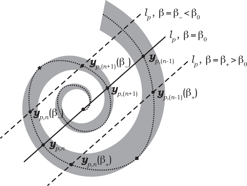
Figure 10: Schematic representation of the Shilnikov snake, $S$, in plane $\Sigma_{2}$. The solid line shows line $l_{p}$ for $\beta=\beta_{0}$, the dashed lines show lines $l_{p}$ for $\beta=\beta_{+}>\beta_{0}$ and for $\beta=\beta_{-}<\beta_{0}$. The dotted line shows the locus of the points through which heteroclinic orbits connecting $\boldsymbol{y}_{p}$ and $\boldsymbol{y}_{b}$ pass for certain values of $\beta$ near $\beta_{0}$. The black square corresponds to the value of $\beta_{+}$ at which line $\l_{p}$ is tangent to $S$ and at which points $\boldsymbol{y}_{p,(n-1)}$ and $\boldsymbol{y}_{p,n}$ vanish in a saddle-node bifurcation. The star corresponds to the value of $\beta_{-}$ at which line $\l_{p}$ is tangent to $S$ and at which points $\boldsymbol{y}_{p,n}$ and $\boldsymbol{y}_{p,(n+1)}$ vanish in a saddle-node bifurcation.

Remark. Snaking diagrams as those computed in the previous section are obtained by an unfolding of the structurally unstable heteroclinic chain connecting $\boldsymbol{y}_{p}$, $\boldsymbol{y}_{f}$ and $\boldsymbol{y}_{b}$. For $\beta$ close to $\beta_{0}$ but not necessarily equal to $\beta_{0}$, line $l_{p}=\Sigma_{1}\cap W_{u}(\boldsymbol{y}_{p})$ is locally given by

$$y_{2}=b(\beta)y_{1}+c(\beta),\quad y_{3}=\varepsilon_{1},$$ (80)

where $c(\beta_{0})=0$ and $b(\beta_{0})=\tan(\theta_{p})$ (without loss of generality, we can assume that $\theta_{p}\neq\pi/2+\pi n$ for any $n\in\mathbb{Z}$). This implies that in a small neighbourhood of point $(0,\,0,\,\varepsilon_{1})$, this line can be approximated by

$$y_{2}=(b(\beta_{0})+\Delta\beta\>b^{\prime}(\beta_{0}))y_{1}+\Delta\beta\>c^{\prime}(\beta_{0}),\quad y_{3}=\varepsilon_{1},$$ (81)

where $\Delta\beta=\beta-\beta_{0}$. Assuming that $c^{\prime}(\beta_{0})\neq 0$, we obtain that for $\beta\neq\beta_{0}$ line $l_{p}$ is shifted in plane $\Sigma_{2}$ and does not pass through point $(0,\,0,\,\varepsilon_{1})$, see fig. 10. This implies that for $\beta\neq\beta_{0}$ line $l_{p}$ intersects the Shilnikov snake, $S$, finitely many times. For sufficiently small $\Delta\beta$, we denote by $\l_{n}(\beta)$ the intersection of $l_{p}$ with $S$ that is obtained by a small shift of $l_{n}$ for $\beta=\beta_{0}$. By considerations similar to those in the proof of the previous theorem, it can be shown that in each of the line segments there is a point $\boldsymbol{y}_{p,n}(\beta)$ such that there is a heteroclinic orbit passing through this point and connecting $\boldsymbol{y}_{p}$ and $\boldsymbol{y}_{b}$. For $\beta\neq\beta_{0}$ there is only a finite number of such orbits. Figure 10 schematically shows $l_{p}$ by a solid line for $\beta=\beta_{0}$ and by dashed lines for $\beta=\beta_{+}>\beta_{0}$ and $\beta=\beta_{-}<\beta_{0}$. In addition, points $\boldsymbol{y}_{p,(n-1)}(\beta_{+})$, $\boldsymbol{y}_{p,n}(\beta_{+})$, $\boldsymbol{y}_{p,n}(\beta_{-})$ and $\boldsymbol{y}_{p,(n+1)}(\beta_{-})$ are shown. For certain value of $\beta_{+}$, points $\boldsymbol{y}_{p,(n-1)}(\beta_{+})$, $\boldsymbol{y}_{p,n}(\beta_{+})$ vanish in a saddle-node bifurcation. This point is indicated by a black square in the figure. At this point, line $l_{p}$ is tangent to the boundary of $S$. Also, for certain value of $\beta_{-}$, points $\boldsymbol{y}_{p,n}(\beta_{-})$, $\boldsymbol{y}_{p,(n+)}(\beta_{-})$ vanish in a saddle-node bifurcation. This point is indicated by a star in the figure. At this point, line $l_{p}$ is tangent to the boundary of $S$. The locus of the points through which heteroclinic orbits connecting $\boldsymbol{y}_{p}$ and $\boldsymbol{y}_{b}$ pass for certain values of $\beta$ near $\beta_{0}$ is shown by a dotted line. It can be seen that this line is a spiral, $s$, that belongs to $S$, passes through points $\boldsymbol{y}_{p,n}$ and is tangent between transitions from $\boldsymbol{y}_{p,n}$ to $\boldsymbol{y}_{p,(n+1)},$ $n=1,\,2,\ldots,$ to the boundary of $S$ given by spiral $s_{1}$. It can therefore be concluded that the bifurcation diagram showing the ‘transition time’ for heteroclinic orbits connecting $\boldsymbol{y}_{p}$ and $\boldsymbol{y}_{p}$ versus parameter $\beta$ is a snaking curve, shown schematically in fig. 11, similar to the numerically obtained cases in figs. 3, 2 and 5 for $\alpha=0.5$. There is an infinite number of such orbits in a neighbourhood of $\beta_{0}$ and there is an infinite but countable number of saddle-node bifurcations that correspond to the points at which spiral $s$ touches the boundary of the Shilnikov spiral, $S$.

We can find that the slope of the line tangent to spiral $s_{1}$ is

$$\frac{\mathrm{d}y_{2}}{\mathrm{d}y_{1}}=R\tan(\theta+\theta_{0}),$$ (82)

where $R=\sqrt{\lambda_{2}^{2}+\omega^{2}}$ and $\theta_{0}=\tan^{-1}(\omega/\lambda_{2})$. Therefore, at the points where line $l_{p}$ touches spiral $s_{1}$, we must have

$$R\tan(\theta_{n}+\theta_{0})=b(\beta_{0})+\Delta\beta_{n}b^{\prime}(\beta_{0}),$$ (83)

where $\theta_{n}$ and $\Delta\beta_{n}$ are the values of $\theta$ and $\Delta\beta$ corresponding to the $n^{\text{th}}$ saddle-node bifurcation. Thus, at these points

$$\theta_{n}=\tan^{-1}\left(\frac{b(\beta_{0})}{R}+\Delta\beta_{n}\frac{b^{\prime}(\beta_{0})}{R}\right)-\theta_{0}-\pi n,$$ (84)

for sufficiently large integer $n$. Equivalently,

$$x_{n}=-\frac{1}{\omega}\tan^{-1}\left(\frac{b(\beta_{0})}{R}+\Delta\beta_{n}\frac{b^{\prime}(\beta_{0})}{R}\right)+\frac{\theta_{0}}{\omega}+\frac{\pi}{\omega}n.$$ (85)

From this formula, we clearly see that the difference in transition times between two saddle-node bifurcations tends to $\pi/\omega$. Also, at the saddle-node bifurcations we must have

$$\!r_{n}\sin\theta_{n}\!=\!(b(\beta_{0})+\Delta\beta_{n}b^{\prime}(\beta_{0}))r_{n}\cos\theta_{n}+\Delta\beta_{n}c^{\prime}(\beta_{0}),\!\!\!\!$$ (86)

where $r_{n}=(r^{*}+\varepsilon_{2})\mathrm{e}^{-\lambda_{2}x_{n}}$, which implies

$$\Delta\beta_{n}=r_{n}\frac{\sin\theta_{n}-b(\beta_{0})\cos\theta_{n}}{c^{\prime}(\beta_{0})+b^{\prime}(\beta_{0})r_{n}}.$$ (87)

From the latter expression, we can conclude that

$$|\Delta\beta_{n}|=O(r_{n})=O(\mathrm{e}^{-\lambda_{2}x_{n}}),$$ (88)

which shows that the snaking bifurcation diagram approaches the vertical asymptote at an exponential rate, and explains the results presented in the bottom right panel of fig. 3 and in table 6.

Also, note that if $\boldsymbol{y}_{f}$ is a saddle, then the set $S$ is not a spiral but is a wedge-shaped domain. The line $l_{p}$ then passes through the vertex of this domain for $\beta=\beta_{0}$ and, generically, intersects it in the neighbourhood of the vertex only for $\beta<\beta_{0}$ but not for $\beta>\beta_{0}$ or vice versa. Then, the bifurcation diagram showing the ‘transition time’ for heteroclinic orbits connecting $\boldsymbol{y}_{p}$ and $\boldsymbol{y}_{b}$ versus parameter $\beta$ is a monotonic curve instead of a snaking curve shown in fig. 11, similarly to the case in fig. 3 for $\alpha=0.1$.

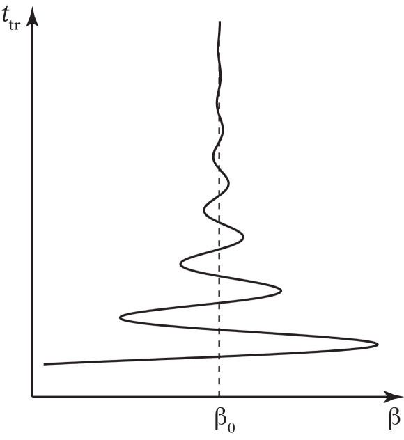
Figure 11: Bifurcation diagram for heteroclinic orbits connecting $\boldsymbol{y}_{p}$ and $\boldsymbol{y}_{b}$.

In the drawn meniscus problem the difference in transition times between two saddle-node bifurcations (that tends to $\pi/\omega$) is a measure of the wavelength of the undulations on the foot and is therefore equivalent to the measures $\Lambda_{f}$ (as extracted from the steady thickness profiles) and $\Lambda_{s}$ (as extracted from the bifurcation curve) discussed in section 4 (see, in particular, table 5 where $\Lambda$ represents $\pi/\omega$). The overall transition time corresponds to the foot length $l_{f}$. Thus one can conclude that the bifurcation diagrams presented in figs. 3 and 5 are explained by the results that have been presented in this section.

6 Conclusions

We have analysed a liquid film that is deposited from a liquid bath onto a flat moving plate that is inclined at a fixed angle to the horizontal and is removed from the bath at a constant speed. We have analysed a two-dimensional situation with a long-wave equation that is valid for small inclination angles of the plate and under the assumption that the longitudinal length scale of variations in the film thickness is much larger than the typical film thickness. The model equation used in most parts of our work includes the terms due to surface tension, the disjoining (or Derjaguin) pressure modelling wettability, the hydrostatic pressure and the lateral driving force due to gravity, the dragging by the moving plate. To further illustrate a particular finding we have also considered the situation where an additional lateral Marangoni shear stress results from a linear temperature gradient along the substrate direction. Our main goal has been to analyse selected steady-state film thickness profiles that are related to collapsed heteroclinic snaking.

First, we have used centre manifold theory to properly derive the asymptotic boundary conditions on the side of the bath. In particular, we have obtained asymptotic expansions of solutions in the bath region, when $x\rightarrow\infty$. We found that in the absence of the temperature gradient, the asymptotic expansion for the film thickness, $h$, has the form $h\sim\sum_{n=-1}^{\infty}D_{n}x^{-n}$, where without loss of generality $D_{0}$ can be chosen to be zero (fixing the value of $D_{0}$ corresponds to breaking the translational invariance of solutions and allows selecting a unique solution from the infinite family of solutions that are obtained from each other by a shift along the $x$-axis). In the presence of the temperature gradient, this asymptotic expansion is not valid, but instead consists of terms proportional to $x$, $\log x$ and $x^{-m}\log^{n}x$, where $m$ and $n$ is a positive and a non-negative integer, respectively. Note that our systematically obtained sequence differs from the one employed in ref. ME05 .

Next, we have obtained numerical solutions of the steady-state equation and have analysed the behaviour of selected solutions as the plate velocity and the temperature gradient are changed. When changing the plate velocity, we observe that the bifurcation curves exhibit collapsed heteroclinic snaking when the plate inclination angle is larger than a certain critical value, namely, they oscillate around a certain limiting velocity value, $U_{\infty}$, with an exponentially decreasing oscillation amplitude and a period that tends to some constant value. In contrast, when the plate inclination angle is smaller than the critical value, the bifurcation curve is monotonic and the velocity tends monotonically to $U_{\infty}$. The solutions along these bifurcation curves are characterised by a foot-like structure that emerges from the meniscus and is preceded by a very thin precursor film further up the plate. The length of the foot increases continuously as one follows the bifurcation curve as it approaches $U_{\infty}$. It is important to note that these solutions of diverging foot length do not converge to the Landau-Levich film solution at the same $U=U_{\infty}$. Indeed, the foot height at $U_{\infty}(\alpha)$ scales as $U^{1/2}$ while the Landau-Levich films scale as $U^{2/3}$. As expected, the results for the bifurcation curves that we here obtained with a precursor film model are similar to results obtained for such situations employing a slip model SADF07 ; ZiSnEg09 . The protruding foot structure has been observed in experiments, e.g., in refs.  SADF07 ; DFSA08 ; Snoe08 where even an unstable part of the snaking curve was tracked. However, the particular transition described here has not yet been experimentally studied. This is in part due to the fact that in an experiment with a transversal extension (fully three-dimensional system) transversal meniscus and contact line instabilities set in before the foot length can diverge. We believe that experiments in transversally confined geometries may allow one to approach the transition more closely. Experiments with driving temperature gradients exist as well but focus on other aspects of the solution structure like, for instance, various types of advancing shocks (travelling fronts) and transversal instabilities BMFC1998prl . We are not aware of studies of static foot-like structures in systems with temperature gradients.

We further note that the described monotonic and non-monotonic divergence of foot length with increasing plate velocity may be seen as a dynamic equivalent of the equilibrium emptying transition described in ref. PRJA2012prl . There, a meniscus in a tilted slit capillary develops a tongue (or foot) along the lower wall. Its length diverges at a critical slit width. In our case, the length of the foot diverges at a critical plate speed – monotonically below and oscillatory above a critical inclination angle. The former case may be seen as a continuous dynamic emptying transition with a close equilibrium equivalent. The latter may be seen as a discontinuous dynamic emptying transition that has no analogue at equilibrium. This is further analysed in ref. GTLT14 .

Finally, we have shown that in an appropriate three-dimensional phase space, the three regions of the film profile, i.e., the precursor film, the foot and the bath, correspond to three fixed points, $\boldsymbol{y}_{p}$, $\boldsymbol{y}_{f}$ and $\boldsymbol{y}_{b}$, respectively, of a suitable dynamical system. We have explained that the snaking behaviour of the bifurcation curves is caused by the existence of a heteroclinic chain that connects $\boldsymbol{y}_{p}$ with $\boldsymbol{y}_{f}$ and $\boldsymbol{y}_{f}$ with $\boldsymbol{y}_{b}$ at certain parameter values. We have proved a general result that implies that if the fixed points corresponding to the foot and to the bath have two-dimensional unstable and two-dimensional stable manifolds, respectively, and the fixed point corresponding to the foot is a saddle-focus so that the Jacobian at this point has the eigenvalues $-\lambda_{1}$, $\lambda_{2}\pm\mathrm{i}\>\omega$, where $\lambda_{1,2}$ and $\omega$ are positive real numbers, then in the neighbourhood of the heteroclinic chain there is an infinite but countable number of heteroclinic orbits connecting the fixed point for the precursor film with the fixed point for the bath. These heteroclinic orbits correspond to solutions with feet of different lengths. Moreover, these solutions can be ordered so that the difference in the foot lengths tends to $\pi/\omega$. We have also explained that in this case the bifurcation curve shows a snaking behaviour. Otherwise, if the fixed point corresponding to the foot is a saddle, the Jacobian at this point has three real non-zero eigenvalues, and the bifurcation curve is monotonic.

The presented study is by no means exhaustive. It has focused on obtaining asymptotic expansions of the solutions in the bath region using rigorous centre manifold theory and on analysing the collapsed heteroclinic snaking behaviour associated with the dragged meniscus problems. However, the system has a much richer solution structure. Beside the studied solutions one may obtain Landau-Levich films and investigate their coexistence with the discussed foot and mensicus solutions. For other solutions the bath connects directly to a precursor-type film which then connects to a thicker ‘foot-like’ film which then goes back to the precursor-type film that continues along the drawn plate. These solutions and their relation to the ones studied here will be presented elsewhere.

References

- [1] S.J. Weinstein and K.J. Ruschak. Coating flows. Annu. Rev. Fluid Mech., 36:29–53, 2004.
- [2] F.C. Morey. Thickness of a liquid film adhering to a surface slowly withdrawn from the liquid. J. Res. Nat. Bur. Stand., 25:385, 1940.
- [3] J.J. Rossum. Viscous lifting and drainage of liquids. Applied Scientific Research, Section A, 7:121–144, 1958.
- [4] R.P. Spiers, C.V. Subbaraman, and W.L. Wilkinson. Free coating of a newtonian liquid onto a vertical surface. Chem. Eng. Sci., 29(2):389 – 396, 1974.
- [5] J.H. Snoeijer, B. Andreotti, G. Delon, and M. Fermigier. Relaxation of a dewetting contact line. part 1. a full-scale hydrodynamic calculation. J. Fluid Mech., 579(-1):63–83, 2007.
- [6] G. Delon, M. Fermigier, J. H. Snoeijer, and B. Andreotti. Relaxation of a dewetting contact line. part 2. experiments. Journal of Fluid Mechanics, 604(-1):55–75, 2008.
- [7] M. Maleki, M. Reyssat, F. Restagno, D. Quéré, and C. Clanet. Journal of Colloid and Interface Science Landau – Levich menisci. Journal of Colloid and Interface Science, 354:359–363, 2011.
- [8] L. Landau and B. Levich. Dragging of a liquid by a moving plane. Acta Physicochimica U.R.S.S., 17, 1942. reprint in [51].
- [9] P. Groenveld. Low capillary number withdrawal. Chem. Eng. Sci., 25(8):1259 – 1266, 1970.
- [10] P. Groenveld. Withdrawal of power law fluid films. Chem. Eng. Sci., 25(10):1579 – 1585, 1970.
- [11] S.D.R. Wilson. The drag-out problem in film coating theory. J. Eng. Math., 16:209–221, 1981.
- [12] J. Ziegler, J.H. Snoeijer, and J. Eggers. Film transitions of receding contact lines. Eur. Phys. J. Special Topics, 166:177–180, 2009.
- [13] E.S. Benilov, S.J. Chapman, J.B. McLeod, J.R. Ockendon, and V.S. Zubkov. On liquid films on an inclined plate. J. Fluid Mech., FirstView:1–17, 2010.
- [14] B. Jin, A. Acrivos, and A. Münch. The drag-out problem in film coating. Physics of Fluids, 17(10):103603, 2005.
- [15] J.H. Snoeijer, J. Ziegler, B. Andreotti, M. Fermigier, and J. Eggers. Thick films of viscous fluid coating a plate withdrawn from a liquid reservoir. Phys. Rev. Lett., 100:244502, Jun 2008.
- [16] A. Münch and P.L. Evans. Marangoni-driven liquid films rising out of a meniscus onto a nearly-horizontal substrate. Phys. D (Amsterdam, Neth.), 209(1-4):164 – 177, 2005. Non-linear Dynamics of Thin Films and Fluid Interfaces.
- [17] H. Riegler and K. Spratte. Structural-changes in lipid monolayers during the Langmuir-Blodgett transfer due to substrate monolayer interactions. Thin Solid Films, 210:9–12, 1992.
- [18] M.H. Köpf, S.V. Gurevich, R. Friedrich, and L.F. Chi. Pattern formation in monolayer transfer systems with substrate-mediated condensation. Langmuir, 26:10444–10447, 2010.
- [19] M.H. Köpf, S.V. Gurevich, R. Friedrich, and U. Thiele. Substrate-mediated pattern formation in monolayer transfer: a reduced model. New J. Phys., 14:023016, 2012.
- [20] U. Thiele. Patterned deposition at moving contact line. Advances in Colloid and Interface Science, 2013. (online at http://dx.doi.org/10.1016/j.cis.2013.11.002).
- [21] L.P. Shilnikov. A case of the existence of a countable number of periodic motions. Sov. Math. Dokl., 6:163–166, 1965.
- [22] P Glendinning and C Sparrow. Local and global behavior near homoclinic orbits. J. Stat. Phys., 35:645–696, 1984.
- [23] J. Knobloch and T. Wagenknecht. Homoclinic snaking near a heteroclinic cycle in reversible systems. Phys. D (Amsterdam, Neth.), 206(1–2):82 Р93, 2005.
- [24] Y. P. Ma, J. Burke, and E. Knobloch. Defect-mediated snaking: A new growth mechanism for localized structures. Physica D, 239:1867–1883, 2010.
- [25] We introduce the term “collapsed heteroclinic snaking” to indicate that the corresponding bifurcation diagram consists of a snaking curve of heteroclinic orbits that is collapsed (exponentially decreasing snaking amplitude) in the sense used in Ref. [24] for homoclinic orbits close to a heteroclinic chain that connects two fixed points in a reversible system.
- [26] L.P. Shilnikov. The existence of a denumerable set of periodic motions in four-dimensional space in an extended neighborhood of a saddle-focus. Sov. Math. Dokl., 8(1):54–58, 1967.
- [27] J. Knobloch and T. Wagenknecht. Snaking of multiple homoclinic orbits in reversible systems. SIAM Journal on Applied Dynamical Systems, 7(4):1397–1420, 2008.
- [28] M. Chen. Solitary-wave and multi-pulsed traveling-wave solutions of boussinesq systems. Applicable Analysis, 75(1-2):213–240, 2000.
- [29] G.W. Hunt, M.A. Peletier, A.R. Champneys, P.D. Woods, M. Ahmer Wadee, C.J. Budd, and G.J. Lord. Cellular buckling in long structures. Nonlinear Dyn., 21(1):3–29, 2000.
- [30] A. Oron, S.H. Davis, and S.G. Bankoff. Long-scale evolution of thin liquid films. Rev. Mod. Phys., 69:931–980, Jul 1997.
- [31] U. Thiele. Structure formation in thin liquid films. In S. Kalliadasis and U. Thiele, editors, Thin Films of Soft Matter, pages 25–93, Wien, 2007. Springer.
- [32] P.-G. de Gennes. Wetting: Statics and dynamics. Rev. Mod. Phys., 57:827–863, 1985.
- [33] V.M. Starov and M.G. Velarde. Surface forces and wetting phenomena. J. Phys.-Condes. Matter, 21:464121, 2009.
- [34] U. Thiele. Thin film evolution equations from (evaporating) dewetting liquid layers to epitaxial growth. J. Phys.-Cond. Mat., 22:084019, 2010.
- [35] A.M. Cazabat, F. Heslot, S.M. Troian, and P. Carles. Fingering instability of thin spreading films driven by temperature gradients. Nature, 346(6287):824–826, August 1990.
- [36] B. Scheid, E.A. van Nierop, and H.A. Stone. Thermocapillary-assisted pulling of thin films: Application to molten metals. Appl. Phys. Lett., 97(17):171906, 2010.
- [37] B. Scheid, E.A. van Nierop, and H.A. Stone. Thermocapillary-assisted pulling of contact-free liquid films. Phys. Fluids, 24(3):032107, 2012.
- [38] J. Carr. Applications of Centre Manifold Theory. Applied Mathematical Sciences, Vol. 35. Springer-Verlag, Berlin / New York, 1981.
- [39] I.U.A. Kuznetsov. Elements of Applied Bifurcation Theory. Number vol. 112 in Applied Mathematical Sciences. Springer, New York, 1998.
- [40] E. Doedel, H.B. Keller, and J.P. Kernevez. Numerical analysis and control of bifurcation problems (I) Bifurcation in finite dimensions. Int. J. Bifurcation Chaos Appl. Sci. Eng., 1:493–520, 1991.
- [41] E. Doedel, H.B. Keller, and J.P. Kernevez. Numerical analysis and control of bifurcation problems (II) Bifurcation in infinite dimensions. Int. J. Bifurcation Chaos Appl. Sci. Eng., 1:745–72, 1991.
- [42] A. Dijkstra, F.W. Wubs, A.K. Cliffe, E. Doedel, I.F. Dragomirescu, B. Eckhart, A.Y. Gelfgat, A. Hazel, V. Lucarini, A.G. Salinger, E.T. Phipps, J. Sanchez-Umbria, H. Schuttelaars, L.S. Tuckerman, and U. Thiele. Numerical bifurcation methods and their application to fluid dynamics: Analysis beyond simulation. Commun. Comput. Phys., 2013. (at press).
- [43] U. Thiele, L. Brusch, M. Bestehorn, and M. Bär. Modelling thin-film dewetting on structured substrates and templates: Bifurcation analysis and numerical simulations. Eur. Phys. J. E, 11:255–271, 2003.
- [44] P. Beltrame and U. Thiele. Time integration and steady-state continuation method for lubrication equations. SIAM J. Appl. Dyn. Syst., 9:484–518, 2010.
- [45] D. Tseluiko, J. Baxter, and U. Thiele. A homotopy continuation approach for analysing finite-time singularities in thin liquid films. IMA J. Appl. Math., 2013. (online).
-
[46]
The wavelength is measured using the data that
are presented in fig. 6. The distances between divergencies at
, i.e., at the positions where
correspond to a semi-period of the foot wavelength . The value of
is determined as the average of all available
. Note that we can observe only up to five semi-periods due to
the exponentially decreasing amplitude of the modulation and the restricted
number of digits of the profile data obtained from auto07p. As a result, the
undulations are not detectable when their amplitude decreases below . The effect is clearly seen in the lower left panel of
fig. 6, where for we observe a plateau between the
visible undulations and the exponential decay with rate towards
the precursor film. Further, there is a limited accuracy due to the number of
discretisation points in space.
The measurement of is more exact as it makes use of the data employed in the graph (figs. 3 and 6). In contrast to the thickness profile data, these bifurcation curve data are of a high precision allowing us to see about 10 semi-periods. is measured only taking values of the semi-periods that have already converged to 3 significant digits, i.e., at (cf. fig. 3). Several such values corresponding to the length of a semi-period of the snaking wavelength are then averaged to obtain . This ensures that nonlinear effects do not enter the picture (that are likely to be present in the measurement). - [47] Here, the unstable manifold of refers to the set of points such that as , where is the solution (or evolution) operator for the given dynamical system, and the stable manifold of refers to the set of points such that as . These definitions are consistent with those given, e.g., in ref. [52].
- [48] A. L. Bertozzi, A. Münch, X. Fanton, and A. M. Cazabat. Contact line stability and ”undercompressive shocks” in driven thin film flow. Phys. Rev. Lett., 81:5169–5173, 1998.
- [49] A. O. Parry, C. Rascon, E. A. G. Jamie, and D. G. A. L. Aarts. Capillary emptying and short-range wetting. Phys. Rev. Lett., 108:246101, 2012.
- [50] M. Galvagno, D. Tseluiko, H. Lopez, and U. Thiele. Continuous and discontinuous dynamic unbinding transitions in drawn film flow. 2013. (submitted).
- [51] P. Pelce, editor. Dynamics of curved fronts. Academic Press, London, 1. edition, 1988.
- [52] R.C. Robinson. An introduction to dynamical systems: continuous and discrete. Pearson Prentice Hall, Upper Saddle River (NJ), 2004.