Introducing Pietarinen expansion method into
single-channel pole extraction problem

Abstract

We present a new approach to quantifying pole parameters of single-channel processes based on a Laurent expansion of partial-wave T-matrices in the vicinity of the real axis. Instead of using the conventional power-series description of the non-singular part of the Laurent expansion, we represent this part by a convergent series of Pietarinen functions. As the analytic structure of the non-singular part is usually very well known (physical cuts with branch points at inelastic thresholds, and unphysical cuts in the negative energy plane), we find that one Pietarinen series per cut represents the analytic structure fairly reliably. The number of terms in each Pietarinen series is determined by the quality of the fit. The method is tested in two ways: on a toy model constructed from two known poles, various background terms, and two physical cuts, and on several sets of realistic $\pi$N elastic energy-dependent partial-wave amplitudes (GWU/SAID - GWU ; GWU1 , and Dubna-Mainz-Taipei - DMT0 ; DMT ). We show that the method is robust and confident using up to three Pietarinen series, and is particularly convenient in fits to amplitudes, such as single-energy solutions, coming more directly from experiment; cases where the analytic structure of the regular part is a-priori unknown.

I Introduction

Revisions to the Review of Particle Properties PDG and contributions to the recent Camogli workshop Camogli2012 , among others, have emphasised the fact that poles, and not Breit-Wigner parameters, determine and quantify resonance properties, and that they should be used as a link between scattering theory and QCD. However, at the same time, the question of finding an adequate procedure to extract pole parameters from single-channel T-matrices remains open. Experimentalists are quite familiar with fits to data using Breit-Wigner functions (either with constant parameters and very general backgrounds, or with energy dependent masses and widths), but are less experienced when complex energy poles are to be used. Simple procedures for pole extraction exist, but are not reliable in all cases. At present, poles are usually extracted from theoretical single or multi-channel models, fitted to the data, using an array of standard pole extraction methods: analytic continuation of the model functions into the complex energy plane Doering ; EBAC ; CMB ; Zagreb ; Bonn , speed plot Hoehler93 , time delay Kelkar , N/D method ChewMandelstam , regularization procedure Ceci2008 , etc. However, this typically requires solving an involved single/coupled-channel model and analyzing the obtained analytic solution, which implicitly contains both parts: singular and background. Hence, the analytic form of the full solution varies from model to model; the pole-background separation method is not unique, and requires an intimate knowledge of the underlying model. The intention of this paper is to offer a simple, robust and confident method to obtain scattering-matrix poles, while avoiding the use of any particular assumptions concerning the form of background terms. We base our analysis on a Laurent expansion of partial wave T-matrices, which uniquely separates singular from finite terms, and treat singular and finite terms separately. Our main assumption is that all scattering matrix poles are of the first order.

II Formalism

II.1 Laurent expansion

We start with a fact that each single-channel scattering matrix is a fully analytic function in the complex energy plane with a well defined number of poles and cuts, and all knowledge from complex analysis may be applied directly to it. Consider first the Laurent expansion of a complex analytic function, $f(z)$. At the most basic level, we have the statement:

Suppose that f is holomorphic in the annulus {$z\in\mathbb{C}$, $R_{1}<|z-z_{0}|<R_{2}$}, where $0\leq R_{1}<R_{2}<\infty$. Then we can write f as a Laurent series: for $R_{1}<|z-z_{0}|<R_{2}$ we have

$$f(z) = \sum_{n=0}^{\infty}a_{n}(z-z_{0})^{n}+\sum_{n=1}^{\infty}a_{-n}(z-z_{0})^{-n}$$ (1)

This theorem basically says that each complex function defined in the full complex energy plane can locally be represented by a power series. Observe that this is not an identity in the full complex energy plane, the globally unknown, complicated function $f(z)$ can locally (in the vicinity of the singularity) be represented by a simpler function consisting of energy independent pole contribution(s) and a usually limited number of power series terms.

Applied to a single channel scattering matrix in the vicinity of one simple pole at $\omega=\omega_{0}$ in the complex energy plane $\omega$, adjusted to the sign conventions of PDG PDG , we have:

$$T(\omega) = \frac{a_{-1}}{\omega_{0}-\omega}+\sum_{n=0}^{\infty}a_{n}(\omega_{0}-\omega)^{n};$$ (2)

$$\,\,\,\,a_{n},\,\omega,\,\omega_{0}\in\mathbb{C}.$$

This expression is simply the generalization of a Taylor’s expansion of an analytic function about any regular point to the expansion of singular function around a singular point, $\omega_{0}$, and as such is a unique representation of the function over a part of the complex energy plane defined by its radius of convergence.

However, the functions we consider may (and do) contain more than one pole for $\omega\neq\omega_{0}$. If we iterate this procedure using the Mittag-Leffler theorem Mittag-Leffler , which says that a meromorphic function can be expressed in terms of its poles and associated residues combined with an additional entire function, we can, without loss of generality, write down the generalized Laurent expansion for the function with $k$ poles:

$$T(\omega) = \sum_{i=1}^{k}\frac{a_{-1}^{(i)}}{\omega_{i}-\omega}+B^{L}(\omega);$$ (3)

$$\,\,\,\,a_{-1}^{(i)},\omega_{i},\omega\in\mathbb{C},$$

where $k$ is number of poles. $a_{-1}^{(i)}$ and $\omega_{i}$ are residua and pole positions for i-th pole respectively, and $B^{L}(\omega)$ is a function regular in all $\omega\neq\omega_{i}$. The most general starting point, for the functions which we consider, is then Eg. (3).

Is this a Breit-Wigner expansion with constant coefficients?

At a first glance, one might be tempted to miss-identify Eq. (3) as the oldest, simplest, and generally inapplicable, expansion of a single-channel scattering matrix in terms of Breit-Wigner functions with constant coefficients:

$$T(\omega) \approx \sum_{i=1}^{k}\frac{x_{i}\,\Gamma_{i}/2}{M_{i}-\omega-\imath\Gamma_{i}/2}+B(\omega)$$ (4)

$$\,\,\,\,x_{i},\ M_{i},\,\Gamma_{i},\omega\in\mathbb{R},$$

where $M_{i}$ is resonance mass, and $x_{i}$ and $\Gamma_{i}$ its elasticity and width. We emphasize that this is incorrect.

Clearly, the analytic structure of right-hand sides of Eqs. (3) and (4) are different. Eq. (3) has a complex coefficient associated with the singular term, while in Eq. (4) it is real. The presence of a complex coefficient for the singular part of Eq. (3) fundamentally changes the form of the real and imaginary parts of the investigated functions, so these two functions are not mutually interchangeable. Beyond this, the essential fact which distinguishs the Breit-Wigner expansion with constant coefficients - Eq. (4) from a Laurent expansion - Eq.(3) is the domain of applicability.

When the Breit-Wigner expansion with constant coefficients is traditionally employed, it is assumed that the function is defined everywhere in the complex energy plane. This, however, raises important problems, such as the existence of poles on the first, physical sheet, which is strictly forbidden. The Laurent expansion, however, is valid only locally.

Let us illustrate this with an example.

To emphasize the point, we note that even the most general energy-dependent Breit-Wigner function can be locally represented by its Laurent expansion:

$$\frac{\Gamma(\omega)e^{\imath\phi}}{M(\omega)-\omega-\imath K(\omega)\Gamma(\omega)} \equiv \frac{a_{-1}}{\omega_{0}-\omega}+\sum_{n=0}^{\infty}a_{n}(\omega_{0}-\omega)^{n}.$$

However, the left-hand side is a function valid in the whole complex energy plane, with poles (when the function is properly defined) only on the unphysical sheet and higher Riemann sheets, while the right-hand side is a function defined only locally, in the vicinity of poles. Outside the radius of convergence this function diverges.

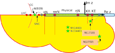
As an illustration of this feature, we give the area of convergence for the P₁₁ partial wave of Jülich model Ronchen2012 as seen by Laurent method in Fig. (1). (Picture is produced on the basis of Fig. (39) of this reference.) The domain of convergence for the Laurent expansion of the Jülich P₁₁ amplitude is indicated in yellow, while the Jülich solution (possibly unknown to us), is valid over the full complex energy plane. We see that the effective area of convergence of the Laurent method is much smaller than the area of convergence of the original model. It is, however, sufficient to enable the analytic continuation of data from the real axis to the nearest singularities. Our aim is not to reproduce the full function, but only the pole parameters of nearby singularities.

Figure 1: (Color online) Domain of convergence of Laurent series for P₁₁ partial wave.

II.2 Pietarinen series

In the following, we propose the use of an expansion, differing from the standard power series for the regular part of Laurent expansion given in Eq.(2). The preferred conformal mapping expansion variable, giving what we call the Pietarinen series, has been proposed and introduced by Ciulli Ciulli ; Ciulli1 and Pietarinen Pietarinen , and it has been used, with great success, in the Karlsruhe-Helsinki partial wave analysis Hoehler84 where invariant amplitudes have been expanded in as many as 50 terms. The aim of this article is not to give the solution in the full complex energy plane which is matching the data, but to give only a locally valid representation of the exact solution, which is however enabling us to extract poles using the data from the real axes. The novelty of our approach is that we propose to avoid discussing the arbitrariness of all possible choices for the background function $B^{L}(\omega)$ by replacing it with rapidly converging Pietarinen power series defined by a complete set of functions with well known analytic properties.

If $F(\omega)$ is a general, unknown analytic function having a cut starting at $\omega=x_{P}$, then using a conformal mapping technique, it can be represented as a power series, having the maximum radius of convergence, in the following way:

$$F(\omega) = \sum_{n=0}^{N}c_{n}\,Z^{n}(\omega),\,\,\,\,\,\,\,\,\,\,\omega\in\mathbb{C}$$

$$Z(\omega) = \frac{\alpha-\sqrt{x_{P}-\omega}}{\alpha+\sqrt{x_{P}-\omega}},\,\,\,\,\,c_{n},x_{P},\alpha\in\mathbb{R},$$ (6)

with the $\alpha$ and $c_{n}$ being tuning parameter and coefficients of Pietarinen function $Z(\omega)$ respectively.

The essence of the approach is the fact that a set $(Z^{n}(\omega),\,n=1,\,\infty)$ forms a complete set of functions defined on the unit circle in the complex energy plane having branch cut starting at $\omega=x_{P}$, but the analytic form of the function is not otherwise defined. The final form of the analytic function $F(\omega)$ is obtained by introducing the rapidly convergent power series with real coefficients, and the degree of the expansion is determined in fitting the input data.

II.3 The application of Pietarinen series to scattering theory

Each partial wave contains poles which identify resonant contributions, and has cuts in the physical region starting at thresholds of elastic and all possible inelastic channels, and finally there are $t$-channel, $u$-channel and nucleon exchange contributions quantified with corresponding negative energy cuts. However, the explicit analytic form of each cut contribution is not known. Instead of guessing the exact analytic form of all of these, we propose to use one Pietarinen series to represent each cut. The number of terms in each Pietarinen series will be determined by the quality of fit to the input amplitudes. In practice, we have too many cuts (especially in the negative-energy range), so we reduce their number by dividing them in two categories: all negative energy cuts are approximated with only one, effective negative energy cut represented with one Pietarinen series, and each physical cut is represented with its own Pietarinen series with branch points determined by the physics of the process.

In summary, the set of equations which define Laurent expansion + Pietarinen series method (L+P method) is:

$$T(\omega) = \sum_{i=1}^{k}\frac{a_{-1}^{(i)}}{\omega_{i}-\omega}+B^{L}(\omega)$$ (7)

$$B^{L}(\omega) = \sum_{n=0}^{M}c_{n}\,Z^{n}(\omega)+\sum_{n=0}^{N}d_{n}\,W^{n}(\omega)+\cdot\cdot\cdot$$

$$Z(\omega) = \frac{\alpha-\sqrt{x_{P}-\omega}}{\alpha+\sqrt{x_{P}-\omega}};\,\,\,\,\,W(\omega)=\frac{\beta-\sqrt{x_{Q}-\omega}}{\beta+\sqrt{x_{Q}-\omega}}+\cdot\cdot\cdot\,\,\,,$$

where $a_{-1}^{(i)},\omega_{i},\omega\in\mathbb{C}$, $c_{n},x_{P},d_{n},x_{Q},\alpha,\beta\in\mathbb{R}$ and ${\rm and}\,\,\,k,M,N\in\mathbb{N}$. All parameters in set the of equations (7) are determined by the fit. As our input data are on the real axis, the fit is performed only on this dense subset of the complex energy plane.

II.4 Fitting procedure

The class of input functions which can conveniently to be analyzed with this method is quite wide. One may either fit partial-wave amplitudes obtained from any theoretical model, or experimental data directly. In either case, the T-matrix is represented by the given set of equations (7), and a minimization criterion (the discrepancy parameter) with respect to the input data is defined (usually $\chi^{2}$ type), and a fit is done. As the partial wave $T$ given by equations (7) does not fulfill the unitarity condition manifestly, we impose elastic unitarity below the first inelastic threshold numerically by introducing a penalty function into the discrepancy parameter of the fit.

We start with minimal number of poles, three Pietarinen functions (one for background, and two for dominant physical channels), and a minimal number of Pietarinen fitting parameters $c_{n},\,d_{n}\,...$ . We usually start with $M,\,N=5$.

The discrepancy parameter is defined as:

$$\chi^{2} = \sum_{j=1}^{N_{pts}}\mid T^{inp}(\omega_{j})-T(\omega_{j})\mid^{2}/{\rm w}_{j}^{2}+\sum_{j=1}^{3}\lambda^{j}\,\chi_{Pen}^{j}+$$ (8)

$$+ \,\Upsilon\,\,\sum_{j=1}^{N_{pts}^{el}}(1-S(\omega_{j})S(\omega_{j})^{\dagger})^{2},$$

where ${\rm w}_{j}$ is the corresponding statistical weight (standard error bar for experimental data and adequate uncertainty parameter for theoretical functions) and $\chi_{Pen}^{j}=\sum_{k=1}^{N}(c_{k}^{j})^{2}\,k^{3}$ is the Pietarinen penalty function Pietarinen which guarantees the soft cut-off of higher order terms in the Pietarinen expansion. The third term in Eq. (8) is introduced to impose elastic unitarity as discussed above. Parameters $\lambda^{j}$ and $\Upsilon$ are penalty function adjusting parameters which serve to bring into correct proportion contributions from penalty functions with the contribution originating from the function itself. They are determined empirically, prior the fit, independently for each penalty function.

The discrepancy parameter is analyzed, and the quality of the fit is also visually inspected by comparing the fitting function with fitted data. If the fit is unsatisfactory (the discrepancy parameter is high, or the fit visually does not reproduce the fitted data), the number of Pietarinen parameters $c_{n},\,d_{n}\,...$ is increased by one. The fit is repeated, and the quality of the fit is re-estimated. This procedure is continued until we have reached a sufficient number of Pietarinen terms so that we are able to reproduce the input data. If the quality of the fit is still unsatisfactory, we first increase the number of poles and then repeat the procedure.

II.5 Limitations of the method

By construction it is clear that the method has its natural limitations. As seen from set of Eqs. (7) our Laurent decomposition contains only two branch points in the physical region, and as seen from Fig.1 this is far from enough in a realistic case. Any realistic analytic function in principle containing more than two branch points will in our model be approximated by a different analytic function containing only two. So, this will be the main source of our errors.

Error analysis will be discussed in detail, in forthcoming publications, when we extract pole positions from experimental data.

III Testing the method

Being aware of the limitations of our method (limited number of branch points), we tested the method in two ways.

First we have tested the method on an elaborate toy model; a model in which we have full control over the analytic structure of the input. We have constructed a toy-model function imitating physical reality as close as possible (known pole parameters, two positive energy cuts and a background contribution), generating the input data table, and verified how well our method reproduces the known input parameters.

However, to prove the applicability of the method in reality, we have tested it on realistic amplitudes as well. We have used our L+P method to extract pole parameters first from several GWU/SAID energy dependent (GWU/SAID ED) $\pi$N elastic partial wave amplitudes with known (published) pole positions GWU ; GWU1 , and also on the Dubna-Mainz-Taipei energy dependent (DMT ED) DMT0 ; DMT amplitudes. Exploring GWU/SAID pole structure is the first analysis of these amplitudes by the present collaboration, while Zagreb-Mainz-Taipei collaboration have already used DMT amplitudes for testing other possible single channel, but local, pole extraction methods such as the speed plot (SP), renormalization method, etc. For further details we refer the reader to reference DMT0 ; DMT . We consider it important to mention that DMT amplitudes have more poles than have been reported in DMT0 ; DMT , and we use them in our analysis as well DMT1 . Included here are the S₁₁, S₃₁ P₁₁, D₁₃, D₃₃, F₁₅ and F₃₇ amplitudes. We expect that the agreement with ”exact” results, obtained by analytic continuation of known functions into the complex energy plane, will be poorer than in the toy-model case, as each model has its own complicated analytic structure, and fitting with two branch points only will definitely influence pole positions. However, we show that the results in these cases are very good as well.

Finally let us also mention that analytical continuations of K-matrix and/or dynamical models are also not absolutely free of uncertainties. There are various elaborate numerical methods, which are not always free of numerical instabilities. This is especially true when poles are very far away from the physical axis or when the structure of Riemann sheets in the models becomes complicated.

III.1 Fitting the toy-model

Table 1: Toy model parameters and fitted parameters. Input parameters are given in boldface, and results of a fit in normal font. Table is given in GeV units. $\alpha,\beta$ , and $\gamma$ are tuning parameters in corresponding Pietarinen functions.

	$r_{1}$	$g_{1}$	$M_{1}$	$\Gamma_{1}$	$r_{2}$	$g_{2}$	$M_{2}$	$\Gamma_{2}$	$\alpha$	$x_{P}$	$N_{1}$	$\beta$	$x_{Q}$	$N_{2}$	$\gamma$	$x_{R}$	$N_{3}$	$10^{2}\chi_{R}^{2}$
Toy-model
	0.1	0.09	1.65	0.165	0.09	0.06	2.25	0.2
Fitted results
P1	0.085	0.102	1.663	0.171	0.087	0.075	2.262	0.216	1.09	-2.64	10							328.19
P2	0.098	0.086	1.650	0.161	0.095	0.058	2.247	0.199	0.44	-0.47	9	1.95	3.97	8				70.37
P3	0.099	0.090	1.650	0.164	0.089	0.061	2.251	0.200	4.19	-22.99	5	2.22	3.98	5	1.67	0.97	3	0.24

In principle, we could have defined toy-model input data $T^{ty}(\omega_{j})$ by defining a toy-model function and by normally distributing its values in order to simulate the statistical nature of real measured data. However, as the main goal of this paper is to establish the validity of the approach, we have restricted our analysis to infinitely precise data by using non-distributed toy-function values, and using a statistical weight ${\rm w}_{j}$ of 5 %.
Our toy-model function is constructed by assuming a typical analytic structure of a partial wave: it is constructed as a sum of two poles, two physical cuts and several non-resonant background contributions. The function representing physical cuts is constructed from a function $f(x,a)=\sqrt{x^{2}-4ax}/2x$ having a cut starting from $x_{0}=4a$ on the real axes, and the analyticity is imposed through the once subtracted dispersion relation $\Phi(x,a)=\frac{x-x_{0}}{\pi}\int_{x_{0}}^{\infty}\frac{f(x^{\prime},a)}{(x^{\prime}-x)(x^{\prime}-x_{0})}\,dx^{\prime}$. However, to simplify our demonstration of utility of the L+P method, we replace all negative energy cuts with two poles deep in unphysical region. In spite of appearing rather restrictive, such an approximation is reasonably justified. Namely, we know that each cut can be represented by the infinite sum of poles, and as negative cut is indeed very far from the region of interest, replacing it with only two out of infinite number of poles is a good approximation (see Cutkosky CMB approach CMB ).

Thus our toy-model function is given as:

$$T^{ty}(\omega) = \sum_{k=1}^{2}\frac{r_{k}+i\,\,g_{k}}{M_{k}-\omega-i\,\,\Gamma_{k}/2}+$$

$$+ \Phi(\omega,0.25)+\Phi(\omega,1.)+B(\omega),$$

$$\Phi(\omega,a) = \frac{\sqrt{\omega(-4a+\omega)}}{2\pi\omega}\ln\frac{{2a-\omega-\sqrt{\omega(-4a+\omega)}}}{2a}$$

$$B(\omega) = \frac{10.}{-10.-\omega-i\,\,5.}+\frac{10.}{-6.-\omega-i\,\,4.},$$

where $r_{k},g_{k},M_{k},\Gamma_{k}\in\mathbb{R}$.

Toy-model parameters for all test cases are chosen to resemble physical reality as much as possible, and are given in Table 1 with bold face characters. By construction, our toy-model function has two poles and two cuts producing clearly visible pole structure and two pronounced cusps at 1.0 GeV ($a=0.25$ GeV) and 4.0 GeV ($a=1.00$ GeV).

Results of the fit for all cases are given in Table 1 and Fig. 2. For more numerical parameters we refer the reader to the reference Svarc2012 where an expanded version of the toy-model is given.

Figure 2: (Color online) Toy-model function. Dashed-dotted, dashed and full lines P1, P2 and P3 give the quality of the fit for solutions with one, two and three Pietarinen expansions respectively.

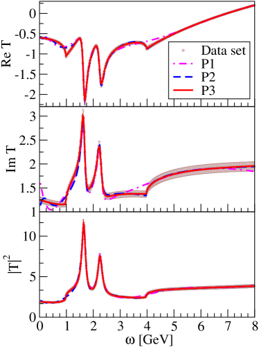
In conclusion, we claim that the basic assumptions of the approach have been confirmed. All pole parameters are almost exactly reproduced. The Pietarinen branch point $x_{P}$ turns out to be subthreshold and effectively reproduces background contributions, and Pietarinen branch points $x_{Q}$ and $x_{R}$ correspond to the branchpoints of the toy-model function (1. and 4.).

We have also tested the dependence of the fitting success upon the number of Pietarinen series used.

In Table 1 and Fig. 2, we show a fit the full model only with one Pietarinen (P1), two Pietarinens (P2) and three Pietarinen series (P3). It is straightforward to see that if one uses only one expansion, reduced $\chi^{2}$ ($\chi^{2}_{R}$ - discrepancy parameter per degree of freedom) is high (3.2819), and the fitting function ”misses” both cusps. When the number of Pietarinen series raises to two (P2), reduced $\chi^{2}$ is improved (0.7037) and one cusp (higher one at 4) is covered, so we indeed need all three Pietarinen series (P3) to reproduce all poles and all cusps and obtain the best reduced $\chi^{2}=0.0024$. We note that the very small $\chi^{2}$ is a measure of the goodness of our fit only. It is not a $\chi^{2}$ in a statistical sense, because the input ”data” are not statistically distributed with standard error definition, but taken from a numerical function with an arbitrary error of 5% being assumed. In the final case, where the number of Pietarinen series corresponded to the number of cuts, all pole parameters perfectly corresponded to the toy-model input values.

III.2 Fitting the realistic input

The L+P method allows the extraction of poles from partial waves obtained as result of theoretical analysis (”theoretical input”) and, we have used it to extract poles from GWU/SAID and DMT $\pi$N elastic amplitudes. However, if the ”theoretical input” has analytic structure in the regular part different from the cut structure assumed in the fit, errors in fitting the background will be transferred to pole parameters, as the fit will try to compensate.

We apply the following strategy:

1) We fix the pion-nucleon elastic threshold position at the experimental value, and
2) Allow other threshold positions to vary as a parameters in a fit and find optimal values which replace exact physical thresholds.

Figure 3: (Color online) L+P fit to partial waves from Fa02 solution. Dashed blue line and solid red line show fit to real and imaginary parts of partial waves, respectively.

Figure 4: (Color online) L+P fit to partial waves from Sp06 solution. Dashed blue line and solid red line show fit to real and imaginary parts of partial waves, respectively.

Figure 5: (Color online) L+P to partial waves from Wi08 solution. For D₃₃ partial wave we have no values for poles, so we omitted it from fitting. Dashed blue line and solid red line show fit to real and imaginary parts of partial waves, respectively.

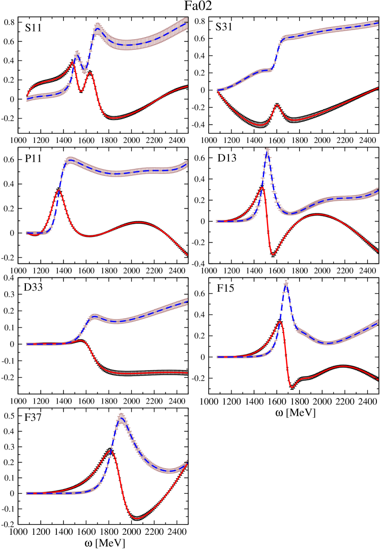
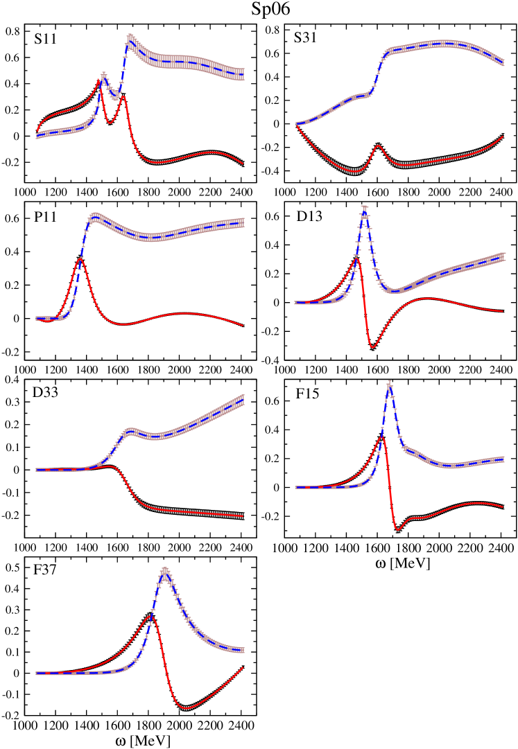
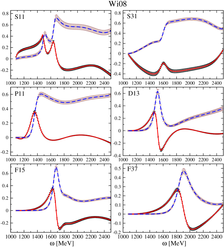
Comparison of results from L+P fit and values from original publications is given in Tables II and III. Instead of real and imaginary parts of residua, in Table II we give their modula $|a_{i}|$ and corresponding phases $\theta_{i}$. $x_{P},x_{Q}$ and $x_{R}$ denote threshold positions in corresponding Pietarinen series. As it may be seen from the Tables II and III results obtained from L+P agree very well with published values GWU ; GWU1 , and DMT0 ; DMT ; DMT1 . The quality of the fit to the input is given in Figs. (3)-(6).

Table 2: Comparison of GWU/SAID ED pole positions with values obtained by L+P method. Table is given in MeV units, and $\Gamma_{i}=-2\,\omega_{i}$.

PW	Solution	$M_{1}$	$\Gamma_{1}$	$|a_{1}|$	$\theta_{1}^{0}$	$M_{2-4}$	$\Gamma_{2-4}$	$|a_{2-4}|$	$\theta_{2-4}^{0}$	$x_{P}$/103	$x_{Q}$/103	$x_{R}$/103	$10^{2}\chi_{R}^{2}$
	FA02 GWU	1526	130	33	14	1653	182	69	-55
S11	FA02 L+P	1518	121	17	-32	1656	182	68	-39	-60.1	1.077	1.471	0.32
	SP06 GWU	1502	95	16	-16	1648	80	14	-69
	SP06 L+P	1509	96	15	-21	1645	80	14	-80	-29.5	1.077	1.479	2.90
	WI08 GWU1	1499	98	-	-	1647	84	-	-
						1666	520	-	-
	WI08 L+P	1504	78	11	-60	1644	86	17	-83
						1669	517	419	-74	-0.339	1.077	1.483	3.57
	FA02 GWU	1594	118	17	-104
S31	FA02 L+P	1596	112	15	-101					-59.3	1.077	1.183	0.48
	SP06 GWU	1595	135	15	-92
	SP06 L+P	1596	133	18	-105					-16.7	1.077	1.309	0.35
	WI08 GWU1	1594	136	-	-
	WI08 L+P	1598	130	18	-104					-92.7	1.077	1.589	0.57
	FA02 GWU	1357	160	36	-102
P11	FA02 L+P	1354	169	38	-98					-100	1.077	1.202	0.66
	SP06 GWU	1359	162	38	-98
	SP06 L+P	1358	183	53	-92					-62.1	1.077	1.215	0.09
	WI08 GWU1	1358	160	-	-
	WI08 L+P	1357	177	47	-93					-98.9	1.077	1.202	0.07
	FA02 GWU	1514	102	35	-6
D13	FA02 L+P	1513	101	34	-9					-67.4	1.077	1.222	0.85
	SP06 GWU	1515	113	38	-5
	SP06 L+P	1515	113	38	-6					-50.1	1.077	1.216	0.57
	WI08 GWU1	1515	110	-	-
	WI08 L+P	1515	111	38	-5					-81.1	1.077	1.169	0.15
	FA02 GWU	1617	226	16	-47
D33	FA02 L+P	1618	227	16	-47					-27.3	1.077	1.204	0.008
	SP06 GWU	1632	253	18	-48
	SP06 L+P	1635	251	18	-37					-54.1	1.077	1.198	0.009
	WI08 GWU1	no results
	WI08 L+P
	FA02 GWU	1678	120	43	1	1779	248	47	-61
F15	FA02 L+P	1679	118	42	-5	1779	245	31	-84	1.032	1.077	1.549	0.64
	SP06 GWU	1674	115	42	-4	1785	244	60	-67
	SP06 L+P	1673	116	43	-14	1776	226	24	-98	-8.99	1.077	1.301	0.08
	WI08 GWU1	1674	114	-	-	1779	276	-	-
	WI08 L+P	1675	115	44	-8	1776	233	34	-99	-51.7	1.077	1.726	0.28
	FA02 GWU	1874	236	57	-34
F37	FA02 L+P	1874	236	55	-35					-14.9	1.077	1.739	0.04
	SP06 GWU	1876	227	53	-31
	SP06 L+P	1876	226	53	-31					-32.8	1.077	1.137	0.06
	WI08 GWU1	1883	230	-	-
	WI08 L+P	1874	227	55	-35					-37.8	1.077	1.736	0.03

Table 3: Comparison of DMT ED pole positions with values obtained by L+P method. Table is given in MeV units, and $\Gamma_{i}=-2\,\omega_{i}$.

PW	Solution	$M_{1}$	$\Gamma_{1}$	$|a_{1}|$	$\theta_{1}^{0}$	$M_{2-4}$	$\Gamma_{2-4}$	$|a_{2-4}|$	$\theta_{2-4}^{0}$	$x_{P}$/103	$x_{Q}$ /103	$x_{R}$/103	$10^{2}\chi_{R}^{2}$
S11	DMT DMT0 ; DMT	1499	78	14	-45	1631	120	35	-83
						1733	180	16	-29
	DMT DMT1					2027	180	23	-150
	DMT L+P	1500	76	13.4	-46	1636	99	22	-94
						1810	164	9.6	-176
						2077	220	22.5	-122	1.0	1.077	1.486	0.6
S31	DMT DMT0 ; DMT	1598	148	23	-98	1774	72	3.8	-181
						1984	254	26	-170
	DMT L+P	1597	140	21	-104	1771	69	2.2	-172
						2040	195	7	-109	-11.476	1.077	1.739	0.2
P11	DMT DMT0 ; DMT	1371	190	50	-79	1746	368	11	-54
	DMT DMT1					1997	458	56	-145
	DMT L+P	1370	190	50	-81	1763	235	5	-56
						2015	467	36	-99	0.699	1.077	1.537	0.05
D13	DMT DMT0 ; DMT	1515	120	40	-7	1718	96	2.8	-91
						1854	214	16	-96
	DMT DMT1					2099	216	13	-58
	DMT L+P	1517	120	40	-5	1721	89	2.1	-76
						1858	228	15	-87
						2101	231	14	-49	1.00	1.077	1.266	0.32
D33	DMT DMT0 ; DMT ; DMT1	1604	142	9.4	-63	2042	254	4.84	-75
	DMT L+P	1605	141	9.3	-63	2023	241	4	-93	0.623	1.077	1.324	0.06
F15	DMT DMT0 ; DMT	1664	114	38	-26	1919	52	1.0	15
	DMT L+P	1664	114	38	-26	1920	52	1.0	16	0.7	1.077	1.225	0.02
F37	DMT DMT0 ; DMT	1858	208	43	-48
	DMT L+P	1858	207	43	-49					-3.999	1.077	1.223	0.48

Figure 6: (Color online) L+P to partial waves from DMT solution. Dashed blue line and solid red line show fit to real and imaginary parts of partial waves, respectively.

IV Results and Discussion

IV.1 General considerations

By using Laurent expansion near real axes, and Pietarinen series to constrain unknown regular part, we have been able to extract pole parameters in all test cases where the pole parameters have been known by using other methods without exemption, and our value corresponded to the know input fairly well.

IV.1.1 Toy-model

First we tested the toy-model where the analytic structure was known, and relatively simple. The agreement given in Table 1 is below 1 %.

IV.1.2 GWU/SAID ED solutions

To illustrate the applicability of the method to situations where the analytic structure of the input is much more complicated, and we are approximating the complicated input analytic function with simpler one, we have tested two sets of ED amplitudes; GWU/SAID GWU ; GWU1 , and DMT DMT . We have compared only those partial waves for which the input pole parameters are explicitly published.

Results for GWU/SAID amplitude are give in Table 2, and in Figs. (3)-(5). The GWU/SAID fit uses a Chew-Mandelstam K-matrix model and the resulting T-matrix poles are not generally included as explicit K-matrix poles. In addition, the model employs complex branch points for the opening $\pi\Delta$ and $\rho N$ channels. Given these complications, we anticipated that the analytic structure of the regular part could be rather complicated, and we would have some problems in fitting these amplitudes within our method. This expectation is confirmed. In spite of an almost ideal ability of our simpler background to reproduce the more complicated input, demonstrated by extremely good fits given in Figs. (3)-(5), and low $\chi^{2}$ parameter given in Table 2, some differences in pole parameters should and do occur. However, we state:

• the quality of the fit is ideal (see Figs. 3, 4 and 5)

• we find an identical number of poles as the GWU/SAID group

• we are able to follow the significant change of pole positions, due to slight changes of input, as reported by the GWU/SAID group (the input for the S11 partial wave is only modestly modified at higher energies between the FA02 and SP06 solutions, but the change in width of the S11(1650) resonance is noticeable: from 182 MeV for FA02 to 80 for SP06. We reproduce this finding.)

• our agreement for the lowest partial waves is in principle better than 10 % for lower resonances, and only slightly worse for higher ones

• our L+P method disagreed with the GWU/SAID pole position published for the second F15 resonance, and this revealed a missprint in the original publication (see footnote in Table 2).

IV.1.3 DMT ED solutions

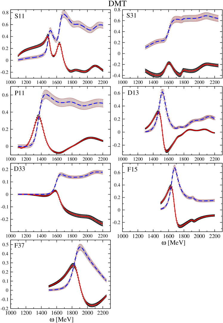
As the DMT model is a T-matrix model, we expect that its analytic structure will be much easier to reconstruct for the L+P model, so we expect better results. It is based on a $\pi N$ meson exchange model and describes $\pi N$ phase shifts and inelasticity parameters in all the partial waves up to the F waves and energies of $W=2$ GeV. It is a dynamical model with $\pi N$, $2\pi N$ and $\eta N$ coupled channels, leading to a simpler branch point structure than the GWU/SAID K-matrix approach or more sophisticated dynamical models with many more coupled channels and complex branch points Ronchen2012 . Most resonances are included as bare resonances which get dressed by the dynamically calculated self-energies, and the pole positions and residues can be calculated by analytical continuation into the complex region. In addition, like in all dynamical models, dynamically generated poles can be found, most of them far away form the physical axis. The results and the quality of the fit is shown in Table 3. We state:

• the quality of the fit is ideal (see Fig. 6)

• we find the same number of poles as DMT group DMT

• our L+P method disagrees with the DMT published pole position for the second P11 resonance, where we observe a $30\%$ deviation in the pole width and a $50\%$ deviation in the residue. However, this pole has the smallest ”normalized residue”, defined as $R_{norm}=Res/(\Gamma/2)$, from all resonances in Table 3. Its value is only $6\%$ whereas the largest one in the table is found for the $D_{13}(1520)$ with $67\%$. Also small values are found for the third $S_{11}$ ($18\%$), the second $S_{31}$ ($11\%$) and second, third and fourth $D_{13}$ ($6\%$, $15\%$ and $12\%$, respectively). Quantitatively, we observe larger deviations as smaller the reduced residues get. This quantity is a very good measure for the strength and importance of a resonance, the maximum value among all nucleon resonances is obtained for the $\Delta(1232)$ with $100\%$.

IV.2 GWU/SAID P₁₁ poles in ED and single energy solutions (SES)

Figure 7: (Color online) Comparison beetween GWU-SES, GWU-SP06 and Karlsruhe-Helsinki KH80 Hoehler84 solution for P11 partial wave.

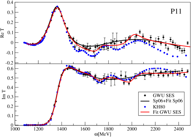
In order to demonstrate the importance and novelty of extracting poles from amplitudes more closely associated with experimental data using L+P method, we have extracted poles from the $P_{11}$ partial wave of the GWU/SAID SES, and have compared these with results using the ED GWU/SAID fit SP06. The results are interesting. However, before discussing this fit, it is useful to recall how the SES fits differ (and are related to) the ED fits.

The SES amplitudes come from fits to data within narrow windows of energy. The energy variation over each range is determined by the underlying ED fit. However, as each fit is done independently, there is no smoothness constraint applied to the set of resulting SES. Dispersion relation constraints are also omitted in these fits, which were done initially to search for systematic variations, possibly signaling missing structure. Having obtained these SES, there is an element of subjectivity in assessing whether the variations are random or indicative of missing (possibly resonant) structure. In the case of the P₁₁ amplitude, other analyses (both multi-channel and elastic) have suggested the existence of several P₁₁ states, whereas the GWU/SAID fits find only the single (Roper) resonance $N(1440)$. As no explicit pole is added in the fit, the Roper has been found in a search of the complex energy plane.

The P₁₁ amplitude is complicated by the existence of the $\pi\Delta$ branch point very near the first resonance pole. The amplitude, plotted in an Argand diagram, also stays near its center for energies spanning the whole resonance region beyond the Roper, which hinders the determination of phase (looping) behavior. Several attempts have been made to add structure GWU1 ; VPI either by inserting resonances by hand, adding soft pseudo-data constaints based on the KH80 Hoehler84 and CMB CMB amplitudes, or adding an extra explicit pole to each partial wave via the Chew-Mandelstam K-matrix. In the latter attempt, a second pole was extracted but its position was not comparable to other determinations. A comparison of the GWU/SAID SES and the much older KH80 fit is suggestive as KH80 finds a second resonance and seems to follow all the structure seen in the SES.

We can fit both the ED and SES solutions. The quality of the fit is shown in Fig. (7). However, we need three poles for GWU-SES, but need only one pole for SP06. We have tried fitting SP06 with two poles, but the the second pole turned out to be completely undetermined. However, when fitting GWU-SES as input, the existence of the second pole is definitely established, and the existence of the third pole is very likely. These results are very similar to what GWU group claims: P${}_{11}(1710)$ is not found in the complex plane of the ED analysis.
Our results are:

• GWU-SP06
                  $P_{1}^{\rm SP06}=1.358-i\>0.0915$

• GWU-SES

  $$P_{1} = 1.362-i\>0.0895,$$

  $$P_{2} = 1.716-i\>0.0495,$$

  $$P_{3} = 1.999-i\>0.0715.$$

Using the L+P method allows us to see P${}_{11}(1710)$ and P${}_{11}(2100)$ in the GWU-SES, while GWU/SAID energy dependent analysis does not contain this additional structure. It would be interesting to see if, by adding further explicit poles, this result could be found also in the GWU/SAID ED approach.