A 325-MHz GMRT survey of the Herschel-ATLAS/GAMA fields

Abstract

We describe a 325-MHz survey, undertaken with the Giant Metrewave Radio Telescope (GMRT), which covers a large part of the three equatorial fields at 9, 12 and 14.5 h of right ascension from the Herschel-Astrophysical Terahertz Large Area Survey (H-ATLAS) in the area also covered by the Galaxy And Mass Assembly survey (GAMA). The full dataset, after some observed pointings were removed during the data reduction process, comprises 212 GMRT pointings covering $\sim 90$ deg² of sky. We have imaged and catalogued the data using a pipeline that automates the process of flagging, calibration, self-calibration and source detection for each of the survey pointings. The resulting images have resolutions of between 14 and 24 arcsec and minimum rms noise (away from bright sources) of $\sim 1$ mJy beam^-1, and the catalogue contains 5263 sources brighter than $5\sigma$. We investigate the spectral indices of GMRT sources which are also detected at 1.4 GHz and find them to agree broadly with previously published results; there is no evidence for any flattening of the radio spectral index below $S_{1.4}=10$ mJy. This work adds to the large amount of available optical and infrared data in the H-ATLAS equatorial fields and will facilitate further study of the low-frequency radio properties of star formation and AGN activity in galaxies out to $z\sim 1$.

1 Introduction

The Herschel-Astrophysical Terahertz Large Area Survey (H-ATLAS; Eales et al., 2010) is the largest Open Time extragalactic survey being undertaken with the Herschel Space Observatory (Pilbratt et al., 2010). It is a blind survey and aims to provide a wide and unbiased view of the sub-millimetre Universe at a median redshift of $1$. H-ATLAS covers $\sim 570$ deg² of sky at $110$, $160$, $250$, $350$ and $500$ ${\mu}$m and is observed in parallel mode with Herschel using the Photodetector Array Camera (PACS; Poglitsch et al., 2010) at 110 and 160 ${\mu}$m and the Spectral and Photometric Imaging Receiver (SPIRE; Griffin et al., 2010) at 250, 350 and 500 ${\mu}$m. The survey is made up of six fields chosen to have minimal foreground Galactic dust emission, one field in the northern hemisphere covering $150$ deg² (the NGP field), two in the southern hemisphere covering a total of $250$ deg² (the SGP fields) and three fields on the celestial equator each covering $\sim 35$ deg² and chosen to overlap with the Galaxy and Mass Assembly redshift survey (GAMA; Driver et al., 2011) (the GAMA fields). The H-ATLAS survey is reaching 5-$\sigma$ sensitivities of (132, 121, 33.5, 37.7, 44.0) mJy at (110, 160, 250, 350, 500) $\mu$m and is expected to detect $\sim 200,000$ sources when complete (Rigby et al., 2011).

A significant amount of multiwavelength data is available and planned over the H-ATLAS fields. In particular, the equatorial H-ATLAS/GAMA fields, which are the subject of this paper, have been imaged in the optical (to $r\sim 22.1$) as part of the Sloan Digital Sky Survey (SDSS; York et al., 2000) and in the infrared (to $K\sim 20.1$) with the United Kingdom Infra-Red Telescope (UKIRT) through the UKIRT Infrared Deep Sky Survey (UKIDSS; Lawrence et al., 2007) Large Area Survey (LAS). In the not-too-distant future, the GAMA fields will be observed approximately two magnitudes deeper than the SDSS in 4 optical bands by the Kilo-Degree Survey (KIDS) to be carried out with the Very Large Telescope (VLT) Survey Telescope (VST), which was the original motivation for observing these fields. In addition, the GAMA fields are being observed to $K\sim 1.5-2$ mag. deeper than the level achieved by UKIDSS as part of the Visible and Infrared Survey Telescope for Astronomy (VISTA) Kilo-degree Infrared Galaxy (VIKING) survey, and with the Galaxy Evolution Explorer (GALEX) to a limiting AB magnitude of $\sim 23$.

In addition to this optical and near-infrared imaging there is also extensive spectroscopic coverage from many of the recent redshift surveys. The SDSS survey measured redshifts out to $z\sim 0.3$ in the GAMA and NGP fields for almost all galaxies with $r<17.77$. The Two-degree Field (2dF) Galaxy Redshift Survey (2dFGRS; Colless et al., 2001) covers much of the GAMA fields for galaxies with $b_{J}<19.6$ and median redshift of $\sim 0.1$. The H-ATLAS fields were chosen to overlap with the GAMA survey, which is ongoing and aims to measure redshifts for all galaxies with $r<19.8$ to $z\sim 0.5$. Finally, the WiggleZ Dark Energy survey has measured redshifts of blue galaxies over nearly half of the H-ATLAS/GAMA fields to a median redshift of $z\sim 0.6$ and detects a significant population of galaxies at $z\sim 1$.

The wide and deep imaging from the far infrared to the ultraviolet and extensive spectroscopic coverage makes the H-ATLAS/GAMA fields unparallalled for detailed investigation of the star-forming and AGN radio source populations. However, the coverage of the H-ATLAS fields is not quite so extensive in the radio. All of the fields are covered down to a $5\sigma$ sensitivity of 2.5 mJy beam^-1 at 1.4 GHz by the National Radio Astronomy Obervatory (NRAO) Very Large Array (VLA) Sky Survey (NVSS; Condon et al., 1998). These surveys are limited by their $\sim 45$-arcsec resolution, which makes unambiguous identification of radio sources with their host galaxy difficult, and by not being deep enough to find a significant population of star-forming galaxies, which only begin to dominate the radio-source population below 1 mJy (e.g. Wilman et al., 2008). The Faint Images of the Radio Sky at Twenty-cm (FIRST; Becker et al., 1995) survey covers the NGP and GAMA fields at a resolution of $\sim 6$ arcsec down to $\sim 0.5$ mJy at 1.4 GHz, is deep enough to probe the bright end of the star-forming galaxy population, and has good enough resolution to see the morphological structure of the larger radio-loud AGN, but it must be combined with the less sensitive NVSS data for sensitivity to extended structure. Catalogues based on FIRST and NVSS have already been used in combination with H-ATLAS data to investigate the radio-FIR correlation (Jarvis et al., 2010) and to search for evidence for differences between the star-formation properties of radio galaxies and their radio-quiet counterparts (Hardcastle et al. 2010, 2012; Virdee et al. 2013).

To complement the already existing radio data in the H-ATLAS fields, and in particular to provide a second radio frequency, we have observed the GAMA fields (which have the most extensive multi-wavelength coverage) at 325 MHz with the Giant Metrewave Radio Telescope (GMRT; Swarup et al., 1991). The most sensitive GMRT images reach a $1\sigma$ depth of $\sim 1$ mJy beam^-1 and the best resolution we obtain is $\sim 14$ arcsec, which is well matched to the sensitivity and resolution of the already existing FIRST data. The GMRT data overlaps with the three $\sim 60$-deg² GAMA fields, and cover a total of $108$ deg² in $288$ 15-minute pointings (see Fig. 2). These GMRT data, used in conjunction with the available multiwavelength data, will be valuable in many studies, including an investigation of the radio-infrared correlation as a function of redshift and as a function of radio spectral index, the link between star formation and accretion in radio-loud AGN and how this varies as a function of environment and dust temperature, and the three-dimensional clustering of radio-source populations. The data will also bridge the gap between the well-studied 1.4-GHz radio source populations probed by NVSS and FIRST and the radio source population below 250 MHz, which will be probed by the wide area surveys made with the Low Frequency Array (LOFAR; Röttgering et al., 2006) in the coming years.

This paper describes the 325-MHz survey of the H-ATLAS/GAMA regions. The structure of the paper is as follows. In Section 2 we describe the GMRT observations and the data. In Section 3 we describe the pipeline that we have used to reduce the data and in Section 4 we describe the images and catalogues produced. In Section 5 we discuss the data quality and in Section 6 we present the spectral index distribution for the detected sources between 1.4 GHz and 325 MHz. A summary and prospects for future work are given in Section 7.

2 GMRT Observations

Table 1: Summary of the GMRT observations.

Date	Start Time (IST)	Hours Observerd	Nantennas	Antennas Down	Comments
2009, Jan 15	21:00	14.0	27	C01,S03,S04	C14,C05 stopped at 09:00
2009, Jan 16	21:00	15.5	27	C01,S02,S04	C04,C05 stopped at 09:00
2009, Jan 17	21:00	15.5	29	C01	C05 stopped at 06:00
2009, Jan 18	21:00	16.5	26	C04,E02,E03,E04	C05 stopped at 09:00
2009, Jan 19	22:00	16.5	29	C04
2009, Jan 20	21:00	13.5	29	C01	20min power failure at 06:30
2009, Jan 21	21:30	13.0	29	S03	Power failure after 06:00
2010, May 17	16:00	10.0	26	C12,W01,E06,E05
2010, May 18	17:00	10.0	25	C11,C12,S04,E05,W01	E05 stopped at 00:00
2010, May 19	18:45	10.5	25	C12,E05,C05,E03,E06	40min power failure at 22:10
2010, Jun 4	13:00	12.0	28	W03,W05

2.1 Survey Strategy

The H-ATLAS/GAMA regions that have been observed by the Herschel Space Observatory and are followed up in our GMRT survey are made up of three separate fields on the celestial equator. The three fields are centered at 9 h, 12 h, and 14.5 h right ascension (RA) and each spans approximately 12 deg in RA and 3 deg in declination to cover a total of 108 deg² (36 deg² per field). The Full Width at Half Maximum (FWHM) of the primary beam of the GMRT at 325 MHz is 84 arcmin. In order to cover each H-ATLAS/GAMA field as uniformly and efficiently as possible, we spaced the pointings in an hexagonal grid separated by 42 arcmin. An example of our adopted pointing pattern is shown in Fig. 1; each field is covered by 96 pointings, with 288 pointings in the complete survey.

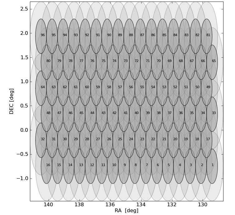
Figure 1: The 96 hexagonal GMRT pointings for the 9-h H-ATLAS/GAMA fields. The pointing strategy for the 12- and 14.5-h fields is similar. The dark grey ellipses (circles on the sky) show the 42-arcmin region at the centre of each pointing; the light grey ellipses (circles) show the 84-arcmin primary beam.

2.2 Observations

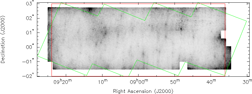
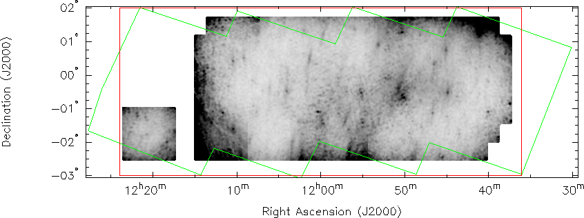
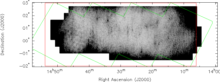
Figure 2: Coverage and rms noise maps for the three survey fields. For all three fields, the greyscale runs from 0 (white) to 6 mJy beam^-1 (black). White areas were not covered by the survey, either intentionally or due to loss of data due to RFI or other instrumental problems. The overplotted red boxes show the GAMA survey areas and the green lines denote the boundary of the H-ATLAS observations.

Figure 3: Left: Typical $uv$ coverage of a survey pointing. This shows the $uv$ coverage of the pointing PNC71 (see Section 4.2 for an explanation of this notation) which had $2\times 7.5$ minute scans, separated by 3.5 h. Right: The dirty beam corresponding to the $uv$ coverage on the right, with robust weighting. Contours are plotted at 80, 60, 40, 15, 8, 2, $-$2 and $-$5 per cent of the peak.

Observations were carried out in three runs in Jan 2009 (8 nights) and in May 2010 (3 nights) and in June 2010 (1 night). Table 1 gives an overview of each night’s observing. On each night as many as 5 of the 30 GMRT antennas could be offline for various reasons, including being painted or problems with the hardware backend. On two separate occasions (Jan 20 and May 19) power outages at the telescope required us to stop observing, and on one further occasion on Jan 21 a power outage affected all the GMRT baselines outside the central square. Data taken during the Jan 21 power outage were later discarded.

Each night’s observing consisted of a continuous block of 10-14 h beginning in the early evening or late afternoon and running through the night. Night-time observations were chosen so as to minimise the ionopheric variations. We used the GMRT with its default parameters at 325 MHz and its hardware backend (GMRT Hardware Backend; GHB), two 16 MHz sidebands (Upper Sideband; USB, and Lower Sideband; LSB) on either side of 325 MHz, each with 128 channels, were used. The integration time was set to 16.7 s.

The flux calibrators 3C147 and 3C286 were observed for 10 minutes at the beginning and towards the end of each night’s oberving. We assumed 325-MHz flux densities of 46.07 Jy for 3C 147 and 24.53 Jy for 3C 286, using the standard VLA (2010) model provided by the AIPS task SETJY. Typically the observing on each night was divided into 3 $\sim 4-5$-h sections, concentrating on each of the 3 separate fields in order of increasing RA. The 9-h and 12-h fields were completely covered in the Jan 2009 run and we carried out as many observations of the 14.5-h field as possible during the remaining nights in May and June 2010. The resulting coverage of the sky, after data affected by power outages or other instrumental effects had been taken into account, is shown in Fig. 2, together with an indication of the relationship between our sky coverage and that of GAMA and H-ATLAS.

Each pointing was observed for a total of 15 minutes in two 7.5-min scans, with each scan producing $\sim 26$ records using the specified integration time. The two scans on each pointing were always separated by as close to 6 h in hour angle as possible so as to maximize the $uv$ coverage for each pointing. The $uv$ coverage and the dirty beam of a typical pointing, observed in two scans with an hour-angle separation of 3.5 h, is shown in Fig. 3.

2.3 Phase Calibrators

One phase calibrator near to each field was chosen and was verified to have stable phases and amplitudes on the first night’s observing. All subsequent observations used the same phase calibrator, and these calibrators were monitored continuously during the observing to ensure that their phases and amplitudes remained stable. The positions and flux densities of the phase calibrators for each field are listed in Table 2. Although there are no 325-MHz observations of the three phase calibrators in the literature, we estimated their 325-MHz flux densities that are listed in the table using their measured flux densities from the 365-MHz Texas survey (Douglas et al., 1996) and extrapolated to 325 MHz assuming a spectral index of $\alpha=-0.8$.

Each 7.5-minute scan on source was interleaved with a 2.5-minute scan on the phase calibrator in order to monitor phase and amplitude fluctuations of the telescope, which could vary significantly during an evening’s observing. During data reduction we discovered that the phase calibrator for the 14.5-h field (PHC00) was significantly resolved on scales of $\sim 10$ arcsec. It was therefore necessary to flag all of the data at $uv$ distance $>20$ k$\lambda$ from the 14.5-h field. This resulted in degraded resolution and sensitivity in the 14.5-h field, which will be discussed in later sections of this paper.

During observing the phases and amplitudes of the phase calibrator measured on each baseline were monitored. The amplitudes typically varied smoothly by $<30$ per cent in amplitude for the working long baselines and by $<10$ per cent for the working short baselines. We can attribute some of this effect to variations in the system temperature, but since the effects are larger on long baselines it may be that slight resolution of the calibrators is also involved. Phase variations on short to medium baselines were of the order of tens of degrees per hour, presumably due to ionospheric effects. On several occasions some baselines showed larger phase and amplitude variations, and these data were discarded during the data reduction.

Table 2: The phase calibrators for the three fields.

Calibrator	Field	RA (J2000)	Dec. (J2000)	$S_{325\,{\rm MHz}}$
Name		hh mm ss.ss	dd mm ss.ss	Jy
PHA00	9-hr	08 15 27.81	-03 08 26.51	9.3
PHB00	12-hr	11 41 08.24	+01 14 17.47	6.5
PHC00	14.5-hr	15 12 25.35	+01 21 08.64	6.7

3 The Data Reduction Pipeline

The data handling was carried out using an automated calibration and imaging pipeline. The pipeline is based on python, aips and ParselTongue (Greisen 1990; Kettenis 2006) and has been specially developed to handle GMRT data. The pipeline performs a full cycle of data calibration, including automatic flagging, delay corrections, absolute amplitude calibration, bandpass calibration, a multi-facet self-calibration process, cataloguing, and evaluating the final catalogue. A full description of the GMRT pipeline and the calibration will be provided elsewhere (Klöckner in prep.).

3.1 Flagging

The GMRT data varies significantly in quality over time; in particular, some scans had large variations in amplitude and/or phase over short time periods, presumably due either to instrumental problems or strong ionospheric effects. The phases and amplitudes on each baseline were therefore initially inspected manually and any scans with obvious problems were excluded prior to running the automated flagging procedures. Non-working antennas listed in Table 1 were also discarded at this stage. Finally, the first and last 10 channels of the data were removed as the data quality was usually poor at the beginning and end of the bandpass.

After the initial hand-flagging of the most seriously affected data an automated flagging routine was run on the remaining data. The automatic flagging checked each scan on each baseline and fitted a 2D polynomial to the spectrum which was then subtracted from it. Visibilities $>3\sigma$ from the mean of the background-subtracted data were then flagged, various kernels were then applied to the data and also $3\sigma$ clipped and the spectra were gradient-filtered and flagged to exclude values $>3\sigma$ from the mean. In addition, all visibilities $>3\sigma$ from the gravitational centre of the real-imaginary plane were discarded. Finally, after all flags had been applied any time or channel in the scan which had had $>40$ per cent of its visibilities flagged was completely removed.

On average, 60 per cent of a night’s data was retained after all hand and automated flagging had been performed. However at times particularly affected by Radio Frequency Interference (RFI) as little as 20 per cent of the data might be retained. A few scans ($\sim 10$ per cent) were discarded completely due to excessive RFI during their observation.

3.2 Calibration and Imaging

After automated flagging, delay corrections were determined via the aips task FRING and the automated flagging was repeated on the delay-corrected data. Absolute amplitude calibration was then performed on the flagged and delay corrected dataset, using the aips task SETJY. The aips calibration routine CALIB was then run on channel 30, which was found to be stable across all the different night’s observing, to determine solutions for the phase calibrator. The aips task GETJY was used to estimate the flux density of the phase-calibrator source (which was later checked to be consistent with other catalogued flux densities for this source, as shown in Table 2). The bandpass calibration was then determined using BPASS using the cross-correlation of the phase calibrator. Next, all calibration and bandpass solutions were applied to the data for the phase calibrator and the amplitude and phase versus $uv$-distance plots were checked to ensure the calibration had succeded.

The calibration solutions of the phase-calibrator source were then applied to the target pointing, and a multi-facet imaging and phase self-calibration process was carried out in order to increase the image sensitivity. To account for the contributions of the $w$-term in the imaging and self-calibration process the field of view was divided into sub-images; the task SETFC was used to produce the facets. The corrections in phase were determined using a sequence of decreasing solution intervals starting at 15 min and ending at 3 min (15, 7, 5, 3). At each self-calibration step a local sky model was determined by selecting clean components above $5\sigma$ and performing a model fit of a single Gaussian in the image plane using SAD. The number of clean components used in the first self-calibration step was 50, and with each self-calibration step the number of clean components was increased by 100.

After applying the solutions from the self-calibration process the task IMAGR is then used to produce the final sub-images. These images were then merged into the final image via the task FLATN, which combines all facets and performs a primary beam correction. The parameters used in FLATN to account for the contribution of the primary beam (the scaled coefficients of a polynomial in the off-axis distance) were: -3.397, 47.192, -30.931, 7.803.

3.3 Cataloguing

The LSB and USB images that were produced by the automated imaging pipeline were subsequently run through a cataloguing routine. As well as producing source catalogues for the survey, the cataloguing routine also compared the positions and flux densities measured in each image with published values from the NVSS and FIRST surveys as a figure-of-merit for the output of the imaging pipeline. This allowed the output of the imaging pipeline to be quickly assesed; the calibration and imaging could subsequently be run with tweaked parameters if necessary.

The cataloguing procedure first determined a global rms noise ($\sigma_{\rm global}$) in the input image by running IMEAN to fit the noise part of the pixel histogram in the central 50 per cent of the (non-primary-beam corrected) image. In order to mimimise any contribtion from source pixels to the calculation of the image rms, IMEAN was run iteratively using the mean and rms measured from the previous iteration until the measured noise mean changed by less than 1 per cent.

The limited dynamic range of the GMRT images and errors in calibration can cause noise peaks close to bright sources to be fitted in a basic flux-limited cataloguing procedure. We therefore model background noise variation in the image as follows:

1. Isolated point sources brighter than $100\sigma_{\rm global}$ were found using SAD. An increase in local source density around these bright sources is caused by noise peaks and artefacts close to them. Therefore, to determine the area around each bright source that has increased noise and artefacts, the source density of $3\sigma_{\rm global}$ sources as a function of radius from the bright source position was determined. The radius at which the local source density is equal to the global source density of all $3\sigma_{\rm global}$ sources in the image was then taken as the radius of increased noise around bright sources.

2. To model the increased noise around bright sources a local dynamic range was found by determining the ratio of the flux density of each $100\sigma_{\rm global}$ bright source to the brightest $3\sigma_{\rm global}$ source within the radius determined in step (i). The median value of the local dynamic range for all $100\sigma_{\rm global}$ sources in the image was taken to be the local dynamic range. This median local dynamic range determination prevents moderately bright sources close to the $100\sigma$ source from being rejected, which would happen if all sources within the computed radius close to bright sources were rejected.

3. A local rms ($\sigma_{\rm local}$) map was made from the input image using the task RMSD. This calculates the rms of pixels in a box of $5$ times the major axis width of the restoring beam and was computed for each pixel in the input image. RMSD iterates its rms determination 30 times and the computed histogram is clipped at $3\sigma$ on each iteration to remove the contribution of source data to the local rms determination.

4. We then added to this local rms map a Gaussian at the position of each $100\sigma_{\rm global}$ source, with width determined from the radius of the local increased source density from step (i) and peak determined from the median local dynamic range from step (ii).

5. A local mean map is constructed in a manner similar to that described in step (iii).

Once a local rms and mean model has been produced the input map was mean-subtracted and divided by the rms model. This image was then run through the SAD task to find the positions and sizes of all $5\sigma_{\rm local}$ peaks. Eliptical Gaussians were fitted to the source positions using JMFIT (with peak flux density as the only free parameter) on the original input image to determine the peak and total flux density of each source. Errors in the final fitted parameters were determined by summing the equations in Condon (1997) (with $\sigma_{\rm local}$ as the rms), adding an estimated $5$ per cent GMRT calibration uncertanty in quadrature.

Once a final $5\sigma$ catalogue had been produced from the input image, the sources were compared to positions and flux densities from known surveys that overlap with the GMRT pointing (i.e., FIRST and NVSS) as a test of the image quality and the success of the calibration. Any possible systematic position offset in the catalogue was computed by comparing the positions of $>15\sigma$ point sources to their counterparts in the FIRST survey (these are known to be accurate to better than 0.1 arcsec (Becker et al., 1995)). For this comparison, a point source was defined as being one whose fitted size is smaller than the restoring beam plus 2.33 times the error in the fitted size (98 per cent confidence), as was done in the NVSS and SUMSS surveys (Condon et al., 1998; Mauch et al., 2003).

The flux densities of all catalogue sources were compared to the flux densities of sources from the NVSS survey. At the position of each NVSS source in the image area, the measured flux densities of each GMRT source within the NVSS source area were summed and then converted from 325 MHz to 1.4 GHz assuming a spectral index of $\alpha=-0.7$. We chose $\alpha=-0.7$ because it is the median spectral index of radio souces between 843 MHz and 1.4 GHz found between the SUMSS and NVSS surveys (Mauch et al., 2003); it should therefore serve to indicate whether any large and systematic offsets can be seen in the distribution of measured flux densities of the GMRT sources.

3.4 Mosaicing

The images from the upper and lower sidebands of the GMRT that had been output from the imaging pipeline described in Section 3.2 were then coadded to produce uniform mosaics. In order to remove the effects of the increased noise at the edges of each pointing due to the primary beam and produce a survey as uniform as possible in sensitivity and resolution across each field, all neighbouring pointings within 80 arcmin of each pointing were co-added to produce a mosaic image of $100\times 100$ arcmin. This section describes the mosaicing process in detail, including the combination of the data from the two sidebands.

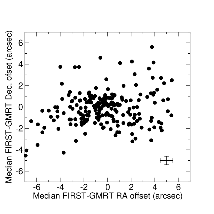
Figure 4: The offsets in RA and declination between $15\sigma$ point sources in the GMRT survey that are detected in the FIRST survey. Each point in the plot is the median offset for all sources in an entire field. The error bars in the bottom right of the Figure show the rms in RA and declination from Fig. 8.

3.4.1 Combining USB+LSB data

We were unable to achieve improved signal-to-noise in images produced by coadding the data from the two GMRT sidebands in the $uv$ plane, so we instead chose to image the USB and LSB data separately and then subsequently co-add the data in the image plane, which always produced output images with improved sensitivity. During the process of co-adding the USB and LSB images, we regridded all of them to a 2 arcsec pixel scale using the aips task regrid, shifted the individual images to remove any systematic position offsets, and smoothed the images to a uniform beam shape across each of the three survey fields.

Fig. 4 shows the distribution of the median offsets between the GMRT and FIRST positions of all $>15\sigma$ point sources in each USB pointing output from the pipeline. The offsets measured for the LSB were always within 0.5 arcsec of the corresponding USB pointing. These offsets were calculated for each pointing using the method described in Section 3.3 as part of the standard pipeline cataloguing routine. As the Figure shows, there was a significant distribution of non-zero positional offsets between our images and the FIRST data, which was usually larger than the scatter in the offsets measured per pointing (shown as an error bar on the bottom right of the figure). It is likely that these offsets are caused by ionospheric phase errors, which will largely be refractive at 325 MHz for the GMRT. Neighbouring images in the survey can have significantly different FIRST-GMRT position offsets, and coadding these during the mosaicing process may result in spurious radio-source structures and flux densities in the final mosaics. Because of this, the measured offsets were all removed using the aips task shift before producing the final coadded USB+LSB images.

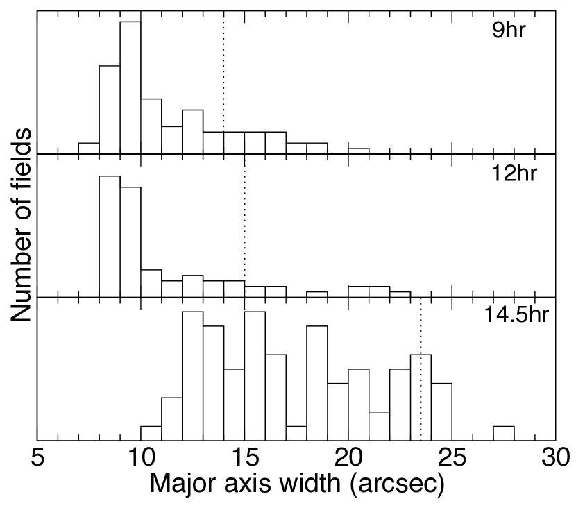
Figure 5: The distribution of the raw clean beam major axis FWHM in each of the three H-ATLAS/GAMA fields from the USB+LSB images output from the imaging pipeline. The dotted line shows the width of the convolving beam used before the mosaicing process. Images with raw clean beam larger than our adopted cutoffs have been discarded from the final dataset.

Next, the USB+LSB images were convolved to the same resolution before they were co-added; the convolution minimises artefacts resulting from different source structures at different resolution, and in any case is required to allow flux densities to be measured from the resulting co-added maps. Fig. 5 shows the distribution in restoring beam major axes in the images output from the GMRT pipeline. The beam minor axis was always better than 12 arcsec in the three surveyed fields. In the 9-h and 12-h fields, the majority of images had better than 10-arcsec resolution. However, roughly 10 per cent of them are significantly worse; this can happen for various reasons but is mainly caused by the poor $uv$ coverage produced by the $2\times 7.5$-minute scans on each pointing. Often, due to scheduling constraints, the scans were observed immediately after one another rather than separated by 6 h which can limit the distribution of visibilities in the $uv$ plane. In addition, when even a few of the longer baselines are flagged due to interference or have problems during their calibration, the resulting image resolution can be degraded.

The distribution of restoring beam major axes in the 14.5-h field is much broader. This is because of the problems with the phase calibrator outlined in Section 2. All visibilities in excess of $20$ k$\lambda$ were removed during calibration of the 14.5-h field and this resulted in degraded image resolution.

The dotted lines in Fig. 5 show the width of the beam used to convolve the images for each of the fields before coadding USB+LSB images. We have used a resolution of 14 arcsec for the 9-h field, 15 arcsec for the 12-h field and 23.5 arcsec for the 14.5-h field. Images with lower resolution than these were discarded from the final data at this stage. Individual USB and LSB images output from the self-calibration step of the pipeline were smoothed to a circular beam using the aips task convl.

After smoothing, regridding and shifting the USB+LSB images, they are combined after being weighted by their indivdual variances, which were computed from the square of the local rms image measured during the cataloguing process. The combined USB+LSB images have all pixels within 30 arcsec of their edge blanked in order to remove any residual edge effect from the regridding, position shifting and smoothing process.

3.4.2 Producing the final mosaics

The combined USB+LSB images were then combined with all neighbouring coadded USB+LSB images within 80 arcmin of their pointing center. This removes the effects at the edges of the individual pointings caused by the primary beam correction and improves image sensitivity in the overlap regions. The final data product consists of one combined mosaic for each original GMRT pointing, and therefore the user should note that there is significant overlap between each mosaic image.

Each combined mosaic image has a width of $100\times 100$ arcmin and 2 arcsec pixels. They were produced from all neighboring images with pointing centers within 80 arcmin. Each of these individual image was then regridded onto the pixels of the output mosaic. The aips task rmsd was run in the same way described during the cataloging (i.e. with a box size of 5 times the major axis of the smoothed beam) on the regridded images to produce local rms noise maps. The noise maps were smoothed with a Gaussian with a FWHM of 3 arcmin to remove any small-scale variation in them. These smoothed noise maps were then used to create variance weight maps (from the sum of the squares of the individual noise maps) which were then in turn multiplied by each regridded input image. Finally, the weighted input images were added together.

The final source catalogue for each pointing was produced as described above from the fully weighted and mosaiced images.

4 Data Products

The primary data products from the GMRT survey are a set of FITS images (one for each GMRT pointing that has not been discarded during the pipeline reduction process) overlapping the H-ATLAS/GAMA fields, the $5\sigma$ source catalogues and a list of the image central positions. This section briefly describes the imaging data and the format of the full catalogues.

4.1 Images

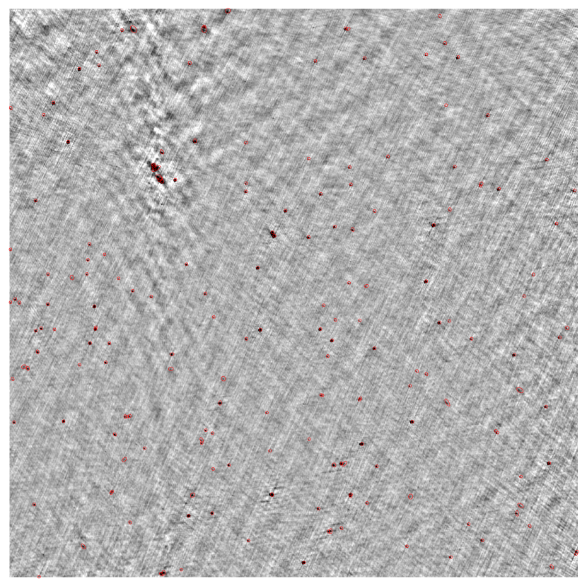
Figure 6: An example $100\times 100$ arcmin² mosaic image from the survey (pointing PNA35 from the 9-h field, centred on RA 08:43:17.6, DEC 00:19:32; see Section 4.2 for a discussion of the field naming scheme) with $5\sigma$ catalogued sources circled in red. Note the reduced dynamic range around the bright (0.9 Jy) double source to the NE.

An example of a uniform mosaic image output from the full pipeline is shown in Fig. 6.

In each field some of the 96 originally observed pointings had to be discarded for various reasons that have been outlined in the previous sections. The full released data set comprises 80 pointings in the 9-h field, 61 pointings in the 12-h field and 71 pointings in the 14.5-h field. In total 76 out of the 288 original pointings were rejected. In roughly 50 per cent of cases they were rejected because of the cutoff in beam size shown in Fig. 5, while in the other 50 per cent of cases the $2\times 7.5$-minute scans of the pointing were completely flagged due to interference or other problems with the GMRT during observing. The full imaging dataset from the survey comprises a set of mosaics like the one pictured in Fig. 6, one for each of the non-rejected pointings.

4.2 Catalogue

Table 3: Ten example lines from the catalogue; full descriptions of each column are in the text.

(1)	(2)	(3)	(4)	(5)	(6)	(7)	(8)	(9)	(10)	(11)	(12)	(13)	(14)	(15)	(16)	(17)	(18)
RA	Dec.	RA	Dec.	$\Delta$RA	$\Delta$Dec.	$A$	${\Delta}A$	$S$	${\Delta}S$	Maj	Min	PA	$\Delta$Maj	$\Delta$Min	PA	Local $\sigma$	Pointing
Degrees (J2000)		$hh$ $mm$ $ss$	$dd$ $mm$ $ss$	arcsec		mJy/bm		mJy		arcsec		∘	arcsec		∘	mJy/bm
130.87617	-00.22886	08 43 30.28	-00 13 43.9	2.5	1.3	6.2	1.1	15.0	3.8	—-	—-	—–	—-	—-	–	1.1	PNA02
130.87746	+02.11494	08 43 30.59	+02 06 53.8	2.3	1.6	12.1	1.3	41.2	5.6	—-	—-	—–	—-	—-	–	1.4	PNA67
130.88025	+00.48630	08 43 31.26	+00 29 10.7	0.5	0.3	129.7	4.7	153.6	6.7	15.9	14.6	13.8	0.5	0.4	9	2.6	PNA51
130.88525	+00.49582	08 43 32.46	+00 29 45.0	0.5	0.4	122.2	4.6	152.1	7.0	—-	—-	—–	—-	—-	–	2.6	PNA51
130.88671	-00.24776	08 43 32.81	-00 14 51.9	0.5	0.3	106.1	3.3	171.3	5.3	21.1	15.0	80.8	0.5	0.4	1	1.0	PNA02
130.88817	-00.89953	08 43 33.16	-00 53 58.3	0.6	0.3	59.6	2.2	118.8	5.0	26.4	14.8	87.5	0.9	0.6	1	1.2	PNA03
130.89171	-00.24660	08 43 34.01	-00 14 47.8	0.5	0.4	34.6	1.5	38.5	2.2	—-	—-	—–	—-	—-	–	1.0	PNA02
130.89279	-00.12352	08 43 34.27	-00 07 24.7	1.2	1.1	4.6	0.8	4.7	1.5	—-	—-	—–	—-	—-	–	0.8	PNA35
130.89971	-00.91813	08 43 35.93	-00 55 05.3	2.4	1.0	7.9	1.5	13.9	3.9	—-	—-	—–	—-	—-	–	1.4	PNA03
130.90150	-00.01532	08 43 36.36	-00 00 55.1	0.9	0.8	6.6	0.8	6.6	1.4	—-	—-	—–	—-	—-	–	0.8	PNA03

Final catalogues were produced from the mosaiced images using the catalogue procedure described in Section 3.3. The catalogues from each mosaic image were then combined into 3 full catalogues covering each of the 9-h, 12-h, and 14.5-h fields. The mosaic images overlap by about 60 per cent in both RA and declination, so duplicate sources in the full list were removed by finding all matches within 15 arcsec of each other and selecting the duplicate source with the lowest local rms ($\sigma_{\rm local}$) from the full catalogue; this ensures that the catalogue is based on the best available image of each source. Removing duplicates reduced the total size of the full catalogue by about 75 per cent due to the amount of overlap between the final mosaics.

The resulting full catalogues contain 5263 sources brighter than the local $5\sigma$ limit. 2628 of these are in the 9-h field, 1620 in the 12-h field and 1015 in the 14.5-h field. Table 3 shows 10 random lines of the output catalogue sorted by RA. A short description of each of the columns of the catalogue follows:

Columns (1) and (2): The J2000 RA and declination of the source in decimal degrees (the examples given in Table 3 have reduced precision for layout reasons).

Columns (3) and (4): The J2000 RA and declination of the source in sexagesimal coordinates.

Columns (5) and (6): The errors in the quoted RA and declination in arcsec. This is calulated from the quadratic sum of the calibration uncertainty, described in Section 5.3, and the fitting uncertainty, calculated using the equations given by Condon (1997).

Columns (7) and (8): The fitted peak brightness in units of mJy beam^-1 and its associated uncertainty, calculated from the quadratic sum of the fitting uncertainty from the equations given by Condon (1997) and the estimated 5 per cent flux calibration uncertainty of the GMRT. The raw brightness measured from the image has been increased by 0.9 mJy beam^-1 to account for the effects of clean bias (see Section 5.2).

Columns (9) and (10): The total flux density of the source in mJy and its uncertainty calculated from equations given by Condon (1997). This equals the fitted peak brightness if the source is unresolved.

Columns (11), (12) and (13): The major axis FWHM (in arcsec), minor axis FWHM (in arcsec) and position angle (in degrees east of north) of the fitted elliptical Gaussian. The position angle is only meaningful for sources that are resolved (i.e. when the fitted Gaussian is larger than the restoring beam for the relevant field). As discussed in Section 5.4, fitted sizes are only quoted for sources that are moderately resolved in their minor axis.

Columns (14), (15) and (16): The fitting uncertanties in the size parameters of the fitted elliptical Gaussian calculated using equations from Condon (1997).

Column (17): The local rms noise ($\sigma_{\rm local}$) in mJy beam^-1 at the source position calculated as described in Section 3.3. The local rms is used to determine the source signal-to-noise ratio, which is used to determine fitting uncertainties.

Column (18): The name of the GMRT mosaic image containing the source. These names consist of the letters PN, a letter A, B or C indicating the 9-, 12- or 14.5-h fields respectively, and a number between 01 and 96 which gives the pointing number within that field (see Fig. 1).

5 Data Quality

The quality of the data over the three fields varies considerably due in part to the different phase and flux calibration sources used for each field, and also due to the variable observing conditions over the different nights’ observing. In particular on each night’s observing, the data taken in the first half of the night seemed to be much more stable than that taken in the second half/early mornings. Some power outages at the telescope contributed to this as well as the variation in the ionosphere, particularly at sunrise. Furthermore, as described in Section 3.4, the poor phase calibrator in the 14.5-h field has resulted in degraded resolution and sensitivity.

5.1 Image noise

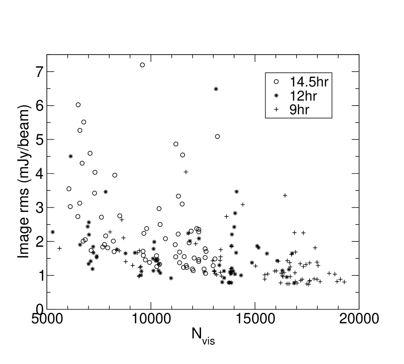
Figure 7: The rms noise measured in the central 1000 pixels of each image plotted against the square root of the number of visibilities. Outliers from the locus are produced by the increased noise in images around sources brighter than 1 Jy.

Fig. 7 shows the distribution of the rms noise measured within a radius of 1000 pixels in the individual GMRT images immediately after the self-calibration stage of the pipeline, plotted against the number of visibilities that have contributed to the final image (this can be seen as a proxy for the effective integration time after flagging). The rms in the individual fields varies from $\sim 1$ mJy beam^-1 in those images with the most visibilities to $\sim 7$ mJy beam^-1 in the worst case, with the expected trend toward higher rms noise with decreasing number of visibilities. The scatter to higher rms from the locus is caused by residual problems in the calibration and the presence of bright sources in the primary beam of the reduced images, which can increase the image noise in their vicinity due to the limited dynamic range of the GMRT observations ($\sim 1000:1$). A bright 7 Jy source in the 12-h field and a 5 Jy source in the 14.5-h field have both contributed to the generally increased rms noise measured from some images. On average, the most visibilities have been flagged from the 14.5-h field because of the restriction we imposed on the $uv$ range of the data. This has also resulted in higher average noise in the 14.5-h fields.

Fig. 2 shows the rms noise maps covering all of the 3 fields. These have been made by averaging the background rms images produced during the cataloguing of the the final mosaiced images and smoothing the final image with a Gaussian with a FWHM of 3 arcmin to remove edge effects between the individual backgound images. The rms in the final survey is significantly lower than that measured from the individual images output from the pipeline self-calibration process, which is a consequence of the large amount of overlap between the individual GMRT pointings in our survey strategy (see Fig. 1). The background rms is $\sim 0.6-0.8$ mJy beam^-1 in the 9-h field, $\sim 0.8-1.0$ mJy beam^-1 in the 12-h field and $\sim 1.5-2.0$ mJy beam^-1 in the 14.5-h field. Gaps in the coverage are caused by having discarded some pointings in the survey due to power outages at the GMRT, due to discarding scans during flagging as described in Section 3.1, and as a result of pointings whose restoring beam was larger than the smoothing width during the mosaicing process (Section 3.4).

5.2 Flux Densities

The $2\times 7.5$-min observations of the GMRT survey sample the $uv$ plane sparsely (see Fig. 3), with long radial arms which cause the dirty beam to have large radial sidelobes. These radial sidelobes can be difficult to clean properly during imaging and clean components which can be subtracted at their position when cleaning close to the noise can cause the average flux density of all point sources in the restored image to be systematically reduced. This “clean bias” is common in “snapshot” radio surveys and for example was found in the FIRST and NVSS surveys (Becker et al., 1995; Condon et al., 1998).

We have checked for the presence of clean bias in the GMRT data by inserting 500 point sources into the calibrated $uv$ data at random positions and the re-imaging the modified data with the same parameters as the original pipeline. We find an average difference between the imaged and input peak flux densities of $\Delta S_{\rm peak}=-0.9$ mJy beam^-1 with no significant difference between the 9hr, 12hr and 14hr fields. A constant offset of $0.9$ mJy beam^-1 has been added to the peak flux densities of all sources in the published catalogues.

As a consistency check for the flux density scale of the survey we can compare the measured flux densities of the phase calibrator source with those listed in Table 2. The phase calibrator is imaged using the standard imaging pipeline and its flux density is measured using sad in aips. The scatter in the measurments of each phase calibrator over the observing period gives a measure of the accuracy of the flux calibration in the survey. In the 9-h field, the average measured flux density of the phase calibrator PHA00 is 9.5 Jy with rms scatter 0.5 Jy; in the 12-h field, the average measured flux density of PHB00 is 6.8 Jy with rms 0.4 Jy; and in the 14.5-h field the average measured flux density of PHC00 is 6.3 Jy with rms 0.5 Jy. This implies that the flux density scale of the survey is accurate to within $\sim 5$ per cent; there is no evidence for any systematic offset in the flux scales.

As there are no other 325-MHz data available for the region covered by the GMRT survey, it is difficult to provide any reliable external measure of the absolute quality of the flux calibration. An additional check is provided by a comparison of the spectral index distribution of sources detected in both our survey and the 1.4-GHz NVSS survey. We discuss this comparison further in Section 7.

5.3 Positions

Table 4: Median and rms of position offsets between the GMRT and FIRST catalogues.

Field	RA offset (arcsec)		Dec. offset (arcsec)
	median	rms	median	rms
9-h	$-0.04$	$0.52$	$0.01$	$0.31$
12-h	$-0.06$	$0.54$	$0.01$	$0.39$
14.5-h	$0.30$	$0.72$	$0.26$	$0.54$

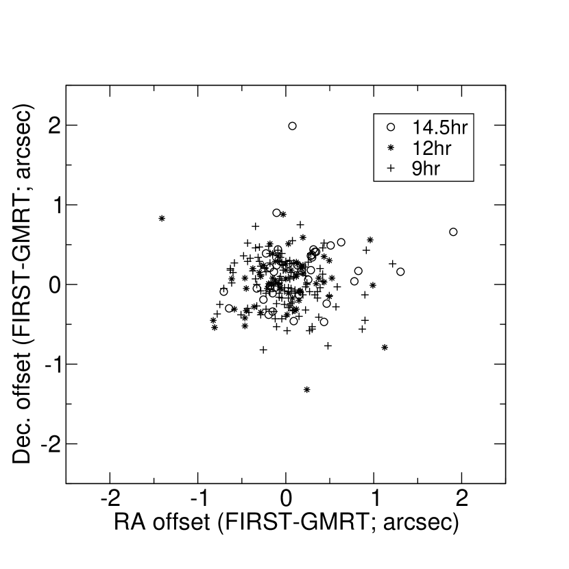
Figure 8: The offsets in RA and declination between $>15\sigma$ point sources from the GMRT survey that are detected in the FIRST survey. The mean offsets in each pointing shown in Fig. 4 have been removed. Different point styles are used to denote the three different H-ATLAS/GAMA fields to show the effect of the variation in the resolution of the GMRT data.

In order to measure the poitional accuracy of the survey, we have compared the postions of $>15\sigma$ GMRT point sources with sources from the FIRST survey. Bright point sources in FIRST are known to have positional accuracy of better than 0.1 arcsec in RA and declination (Becker et al., 1995). We select point sources using the method outlined in Section 3.3. Postions are taken from the final GMRT source catalogue, which have had the shifts described in Section 3.4 removed; the scatter in the measured shifted positions is our means of estimating the calibration accuracy of the positions.

Fig. 8 shows the offsets in RA and declination between the GMRT catalogue and the FIRST survey and Table 4 summarizes the mean offsets and their scatter in the three separate fields. As expected, the mean offset is close to zero in each case, which indicates that the initial image shifts have been correctly applied and that no additional position offsets have appeared in the final mosaicing and cataloguing process. The scatter in the offsets is smallest in the 9-h field and largest in the 14.5-h field, which is due to the increasing size of the restoring beam. The rms of the offsets listed in Table 4 give a measure of the positional calibration uncertainty of the GMRT data; these have been added in quadrature to the fitting error to produce the errors listed in the final catalogues.

5.4 Source Sizes

The strong sidelobes in the dirty beam shown in Fig. 3 extend radially at position angles (PAs) of $40^{\circ}$, $70^{\circ}$ and $140^{\circ}$ and can be as high as 15 per cent of the central peak up to 1 arcmin from it. Improper cleaning of these sidelobes can leave residual radial patterns with a similar structure to the dirty beam in the resulting images. Residual peaks in the dirty beam pattern can also be cleaned (see the discussion of “clean bias” in Section 5.2) and this has the effect of enhancing positive and negative peaks in the dirty beam sidelobes, and leaving an imprint of the dirty beam structure in the cleaned images. This effect, coupled with the alternating pattern of positive and negative peaks in the dirty beam structure (see Fig. 3), causes sources to appear on ridges of positive flux squeezed between two negative valleys. Therefore, when fitting elliptical Gaussians to even moderately strong sources in the survey these can appear spuriously extended in the direction of the ridge and narrow in the direction of the valleys.

These effects are noticeable in our GMRT images (see, for example, Fig. 6) and in the distribution of fitted position angles of sources that appear unresolved in their minor axes (ie. $\phi_{\rm min}-\theta_{\rm min}<\sigma_{\rm min}$; where $\phi_{\rm min}$ is the fitted minor axis size, $\theta_{\rm min}$ is the beam minor axis size and $\sigma_{\rm min}$ is the rms fitting error in the fitted minor axis size) and are moderately resolved in their major axes (ie. $\phi_{\rm maj}-\theta_{\rm maj}>2\sigma_{\rm maj}$; defined by analogy with above) from the catalogue. These PAs are clustered on average at $65^{\circ}$ in the 9-hr field, $140^{\circ}$ in the 12-hr field and at $130^{\circ}$ in the 14.5-hr field, coincident with the PAs of the radial sidelobes in the dirty beam shown in Fig. 3. The fitted PAs of sources that show some resolution in their minor axes (ie. $\phi_{\rm min}-\theta_{\rm min}>\sigma_{\rm min}$) are randomly distributed between $0^{\circ}$ and $180^{\circ}$ as is expected of the radio source population. We therefore only quote fitted source sizes and position angles for sources with $\phi_{\rm min}-\theta_{\rm min}>\sigma_{\rm min}$ in the published catalogue.

6 325-MHz Source Counts

We have made the widest and deepest survey yet carried out at 325 MHz. It is therefore interesting to see if the behaviour of the source counts at this frequency and flux-density limit differ from extrapolations from other frequencies. We measure the source counts from our GMRT observations using both the catalogues and the rms noise map described in Section 5.1, such that the area available to a source of a given flux-density and signal-to-noise ratio is calculated on an individual basis. We did not attempt to merge individual, separate components of double or multiple sources into single sources in generating the source counts. However, we note that such sources are expected to contribute very little to the overall source counts. Fig. 9 shows the source counts from our GMRT survey compared to the source count prediction from the Square Kilometre Array Design Study (SKADS) Semi-Empirical Extragalactic (SEX) Simulated Sky (Wilman et al., 2008, 2010) and the deep 325 MHz survey of the ELAIS-N1 field by Sirothia et al. (2009). Our source counts agree, within the uncertainties, with those measured by Sirothia et al. (2009), given the expected uncertainties associated with cosmic variance over their relatively small field ($\sim 3$ degree²), particularly at the bright end of the source counts.

The simulation provides flux densities down to nJy levels at frequencies of 151 MHz, 610 MHz, 1400 MHz, 4860 MHz and 18 GHz. In order to generate the 325-MHz source counts from this simulation we therefore calculate the power-law spectral index between 151 MHz and 610 MHz and thus determine the 325-MHz flux density. We see that the observed source counts agree very well with the simulated source counts from SKADS, although the observed source counts tend to lie slightly above the simulated curve over the 10-200 mJy flux-density range. This could be a sign that the spectral curvature prescription implemented in the simulation may be reducing the flux density at low radio frequencies in moderate redshift sources, where there are very few constraints. In particular, the SKADS simulations do not contain any steep-spectrum ($\alpha_{325}^{1400}<-0.8$) sources, but there is clear evidence for such sources in the current sample (see the following subsection). A full investigation of this is beyond the scope of the current paper, but future observations with LOFAR should be able to confirm or rebut this explanation: we might expect the SKADS source count predictions for LOFAR to be slightly underestimated.

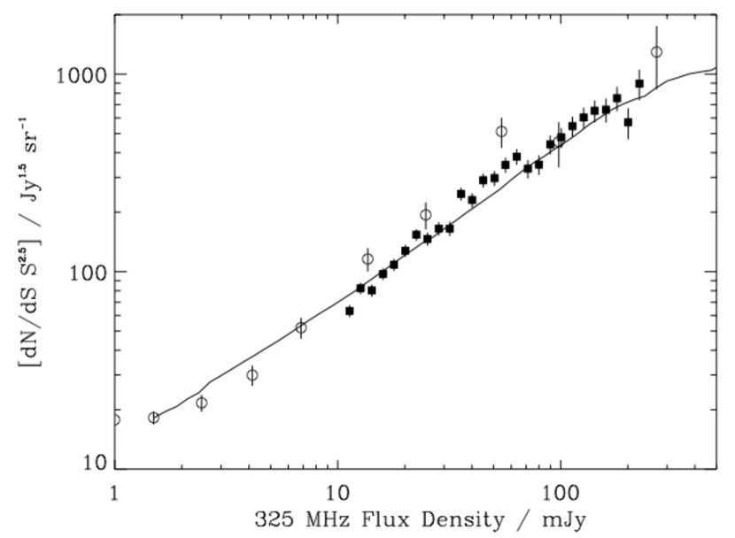
Figure 9: The 325-MHz source counts measured from our GMRT survey (filled squares) and from the survey of the ELAIS-N1 field by Sirothia et al. (2009) (open circles). The solid line shows the predicted source counts from the SKADS simulation (Wilman et al., 2008, 2010).

7 Spectral index distribution

In this section we discuss the spectral index distribution of sources in the survey by comparison with the 1.4-GHz NVSS. We do this both as a check of the flux density scale of our GMRT survey (the flux density scale of the NVSS is known to be better than 2 per cent: Condon et al. 1998) and as an initial investigation into the properties of the faint 325-MHz radio source population.

In all three fields the GMRT data have a smaller beam than the 45 arcsec resolution of the NVSS. We therefore crossmatched the two surveys by taking all NVSS sources in the three H-ATLAS/GAMA fields and summing the flux densities of the catalogued GMRT radio sources that have positions within the area of the catalogued NVSS source (fitted NVSS source sizes are provided in the ‘fitted’ version of the catalogue (Condon et al., 1998)). 3951 NVSS radio sources in the fields had at least one GMRT identification; of these, 3349 (85 per cent) of them had a single GMRT match, and the remainder had multiple GMRT matches. Of the 5263 GMRT radio sources in the survey 4746 (90 per cent) are identified with NVSS radio sources. (Some of the remainder may be spurious sources, but we expect there to be a population of genuine steep-spectrum objects which are seen in our survey but not in NVSS, particularly in the most sensitive areas of the survey, where the catalogue flux limit approaches 3 mJy.)

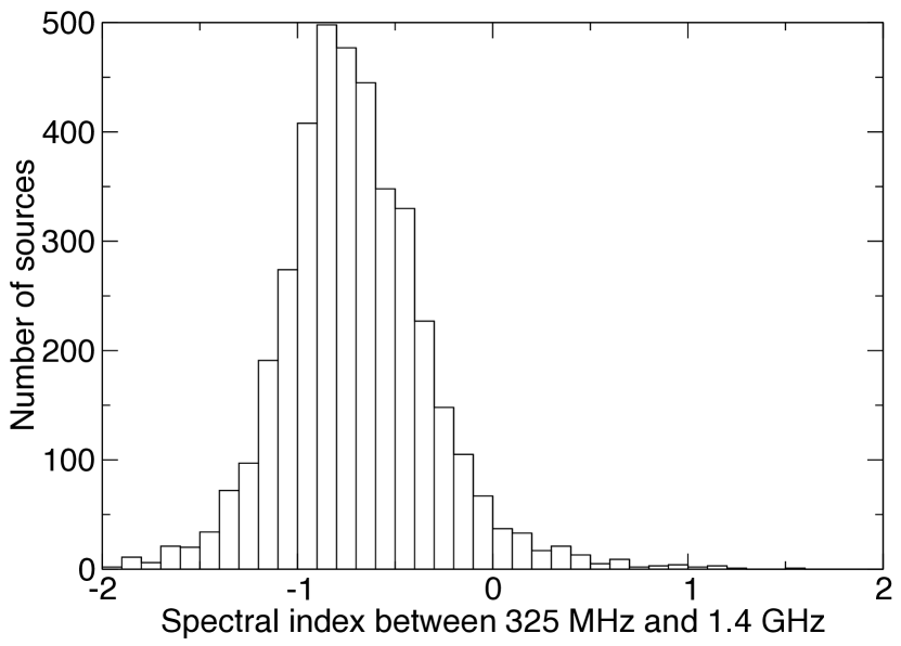
Figure 10: The spectral index distribution between 1.4-GHz sources from the NVSS and 325-MHz GMRT sources.

Fig. 10 shows the measured spectral index distribution ($\alpha$ between 325 MHz and 1.4 GHz) of radio sources from the GMRT survey that are also detected in the NVSS. The distribution has median $\alpha=-0.71$ with an rms scatter of 0.38, which is in good agreement with previously published values of spectral index at frequncies below 1.4 GHz (Mauch et al., 2003; De Breuck et al., 2000; Randall et al., 2012). (Sirothia et al. (2009) find a steeper 325-MHz/1.4-GHz spectral index, with a mean value of 0.83, in their survey of the ELAIS-N1 field, but their low-frequency flux limit is much deeper than ours, so that they probe a different source population, and it is also possible that their use of FIRST rather than NVSS biases their results towards steeper spectral indices.) The rms of the spectral index distributions we obtain increases with decreasing 325-MHz flux density; it increases from 0.36 at $S_{325}>50$ mJy to 0.4 at $S_{325}<15$ mJy. This reflects the increasing uncertainty in flux density for fainter radio sources in both the GMRT and NVSS data.

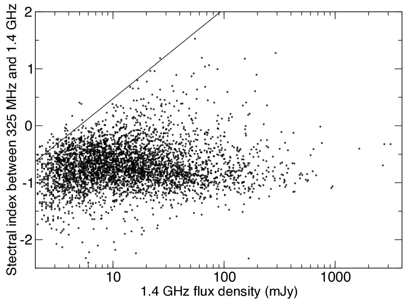
Figure 11: The distribution of the spectral index measured between 325 MHz and 1.4 GHz as a function of 1.4-GHz flux density. The solid line indicates the spectral index traced by the nominal 5 mJy limit of the 325-MHz data.

There has been some discussion about the spectral index distribution of low-frequency radio sources, with some authors detecting a flattening of the spectral index distribution below $S_{1.4}=10$ mJy (Prandoni et al., 2006; Mignano et al., 2008; Owen & Morrison, 2008) and others not (Randall et al., 2012; Ibar et al., 2009). It is well established that the 1.4-GHz radio source population mix changes at around 1 mJy, with classical radio-loud AGN dominating above this flux density and star-forming galaxies and fainter radio-AGN dominating below it (Condon, 1984; Windhorst et al., 1985). In particular, the AGN population below 10 mJy is known to be more flat-spectrum-core dominated (e.g. Nagar et al., 2000) and it is therefore expected that some change in the spectral-index distribution should be evident. Fig. 11 shows the variation in 325-MHz to 1.4-GHz spectral index as a function of 1.4-GHz flux density. Our data show little to no variation in median spectral index below 10 mJy, in agreement with the results of Randall et al. (2012). The distribution shows significant populations of steep ($\alpha<-1.3$) and flat ($\alpha>0$) spectrum radio sources over the entire flux density range, which are potentially interesting populations of radio sources for further study (e.g. in searches for high-$z$ radio galaxies (Miley & De Breuck, 2008) or flat-spectrum quasars).

8 Summary

In this paper we have described a 325-MHz radio survey made with the GMRT covering the 3 equatorial fields centered at 9, 12 and 14.5-h which form part of the sky coverage of Herschel-ATLAS. The data were taken over the period Jan 2009 – Jul 2010 and we have described the pipeline process by which they were flagged, calibrated and imaged.

The final data products comprise 212 images and a source catalogue containing 5263 325-MHz radio sources. These data will be made available via the H-ATLAS (http://www.h-atlas.org/) and GAMA (http://www.gama-survey.org/) online databases. The basic data products are also available at http://gmrt-gama.extragalactic.info/ .

The quality of the data varies significantly over the three surveyed fields. The 9-h field data has 14 arcsec resolution and reaches a depth of better than 1 mJy beam^-1 over most of the survey area, the 12-h field data has 15 arcsec resolution and reaches a depth of $\sim 1$ mJy beam^-1 and the 14.5-h data has 23.5 arcsec resolution and reaches a depth of $\sim 1.5$ mJy beam^-1. Positions in the survey are usually better than 0.75 arcsec for brighter point sources, and the flux scale is believed to be better than 5 per cent.

We show that the source counts are in good agreement with the prediction from the SKADS Simulated Skies (Wilman et al., 2008, 2010) although there is a tendency for the observed source counts to slightly exceed the predicted counts between 10–100 mJy. This could be a result of excessive curvature in the spectra of radio sources implemented within the SKADS simulation.

We have investigated the spectral index distribution of the 325-MHz radio sources by comparison with the 1.4-GHz NVSS survey. We find that the measured spectral index distribution is in broad agreement with previous determinations at frequencies below 1.4 GHz and find no variation of median spectral index as a function of 1.4-GHz flux density.

The data presented in this paper will complement the already extant multi-wavelength data over the H-ATLAS/GAMA regions and will be made publicly available. These data will thus facilitate detailed study of the properties of sub-mm galaxies dectected at sub-GHz radio frequencies in preparation for surveys by LOFAR and, in future, the SKA.

References

- Becker et al. (1995) Becker R. H., White R. L., Helfand D. J., 1995, ApJ, 450, 559
- Colless et al. (2001) Colless M., et al., 2001, MNRAS, 328, 1039
- Condon (1984) Condon J. J., 1984, ApJ, 287, 461
- Condon (1997) Condon J. J., 1997, PASP, 109, 166
- Condon et al. (1998) Condon J. J., Cotton W. D., Greisen E. W., Yin Q. F., Perley R. A., Taylor G. B., Broderick J. J., 1998, AJ, 115, 1693
- De Breuck et al. (2000) De Breuck C., van Breugel W., Röttgering H. J. A., Miley G., 2000, A&AS, 143, 303
- Douglas et al. (1996) Douglas J. N., Bash F. N., Bozyan F. A., Torrence G. W., Wolfe C., 1996, AJ, 111, 1945
- Driver et al. (2011) Driver S. P. et al., 2011, MNRAS, 413, 971
- Eales et al. (2010) Eales S., et al., 2010, PASP, 122, 499
- Griffin et al. (2010) Griffin M. J., et al., 2010, A&A, 518, L3
- Hardcastle et al. (2012) Hardcastle M. J. et al., 2012, MNRAS, in press (arXiv:1211.6440)
- Hardcastle et al. (2010) Hardcastle M. J. et al., 2010, MNRAS, 409, 122
- Ibar et al. (2009) Ibar E., Ivison R. J., Biggs A. D., Lal D. V., Best P. N., Green D. A., 2009, MNRAS, 397, 281
- Jarvis et al. (2010) Jarvis M. J. et al., 2010, MNRAS, 409, 92
- Lawrence et al. (2007) Lawrence A., et al., 2007, MNRAS, 379, 1599
- Mauch et al. (2003) Mauch T., Murphy T., Buttery H. J., Curran J., Hunstead R. W., Piestrzynski B., Robertson J. G., Sadler E. M., 2003, MNRAS, 342, 1117
- Mignano et al. (2008) Mignano A., Prandoni I., Gregorini L., Parma P., de Ruiter H. R., Wieringa M. H., Vettolani G., Ekers R. D., 2008, A&A, 477, 459
- Miley & De Breuck (2008) Miley G., De Breuck C., 2008, A&AR, 15, 67
- Nagar et al. (2000) Nagar N. M., Falcke H., Wilson A. S., Ho L. C., 2000, ApJ, 542, 186
- Owen & Morrison (2008) Owen F. N., Morrison G. E., 2008, AJ, 136, 1889
- Pilbratt et al. (2010) Pilbratt G. L. et al., 2010, A&A, 518, L1
- Poglitsch et al. (2010) Poglitsch A., et al., 2010, A&A, 518, L2
- Prandoni et al. (2006) Prandoni I., Parma P., Wieringa M. H., de Ruiter H. R., Gregorini L., Mignano A., Vettolani G., Ekers R. D., 2006, A&A, 457, 517
- Randall et al. (2012) Randall K. E., Hopkins A. M., Norris R. P., Zinn P.-C., Middelberg E., Mao M. Y., Sharp R. G., 2012, MNRAS, 421, 1644
- Rigby et al. (2011) Rigby E. E. et al., 2011, MNRAS, 415, 2336
- Röttgering et al. (2006) Röttgering H. J. A., et al., 2006, ArXiv Astrophysics e-prints
- Sirothia et al. (2009) Sirothia S. K., Dennefeld M., Saikia D. J., Dole H., Ricquebourg F., Roland J., 2009, MNRAS, 395, 269
- Swarup et al. (1991) Swarup G., Ananthakrishnan S., Kapahi V. K., Rao A. P., Subrahmanya C. R., Kulkarni V. K., 1991, Current Science, 60, 95
- Virdee et al. (2013) Virdee J. S. et al., 2013, MNRAS, 432, 609
- Wilman et al. (2010) Wilman R. J., Jarvis M. J., Mauch T., Rawlings S., Hickey S., 2010, MNRAS, 405, 447
- Wilman et al. (2008) Wilman R. J. et al., 2008, MNRAS, 388, 1335
- Windhorst et al. (1985) Windhorst R. A., Miley G. K., Owen F. N., Kron R. G., Koo D. C., 1985, ApJ, 289, 494
- York et al. (2000) York D. G., et al., 2000, AJ, 120, 1579