Tests of model predictions for the response of stellar spectra and absorption line indices to element abundance variations.

Abstract

To analyse stellar populations in galaxies a widely used method is to apply theoretically derived responses of stellar spectra and line indices to element abundance variations, hereafter referred to as response functions. These are applied in a differential way, to base models, in order to generate spectra or indices with different abundance patterns. In this paper sets of such response functions for three different stellar evolutionary stages are tested with new empirical [Mg/Fe] abundance data for the MILES stellar spectral library. Recent theoretical models and observations are used to investigate the effects of [Fe/H], [Mg/H] and overall [Z/H] on spectra, via ratios of spectra for similar stars. Global effects of changes in abundance patterns are investigated empirically through direct comparisons of similar stars from the MILES library, highlighting the impact of abundance effects in the blue part of the spectrum, particularly for lower temperature stars. It is found that the relative behaviour of iron sensitive line indices are generally well predicted by response functions, whereas Balmer line indices are not. Other indices tend to show large scatter about the predicted mean relations. Implications for element abundance and age studies in stellar populations are discussed and ways forward are suggested to improve the match with behaviours of spectra and line strength indices observed in real stars.

1 Introduction

Element abundance patterns in galaxies hold vital clues to the formation and evolution of their stellar populations. Stellar sources of chemical enrichment contribute different abundance distributions on different timescales. This provides a potential clock for understanding how the integrated stellar population was built up over time and hence the star formation history of a galaxy. The power of this technique relies on our understanding of the different element abundance contributions, quality of the spectroscopic data and on being able to accurately recover representative element abundances in integrated stellar populations from the available data.

Supernova explosions contribute the main sources of chemical enrichments for future generations of stars. SNII explosions enrich the interstellar medium (ISM) in a short timescale ($t\leq 10^{8}$ yrs) with a wide range of heavy elements (including $\alpha$ elements, iron-peak and r-process elements). SNIa explosions enrich the ISM over a much more extended timescale, with mainly iron-peak elements, including prompt ($t\sim 10^{8}$ yrs) and delayed ($t>10^{8}$ to $\sim 10^{10}$ yrs) enrichment (Sullivan et al., 2006; Mannucci, 2008; Maoz, Sharon & Gal-Yam, 2010). Hence the $\alpha$-element to iron ratio is an important indicator of the timescale of star formation. Intermediate mass stars contribute to the lighter elements on relatively long timescale ($t>10^{8}$ to $\sim$few $\times 10^{9}$ yrs). Additional contributions may come from red giant stars and cosmic-ray reactions, however these are not important for the elements considered in the present analysis. Understanding of the relevant element abundance contributions and timescales is still uncertain in some cases. However the match of models to the abundance pattern observed in our own Galaxy (Timmes, Woosley & Weaver, 1995; Tsujimoto et al., 1995; Kobayashi et al., 2006), within a factor of two for most elements up to the iron peak, gives some confidence that these contributions are broadly understood.

Methods of measuring abundance patterns in stellar populations range from colours (e.g. James et al., 2006), which are known to harbour degeneracies (see e.g. Carter et al., 2009; Worthey, 1994) to broad and narrow spectral features (e.g. Rose, 1994; Worthey, 1994; Worthey & Ottaviani, 1997; Serven, Worthey & Briley, 2005; Cenarro et al., 2009). Another, related approach is to use spectral indices from scaled-solar populations to generate proxies for abundance ratios (Vazdekis et al., 2010, , their fig. 25). There are efforts also at generating full integrated spectra (e.g. Coelho et al., 2007; Percival et al., 2009; Lee et al., 2009) and using full spectral fitting (e.g. Walcher et al., 2009) for abundance ratio analysis, however those methods and models are still under development. Information about metallicities, $\alpha$-element to iron ratio and sometimes individual element abundances are recovered from spectral features. One widely used method is to apply element abundance response functions derived from theoretical stellar spectra, which quantify the changes in line-strength indices to variations of individual chemical elements. These response functions are built using theoretical model atmospheres, combined with radiative transfer codes and extensive line lists of atomic and molecular features. These are applied in a differential way, to base models from theoretical or observed spectra with standard abundance patterns, in order to generate spectra or indices for different abundance patterns (e.g. Trager et al., 2000; Thomas et al., 2003; Sansom & Northeast, 2008; Graves & Schiavon, 2008). This can have the advantage of reducing problems associated with absolute line strength predictions from theory, which are limited by incomplete line and molecular band transition information.

Much of the analysis of galaxy abundance ratios in the literature is based on the Lick spectral indices (with band definitions originally from Worthey, 1994; Worthey & Ottaviani, 1997, - hereafter WO97) and response functions for these from theoretical stellar spectra (e.g. Tripicco & Bell (1995); Korn, Maraston & Thomas (2005) - hereafter K05, Houdashelt et al. (2002) - hereafter H02, Tantalo, Chiosi & Piovan (2007); Lee et al. (2009) - hereafter L09). Differential application of theoretical models, to empirical star or simple stellar population (SSP) indices, is currently thought to be one of the best approaches to exploring stellar populations with different abundance patterns (e.g. see discussion in Walcher et al., 2009).

In particular the response functions (R) of K05 are widely applied. Here are some examples. Mendel, Proctor & Forbes (2007) used R from both K05 and H02 to derive ages, metallicities and alpha-element abundances in globular clusters. Schiavon (2007) used R from K05, applied differentially to the empirical stellar library of Jones (1999), in order to generate SSP models with different abundance patterns. These SSPs have since been used in several studies to measure ages and compositions of star clusters and galaxies. Thomas, Johansson & Maraston (2011) used R from K05 to derive ages and abundances of six elements to investigate chemical patterns in globular clusters. Annibali et al. (2011) used R from K05 to derive ages and [$\alpha$/Fe] ratios of dwarf and giant early-type galaxies.

Examples of the use of other response functions in the literature include: Lee, Worthey & Dotter (2009) who used the $\alpha$-enhancement dependencies found in L09, to study the effects of horizontal branch stars and the initial mass function on the integrated light of globular clusters. Serra et al. (2008) used response function from Worthey et al. (private communication), based on the work of L09, to study stellar abundance variations as a function of cold and ionised gas content in a sample of field early-type galaxies.

In this paper we test the robustness of some of those studies listed above that attempt to accurately represent the dependence of spectral line strengths on differing abundance patterns in stars. We do this by testing the response functions, on which those above studies rely, on a star-by-star basis, comparing model predictions to empirical observations of individual stars. This is likely to be one of the cleanest approaches to testing the methods used to measure abundance patterns that are most widely used in the literature. It has the drawback that real star abundance patterns are likely to be more complex than the theoretical models assume, however, it will provide a grounding for the methods used to measure [$\alpha$/Fe].

New empirical data for stars are now available, which these response functions can be tested against in order to check their accuracy against real stars. These data are from the Medium-resolution INT Library of Empirical Spectra (MILES) Sánchez-Blázquez et al. (2006) - hereafter SB06, Cenarro et al. (2007). This spectral library consists of 985 stars covering a wide range of parameter space in effective temperature $T_{\rm eff}$, surface gravity ($g$) and metal abundance (characterised by [Fe/H]). For 752 of these stars the [Mg/Fe] ratio has been compiled in a catalogue (Milone et al., 2011, - hereafter M11). This compilation is based on standardised results from high spectral resolution studies, plus new measurements from the medium resolution MILES stellar library, calibrated to a standard scale using high resolution measurements. In this work we make use of [Mg/Fe] measurements as a proxy for all [$\alpha$/Fe] abundance ratios as a homogeneous nucleosynthetic class and compare differential results from these empirical data with corresponding differential predictions from theoretical models.

This paper is set out as follows. An overview of current knowledge of the effects of differing abundance patterns in stars on their spectral features, published response functions and empirical data used in this paper are discussed in Section 2. Then the response functions are applied and compared to empirical data in Section 3. Effects on spectra due to differing abundance patterns are compared for theoretical and empirical spectra of stars in Section 4. A discussion of the results is given in Section 5 and conclusions are given in Section 6.

2 Effects of Abundance Patterns

2.1 General Considerations

The chemical and physical conditions of a stellar photosphere are imprinted on its emergent spectrum. The major parameter that defines the overall shape of a photospheric spectrum is the effective temperature. Then the abundance pattern, surface convection and surface gravity also affect its spectrum. In particular, we are interested in how the photospheric element abundance pattern affects its emergent spectrum. The overall metallicity [Z/H] can affect the continuum shape as well as absorption line strengths. Iron is the main element being analysed in most spectroscopic studies of stars (especially FGK types) to quantify the chemical abundance in a photosphere. This is because of the existence of a myriad of FeI and FeII lines in the optical range, that are measurable at high resolution and that contribute to spectral line strengths or narrow band indices at lower resolution. The effects of other elements can sometimes be more isolated to particular spectral features, however, to accurately measure these effects it is very important to be clear about what is meant by the metallicity of the star ([Z/H] or [Fe/H]). This is true both for the observations and for the theoretical models used to investigate them.

A simplification assumed in recent years, in order to probe beyond overall metallicity and to uncover the information available in abundance ratios for galaxies, is that all the $\alpha$ elements behave in lock-step. This is a reasonable approximation based on the observational evidence for some $\alpha$ elements from stars in our Galaxy. However, it is not exactly correct (e.g. Bensby et al., 2005; Neves et al., 2009; Franchini et al., 2011). In addition, when handling the metallicity budget in stars, oxygen and carbon are important contributors, whose patterns do not follow the $\alpha$ elements, iron-peak elements or global metallicity, but have their own significant contributions (e.g. McWilliam et al., 2008). For this reason it is more directly linked to observations if models predict behaviours of varying abundance patterns at fixed [Fe/H] (i.e. a single important element) rather than at fixed [Z/H], which is more open to interpretation. Unfortunately this is not always the case and to recover changes at fixed [Fe/H] from these models it is necessary to make assumptions about how [Z/H], [Fe/H] and other abundance indicators such as [$\alpha$/Fe] are related. These uncertainties have been more widely discussed in the literature in recent years (e.g. Schiavon, 2007) and are emphasised here to clarify the difficulties in accurately determining abundance patterns from observed stars or stellar populations, given the currently available models.

2.2 Response Functions in the Literature

Response functions tabulate how much various spectral line strengths alter with element abundance changes in the theoretical model spectra. Application of these response functions allows empirical or theoretical line strengths to be modified for particular abundance patterns, notably enhanced [$\alpha$/Fe] ratios, compared to that of local solar neighbourhood stars. Particular response functions in the literature are:

* Tripicco & Bell (1995) (TB95) - Models for 3 stars: a cool dwarf, a turn-off and a red giant star on a 5 Gyr isochrone. Response functions showed how the Lick indices varied due to a factor of 2 increase in individual elements and in overall metallicity (i.e. from [X/H]=0.0 to [X/H]=+0.3).

* Houdashelt et al. (2002) (H02) - Similar to TB95, but with updated spectral line lists, added H$\gamma$ and H$\delta$ indices and carbon enhancements reduced to +0.15 rather than +0.3 as used for other elements varied in their study (see Worthey 2004 section 3.3). This latter change was an attempt to prevent the C₂ swan bands from becoming unrealistically strong in carbon-rich stars. Their response functions for 3 stars can be obtained from http://astro.wsu.edu/hclee/HTWB02).

* Korn, Maraston & Thomas (2005) (K05) - Similar to TB95, but for a wider range of initial metallicities and star types, with response functions again tabulated for a factor of 2 increase in element abundances from the base models.

* Tantalo, Chiosi & Piovan (2007) (T07) - Generated response functions for a change of $\alpha$ elements from [$\alpha$/H]=0.0 (i.e. solar) to [$\alpha$/H]=+0.4. Individual elements are not varied, but $\alpha$ elements are enhanced as a group. They start from base stars that cover a wider range of atmospheric parameters than in TB95, covering up to 5 values of $T_{\rm eff}$ and 4 values of $\log~{}g$. T07 do not give responses for overall changes in metallicity. These response functions have not yet been widely used subsequently in the literature.

* Lee et al. (2009) (L09)- Expanded the work of H02 and generated response functions for SSPs using many ($\sim 35$) theoretical star spectra at solar metallicity times 10 individual element enhancements (at fixed overall metallicity). Their theoretical spectra are binned to 0.5Å per flux point (however their response functions are not very sensitive to spectral resolution). Plots of some comparisons with K05 for individual theoretical stars are given at http://astro.wsu.edu/hclee/NSSPM$\_$Lick.html; these show similar, but not identical, responses in general between K05 and their evaluations.

Some of the above response functions varied the amounts of individual elements present in the atmospheres, however, they did not always track changes in opacity self consistently. For example, K05 tracked opacity changes for overall metallicity changes ([Z/H]), but treated individual elements like trace elements, whereas the theoretical spectra of L09 were consistently calculated for each abundance pattern. More recent theoretical spectra are available that take into account non-solar abundance patterns plus a more self-consistent approach (e.g. Coelho et al., 2005; Munari et al., 2005). In particular the theoretical stellar spectra of Coelho et al. (2005) are compared to observational spectra in Section 4 of this paper. Response functions for Lick indices are not generally available for these recent theoretical stellar libraries.

Table 1 shows basic characteristics, assumptions and tools used in the generation of published element response functions for stars. This shows the range of different models and assumptions used in generating these response functions.

Table 1: Table showing basic assumptions and tools used in the generation of published element response functions for stars. Elements listed are those tabulated in the response functions. See the Author references in column 1 for details of other references and names given in this table.

Author	Stellar	Spectral	Other	$\alpha$ elements	Other
	Atmosphere	Synthesis	Comments		elements
	Code	Code
H02	MARCS	SSG (Bell & Gustafsson 1989)	Updated TB95	O,Mg,Si,Ca,Ti	C,N,Na,Cr,Fe
K05	MAFAGS	LINFOR	Excludes TiO	O,Mg,Si,Ca,Ti	C,N,Na,Cr,Fe
T07	ATLAS9	Munari et al 2005	Combined $\alpha$	$\alpha$-enhancement	[Z/Z☉]
L09	Plez	FANTOM (Coelho et al. 2005)	Coolest stars	O,Ne,Mg,Si,S,Ca,Ti	C,N,Fe
“	ATLAS	FANTOM (Coelho et al. 2005)	Cool stars
“	MARCS	SSG (Bell et al. 1994)	Medium $T_{\rm eff}$
“	ATLAS	SYNTHE (Kurucz 1970)	Hot stars

2.3 Observations: MILES Lick Line Strength Indices

For the 752 stars for which [Mg/Fe] could be obtained in Milone et al. (2011) we measured line-strength indices in the Lick/IDS system (with the definitions of Trager et al. (1998) and WO97) in the latest version of the MILES stellar spectra (Falcón-Barroso et al., 2011). Errors were estimated from uncertainties caused by photon noise and wavelength calibration (errors in the flux calibration were not taken into account, but the relative flux calibration in the MILES stars have been proved to be very accurate). The line-strength indices were transformed to the Lick system taking into account differences in spectral resolution between the Lick/IDS system and MILES stars following the prescriptions in WO97 (their table 8). The final resolution at which each index was measured is given in Table 2. No further offsets were applied to the measured indices, since both the theoretical response functions and MILES observations were not converted to the Lick/IDS flux system (see K05 section 2.4). Average errors and units for each index are given in the last two columns in Table 2. Appendix A lists all the parameters and Lick indices for MILES stars used in Figs. 1 and 2 of this paper.

Table 2: Lick resolution and MILES average errors. First column gives the index name; second column gives the final spectral resolution (FWHM) at which each index was measured; third column gives the average Lick index errors for the MILES stellar database and their units are given in column 4.

Index	Resolution	Index	Index
	(Å)	Ave. Error	units
H$\delta_{A}$	10.9	0.1895	Å
H$\delta_{F}$	10.9	0.1278	Å
CN1	10.6	0.0050	mag.
CN2	10.6	0.0061	mag.
Ca4227	10.1	0.0850	Å
G4300	9.8	0.1427	Å
H$\gamma_{A}$	9.5	0.1533	Å
H$\gamma_{F}$	9.5	0.0912	Å
Fe4383	9.2	0.1921	Å
Ca4455	9.1	0.0970	Å
Fe4531	9.0	0.1377	Å
C24668	8.8	0.1942	Å
H$\beta$	8.4	0.0740	Å
Fe5015	8.4	0.1528	Å
Mg1	8.4	0.0016	mag.
Mg2	8.4	0.0018	mag.
Mgb	8.4	0.0653	Å
Fe5270	8.4	0.0692	Å
Fe5335	8.4	0.0698	Å
Fe5406	8.4	0.0505	Å
Fe5709	9.2	0.0890	Å
Fe5782	9.2	0.0849	Å
NaD	9.5	0.1103	Å
TiO1	9.7	0.0026	mag.
TiO2	9.7	0.0023	mag.

Table 3: Parameters for base stars that are used for normalisations in the response function tests. The empirical parameters listed are for MILES base stars that match the base stars modelled by K05, within observational errors. These three stars are also modelled by H02. Maximum offsets assumed for this match are: $\Delta$T=$\pm$100K, $\Delta\log~{}g$=$\pm$0.2, $\Delta$[Fe/H]=$\pm$0.1 and $\Delta$[Mg/Fe]=$\pm$0.06. The final column lists reference sources for the model or observation and also indicates the type of data available for [Mg/Fe] determinations for each base star (see M11 for details).

Star	Model or	$T_{\rm eff}$	$\log~{}g$	$[Fe/H]$	$[Mg/Fe]$	Source
Type	Star Name	(K)
CD	K05 table 12	4575	4.60	0.00	0.00	K05 & H02
CD	HD032147	4658	4.47	+0.02	-0.06	M11 (HR)
TO	K05 table 13	6200	4.10	0.00	0.00	K05 & H02
TO	HD016673	6253	4.28	+0.05	+0.05	M11 (HR)
CG	K05 table 14	4255	1.90	0.00	0.00	K05 & H02
CG	HD154733	4200	2.09	0.00	-0.03	M11 (mrBothMg)

3 Testing Response Functions

The original study of TB95 opened the way to differential techniques for tracking abundance ratios. Their work was followed by the more comprehensive study of K05, who included the same theoretical base, solar metallicity stars as TB95, but also explored response functions from lower and higher metallicity base stars. K05 showed that their work agreed well with the results of TB95 and also added results for H$\gamma$ and H$\delta$ indices. Response functions from both these studies have been widely applied in the literature, however we do not test the TB95 response functions here since those of K05 and H02 can be considered as expansions of that earlier work. Theoretical spectra from H02 were revised and expanded on by L09 to form SSPs and their theoretical spectra and SSP response functions are used in the literature, mainly by that group. In this section we test the publicly available star response functions of K05 and H02, which are the ones most widely applied in the literature that we can test. We also test the star response functions used by L09, from information provided by G. Worthey (private communication).

It is important to note that the published tables of response functions tested in this paper tabulate responses of Lick spectral indices to changes in abundance of individual elements, treating individual elements as trace abundances and assuming that the opacity distribution in the atmosphere is not significantly altered by changing the abundance of one element. However, the response function tables (of TB95, K05 and H02) also tabulate changes in indices due to changes in overall metallicity [Z/H] and those values do take into account changes in the structure in the stellar atmospheres due to opacity changes. Since iron is a very important opacity source in stars, and is also most generally the element abundance measured in libraries of stars, we make use of these more self-consistent changes due to [Z/H] to go from theoretical base star indices to stars with different [Z/H]=[Fe/H] values, then we further adjust these index changes to account for non-solar abundance ratios relative to iron, treating the other elements (mostly $\alpha$ elements) as trace element changes. In this way we aim to make best use of the physics that went into the models. For further discussion about the different order in which the response function tables might be applied, see Proctor & Sansom (2002).

3.1 K05 Response Functions

The response functions of K05 were generated from theoretical spectra blurred to the resolution of the Lick/IDS system, according to the resolution variations with wavelength measured by WO97 (see K05 section 2.4). Other corrections to the Lick/IDS standard system were not applied, which is the same approach as for the empirical observations that we are using here. Any remaining differences due to continuum normalisation will be second order effects, mainly affecting the broader band indices. The differential approach used in applying response functions will reduce the need for corrections due to differences in flux calibrations. However, we note that the broader spectral features are the ones most likely to show residual affects due to any remaining flux offsets. These are the CN, Mg and TiO bands.

3.1.1 Solar abundance pattern base models

Although K05 presented response functions for base star models with different metallicities and some different abundance patterns, only those for base stars with solar abundances and solar abundance ratios can be tested here. This is because there are no suitable observed stars in the MILES library to match the specific base star models tabulated in K05 with non-solar abundances. That is, only tables 12-14 (5Gyr models) and tables 15 & 17 (1Gyr models) in K05 have sufficient matching stars in MILES to be able to test them.

The theoretical model values are first derived from K05, using their tables 12, 13 and 14, which give element dependent response functions for a cool dwarf (CD), a turn-off (TO) and a cool giant (CG) star respectively, from a 5 Gyr populations, each of which starts with solar metallicity and abundance ratios. Base star parameters for these three models are shown in Table 3 together with matched observations used to make the normalised comparisons. We apply the response functions twice to the base models; once to generate a set of theoretical indices for the correct [Fe/H] for the star being modelled, by generating indices for a star with that overall [Z/H] (initially with solar abundance ratios), then again to modify those theoretical indices to the correct [$\alpha$/Fe] of each of the observed stars being modelled. We enhance the $\alpha$ elements listed in Table 1, together with Na (see K05, Section 2.1), whilst C, N, Cr and Fe remain un-enhanced. We use this two step process since there are insufficient observed stars of the specific $T_{\rm eff}$, $\log~{}g$, [Fe/H] combinations modelled, which could be used to isolate only [$\alpha$/Fe] enhancement effects.

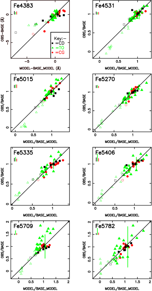
Figure 1: (a). Testing the response functions of K05. Comparison of normalised empirical versus normalised theoretical line strengths for standard Lick indices sensitive to Fe lines in the stellar photospheres. (Note that Fe4531 and Fe5015 are more sensitive to overall metallicity [Z/H] - see K05). The empirical observations are for stars in the MILES spectral library, with known [Fe/H] and [$\alpha$/Fe] (from [Mg/Fe] measurements in M11). Three star types are shown: cool dwarfs (CD, black squares), turn-off stars (TO, green triangles) and cool giants (CG, red circles). The observed stars shown are chosen to all have the same $T_{\rm eff}$ and $\log~{}g$ as the base theoretical star within observational errors, for these three categories. The observed base stars used are HD032147 (CD), HD016673 (TO), HD154733 (CG), which match the atmospheric parameters tabulated for these three star types with solar abundance pattern in K05 (their tables 12, 13 and 14 respectively). Both empirical (vertical) and theoretical (horizontal) axes show either differences (for molecular bands and for lines indices that go negative or close to zero) or ratios (for indices that stay positive for all stars). Average observational errors (2$\sigma$) are attached to the base star points for each index. Systematic errors, estimated from observational uncertainties in base star atmospheric parameters, are indicated by the three vertical lines under the index name on each plot. These are colour coded for each star type modelled. For differences, these systematic error bars represent the maximum vertical offset expected due to combined line-strength uncertainties (added in quadrature), from uncertainties in $T_{\rm eff}$, $\log~{}g$ and [Fe/H]; while for ratios, these error bars indicate the slope uncertainty at one on the vertical axis due to these combined uncertainties. The straight line shows the one-to-one relation in each case. Open symbols show stars with [Fe/H]$<$-0.4, indicating stars with much lower metallicities than the base stars.

The observed stars chosen for the comparison are selected to be those that have the same atmospheric parameters of effective temperature and surface gravity as the tabulated theoretical model stars of K05, within the observational errors on these parameters. For the three base parameters, these errors are $\Delta T$=$\pm 100$ K, $\Delta\log~{}g$=$\pm 0.2$ and $\Delta$[Fe/H]=$\pm 0.1$ dex. For [Mg/Fe] we choose stars within $\Delta$[Mg/Fe]=$\pm 0.06$ dex, since this is the main parameter that we are testing. Only specific base star models have response functions tabulated in K05, therefore that determines our choice of stars that we can test. The observed $T_{\rm eff}$ and $\log~{}g$ values are those given in the MILES spectroscopic database (Cenarro et al., 2007), the observed [Fe/H] and [Mg/Fe] values are those given in M11 and the observed line strengths used are measured from MILES spectra convolved to the same spectral resolution as in K05 (as described in section 2.3 and tabulated in Appendix A). Ratios (or differences) are then formed for both the observations (S) and corresponding theoretical model (M) indices. For a perfect match between observations and response function predictions the ratio M/S would equal 1 (or differences would equal zero).

$$\mathrm{Ratio}=M/S$$ (1)

where:

$$M=\frac{M_{*}([Fe/H],[\alpha/Fe])}{M_{*}(0,0)}$$

is the theoretical model ratio, and

$$S=\frac{S_{*}([Fe/H],[\alpha/Fe])}{S_{*}(0,0)}$$

is the observed star ratio, where the denominators in $M$ and $S$ are the base star values.

Equations used to correct for different abundance patterns using the tabulated responses are from Thomas et al. (2003) (their equation 7) and K05 (their equation 3), for index and flux corrections respectively. The equations used are described below.

Fractional changes in indices ($\Delta I/I_{0}$), due to the combined effects of tabulated response functions $R(i)$ for elements $i$=1 to $n$, from Thomas et al. (2003), their equation 7 are:-

$$\frac{(I_{new}-I_{0})}{I_{0}}=\frac{\Delta I}{I_{0}}=\Pi_{i=1}^{n}(exp[R_{0.3}(i)])^{(\Delta[x_{i}]/0.3)}-1$$ (2)

where $R_{0.3}(i)$ are the tabulated fractional index changes for a factor of 2 increase in abundance of element $i$, and $\Delta[x_{i}]$ is the change in logarithmic abundance of element $i$ (i.e. $\Delta[x_{i}]=+0.3$ for a factor of 2 increase in abundance of element $i$) .

Fractional changes in line fluxes ($\Delta F_{l}/F_{l0}$), due to the combined effects of index changes, from K05, their equation 3 are:-

$$\frac{(F_{lnew}-F_{l0})}{F_{l0}}=\frac{\Delta F_{l}}{F_{l0}}=\Pi_{i=1}^{n}(exp[\frac{\delta F_{l}}{F_{l0}})^{(\Delta[x_{i}]/0.3)}-1$$ (3)

where $\delta F_{l}/F_{l0}$ is the flux change for a factor of 2 increase in abundances of element i.

Index and flux are linked via the equation:-

$$I=W(1-\frac{F_{l}}{F_{c}})$$ (4)

where $F_{c}$ is the continuum flux and $W$ is the bandwidth for index $I$. which leads to:

$$\frac{\delta F_{l}}{F_{l0}}=\frac{\delta I}{(I_{0}-W)}$$ (5)

as in equation 2 of K05, where $R=\delta I/I_{0}$ can be obtained from the tabulated response functions for specific elements and indices. Equation 5 can be used in general to convert from flux changes to index changes.

The corrections to indices are applied for those indices that behave as expected for weak lines (tending to zero strength for the weakest measurements), whereas corrections to fluxes are applied when the defined indices can take positive or negative values. This is to ensure that the property being corrected for element abundance pattern remains positive. After corrections are applied, fluxes are converted back to indices in order to make the comparisons with observations.

Fig. 1(a to e) shows comparison plots for the response functions of K05. The stars plotted in these figures have a wide range in abundance pattern, covering $-2.86<$[Fe/H]$<+0.41$ and $-0.10<$[$\alpha$/Fe]$<+0.53$. Stars with [Fe/H]$<$-0.4 are plotted as open symbols to highlight extrapolations to low metallicity, away from the base star model of [Fe/H]=0.0.

To assess the significance of differences between observations and models, reduced chi-squared values were computed. Some systematic offsets from a one-to-one line in the comparison plots are expected due to slight mismatches between observed and theoretical base star parameters (see Table 3) This is unavoidable, since we have a finite number of observed stars and a finite number of base models for which theoretical response functions are available, and the two do not match perfectly. From the few suitable base stars available, it is found that these systematic offsets are generally small (typically less than twice the average errors on line strengths). They are larger for molecular band features, causing systematic shifts of up to $\pm 0.03$ magnitudes away from the one-to-one lines in the comparison plots. To estimate the size of stystematic offsets expected due to uncertainties in atmospheric parameters of size $\Delta$T=$\pm$100K, $\Delta\log~{}g$=$\pm$0.2 and $\Delta$[Fe/H]=$\pm$0.1, we used the MILES on-line interpolator to generate Lick indices for base stars, varying the parameters by these amounts. The average offsets in one direction are shown in Figure 1, below the index name in each plot. These are shown for each of the three star types tested and represent a maximum typical systematic offset expected due to uncertainties in line strength, added in quadrature, due to uncertainties in all three atmospheric parameters. For comparisons shown as differences, any inaccuracy in base star parameters will appears as a systematic offset above or below the one-to-one line in the comparison plots. For comparisons shown as ratios, any inaccuracy in base star parameter will appear as a systematic fractional difference.

In order to generate error normalisations for evaluating chi-squared, average ($2\sigma$) errors from MILES Lick indices were added in quadrature with mean offsets from the one-to-one line, for each index and each star type. This will account for offsets due to parameter inaccuracies in the base star, but not in the other stars, since the effect of such inaccuracies on Lick indices will be random rather than systematic. The reduced chi-squared ($\chi_{\nu}^{2}$) was found by dividing by the number of stars in each case, since no parameters were being fitted as the comparison is with the one-to-one line prediction.

The results of the comparisons are described in the next section and the derived $\chi_{\nu}^{2}$ values are given in Table 4

3.2 K05 Results

Fig. 1(a) shows the results for Lick indices mainly sensitive to Fe or overall metallicity. These indices show the expected behaviour for observed line-strength changes compared to theoretical ones. There are good one-to-one relations for the differential changes plotted between observations and those derived from theoretical response functions, given the observational errors. The agreement is confirmed by the reduced chi-squared values for these indices, which are typically $\chi_{\nu}^{2}<3$ (see Table 4). Note that conservative 2-sigma error bars are plotted for the random Lick measurement errors, therefore they look larger than the typical data scatter for weak indices such as Fe5782, where this Lick measurement error dominates the scatter. This agreement is not so surprising for features dependent mainly on Fe or overall metallicity, since these dominate spectral changes due to composition changes. Both systematic and random errors are generally larger for TO stars, since metal sensitive line strength are generally weak (and particularly sensitive to temperature uncertainties) in these warmer stars. Other systematic errors are relatively small, consistent with the good one-to-one relations seen in this figure.

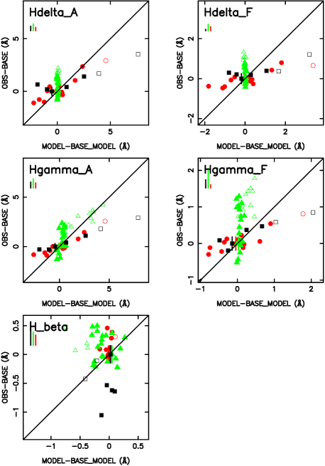
Figure 1: (b). Testing the response functions of K05. Comparison of normalised empirical versus normalised theoretical line strengths for standard Lick indices sensitive to H Balmer lines in the stellar photospheres. Symbols as in Fig. 1(a), with cool dwarfs (CD, black squares), turn-off stars (TO, green triangles) and cool giants (CG, red circles).

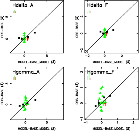
Figure 1: (c). The same as Fig. 1(b) top 4 panels, but for a restricted set of tested stars from MILES, which also have individual C,N and O abundance measurements applied.

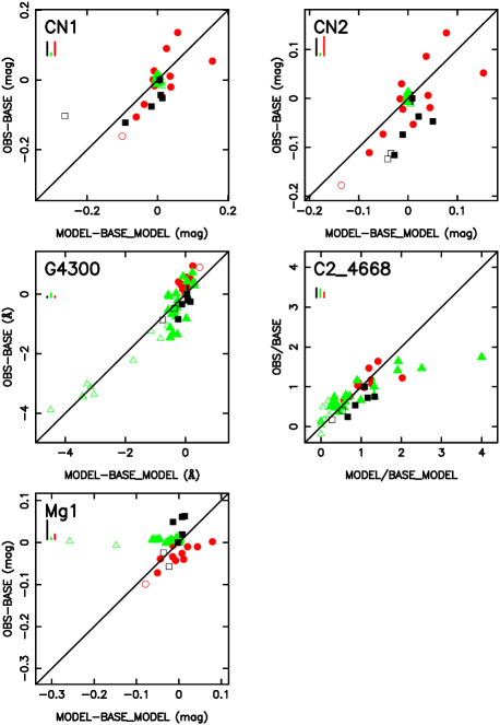
Figure 1: (d). Testing the response functions of K05. Comparison of normalised empirical versus normalised theoretical line strengths for standard Lick indices sensitive to light metal (C,N and O) elements in the stellar photospheres. Symbols as in Fig. 1(a).

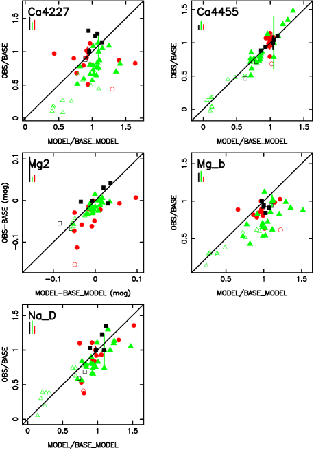
Figure 1: (e). Testing the response functions of K05. Comparison of normalised empirical versus normalised theoretical line strengths for standard Lick indices sensitive to other elements in the stellar photospheres (e.g. Ca4227 is most sensitive to Ca; Ca4455 is weakly sensitive to a variety of elements; Mg₂ and Mgb are most sensitive to Mg; NaD is most sensitive to Na). Symbols as in Fig. 1(a).

Fig. 1(b) shows results for H-Balmer Lick indices. For H$\gamma$ and H$\delta$ the K05 response functions do not mimic well what is happening in real stars as a function of changing abundance patterns ([Fe/H] and [Mg/Fe]). In the CD and CG stars the theoretical response functions predict larger changes than are observed in the empirical star data. For the TO stars, the reverse is true, and the K05 response functions predict negligible variations in these indices as a function of changing abundance patterns (as highlighted, for example in the vertical column of green triangles in the H$\delta_{A}$ plot of Fig. 1(b)). Observed variations of H$\gamma$ and H$\delta$ indices in these warmer stars are larger than the theoretical response functions predict. Some of the vertical scatter in these plots will result from inaccuracies in parameter measurements from star-to-star. Inaccuracies in base star parameters are not the cause of the systematic differences between observations and predictions, since that would cause systematic offsets rather than changes in slope around the mean, as observed in Fig. 1(b). This is confirmed by the relatively small systematic error bars for the cool stars, shown below the index labels on each plot. The differences between observations and predictions are highlighted by the large $\chi_{\nu}^{2}$ values for CG and CD stars, for these higher order Balmer indices (see Table 4).

H$\gamma$ and H$\delta$ indices are known to be affected by CN bands within the definition of these indices. H$\gamma_{A}$ might be sensitive to CH (i.e. G band) affecting its blue pseudocontinuum, whilst CN at 4150Å might affect the red pseudocontinuum. Therefore the difference, in principle, could be due to differences in C and N abundances, with carbon effects being particularly important in the response functions. Linear fits to the cool stars data ([Fe/H]$\geq$-0.4) for H$\gamma$ and H$\delta$ features in Fig. 1(b), give offsets that imply carbon abundance changes much larger than the maximum observed deviations in [C/Fe], which are $<$$\pm$0.4 dex (e.g. Luck & Heiter 2006, 2007). For example, for CG stars in H$\gamma_{A}$ a shift of +1.76Å would bring the lower point onto the 1:1 line, but this requires a change in [C/Fe] of 1.28 dex. Therefore, the slopes for cool stars in Fig. 1(b) cannot be reconciled with the 1:1 line by appealing to systematic changes in carbon abundance alone. Other aspects need to be considered. We searched the literature for individual measurements of C, N or O abundances, relative to Fe, for the stars tested in Fig. 1(b) and found only a few. Fig. 1(c) shows the results of applying these individual abundance measurements. For the cool stars there were only measurements of C and O for 4 CD stars (Luck & Heiter, 2006) and C, N and O for 1 CG star (Luck & Heiter, 2007). Abundances of C, N and O were available for 14 of the TO stars (Takeda & Honda, 2005), which are also plotted. In Fig. 1(c) the response functions from K05 are applied as for Fig. 1(b) except that the columns for responses to individual C, N and O abundances are applied, where available, rather than their assumed links to [$\alpha$/Fe] and [Fe/H] made previously, in Section 3.1.1. The systematic slope difference from the 1:1 line, for 5 cool stars, is still evident in Fig. 1(c), and more measurements on individual C, N and O abundances are needed in future for further tests of the significance of the effects of these individual elements on the higher order Balmer features.

We find in Appendix B that fine tuning the abundance ratios, to take into account mean trends of several elements, makes no significant difference to the mismatch for H$\gamma$ and H$\delta$ indices, using the K05 response functions. This points to overall metallicity response as the cause of the non-unity slopes for cool stars in these four indices (Fig. 1(b)). For H$\beta$ the scatter is larger than expected from observational uncertainties in line strengths, since this index is thought not to be very sensitive to chemistry (e.g. L09, Cervantes & Vazdekis, 2009, based on the synthetic stellar library of Coelho et al. 2005); however, note that a different conclusion for H$\beta$ was reached by Tantalo, Chiosi & Piovan (2007); Cervantes & Vazdekis (2009), based on the synthetic stellar library of Munari et al. (2005). The offsets seen in H$\beta$ can be explained by the systematic error bars plotted, which are particularly large for the CD stars in this index.

Fig.1(d) shows Lick indices that are particularly sensitive to the light metals, C, N and O. These behave qualitatively as expected from the response functions, but with larger scatter than expected from the line-strength measurement errors in most cases. The $\chi_{\nu}^{2}$ values reflect this (see Table 4). The lack of variation in the CN indices in TO stars, predicted from the theoretical response functions, agrees with the observations. For these CN indices in cool stars, errors due to atmospheric parameter uncertainties contribute to the scatter and offsets. Differences in CN band strengths between stars is also likely to contribute to this scatter. The Mg₁ feature, which is most sensitive to carbon, varies far more in the theoretical predictions than in the observations for the TO stars. Mg₁ in these warm TO stars is very weak compared to its values in the CD and CG stars and is observed to vary very little from star-to-star. Therefore its theoretical response function is uncertain. Also, predicted ratios for C₂4668 extend to higher values for some TO stars than in the observations, which do not go above twice the base star line-strengths in these stars. For C₂4668, in TO stars, the response function predictions start to deviate significantly for applications to higher metallicities ([Fe/H]$>$+0.2), where the theoretical predictions have larger line-strengths than the stellar observations, by up to a factor of 2, as seen in the extreme right TO star in Fig.1(d) for the C₂4668 index. However, we note that in luminous elliptical galaxies this index can take higher values (e.g. Zhu, Blanton & Moustakas (2010), their fig. 14). Therefore, except for the weak Mg₁ feature in TO stars and for C₂4668 in TO stars, the response functions are not systematically biased in their predictions for these C,N,O sensitive Lick indices (CN₁, CN₂, G4300, C₂4668 and Mg₁). Future high resolution spectroscopic observations are needed to test the effects of C and N abundance variations on a star-by-star basis.

Fig. 1(e) shows Lick indices sensitive to other elements, including sodium and various $\alpha$ elements (Mg, Ca). Again the response function predictions are approximately followed by the observation, but with large scatter, and some offsets between star types. These systematic offsets shift vertically somewhat when different base stars are used, illustrating the sensitivity of these features to exact photospheric parameters, even within their observational uncertainties. The systematic error bars due to atmospheric parameter uncertainties are relatively large for most of these indices, as seen in this figure. The calcium sensitive index Ca4227 shows large scatter about the one-to-one line, which may also reflect CN contamination effects (Schiavon, 2007) and/or calcium variations that are not fully in step with magnesium variations in the observed stars, since we are using [Mg/Fe] as a proxy for all $\alpha$ elements (O, Ne, Mg, Si, S, Ar, Ca, Ti). In fact there is evidence that calcium does not follow exactly in step with magnesium in a range of environments (e.g. in our Galaxy 0.0$<$[Ca/Fe]$<$[Mg/Fe] for metal-poor stars Franchini et al. (2011) and calcium is even lower [Ca/Fe]$\leq$0.0 for open clusters, Pancino et al. (2010). Also in luminous elliptical galaxies calcium appears to follow iron rather than other $\alpha$ elements such as magnesium (e.g. Vazdekis et al., 1997; Smith et al., 2009, and references therein). In future it may be possible to compile calcium abundances onto a single scale, for a substantial number of MILES stars. Such a [Ca/Fe] catalogue would allow us to test whether differences in [Ca/Mg] are contributing to the scatter for some of the indices. This is particularly important for Ca4227, which currently shows poor agreement between response function predictions and real stars. Ca4455 is weakly sensitive to a number of elements and the observations follow the response function predictions well for this Lick index (see Table 4), with CG stars showing only small variations in both the observations and predictions.

The Mg₂ and Mgb indices, which are sensitive to magnesium, roughly follow the response function predictions, but with quite large scatter and systematic offsets from the one-to-one relation. The variations in Na, sensitive to sodium are qualitatively well predicted by the response functions, for all three star types, but with larger scatter than expected from Lick index uncertainties, for the cool stars.

Table 4: Reduced chi-squared ($\chi_{\nu}^{2}$) values for comparisons of normalised observations (from MILES) versus normalised models (using response functions for [Z/H] and [$\alpha$/Fe] changes in stars). These $\chi_{\nu}^{2}$ values take into account errors added in quadrature from observational errors in Lick indices and systematic offsets due partly to slight base star mismatches. Results are shown for three star types (cool giant = CG, turn-off star = TO, cool dwarf = CD) and for star response functions from Korn et al. 2005 (K05) and Houdasheldt et al. 2002 (H02). The final column shows results comparing normalised observations versus normalised model, using star response functions for [$\alpha$/Fe] changes only, as used in L09 (labelled $\Delta$W12 here), for 71 stars in MILES.

Index	Index	$\chi_{\nu}^{2}$
number	name	———K05———			———H02———			$\Delta$W12 only
		CG	TO	CD	CG	TO	CD	(Any star type)
1	H$\delta_{A}$	4.61	1.75	10.57	17.81	1.76	6.71	5.09
2	H$\delta_{F}$	11.04	1.70	7.01	2.99	1.62	4.06	1.78
3	CN1	7.96	1.02	7.52	8.78	0.61	1.15	14.58
4	CN2	5.61	0.31	1.13	7.75	0.23	1.12	11.14
5	Ca4227	6.45	0.70	2.06	7.79	0.49	4.55	2.64
6	G4300	0.79	2.43	0.67	1.23	2.09	0.68	4.39
7	H$\gamma_{A}$	8.18	3.96	5.88	0.48	2.23	1.40	9.92
8	H$\gamma_{F}$	5.76	1.87	5.61	2.45	1.92	3.36	9.08
9	Fe4383	1.29	3.07	7.05	1.77	1.60	1.51	3.23
10	Ca4455	1.69	0.07	0.42	0.77	0.07	0.30	0.74
11	Fe4531	1.04	0.52	1.53	2.00	0.99	1.61	0.76
12	C24668	25.13	5.75	1.32	26.35	2.45	1.58	6.60
13	H$\beta$	1.12	2.25	1.69	1.66	1.65	1.28	1.32
14	Fe5015	1.19	1.49	1.52	1.14	1.49	6.68	3.02
15	Mg1	2.06	4.80	3.00	1.69	1.12	9.27	16.46
16	Mg2	1.94	1.70	12.07	2.23	1.28	12.69	32.91
17	Mgb	2.73	1.38	1.39	4.04	1.18	1.43	8.16
18	Fe5270	3.61	0.58	2.97	2.38	0.60	1.61	4.66
19	Fe5335	1.47	0.62	4.34	2.38	0.50	4.89	3.54
20	Fe5406	2.09	0.35	3.44	1.90	0.34	2.84	3.24
21	Fe5709	0.47	0.34	0.61	0.42	0.36	0.60	0.52
22	Fe5782	0.87	0.11	0.31	0.75	0.11	0.32	0.52
23	NaD	3.91	0.47	11.32	4.40	0.49	17.85	3.80

The above results do not change significantly if different base stars are used, provided the base stars have the correct atmospheric parameters, within observational errors. This helps to confirm that the trends found are not just a result of small systematic differences in temperature scales between the theoretical and observed stars being compared. For the Mg indices (Mg₁, Mg₂, Mgb) and for Ca4227, in CG stars, differential index changes are slightly more affected by the choice of base star than in most cases. That is, the red circles in Figs. 1 shift significantly, compared to observational index errors, with a change in base star (systematically by $\sim\pm$0.03 mag for Mg₁ and Mg₂, and by $\sim\pm$10% for Mgb and Ca4227). Therefore for these indices it is harder to accurately check the response function predictions with the empirical observations.

A set of response functions for solar abundance models at the younger age of 1 Gyr are given in tables 15 to 17 of K05. Amongst the MILES stars there are base stars that match the CD and CG model stars in these tables (but not for the TO model star). Therefore, comparisons were made of observed versus theoretical normalised indices for these younger CD and CG star models. Results showed similar trends and scatters as previously found for the 5 Gyr models, but with a slight improvement in the H$\delta_{A}$ and H$\gamma_{A}$ indices, for which the normalised observations versus models were closer to one-to-one trends. Scatter for the H$\gamma$ and H$\delta$ features increased in the comparisons for the younger age case.

In summary, most Lick indices follow the predictions of the K05 response functions as well as we can tell from the empirical data, except for H$\gamma_{A}$, H$\gamma_{F}$, H$\delta_{A}$, H$\delta_{F}$ indices, which show systematic deviations from the predictions. These indices lie in the blue part of the spectrum where the flux from cool stars is rapidly changing with wavelength and where the influence of abundance effects is large (see Section 4). Similar results were found for two sets of MILES stars representing ages of 1 and 5 Gyrs respectively. Mg₁ and C₂4668 indices also show systematic deviations from the response function predictions in the case of warm TO stars, as described above.

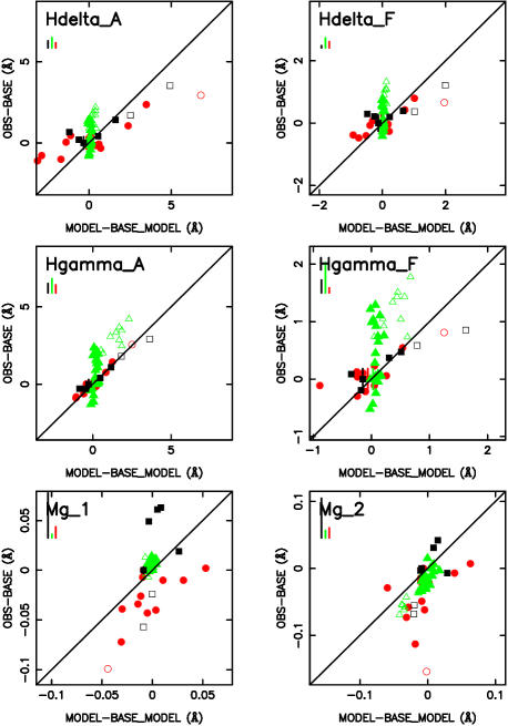
Figure 2: Testing the response functions of H02. Comparison of normalised empirical versus normalised theoretical line strengths for standard Lick indices sensitive to H$\gamma$ and H$\delta$ Balmer lines, showing similar behaviour to that seen in Fig. 1(b); plus Mg₁ and Mg₂ indices. Symbols as in Fig. 1(a).

3.3 H02 Results

An alternative set of models exploring response functions was that of Houdasheldt et al. 2002, who made their response functions for models of 3 stars available at: http://astro.wsu.edu/hclee/HTWB02 (H02). The H02 response functions differ in value from those of K05 and also the line strengths listed at the base abundances are slightly different. Here those tables from H02 are used to test the same 3 stars as in tables 12 to 14 of K05 (in terms of their $T_{\rm eff}$ and $\log~{}g$ parameter and base solar abundances). The same procedure as described in Section 3.1 was applied to test the H02 response functions. Overall the results when comparing to MILES observations are very similar to what is found for the K05 response functions, with some improvements. Fig. 2 shows the H$\gamma$ and H$\delta$ features using H02 response functions, illustrating qualitatively the same problems as with the K05 response functions. We note however, that H$\delta_{F}$, H$\gamma_{A}$ and H$\gamma_{F}$ features for H02 response functions give better agreement with the observations, as seen in Fig. 2 and in Table 4. Therefore the use of H02 might be preferred over K05, particularly for the higher order Balmer indices. H$\beta$ has similar scatter for both K05 and H02 cases. Table 4 also shows that the TO stars are generally better fit by the H02 response functions.

For indices that are treated as positive, but which go slightly negative, the application of response functions becomes invalid. This is seen for Mg₁ in TO stars, for K05 response functions (Fig. 1(d)), and for H$\beta$ in CD and CG stars for H02 response functions. For H02 response functions the Mg₁ index (expressed as a line strength) is positive for all 3 star types, hence TO stars show negligible variation in Mg₁ in the model predictions, in agreement with the observations. Plots for Mg₁ and Mg₂ from H02 are also shown in Fig. 2. The plot for Mg₂ using the H02 response functions looks similar to that in Fig. 1(e) in spread and offsets (also true for Mgb), indicating similar results compared with those of the K05 response functions.

3.4 L09 Results

Lee et al 2009 (L09) note that, in their models, the broader H$\gamma_{A}$ and H$\delta_{A}$ Balmer features are significantly affected by iron abundance. In their on-line comparisons with K05 response functions for individual star models, their plot for H$\delta_{A}$, for example, shows an increase of 2Å (or 5.5Å), for a +0.3 enhancement in [$\alpha$/Fe] at constant [Fe/H]=0.0 (or [Z/H]=0.0); see: http://astro.wsu.edu/hclee/HdA.pdf, red square (or blue square). It is difficult to compare this directly with the spread in observational data for this index, shown in Fig. 1(b), since those data include stars with a range of both [$\alpha$/Fe] and [Fe/H] values, however, the spread in the observations is less than $\sim$ 5Å over a broad range in composition, implying that the L09 models may also overestimate the variation expected in this index.

Although L09 made use of extensions following on from the work of H02, their on-line plots for individual star model response function behaviour indicate different values than those in the H02 tables. Therefore it would be very interesting to be able to test the star response functions of L09. However, L09 did not publish tables of response functions for their 350 model stars (only for their SSPs). Use of the L09 SSP response functions (their table 5) therefore relies on the assumption that they have included different phases of stellar evolution in their correct proportions. It is likely to be better than the use of only 3 stars as is often done in determining response functions for SSPs, however, their published data do not allow us to test the understanding on a star-by-star basis, as we are attempting in this paper.

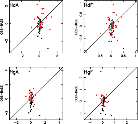
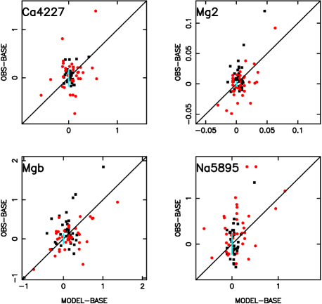
Figure 3: Testing the response functions of W12 for the effects of [$\alpha$/Fe] changes only. Comparison of empirical versus theoretical line-strength differences for standard Lick indices in individual stars. The empirical observations are for stars in the MILES library, with know [Fe/H] and [$\alpha$/Fe] (from [Mg/Fe] measurements in M11). This plot excludes open cluster stars and one star with $|$[Mg/Fe]$|>0.25$. Two star types are shown: cool dwarfs (CD, black squares), and cool giants (CG, red circles), divided at $\log~{}g=3.0$. The observed stars shown are chosen to all have the same $T_{\rm eff}$, $\log~{}g$ and [Fe/H] as the base stars within observational errors. The base stars used are from MILES and have [Mg/Fe]=0.0, within a small tolerance of $\pm$0.01 dex. Average observational errors (2$\sigma$) are attached to one of the star points for each index. The straight line shows the one-to-one relation in each case. Both empirical (vertical) and theoretical (horizontal) axes show differences in Lick indices between observed stars and their matching base stars.

Worthey (priv. comm.- hereafter W12) provided us with model response functions for stars and software used in L09 to generate index changes due to chemistry. These allowed the present authors to generate changes in indices for stars of user defined atmospheric parameters. This information was used to derive three tables equivalent to tables 12 to 14 in K05, for changes due to individual elements in CD, TO and RG stars. For overall metallicity the changes of K05 were assumed, since overall metallicity changes were not available in the W12 star response functions. Using these W12 response functions led to similar results as found using the K05 response functions shown in Fig. 1(a-e), for individual stars. The discrepancies in H$\gamma$ and H$\delta$ indices remained. This similarity of results, using K05 overall metallicity changes with W12 changes to individual elements, supports the fact that overall metallicity is the dominant effect for most indices. That is, we are not finding different results using W12 changes to individual elements.

To probe the effects of [$\alpha$/Fe] changes only, the W12 response functions were used as follows. Stars with [Mg/Fe] close to 0.0 ($\pm$0.01) in MILES were selected, providing 33 base stars. Matching stars in MILES with the same $T_{\rm eff}$, $\log~{}g$, [Fe/H] as these, within errors, but with differing [Mg/Fe] gave 80 matches. Of these, 8 were associated with star clusters and were removed since they were generally lower signal-to-noise. One other star with large [Mg/Fe]=+0.454 was also removed to avoid large changes in metallicity. The remaining stars all had $|$[Mg/Fe]$|<0.25$. This latter restriction is applied here because these W12 response functions do not allow us to track the effects of overall metallicity changes, therefore we can only use them to test trace element changes. Observed index differences for the remaining 71 stars were compared with index differences predicted from W12 models. Fig. 3 shows the results for dwarfs stars (black squares, $\log~{}g\geq 3.0$) and giant stars (red circles, $\log~{}g<3.0$). This shows data points scattering about the one-to-one line for each index, with little sign of any correlations except in the case of magnesium and sodium (Mg₂, Mgb, NaD), for which the correlation coefficients are 0.57, 0.48 and 0.43 respectively. These are significant at $>$99.9% confidence levels, for 71 data points. For these few indices there is evidence that observed indices changes broadly follow indices changes predicted by W12 response functions. The H$\gamma$ and H$\delta$ features show somewhat larger scatter than expected from the typical observational errors (particularly for the giant stars), but no systematic effects are evident that would imply an [$\alpha$/Fe] dependence that is different between the observations and models. Mean offsets are all $<$0.2 dex. Some of the scatter in these differential [$\alpha$/Fe] changes may be due to the fact that the W12 response functions are evaluated from a specified [Fe/H] but keep overall metallicity constant; whereas for the observed stars, their metallicity is characterised by [Fe/H] so we are not exactly comparing like with like, especially at increasingly non-solar [$\alpha$/Fe]. Table 4 shows that the CN, H$\gamma$ and Mg sensitive features agree least within the observational errors for these differential changes. Thus the W12 response functions may be most useful for modelling the effects of element abundance changes, when they can be treated as trace element abundances changes. However, for the current comparisons, this runs into the finite errors on the [Mg/Fe] measurements, therefore weakening this test of the W12 response functions. More accurate measurements of abundances and responses of indices to overall metallicity would be needed to better test the response functions of W12, used in L09.

In summary, these results indicate that the systematic deviations seen in MILES observations relative to K05, for the H$\gamma$ and H$\delta$ features, may result from insufficiently accurate accounting for effects of overall metallicity changes in those response functions. The response functions of H02 agree slightly better with observations for those features. However, they are only available for three model stars. The star response functions of W12 (priv. comm.) provide the widest scope for testing trace element abundance changes but do not allow changes in overall metallicity to be easily tested. Therefore there is as yet no one set of response functions that provide the widest and best fitting to star data. Caution should be exercised particularly in interpreting the H$\gamma$ and H$\delta$ indices in stellar populations, plus indices that reach values close to zero in some stars (H$\beta$, Mg₁) when using response functions.

4 Comparisons of Spectra

Next we go on to test attributes of spectra (rather than indices) to varying abundance patterns.

4.1 Comparison with published model spectra

Cassisi et al. (2004) were the first to compare their theoretical model spectra for enhanced and unenhanced stars. They found the largest differences in the blue part the spectrum, particularly when comparing at constant overall metallicity.

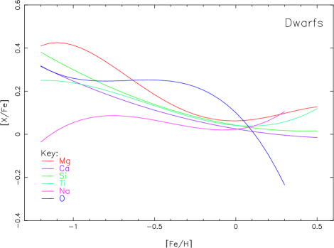
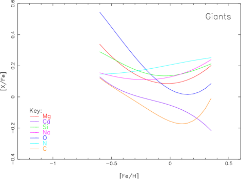
Figure 10: Mean polynomial fits for element abundance ratios [X/Fe] in dwarf stars (left plot) and giants stars (right plot) locally in the disk of the Milky Way. The horizontal ranges plotted illustrate ranges covered by the data (SG05+LH06 for dwarfs and LH07 for giants).

In the current analysis, ratios were created for models of star spectra published by Coelho et al. (2005), for a typical dwarf star ($T_{\rm eff}$=5500K, $\log~{}g=4.0$, [Z/H]=-0.2) and a typical giant star ($T_{\rm eff}$=4500K, $\log~{}g=2.0$, [Z/H]=-0.2) for enhanced ([$\alpha$/Fe]=+0.4) over un-enhanced ([$\alpha$/Fe]=0.0) models, where $\alpha$-elements are considered to be O, Ne, Mg, Si, S, Ca and Ti (see Coelho et al. 2005, section 3.1). The theoretical spectra are published at fixed [Fe/H] values and at these two [$\alpha$/Fe] values. These spectra were interpolated to obtain spectra with overall metallicities at sub-solar abundance [Z/H]=-0.2, using the transformations given by Coelho et al. (2007) (their table 1). This value of overall metallicity was chosen in order to maximize the possibility of finding similar enhanced and unenhanced stars in the observations. Hence the model spectral ratios are compared in Fig. 4 with similar ratios, made from interpolating empirical dwarf star spectra in the MILES library, for particular values of [Fe/H] amd [Mg/Fe]. The interpolator used is an extended version of the 3-dimensional interpolator described in Vazdekis et al. (2003) and Vazdekis et al. (2010) that now allows the user to select stars by [Mg/Fe] (from M11), as a proxy for [$\alpha$/Fe], within the limits imposed by the MILES library coverage of this parameter. This also approximates the link from [Fe/H] to an estimate of overall metallicity [Z/H] by assuming the transformation given by Coelho et al. (2007) (their table 1). Empirical spectra used in Fig. 4 are approximate in enhanced [$\alpha$/Fe] values, due to the limited range of such stars available in the local Solar neighbourhood (as can be seen in fig. 10 of M11).

Qualitatively we see a good agreement between theoretical and empirical spectral ratios plotted in Fig. 4. There are some differences in detail, particularly in the complex spectral region blue-ward of about 4500Å, which are likely to be at least partialy attributed to differences in C, N and O abundances between theoretical models and MILES stars. There are the features modelled by Serven, Worthey & Briley (2005) that affect this region, including CNO3862, CNO4175 as well as the CN bands and features due to other elements. New theoretical spectral models are currently being generated (Coelho - private communication) and a more quantitative comparison will await those models.

Figure 4: Comparison of ratios of spectra with enhanced ([$\alpha$/Fe]=+0.4, [Fe/H]=-0.5) and un-enhanced ([$\alpha$/Fe]=0.0, [Fe/H]=-0.2) abundance patterns, corresponding to fixed overall metallicity ([Z/H]=-0.2) in the models. Enhaced spectra are divided by un-enhanced spectra in each case. The top plot shows dwarf stars ($T_{\rm eff}$=5500K, $\log~{}g=4.0$). The lower plot shows giant stars ($T_{\rm eff}$=4500K, $\log~{}g=2.0$). In each plot: the upper spectral ratio is theoretical, obtained by interpolating theoretical spectra from the library of Coelho et al. 2005 and the lower spectral ratio is observational, obtained by interpolating the MILES empirical spectral library. The theoretical spectral ratios are vertically offset by 1.0 to separate them from the observed spectral ratios shown.

4.2 Comparisons of empirical spectra for specific stars

To qualitatively investigate the influence of $\alpha$-element abundance on empirical stellar spectra, stars were chosen in pairs with similar photospheric parameters in the MILES [Mg/Fe] Catalogue (M11), for a few representative evolutionary stages in the context of SSP modelling. The evolutionary stages analysed are: red normal giant with $T_{\rm eff}$ $\approx$ 4000K and $\log~{}g$ $\approx$ 1.5 (around K5III), main sequence turn-off star with $T_{\rm eff}$ $\approx$ 6600K and $\log~{}g$ $\approx$ 4.2 (around F4V) for an SSP of about 4 Gyr, and a cool main sequence dwarf with $T_{\rm eff}$ $\approx$ 5100K and $log~{}g$ $\approx$ 4.5 (around K1V).

The basic approach was to compute divisions of spectra by choosing pairs of similar stars in terms of $T_{\rm eff}$ and $\log~{}g$ with different abundances, keeping either [Z/H], [Fe/H] or [Mg/H] constant within some level. We assumed the solar abundance pattern from Grevesse & Sauval (1998), as adopted by Coelho et al. (2005). We calculated overall [Z/H] from an abundance pattern, generating values for various combinations of [Fe/H] and [$\alpha$/Fe], assuming all alpha elements are elevated to the same level. Fitting a bi-variable linear function to the results gives the following transformation:

$$[Z/H]=[Fe/H]+0.75(\pm 0.02)[\alpha/Fe]+0.007(\pm 0.006)$$ (6)

valid over the ranges: $-1.5\leq$[Fe/H]$\leq+0.3$ and $-0.2\leq$[$\alpha$/Fe]$\leq+0.6$, and accurate over this range to within $<\pm$0.01 dex ($rms$). This fitted equation gives very similar results to the correspondences tabulated by Coelho et al. (2007), their table 1, which also assumed that all $\alpha$ elements varied in the same way. We used the relation in Equation 6 to search for pairs of stars in MILES [Mg/Fe] catalogue (M11), assuming [$\alpha$/Fe] = [Mg/Fe].

Firstly, assuming [Z/H] constant (but [Fe/H] and [Mg/H] varying), spectra of MILES stars with larger and smaller values of [Mg/H] were divided. Then, considering [Fe/H] unchanged (but [Z/H] and [Mg/H] varying), ratios of spectra of MILES stars were computed, with larger divided by smaller [Mg/H]. To specifically evaluate the influence of [Fe/H] variation on the spectrum as well, ratios of spectra were also obtained by changing [Fe/H] (and [Z/H]) with [Mg/H] constant. The spectrum of a MILES star with larger [Mg/Fe] (and smaller [Fe/H]) was divided by the spectrum of its analogue with smaller [Mg/Fe].

In this approach, any quantitative change in [Mg/H], [Fe/H] or [Z/H] for each comparison needs to be taken into account for a more precise analysis of the results. The differential relationship among the metal abundance parameters is d[Z/H] = d[Fe/H] + 0.75 d[$\alpha$/Fe] , or:

$$d[Z/H]=0.25d[Fe/H]+0.75d[\alpha/H]$$ (7)

in order to express all parameters on a scale relative to hydrogen.

Table 5 presents the set of star pairs adopted for each of the three evolutionary stages considered in the current spectral comparisons. We searched for pairs of similar stars in the MILES [Mg/Fe] Catalogue with differences in $T_{\rm eff}$ and $\log~{}g$ less than or equal to 50K and 0.1 respectively. These fiducial values represent half of one standard deviation of the temperature and gravity errors for FGK stars in the MILES library (Cenarro et al., 2007). A very restrictive condition to fix [Z/H], [Fe/H] or [Mg/H] has also been imposed so that the maximum difference in each metal abundance parameter ($\Delta([X/H])_{max}$ is assumed to be $\leq 0.05$ dex for each pair of stars. Gravity differences had to be somewhat relaxed in order to find some suitable pairs of stars, such that $\Delta\log~{}g\leq 0.2$ for the red giants with fixed [Fe/H]; $\leq 0.5$ for cool dwarfs with [Fe/H] fixed and $\leq 0.3$ for all turn-off stars. The abundance similarities also needed to be relaxed to $\Delta[X/H]\leq 0.07$ for cool dwarfs.

4.2.1 Normal red giant stage

Considering [Z/H] fixed around the solar value, the more magnesium-enhanced red normal giant presents a flux excess in the blue part of spectrum (see Fig. 5a). This excess is a result of the increasing of [Mg/H] and/or decreasing [Fe/H]. When [Fe/H] is assumed constant, with [Z/H] changing below the solar value (Fig. 5b) however, the spectral ratio is relatively flat. By keeping [Mg/H] unchanged close to solar abundance and varying [Fe/H], the spectrum ratio shows that the excess in the blue flux is due to a smaller [Fe/H] (see Fig. 5c). The conclusion is that the blue flux excess for $\alpha$-enhanced red giants in comparison with less $\alpha$-enriched ones at a fixed overall metallicity [Z/H] occurs mainly due to a decrease in [Fe/H] instead of an increase in [$\alpha$/Fe]. However, the level of this effect is somewhat uncertain in the data since the example shown uses an Algol-like system (HD192909). There is some limited capacity to check this result with other pairs of similarly cool red giant stars in MILES. The spectral ratios found vary, but qualitatively show the same results in most cases. Hotter red giant stars show less variation (also see Section 5). This analysis is also limited by the observational errors on all photosperic parameters involved, as qualitatively stressed for temperature and gravity, later in this Section. Therefore we have attempted to concentrate on the most reliable cases.

4.2.2 Main sequence turn-off dwarf for an evolved SSP

Following a similar procedure for three pairs of turn-off stars showed that they vary much less with abundance changes, but still varying most in the blue. Results are shown in Fig. 6, with a smaller vertical scale than used for the red giants in Fig. 5. This smaller variation due to chemistry is not so surprising since these are hotter stars (see Section 5). A few other similar pairs of stars show qualitatively similar behaviour.

4.2.3 Cool main sequence dwarf

Spectral ratios for three pairs of cool dwarf stars are plotted in Fig. 7 with the same vertical scale as for the turn-off stars in Fig. 6. Variations are smaller than for the cool red giant stars, but greater than for the warm turn-off stars. When [Fe/H] is kept fixed (central plot in Fig. 7) there are least variations in the blue. When [Mg/H] is kept fixed (lowest plot in Fig. 7) there are small variations, particularly in the blue, mainly due to changes in [Fe/H]. A few similar examples can be found in the MILES data, qualitatively supporting the relative behaviour shown in Fig. 7.

In future, these spectral ratios will be compared with their exact counterparts in the new theoretical models currently being generated.

Table 5: Set of three pairs of similar MILES stars for a) red giant branch (RGB) stage, b) turn-off (TO) stage and c) cool dwarf (CD) stage. The first two rows in each of these evolutionary categories show the photospheric parameters of a pair of similar stars with fixed [Z/H] around the solar value but varying [Mg/Fe], [Mg/H] and [Fe/H] ($\mid\Delta$([Mg/H])$\mid$ $\geq$ 0.1 dex). The intermediate two rows present the stellar parameters for a pair of similar stars with [Fe/H] fixed around the solar value but changing [Mg/Fe], [Mg/H] and [Z/H] ($\mid\Delta$([Mg/H])$\mid$ $\geq$ 0.25 dex). In the last two rows the parameters of another pair of similar stars is shown with [Mg/H] constant but varying [Mg/Fe], [Fe/H] and [Z/H] ($\mid\Delta$([Fe/H])$\mid$ $\geq$ 0.25 dex). Parameters are from the MILES library, except that [Mg/H], [Mg/Fe], $\sigma$[Mg/Fe] and Notes are from M11, plus [Z/H] is from equation 6. The final column indicates whether [Mg/Fe] is from medium or high resolution spectral studies (see M11 for further details).

#MILES	Type	Name	$T_{\rm eff}$	$\log~{}g$	[Fe/H]	[Mg/Fe]	$\sigma$Mg/Fe	[Mg/H]	[Z/H]	Cat Notes
a) Red Giants			(K)		(dex)	(dex)	(dex)	(dex)	(dex)
[Z/H] constant
0760F	field	HD192909	3880	1.34	-0.43	0.53	0.15	0.10	-0.03	mr Mg5528
0650F	field	HD164058	3902	1.32	-0.05	0.02	0.16	-0.03	-0.03	HR Ae01
[Fe/H] constant
0059F	field	HD009138	4103	1.85	-0.37	0.19	0.10	-0.18	-0.22	mr BothMg
0557F	field	HD137704	4109	1.97	-0.37	-0.16	0.13	-0.53	-0.48	mr Mg5183
[Mg/H] constant
0760F	field	HD192909	3880	1.34	-0.43	0.53	0.15	0.10	-0.03	mr Mg5528
0561F	field	HD139669	3895	1.41	-0.01	0.06	0.15	0.05	0.04	mr Mg5528
b) Turn-off Stars			(K)		(dex)	(dex)	(dex)	(dex)	(dex)
[Z/H] constant
0444F	field	HD109443	6632	4.20	-0.65	0.43	0.10	-0.22	-0.32	mr BothMg
0525F	field	HD130817	6585	4.08	-0.46	0.14	0.10	-0.32	-0.35	mr BothMg
[Fe/H] constant
0482F	field	HD119288	6594	4.03	-0.46	0.53	0.10	0.07	-0.06	mr BothMg
0412F	field	HD099747	6604	4.06	-0.51	0.16	0.10	-0.35	-0.38	mr BothMg
[Mg/H] constant
0444F	field	HD109443	6632	4.20	-0.65	0.43	0.10	-0.22	-0.32	mr BothMg
0504F	field	HD125451	6669	4.44	0.05	-0.22	0.10	-0.17	-0.11	mr BothMg
c) Cool Dwarfs			(K)		(dex)	(dex)	(dex)	(dex)	(dex)
[Z/H] constant
0145F	field	HD026965	5073	4.19	-0.31	0.34	0.12	0.03	-0.05	HR T98LH05
0684F	field	HD171999	5031	4.65	-0.10	-0.03	0.15	-0.13	-0.12	mr Mg5528
[Fe/H] constant
0529F	field	HD132142	5108	4.50	-0.55	0.34	0.05	-0.21	-0.29	HR BM05
0138F	field	HD025673	5150	4.50	-0.60	0.07	0.05	-0.53	-0.54	HR BM05
[Mg/H] constant
0750F	field	HD190404	5051	4.45	-0.17	0.39	0.05	0.22	0.13	HR BM05
0322F	field	HD075732	5079	4.48	0.16	0.09	0.05	0.25	0.23	HR BM05

Figure 5: Ratios of pairs of MILES spectra a) of a pair of analogue stars for the RGB stage, fixing [Z/H] around the solar value but varying [Mg/H] and [Fe/H] ($\Delta$([Mg/H]) = +0.13 and $\Delta$([Fe/H]) = -0.38 dex). b) of a pair of analogue stars for the RGB stage, keeping [Fe/H] fixed slightly below the solar value but changing [Mg/H] and [Z/H] ($\Delta$([Mg/H]) = +0.35 and $\Delta$([Z/H]) = +0.26 dex). c) of a pair of analogue stars for the RGB stage, assuming [Mg/H] constant but varying [Fe/H] and [Z/H] ($\Delta$([Fe/H]) = -0.42 and $\Delta$([Z/H]) = -0.07 dex). The star names and their parameters are listed in Table 5.

Figure 6: Ratios of pairs of MILES spectra a) of a pair of analogue stars for the TO stage, fixing [Z/H] below the solar value but varying [Mg/H] and [Fe/H] ($\Delta$([Mg/H]) = +0.10 and $\Delta$([Fe/H]) = -0.19 dex). b) of a pair of analogue stars for the TO stage, keeping [Fe/H] fixed below the solar value but changing [Mg/H] and [Z/H] ($\Delta$([Mg/H]) = +0.42 and $\Delta$([Z/H]) = +0.44 dex). c) of a pair of analogue stars for the TO stage, assuming [Mg/H] constant but varying [Fe/H] and [Z/H] ($\Delta$([Fe/H]) = -0.70 and $\Delta$([Z/H]) = -0.21 dex). The star names and their parameters are listed in Table 5.

Figure 7: Ratios of pairs of MILES spectra a) of a pair of analogue stars for the CD stage, fixing [Z/H] around the solar value but varying [Mg/H] and [Fe/H] ($\Delta$([Mg/H]) = +0.16 and $\Delta$([Fe/H]) = -0.21 dex). b) of a pair of analogue stars for the CD stage, keeping [Fe/H] fixed below the solar value but changing [Mg/Fe] and [Z/H] ($\Delta$([Mg/H]) = +0.32 and $\Delta$([Z/H]) = +0.25 dex). c) of a pair of analogue stars for the CD stage, assuming [Mg/H] constant but varying [Fe/H] and [Z/H] ($\Delta$([Fe/H]) = -0.33 and $\Delta$([Z/H]) = -0.10 dex). The star names and their parameters are listed in Table 5.

4.2.4 Effect of parameter errors on spectrum ratios

We investigated the impact of errors in $T_{\rm eff}$ and $\log~{}g$ on flux ratios of similar stars. In the MILES database the typical uncertainty for FGK stars is 100K in temperature and 0.2 in $\log~{}g$. To analyse the influence of significant temperature and surface gravity deviations we computed spectrum ratios for selected pairs of analogue stars with very similar parameters except for temperature (which deviated by $\geq 275$K) or log gravity (which deviated by $\geq 0.6$).

For cool giants a temperature increase of more than 3 times the temperature uncertainty produces more blue flux (from 20% upwards) and residuals in lines across the spectrum, appearing all as excesses or deficiencies in the spectrum ratios. The difference dominates in the blue, however, the whole spectrum is affected to some extent. Flux ratios analysed for pairs of RGB stars do not exhibit this pattern due to such $T_{\rm eff}$ deviations. Also the pattern of effects produced by $\log~{}g$ uncertainties are not seen in the RGB flux ratios shown in Fig. 5. For the TO stars, effects of these temperature and gravity uncertainties are not significant, except that Ca II H-K lines just below 4000 Å are affected by changes in both $\log~{}g$ and $T_{\rm eff}$ at some level (perhaps affecting the spectrum ratios shown in Fig. 6, especially Fig. 6c which shows the constant [Mg/H] case). The impact of temperature uncertainties on the CD spectrum ratios exhibits qualitatively similar behaviour as in the RGB case, but with a smaller magnitude since the CD stars are somewhat hotter. There is no significant effect of gravity uncertainty on flux ratios for the CD case, except for the constant [Fe/H] case, where the spectrum ratio is close to one throughout (Fig. 7b). Therefore we are confident that the differences that we are seeing in Figs. 5, 6 and 7 are not dominated by $T_{\rm eff}$ and $\log~{}g$ parameter uncertainties in these MILES similar star pairs.

4.2.5 Influence of C, N and O abundances on [Z/H] estimation

The CNO group is an important contributor to the total metal content and integrated opacity in a stellar phostosphere. To investigate the impact of individual abundances of carbon, nitrogen and oxygen on the global metallicity estimate, we recomputed [Z/H] on a star-by-star basis (for the stars listed in Table 5) adopting their published abundances where available. When either there is no elemental abundance available or the star’s collected [Fe/H] does not match its MILES value (within 2$\sigma[Fe/H]$=0.2 dex), we estimated [X/Fe] from observed mean galactic trends for local disk stars. Table 6 compiles the individual re-estimated [Z/H] as well as the CNO abundances. This approach should be more precise than the previously applied approximation (Eq. 6), in which the $\alpha$-element abundances (including oxygen) are all represented by magnesium, with carbon and nitrogen assumed to be scaled-solar. The galactic trends of [C/Fe] and [N/Fe] as a function of [Fe/H] for dwarf stars are those from Takeda & Honda (2005), i.e. [C/Fe] = -0.21($\pm$0.03)[Fe/H] + 0.014($\pm$0.006), and [N/Fe] around the solar value (obtained from a sample of 160 nearby FGK dwarfs/subgiants with -0.7 $\leq$ [Fe/H] $\leq$ +0.4). The trends of [O/Fe] for dwarfs and [C,N,O/Fe] for giants are listed in Appendix B (Table B1) and illustrated in Fig. B1; they are respectively from Soubiran & Girardi (2005) and Luck & Heiter (2007).

According to our simpler procedure to estimate [Z/H], the variation in [Z/H] is linearly correlated to the variations in [Fe/H] and [$\alpha$/H] (Eq. 7). To evaluate how the individual CNO abundances modify this approximation, we checked if $\Delta$[Z/H], $\Delta$[Fe/H] and $\Delta$[$\alpha$/H] (Mg or O as a proxy) follow this differential relationship considering typical abundance errors (about 0.1 dex on average). In summary our main results are as follows for the pairs of similar stars given in Table 5 and the differences in estimated [Z/H] values are plotted in Fig. 8.

• ] constant: $\Delta$[Fe/H], accounting for the small variations in [Z/H] (of 0.08 and 0.13 dex in the RG and TO stars respectively), is better correlated with $\Delta$[O/H] instead of $\Delta$[Mg/H]. For the CD case, the variation in [Z/H] is very close to zero.

• ] constant: The expected correlation $d[Z/H]=0.75d[\alpha/H]$ from Eq. 7 works (within the abundance uncertainties), except that the two RG stars show the largest deviations, as seen plotted in Fig. 8.

• ] constant: The variation in [Fe/H] correlates well with $\Delta$[Z/H] following our simple approximation in Eq. 7. For the TO case, the relation would be better reproduced if [$\alpha$/H] differences, in elements other than Mg, were allowed for. In the CD case, the differential relationship (Eq. 7) would be acceptable if the outlying data from Zhao et al. (2002) were excluded (see their [O/H] value in Table 6).

In general we find that the few available C, N & O individual abundances have some influence on the estimation of overall metallicity [Z/H], but that it is not a significant affect, taking into account the abundance uncertainties (there are only two stars that deviate from Eq. 7 by 2 to 3$\sigma[Fe/H]$, both from the [Fe/H] constant case of RG stars, where [O/H] does not follow [Mg/H] - see Fig. 8). Only one stellar spectral comparison is probably invalid (the [$\alpha$/H] constant case of TO stars). Thus our standard approach expressed by Eqs. 6 & 7 can be considered as a reliable approximation of [Z/H] for the present analysis. However adopting well-determinate CNO abundances in a homogeneous system will provide more precise global metallicity estimates in future. We will be able to redo the spectral-ratio analysis when we have completed an abundance compilation for as many MILES stars as possible. An important aspect of this task will be to transform all [X/Fe] onto a uniform system, checking the scales of T_eff, $\log$ g and [Fe/H] of each referenced work against the MILES parameters system. This is a longer-term project that is currently in progress.

Figure 8: Histogram of differences between [Z/H]new (derived using individual C, N, O, Mg and Fe abundances from Table 6) and [Z/H] estimated using Eq. 6.

Table 6: C, N and O data for pairs of similar stars (corresponding to those in Table 5).

Name	$[{{\rm Fe}\over{\rm H}}]$	$[{{\rm Mg}\over{\rm Fe}}]$	$[{{\rm Mg}\over{\rm H}}]$	$[{{\rm Fe}\over{\rm H}}]$	$[{{\rm C}\over{\rm Fe}}]$	$[{{\rm C}\over{\rm H}}]$	Ref	$[{{\rm N}\over{\rm Fe}}]$	$[{{\rm N}\over{\rm H}}]$	Ref	$[{{\rm O}\over{\rm Fe}}]$	$[{{\rm O}\over{\rm H}}]$	Ref	Notes	$[{{\rm Z}\over{\rm H}}]$
	———MILES———						or			or			or		new
							Trend			Trend			Trend
	dex	dex	dex	dex	dex	dex		dex	dex		dex	dex			dex
=RED GIANTS=
[Z/H] constant
HD192909	-0.43	0.53	0.10		0.03	-0.40	Trend	0.15	-0.28	Trend	0.38	-0.05	Trend		-0.10
HD164058	-0.05	0.02	-0.03		-0.14	-0.19	Trend	0.20	0.15	Trend	0.07	0.02	Trend		-0.02
[Fe/H] constant
HD009138	-0.37	0.19	-0.18	-0.34	0.19	-0.15	LH07	0.15	-0.19	LH07	0.52	0.18	LH07	CNO	0.01
HD137704	-0.37	-0.16	-0.53		0.01	-0.36	Trend	0.16	-0.21	Trend	0.32	-0.05	Trend		-0.19
[Mg/H] constant
HD192909	-0.43	0.53	0.10		0.03	-0.40	Trend	0.15	-0.28	Trend	0.38	-0.05	Trend		-0.10
HD139669	-0.01	0.06	0.05		-0.15	-0.16	Trend	0.20	0.19	Trend	0.05	0.04	Trend		0.01
=TO STARS=
[Z/H] constant
HD109443	-0.65	0.43	-0.22		0.15	-0.50	Trend	0.00	-0.65	Trend	0.25	-0.40	Trend		-0.40
HD130817	-0.46	0.14	-0.32		0.11	-0.35	Trend	0.00	-0.46	Trend	0.26	-0.20	GL93	O	-0.27
[Fe/H] constant
HD119288	-0.46	0.53	0.07		0.11	-0.35	Trend	0.00	-0.46	Trend	0.25	-0.21	Trend	*	-0.19
HD099747	-0.51	0.16	-0.35		0.12	-0.39	Trend	0.00	-0.51	Trend	0.25	-0.26	Trend		-0.32
[Mg/H] constant
HD109443	-0.65	0.43	-0.22		0.15	-0.50	Trend	0.00	-0.65	Trend	0.25	-0.40	Trend		-0.40
HD125451	0.05	-0.22	-0.17		0.00	0.05	Trend	0.00	0.05	Trend	-0.19	-0.14	GL93	O	-0.07
=COOL DWARFS=
[Z/H] constant
HD026965	-0.31	0.34	0.03	-0.24	0.14	-0.10	LH06	0.00	-0.31	Trend	0.12	-0.12	LH06	CO	-0.15
				-0.28	0.08	-0.23	Trend	0.00	-0.31	Trend	0.38	0.10	PM11	O	-0.02
				-0.31	0.08	-0.23	Trend	0.00	-0.31	Trend	0.41	0.10	Re07	O	0.00
				-0.31	0.42	0.11	Ee04	0.00	-0.31	Trend	0.23	-0.08	Trend	C	-0.02
HD171999	-0.10	-0.03	-0.13		0.03	-0.07	Trend	0.00	-0.10	Trend	0.16	0.06	Trend	**	-0.01
[Fe/H] constant
HD132142	-0.55	0.34	-0.21	-0.54	0.13	-0.42	Trend	0.00	-0.55	Trend	0.24	-0.30	Ce06	$\alpha$	-0.33
				-0.45	0.13	-0.42	Trend	0.00	-0.55	Trend	0.51	0.06	PM11	O	-0.17
					0.13	-0.42	Trend	0.00	-0.55	Trend	0.25	-0.30	Trend		-0.33
HD025673	-0.60	0.07	-0.53	-0.53	0.14	-0.46	Trend	0.00	-0.60	Trend	0.15	-0.38	Ce06	$\alpha$	-0.48
				-0.50	0.32	-0.18	DM10	0.00	-0.60	Trend	0.15	-0.35	DM10	CO	-0.42
					0.14	-0.46	Trend	0.00	-0.60	Trend	0.25	-0.35	Trend		-0.42
[Mg/H] constant
HD190404	-0.17	0.39	0.22		0.05	-0.12	Trend	0.00	-0.17	Trend	0.19	0.02	Trend		0.02
HD075732	0.16	0.09	0.25	0.32	-0.02	0.14	Trend	0.00	0.16	Trend	0.04	0.36	Ze02	O	0.19
				0.31	-0.02	0.14	Trend	0.00	0.16	Trend	-0.18	0.13	PM11	O	0.09
				0.33	-0.02	0.14	Trend	0.32	0.65	Ee04	-0.05	0.11	Trend	N	0.18
				0.33	-0.02	0.14	Trend	0.00	0.16	Trend	-0.20	0.13	Ee06	O	0.09
					-0.02	0.14	Trend	0.00	0.16	Trend	-0.05	0.11	Trend		0.15

ADDITIONAL NOTES FOR TABLE 6. Reference: LH07=Luck & Heiter 2007; GL93=Garcia Lopez et al. 1993; LH06=Luck & Heiter 2006; PM11=Petigura & Marcy 2011; Re07=Ramírez et al. 2007; Ee04=Ecuvillon et al. 2004; Ce06=Casagrande et al. 2006; DM10=Delgado Mena et al. 2010; Ze02=Zhao et al. (2002); Ee06=Ecuvillon et al. (2006).

(i) For galactic trend estimates only: [X/H] = [Fe/H]_MILES + [X/Fe]_Trend; otherwise [X/H] = [Fe/H]_Ref + [X/Fe]_Ref.

(ii) Mean galactic trends of [X/Fe] as a function of [Fe/H] for local disk stars: Giants C & N: Takeda & Honda (2005); O: Soubirane & Girard (2005) Dwarfs C, N and O: LH07

(iii) * 1 work, [Fe/H] deviates from MILES (HD119288): Clementini et al. (1999)

(iv) ** 2 works, [Fe/H] deviates from MILES (HD171999): PM11, and Trevisan et al. (2011)

5 Discussion

Uncertainties in response functions may lead to different predictions for stellar population ages as well as abundances. For example, for a CG star, an increase in [$\alpha$/Fe] of +0.3 at fixed [Fe/H]=0.0 leads to predicted changes in H$\delta_{F}$ of +0.56Å (from K05 response functions) and +0.36Å (from H02 response functions), a difference in predictions of $\Delta$H$\delta_{F}$=+0.20Å. Alternatively, using response functions for overall [Z/H] then lowering the Fe-peak elements and Carbon back down to solar leads to predicted changes in H$\delta_{F}$ of -0.08Å (from K05 response functions) and +0.32Å (from H02 response functions). The difference between these predictions is thus $\Delta$H$\delta_{F}$=+0.40Å. This is significant when compared with changes in H$\delta_{F}$ expected with age in SSPs (at 5 Gyr, [Fe/H]=0.0), as shown in Schiavon (2007), their fig. 7: age increases by $\sim$3 Gyr for a drop of 0.4Å in H$\delta_{F}$. Thus the larger predicted increase in H$\delta_{F}$ from K05 response functions would result in a slightly older age estimate, since more of the H$\delta_{F}$ increase is explained away as due to abundance ratio effects in this case.

This effect is diluted when a range of stellar types is considered in the calculations. Following the luminosity weighting combination used by Trager et al. (2000) (53, 44 and 3% of the light from CG, TO and CD stars respectively, approximating a 5 Gyr population), we raise only the $\alpha$-element group by +0.3 in the log and find a difference of $\Delta$H$\delta_{F}$=+0.07Å, between K05 and H02 response function predictions. This corresponds to a change in age of less than 1 Gyr. Larger differences between K05 and H02 predictions are found when the [Z/H] column of the response functions is used (as discussed in Section 3 above), which can lead to significant age uncertainties for an SSP.

Deviations for the higher order Balmer features in cool stars, seen in Fig. 1(b), correlate more strongly with the metallicity of the stars (characterised by [Fe/H]) than they do with [Mg/Fe]. We used the column for overall [Z/H] changes in the response functions tested in Figures 1 & 2, in order to reach the correct [Fe/H] values (for solar abundance ratios), before modifying the index changes due to non-solar abundance ratios using the $\alpha$-element columns of the response function tables. Therefore, it is likely that the most uncertain response function predictions for these features in K05 are the ones tabulated for [Z/H] changes. More accurate theoretical predictions for these changes are needed in the blue part of the spectrum in order to make accurate predictions for how H$\gamma$ and H$\delta$ absorption features should vary with overall metallicity and with [Fe/H].

Another area of uncertainty is how individual elements may vary on a star-to-star basis and the effect that this may have on the current comparisons. To address this question more accurately, it will be important in future work to obtain high spectral resolution observations for all these tested stars.

At present the best agreement is with the H02 response functions for the higher order Balmer features. Therefore the use of these is recommended, particularly for age determinations using these features. In future, more comprehensive response functions are needed for a wider range of star types, utilising more accurate theoretical predictions in the blue part of the spectrum.

H$\beta$ shows larger than expected scatter, particularly for the TO stars (green triangles in Fig. 1(b)). The sensitivity of this index to abundance pattern variations needs further study, since conflicting results exist between current theoretical models (e.g. Coelho et al., 2005; Munari et al., 2005).

Another important feature, whose behaviour with abundance pattern variations is not well reproduced by the response functions of K05 (or H02) is Ca4227, which is sensitive to calcium. There is a large scatter between theoretical predictions and empirical measurements for this feature (see Fig. 1(e)). This feature has been used in the past to conclude that giant ellipticals are under-abundant in calcium (i.e [Ca/Mg]$<$0.0) and hence that calcium follows iron more closely in those galaxies (Vazdekis et al., 1997; Cenarro et al., 2004). However, the lack of good predictions of Ca4227 line strengths in stars in the local solar neighbourhood, as seen in Fig. 1(e), calls into question the accuracy of the response functions for this feature. This feature is thought to be affected by CN bands (Prochaska et al., 2005). Therefore, for its accurate interpretation, it may be that the CN band strength also needs to be accurately predicted, and any assumption about the behaviour of C or N may lead to inaccurate conclusions about the interpretation of the Ca4227 line strength. There is a weak trend of increasing offsets below the 1:1 line, with increasing [Mg/Fe] for Ca4227, which also hints at additional abundance dependencies that are not yet fully accounted for in the response functions for this feature. The magnesium sensitive features (Mg₂ and Mgb) show more of a correlation with theoretical expectations (in Fig. 1(e) and Fig. 2 for K05 and H02 response functions respectively). However, there is still some residual scatter, which is unexplained by the abundance patterns assumed here and may point to more complex abundance pattern variations between stars.

The differences in response functions for the higher order Balmer features, from different theoretical models, lead to uncertainties in both ages and chemistry of stars and stellar populations. This is an additional uncertainty not normally taken into account in papers that publish stellar population parameters and draw conclusions from Lick indices fitting. As indicated earlier, there is a move towards generation of whole spectral SSPs and fitting of such to data, rather than using indices. This full spectrum fitting approach will also be affected by any mismatches between theoretical predictions and empirical observations. It is recommended that future generations of SSP model producers, of indices or spectra, test their results on a star-by-star basis against observations for a range of star abundance patterns (i.e. a range of [Fe/H] and [$\alpha$/Fe]), in order to check for any discrepancies in the predictions, like those found here for the higher order Balmer features and for other features (e.g. Ca4227). It is particularly important to check against empirical measurements of indices, since those isolate the parts of spectra that help most to break the well known degeneracies, and to isolate features most sensitive to particular element abundances.

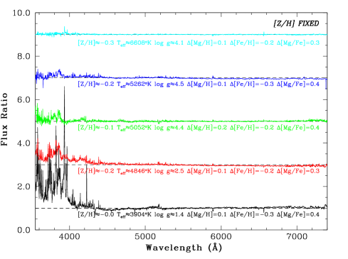
Figure 9: Ratios of pairs of MILES spectra showing the increasing importance of abundance pattern variations for cooler temperature stars. The plots are at fixed [Z/H] (typically around -0.2, estimated using equation 6), but varying [Mg/H] and [Fe/H] and are successively offset by 2.0 to avoid overlap. The star parameters are listed under each plot.

The spectral ratios shown in Section 4 illustrate that the impact of abundance variations on the blue region of the spectrum decreases with increasing temperature. This is seen when ratios of stars at fixed [Z/H], but varying [Fe/H] and [Mg/H] are plotted in order of increasing temperature in Fig. 9, which show decreasing variations with increasing temperature. This result is larger than the uncertainties due to stellar parameters, assessed from studies of similar stars. Therefore, study of abundance effects in the blue region of the spectrum is particularly important for cool stars.

6 Conclusions

The effects of element abundance changes on the strengths of spectral features in the spectra of different types of stars have been investigated. Theoretical response functions, widely used to measure abundance patterns in observed stellar populations, are tested against empirical data for stars from the MILES stellar library with measured abundances of [Fe/H] and [Mg/Fe]. Using the empirical [Mg/Fe] measurements from M11 as a proxy for overall [$\alpha$/Fe] values, the following results are found from these tests.

1. For K05 response functions the Fe sensitive features largely follow the observations, whereas H$\gamma$ and H$\delta$ features show systematically different behaviour between theoretical predictions and empirical observations. For the H$\gamma$ and H$\delta$ features, warm stars show a wider range of indices than predicted, whereas the opposite is true for cool stars. Indices sensitive to other elements show weaker trends, with larger scatter about the one-to-one lines (e.g. Mgb and Mg₂). The calcium sensitive feature (Ca4227) shows negligible trend, implying that additional factors affect this index apart from overall [$\alpha$/Fe].

2. For H02 response functions similar results are found as for the K05 comparisons, however, the agreement between theory and observations is improved for the H$\gamma$ and H$\delta$ features in cool stars when H02 response functions are used.

3. It is important to compile and obtain results for [Ca/Fe] measurement for MILES stars in future, to gain a better understanding of the influence of calcium on specific features such as Ca4227. Future measurements of carbon and nitrogen abundances in the stars studied in this paper are also important to obtain from high resolution spectra, in order to better understand the element responses of CN₁, CN₂, Ca4227 and other features.

4. For W12 star response functions (used in L09), together with K05 [Z/H] overall metallicity responses, similar patterns are found. These W12 star response functions could also be used for comparing many more stars to explore small changes in [$\alpha$/Fe] only. This showed typically a large scatter between normalised observations and normalised theoretical predictions, with weak trends about the one-to-one line for Mg₂, Mgb and NaD indices.

5. Full spectrum comparisons show that changes in the blue part of the spectrum are largely due to changes in [Fe/H] abundance. These changes decrease with increasing star temperature.

6. Overall [Z/H] is not always the most appropriate way to rank stars, since abundances of individual elements have important effects on emergent spectra and in general this is particularly important in the blue part of the spectra of cool stars, where Fe, C and N abundances strongly affect the spectral shape.

7. The spectral results so far indicate the need for deeper observational and theoretical studies of the blue part of stellar spectra, to search for more measurable metallicity indicators, senitive to iron abundance and to other element abundances in different types of stars. For example, indices in the blue have been defined by Rose (1994); Serven, Worthey & Briley (2005). We will explore this direction in a future paper.

In summary, this current work shows that theoretical response functions of K05 and H02 work quite well for most Lick spectral indices, with the exception of systematic offsets in the H$\gamma$ and H$\delta$ features, when compared to observed stars. This effect is important for individual stars and to a lesser extent for stellar population analysis, where the opposite systematics of warm and cool stars partially compensate for each other. The response functions need to be applied in a careful and limited way, taking into account the expected spread of values and types of indices, on an index-by-index basis. If response functions are applied automatically in a single method and for unlimited abundance variations, then they will produce spurious results in derived abundance patterns and in stellar population ages.

Appendix A Parameters for three categories of MILES stars.

This appendix shows tables of data for 7 CD, 31 TO and 13 CG stars, used in testing the K05 and H02 response functions in this paper, and plotted in Figs. 1 & 2. Details of these measurements are given Section 2.3. The [Mg/Fe] ratios are from M11. All 25 Lick indices are available in the on-line version.

Table 7: Tables of data for stars corresponding to the base model $T_{\rm eff}$ and $\log~{}g$ values in K05, for CD, TO and CG stars, from a 5Gyr old population.’M’ in column 7 denotes the MILES star number. All 25 Lick indices are available in the on-line version.

CD stars. Model=($T_{\rm eff}$=4575.0,$\log~{}g$=4.60)
No.	Name	$T_{\rm eff}$	$\log~{}g$	[Fe/H]	[Mg/Fe]	M	H$\delta_{A}$	H$\delta_{F}$	CN1	CN2	Ca4227	G4300	H$\gamma_{A}$	H$\gamma_{F}$
1	HD032147	4658	4.47	0.020	-0.056	168	-7.127	-1.370	0.101	0.150	3.527	5.809	-10.765	-3.638
2	HD131977	4501	4.70	0.020	0.124	532	-6.714	-1.176	0.025	0.076	4.021	5.471	-10.360	-3.266
3	HD156026	4541	4.54	-0.370	0.157	625	-5.710	-0.976	-0.021	0.034	4.642	4.967	-9.665	-3.166
4	HD103932	4510	4.57	0.160	-0.049	426	-6.926	-1.156	0.058	0.113	4.356	5.620	-11.064	-3.831
5	BD+430699	4608	4.52	-0.600	0.237	115	-5.430	-1.000	-0.002	0.038	3.183	5.331	-8.960	-3.053
6	HD021197	4616	4.59	0.300	-0.098	117	-6.463	-1.072	0.049	0.103	4.491	5.558	-11.053	-3.551
7	HD108564	4594	4.67	-1.090	0.516	442	-3.606	-0.158	-0.016	0.026	3.105	4.949	-7.847	-2.786
TO stars. Model=($T_{\rm eff}$=6200.0,$\log~{}g$=4.10)
No.	Name	$T_{\rm eff}$	$\log~{}g$	[Fe/H]	[Mg/Fe]	M	H$\delta_{A}$	H$\delta_{F}$	CN1	CN2	Ca4227	G4300	H$\gamma_{A}$	H$\gamma_{F}$
1	BD+342476	6205	4.12	-2.050	0.187	491	4.391	3.402	-0.089	-0.057	0.110	-0.307	3.953	3.419
2	HD000400	6205	4.12	-0.330	0.106	7	2.798	2.492	-0.083	-0.057	0.480	2.991	0.674	2.028
3	HD009826	6134	4.09	0.110	0.115	63	2.318	2.270	-0.080	-0.053	0.650	3.500	-0.108	1.831
4	HD014938	6153	4.04	-0.350	0.115	86	2.573	2.427	-0.071	-0.042	0.393	2.536	0.672	2.124
5	HD016673	6253	4.28	0.050	0.045	92	2.721	2.487	-0.085	-0.055	0.597	3.067	0.614	2.076
6	HD043318	6224	3.93	-0.150	0.059	213	2.861	2.550	-0.081	-0.054	0.337	2.866	1.055	2.356
7	HD074000	6166	4.19	-2.020	0.377	310	3.832	3.165	-0.079	-0.050	0.160	-0.049	3.465	3.117
8	HD076910	6275	4.10	-0.500	0.184	328	4.087	3.201	-0.089	-0.056	0.292	1.576	2.806	3.126
9	HD084937	6228	4.01	-2.170	0.440	363	4.460	3.589	-0.091	-0.062	0.049	-0.351	4.089	3.512
10	HD089744	6219	3.95	0.230	0.009	384	2.592	2.361	-0.077	-0.049	0.628	3.356	0.207	2.071
11	HD097916	6238	4.03	-0.990	0.454	405	4.690	3.559	-0.093	-0.058	0.264	0.847	3.693	3.587
12	HD102870	6109	4.20	0.170	-0.007	422	1.924	2.074	-0.070	-0.043	0.678	3.793	-0.686	1.556
13	HD107213	6298	4.01	0.290	0.133	438	2.816	2.505	-0.082	-0.053	0.488	3.476	0.321	2.122
14	HD114642	6249	3.90	-0.180	0.080	464	3.993	3.011	-0.095	-0.063	0.433	2.310	2.170	2.999
15	HD142860	6272	4.17	-0.160	0.070	576	3.045	2.622	-0.082	-0.050	0.477	2.619	1.515	2.526
16	HD159307	6198	3.90	-0.730	0.178	635	4.082	3.125	-0.096	-0.063	0.343	1.819	2.631	3.000
17	HD173667	6280	3.97	0.050	0.046	695	3.944	3.025	-0.097	-0.062	0.449	2.253	2.471	3.110
18	HD181096	6276	4.09	-0.260	0.119	716	3.523	2.879	-0.087	-0.057	0.396	2.400	1.700	2.725
19	HD215648	6167	4.04	-0.320	0.172	843	2.769	2.396	-0.078	-0.046	0.459	3.034	0.780	2.137
20	HD219623	6155	4.17	-0.040	0.026	868	2.057	2.211	-0.076	-0.049	0.646	3.664	-0.523	1.641
21	HD222368	6170	4.09	-0.150	0.131	888	2.671	2.371	-0.083	-0.054	0.519	3.088	0.616	2.160
22	HD338529	6165	4.06	-2.250	0.253	725	4.544	3.532	-0.093	-0.056	0.096	-0.399	4.295	3.510
23	HD097855	6260	4.05	-1.030	0.003	406	3.625	3.009	-0.081	-0.050	0.391	2.007	2.032	2.812
24	HD014221	6295	3.91	-0.350	0.041	83	4.154	3.265	-0.082	-0.050	0.353	1.615	2.761	3.366
25	BD+092190	6270	4.11	-2.860	0.477	348	4.914	3.817	-0.103	-0.068	0.061	-0.825	4.827	3.853
26	HD089995	6233	3.95	-0.340	-0.046	385	3.907	3.063	-0.088	-0.056	0.306	1.741	2.485	3.064
27	HD128429	6266	4.12	-0.130	0.267	518	3.408	2.864	-0.089	-0.054	0.417	2.550	2.023	2.834
28	HD173093	6268	4.09	-0.180	0.123	692	3.504	2.872	-0.086	-0.054	0.499	2.515	1.961	2.820
29	HD209369	6288	3.90	-0.280	0.153	822	3.843	2.851	-0.090	-0.059	0.383	1.938	2.582	3.183
30	HD218804	6261	4.05	-0.230	-0.054	862	4.078	3.219	-0.093	-0.060	0.464	1.714	2.982	3.294
31	BD+592723	6112	4.17	-2.020	0.528	876	3.609	3.108	-0.073	-0.048	0.152	0.044	3.090	2.808
CG stars. Model=($T_{\rm eff}$=4255.0,$\log~{}g$=1.90)
No.	Name	$T_{\rm eff}$	$\log~{}g$	[Fe/H]	[Mg/Fe]	M	H$\delta_{A}$	H$\delta_{F}$	CN1	CN2	Ca4227	G4300	H$\gamma_{A}$	H$\gamma_{F}$
1	HD131430	4190	1.95	0.100	-0.398	528	-7.221	-1.969	0.291	0.341	2.315	6.386	-11.045	-3.348
2	HD075691	4270	2.12	-0.050	0.015	321	-6.601	-1.619	0.220	0.267	1.929	6.321	-9.967	-3.006
3	HD113092	4283	1.95	-0.370	0.182	457	-4.085	-0.698	0.131	0.178	1.209	7.001	-8.716	-2.690
4	HD191046	4317	2.01	-0.650	0.474	755	-3.513	-0.834	0.076	0.111	1.036	6.952	-7.594	-2.424
5	HD020893	4340	2.04	0.080	-0.102	114	-5.997	-1.414	0.248	0.295	1.889	6.310	-10.137	-3.109
6	HD066141	4258	1.90	-0.300	0.061	289	-5.395	-1.068	0.167	0.216	1.614	6.564	-9.383	-3.176
7	HD083618	4231	1.74	-0.080	-0.086	357	-6.032	-1.450	0.189	0.236	2.143	6.322	-10.357	-3.131
8	HD124186	4347	2.10	0.240	0.002	499	-7.452	-1.896	0.327	0.375	2.077	6.382	-10.773	-3.453
9	HD130705	4336	2.10	0.410	-0.029	526	-7.541	-1.875	0.373	0.423	1.968	6.467	-10.970	-3.532
10	HD136726	4159	1.91	0.130	-0.087	549	-6.397	-1.562	0.217	0.270	2.677	6.222	-10.563	-3.199
11	HD154733	4200	2.09	0.000	-0.030	620	-6.444	-1.494	0.237	0.289	2.382	6.048	-10.153	-3.235
12	HD171443	4189	1.84	-0.080	0.009	682	-6.517	-1.529	0.263	0.319	2.168	6.618	-10.300	-3.348
13	M67$\_$F-108	4255	1.84	-0.090	0.016	919	-6.772	-1.755	0.238	0.288	2.422	6.308	-10.212	-3.253

Appendix B Tests with different abundance ratio trends.

For the results obtained in the main text we made the assumptions that all $\alpha$-element to iron ratios [$\alpha$/Fe] track the value of [Mg/Fe] and that carbon and nitrogen track iron. In this appendix we test these approximations using published data for samples of dwarf and giant stars. We fit mean trends to these data, to work out how element X varies with Mg or Fe, as a function of [Fe/H]. Table B1 shows these fits, ranges and references. Fig. B1 shows these mean relations in graphical form. The data from which these relations were obtained are plotted in the published papers (Soubiran & Girard 2005 - hereafter SG05; Luck & Heiter 2006 - hereafter LH06; Luck & Heiter 2007 - hereafter LH07). These consist of at least 415 dwarf stars from SG05 (see their table 3), 216 dwarf star from LH06 (see their tables 2 and 3), and $\sim$298 giant stars from LH07 (see their tables 4, 5 and 7).

Table 8: Polynomial fits for elements X showing how [X/Fe] varies with [Fe/H] on average, for elements modelled in the response function tables tested. The fitted datasets are indicated in the column headed ’References’, the numbers of stars fitted are shown in the column headed ’#’ and the rms deviations from the fit are shown in the final column, in dex.

Polynomial fit	[Fe/H] range	References	#	rms
DWARFS
$[MgFe]=$ 0.0624+0.0110[Fe/H]+0.4672[Fe/H]2-0.2692[Fe/H]3-0.3746[Fe/H]4	-1.2 to +0.5	SG05+LH06	818	0.096
$[Ca/Fe]=$ 0.0254-0.1261[Fe/H]+0.0930[Fe/H]2-0.0024[Fe/H]3	-1.2 to +0.5	SG05+LH06	743	0.061
$[Si/Fe]=$ 0.0419-0.1240[Fe/H]+0.1409[Fe/H]2+0.0073[Fe/H]3	-1.2 to +0.5	SG05+LH06	842	0.068
$[Ti/Fe]=$ 0.0412-0.0649[Fe/H]+0.3384[Fe/H]2+0.2060[Fe/H]3	-1.2 to +0.5	SG05+LH06	731	0.088
$[Na/Fe]=$ 0.0233+0.0757[Fe/H]+0.5329[Fe/H]2+0.4258[Fe/H]3	-1.2 to +0.3	SG05	567	0.080
$[O/Fe]=$ 0.1004-0.7273[Fe/H]-1.1294[Fe/H]2-0.5616[Fe/H]3	-1.2 to +0.3	SG05	415	0.125
GIANTS
$[Mg/Fe]=$ 0.0859+0.0361[Fe/H]+0.8155[Fe/H]2+0.0894[Fe/H]3	-0.6 to +0.35	LH07	298	0.103
$[Ca/Fe]=$ -0.0533-0.2468[Fe/H]-0.3619[Fe/H]2-0.7604[Fe/H]3	-0.6 to +0.35	LH07	294	0.080
$[Si/Fe]=$ 0.1365+0.0557[Fe/H]+0.6138[Fe/H]2-0.2128[Fe/H]3-0.6167[Fe/H]4	-0.6 to +0.35	LH07	291	0.064
$[Na/Fe]=$ 0.1283+0.1647[Fe/H]+0.4075[Fe/H]2+0.0971[Fe/H]3	-0.6 to +0.35	LH07	298	0.076
$[O/Fe]=$ 0.0477-0.4119[Fe/H]+1.1975[Fe/H]2+0.8401[Fe/H]3	-0.6 to +0.35	LH07	298	0.110
$[N/Fe]=$ 0.2060+0.1476[Fe/H]+0.0026[Fe/H]2-0.1319[Fe/H]3	-0.6 to +0.35	LH07	298	0.100
$[C/Fe]=$ -0.1568-0.2862[Fe/H]+1.0187[Fe/H]2+2.2720[Fe/H]3+1.7822[Fe/H]4	-0.6 to +0.35	LH07	298	0.103

The enhancements of $\alpha$ elements (O, Ca, Si and Ti) assumed in the main text are modified by trends for [X/Mg], derived from combining: [X/Mg]=[X/Fe]-[Mg/Fe], from Table 1B. Sodium is similarly modified by [Na/Mg]=[Na/Fe]-[Mg/Fe]. Nitrogen is treated as enhanced for giants, in this appendix, and scaled-solar for dwarfs (e.g. Takeda & Honda, 2005). Carbon, on the other hand, was originally assumed to follow iron in Section (3.1.1), which may be a good approximation for dwarfs (e.g. Takeda & Honda 2005, Da Silva et al. 2011) but not for giants (LH07). Therefore we modify our assumed carbon abundances for giants by adding [C/Fe] (from Table B1) to our original assumption.

In this way our measured [Mg/Fe] or [Fe/H] values for each star are then scaled by the above observed mean trends to generate estimates for other elements [X/Fe]. Applying these modified abundance patterns leads to similar relations as seen in Figs. 1 and 2, with the main exceptions being cool stars in the CN₁ and CN₂ bands, Ca4227 (affected by CN bands on one side), G4300 and to a lesser extent C₂4668. Tests of response functions for these features are therefore less certain, due to the greater impact of unknown C and N abundances. More robust tests of the responses for these 5 indices, in the blue part of the spectrum for cool stars, must await individual C and N element abundance measurements in those stars. The main results, regarding responses for iron features, Balmer features, magnesium and sodium features, remain intact. Contrast Fig. B2, which shows the H$\gamma$ and H$\delta$ indices and the 4 most uncertain features, with the same indices plotted in Fig. 1b and in Figs. 1d,e respectively.

For H$\gamma$ and H$\delta$ indices the robustness of our findings against uncertainties in individual element abundances points to the overall metallicity response as the cause of the observed difference between models and observations in Fig. 1(b). Here we test this. The good agreement of iron sensitive indices and others such as Ca4455 indicates that the spectral responses to overall metallicity ([Z/H]) in K05 and H02 are not significantly in error for those indices, in contrast to the case for H$\gamma$ and H$\delta$ indices. Table B2 compares the overall metallicity responses for these four Balmer indices, from K05 and H02. From this table we see that the spectral responses are smaller in H02 than in K05 (except for H$\delta_{A}$). For H$\delta_{A}$ the overall metallicity response is larger in H02 and this gives a worse fit to the observations (see Table 4). For the other three Balmer indices in Table B2, the smaller values of overall metallicity response in H02 lead to an improvement in the predictions for H$\gamma_{A}$, H$\gamma_{F}$ and H$\delta_{F}$ indices.

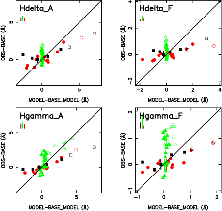
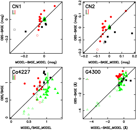
Figure 11: Testing the response functions of K05 by applying mean trends of element abundance ratios. The assumed element abundance ratios are modified by relations seen for stars in the local disk of the Milky Way. Comparison of normalised empirical versus normalised theoretical line strengths for standard Lick indices sensitive to four H Balmer lines and to four CN sensitive indices, in the stellar photospheres. Symbols as in Fig. 1(a), with cool dwarfs (CD, black squares), turn-off stars (TO, green triangles) and cool giants (CG, red circles).

Table 9: Balmer line spectral index responses (changes in $\AA$) to overall metallicity changes (by a factor of 2). From tables 12 and 14 in K05 and corresponding tables in H02.

		K05 [Z/H]	H02 [Z/H]
CD:	H$\delta_{A}$	-1.089	-0.704
	H$\delta_{F}$	-0.546	-0.280
	H$\gamma_{A}$	-1.381	-0.432
	H$\gamma_{F}$	-0.269	-0.099
CG:	H$\delta_{A}$	-1.533	-2.112
	H$\delta_{F}$	-1.252	-0.640
	H$\gamma_{A}$	-1.820	-0.720
	H$\gamma_{F}$	-0.534	-0.132

References

- Annibali et al. (2011) Annibali F., Grutzbauch R., Rampazzo R., Bressan A., Zeilinger W.W., 2011, A&A, 528, 19
- Bensby et al. (2005) Bensby T., Feltzing S., Lundström I., Ilyin I., 2005, A&A, 433, 185
- Carter et al. (2009) Carter D., et al., 2009, MNRAS, 397, 695
- Casagrande et al. (2006) Casagrande L., Portinari L., Flynn C., 2006, MNRAS, 373, 13 (Ce06)
- Cassisi et al. (2004) Cassisi S., Salaris M., Castelli F., Pietrinferni A., 2004, ApJ, 616, 498
- Cenarro et al. (2004) Cenarro A.J., Sanchez-Blazquez P., Cardiel N., Gorgas J., 2004, ApJ, 614, L101
- Cenarro et al. (2007) Cenarro A.J. et al., 2007, MNRAS, 374, 664
- Cenarro et al. (2009) Cenarro A.J., Cardiel N., Vazdekis A., Gorgas J., 2009, MNRAS, 396, 1895
- Cervantes & Vazdekis (2009) Cervantes J.L., Vazdekis A., 2009, MNRAS, 392, 691
- Clementini et al. (1999) Clementini G., Gratton R.G., Carretta E., Sneden C., 1999, MNRAS, 302, 22
- Coelho et al. (2005) Coelho P., Barbuy B., Melendez J., Schiavon R.P, Castilho B.V., 2005, A&A, 443, 735
- Coelho et al. (2007) Coelho P., Bruzual G., Charlot S., Weiss A., Barbuy B., Ferguson J.W., 2007, MNRAS, 382, 498
- Da Silva et al. (2011) Da Silva R., Milone A.C., Reddy B.E., 2011, A&A, 526, A71
- Delgado Mena et al. (2010) Delgado Mena E., Israelian G., González Hernández J.I., Bond J.C., Santos N.C., Udry S., Mayor M., 2010, ApJ, 725, 2349 (DM10)
- Ecuvillon et al. (2004) Ecuvillon A., Israelian G., Santos N.C., Mayor M., Villar V., Bihain G., 2004, A&A, 426, 619 (Ee04)
- Ecuvillon et al. (2006) Ecuvillon A., Israelian G., Santos N.C., Shchukina N.G., Mayor M., Rebolo R., 2006A&A, 445, 633 (Ee06)
- Falcón-Barroso et al. (2011) Falcón-Barroso J., Sánchez-Blázquez P., Vazdekis A., Ricciardelli E., Cardiel N., Cenarro A.J., Gorgas J., Peletier R.F., 2011, A&A, 532, 95
- Franchini et al. (2011) Franchini M., Morossi C., Di Marcantonio P., Malagnini M.L., Chavez M., 2011, ApJ, 730, 117
- Garcia Lopez et al. (1993) Garcia Lopez R.J., Rebolo R., Herrero A., Beckman J.E., 1993, ApJ, 412, 173 (GL93)
- Graves & Schiavon (2008) Graves G.J., Schiavon R.P., 2008, ApJS, 177, 446
- Grevesse & Sauval (1998) Grevesse N., Sauval A.J., 1998, Space Sci.Rev., 85, 161
- Houdashelt et al. (2002) Houdashelt M.L, Trager S.C., Worthey G., Bell R.A., 2002, BAAS, 201, 1405 (H02)
- James et al. (2006) James P.A., Salaris M., Davies J.I., Phillipps S., Cassisi S., 2006, MNRAS, 367, 339
- Jones (1999) Jones L.A., 1999, PhD thesis, University of North Carolina
- Kobayashi et al. (2006) Kobayashi C., Umeda H., Nomoto K., Tominaga N., Ohkubo T., 2006, ApJ, 653, 1145