Gaussian entanglement induced by an extended thermal environment

Abstract

We study stationary entanglement among three harmonic oscillators which are dipole coupled to a one-dimensional or a three-dimensional bosonic environment. The analysis of the open-system dynamics is performed with generalized quantum Langevin equations which we solve exactly in Fourier representation. The focus lies on Gaussian bipartite and tripartite entanglement induced by the highly non-Markovian interaction mediated by the environment. This environment-induced interaction represents an effective many-parties interaction with a spatial long-range feature: a main finding is that the presence of a passive oscillator is detrimental for the stationary two-mode entanglement. Furthermore, our results strongly indicate that the environment-induced entanglement mechanism corresponds to uncontrolled feedback which is predominantly coherent at low temperatures and for moderate oscillator-environment coupling as compared to the oscillator frequency.

I Introduction

Entanglement is a subtle feature of composite quantum systems, which is invariant under local operations, i.e., operations that act solely upon one constituent. Not considering protocols for entanglement swapping, entangling two subsystem requires an interaction between them horodecki20091 . Such interaction need not be direct, but may be mediated by a further quantum system or even a heat bath, despite that environmental degrees of freedom generally cause decoherence zurek2003 which is detrimental to entanglement. For example, the interaction with a common heat bath can entangle two otherwise uncoupled systems even in the weakly dissipative Markovian regime braun20021 ; plenio20021 ; benatti20031 ; benatti20101 by making use of decoherence-free subspaces that include entangled states doll20061 ; doll20071 ; shiokawa20091 ; wolf20111 ; kajari20121 or by correlated quantum noise that provides non-Markovian effects horhammer20081 ; zell20091 ; vasile20101 ; fleming20121 ; correa20121 . Also more involved system-environment interactions such as an exponential-like coupling duarte20091 ; valente20101 , as well as dissipative engineering techniques krauter20111 have been proposed for this issue. Given these multi-faceted behavior, it is intriguing to investigate entanglement between quantum systems in a more general dissipative scenario.

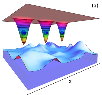
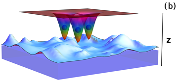
Figure 1: Oscillator-environment configuration considered in this work. Three oscillators are confined to the direction indicated by the arrow; in the 1D arrangement (a) the $x$-direction, while in the 3D configuration (b), the oscillators move only along the $z$-direction. The interaction between the oscillators is mediated by a bosonic field, which also causes decoherence and quantum dissipation.

In the present work, we investigate the setup sketched in Fig. 1 and explore the influence of thermal relaxation on the creation of stationary entanglement between three independent oscillators whose equilibrium positions are spatially separated, such that the indirect interaction mediated by the bath is retarded. In particular we address two issues. The first one is the bath-induced entanglement formation between two oscillators in the presence of a further oscillator. The second one is the characterization of the resulting stationary tripartite entanglement. We investigate both one-dimensional (1D) and three-dimensional (3D) environments, where the former is restricted to a linear arrangement of the three oscillators. Our model does not possess decoherence-free subspaces and, thus, any emerging entanglement must stem from the environment-mediated interaction which at the same time induces decoherence and quantum dissipation. A most important feature of an extended environment is its dispersion relation which implies a finite signal transmission velocity and, thus, causes retardation effects. They may lead to an entanglement decay in several stages doll20061 ; doll20071 or to a limiting distance for bath-induced two-mode entanglement zell20091 . Moreover, the dissipative quantum dynamics acquires an additional non-Markovian influence, which in our case is rather crucial because otherwise each oscillator would eventually reach its own Gibbs state and, thus, the total state would be separable.

Our paper is organized as follows. In Sec. II we define our model and derive within a quantum Langevin approach the main expressions and concepts used later for the numerical computations, which tare presented and discussed in Sec. III, where two-mode and three-mode entanglement is studied as a function of the main parameters of the model. Conclusions are drawn in Sec. IV. Some rather lengthy derivations have been deferred to the appendix.

II The model system and equilibrium state

We employ a generalized Caldeira-Leggett model weiss1999 ; leggett19871 ; hanggi19901 to capture thermal relaxation of the oscillators, which can be derived from first principles unruh19891 ; kohler20121 . We focus on the resulting stationary Gaussian entanglement that stems from the quadratic form of the Hamiltonian. The microscopic model will be approximately quadratic if the oscillators remain in their equilibrium positions (which is compatible with the presence of the environment-interaction effects), such that we can take the long-wave approximation at lowest order. The choice of a Gaussian initial state for the reservoir guarantees the Gaussian nature of the final stationary state. We assume a sudden switch-on of the interaction between the oscillators and the bath, such that the initial state of the full system (oscillator modes plus environment) is a product state $\rho_{0}=\rho\otimes\rho_{B}$.

In the case of a system composed by $N$ harmonic modes, the Gaussian stationary state is determined up to irrelevant local displacements by the four $N\times N$ correlation matrices

$$C_{\bm{A}\bm{B}}(t-t^{\prime})=\frac{1}{2}\langle\bm{A}(t)\bm{B}^{T}(t^{\prime})+\bm{B}(t^{\prime})\bm{A}^{T}(t)\rangle_{\rho},$$

with $\bm{A},\bm{B}\in\{\bm{X},\bm{P}\}$ and where $\bm{X}$ and $\bm{P}$ denote column vectors with the position and momentum operators of the oscillators. The Gaussian stationary state is characterized by the $2N\times 2N$ covariance matrix

$${G}=\begin{bmatrix}C_{\bm{X}\bm{X}}(0)&C_{\bm{X}\bm{P}}(0)\\ C_{\bm{P}\bm{X}}(0)&C_{\bm{P}\bm{P}}(0)\end{bmatrix},$$ (1)

which contains the full information about the system fluctuations. To compute $C_{\bm{A}\bm{B}}$, we employ the quantum Langevin equation formalism widely used in the study of Brownian motion weiss1999 ; hanggi20051 , which we adapt to our case of an extended environment. Regarding the study of entanglement, remarkable achievements have reported been concerning its classification and quantification for Gaussian states giedke20011 ; adesso20071 . A similar analysis of entanglement have been recently carried out for three identical harmonic oscillators in an equilateral triangular arrangement that are directly coupled and in contact with a common bosonic field at zero temperature hsiang20131 . In the opposite scenario of infinitely separated oscillators, each of them are fundamentally surrounded by independent environments such that they might be at different temperatures. In this case, the behavior of the entanglement has been proved to be essentially different valido20131 .

II.1 Generalized Langevin equation

We consider three harmonic oscillators located at $\bm{R}_{\lambda}=\bm{r}^{0}_{\lambda}+\bm{r}_{\lambda}$, where $\lambda=1,2,3$, while $\bm{r}^{0}_{\lambda}$ and $\bm{r}_{\lambda}$ denote equilibrium positions and displacements, respectively. We attribute to each displacement a conjugate momentum $\bm{p}_{\lambda}$, and employ the notations $\bm{r}_{\lambda}:=(x_{\lambda},y_{\lambda},z_{\lambda})$ and $\bm{p}_{\lambda}:=(p_{x,\lambda},p_{y,\lambda},p_{z,\lambda})$. The oscillators are assumed to be independent of each other with anisotropic confinement. This situation can be modeled by coupling the oscillators to a free bosonic field. Following the above considerations, we model our setup by the system-bath Hamiltonian $H_{0}=H_{S}+H_{B}+H_{I}$, with the system and the bath contribution

$$H_{S}={} \sum_{\lambda=1}^{3}\bigg{(}\frac{\bm{p}_{\lambda}^{2}}{2m_{\lambda}}+\frac{1}{2}m_{\lambda}(\omega^{2}_{x,\lambda}x^{2}_{\lambda}+\omega^{2}_{y,\lambda}y^{2}_{\lambda}+\omega^{2}_{z,\lambda}z^{2}_{\lambda})\bigg{)},$$ (2)

$$H_{B}={} \sum_{\bm{k}}\hbar\omega_{\bm{k}}a^{\dagger}_{\bm{k}}a_{\bm{k}},$$ (3)

respectively, where $a^{\dagger}_{\bm{k}}$ and $a_{\bm{k}}$ are the usual bosonic creation and annihilation operators for the bath mode with wavevector $\bm{k}=(2\pi/L)\mathbb{Z}^{D}$. We assume that only one degree of freedom per oscillator is coupled to the bosonic field and, thus, experiences decoherence. While in 1D, this assumption appears natural, it can be realized in the 3D case by a strong anisotropy, $\omega_{x,\lambda}\ll\omega_{y,\lambda},\omega_{z,\lambda}$, such that the motion in $y$- and $z$-direction is frozen and can be ignored. The interaction between the central oscillators and the environment then takes the form

$$H_{I}=-\sum_{\lambda=1}^{3}x_{\lambda}\sum_{\bm{k}}g_{\bm{k}}\Big{(}a_{\bm{k}}e^{i\bm{k}\cdot\bm{R}_{\lambda}}+a^{\dagger}_{\bm{k}}e^{-i\bm{k}\cdot\bm{R}_{\lambda}}\Big{)},$$ (4)

with the coupling constants $g_{\bm{k}}$ doll20061 . A technically important simplification is provided by the assumption that $e^{i\bm{k}\cdot\bm{r}_{\lambda}}\ll 1$, which physically corresponds to the long-wave limit or the dipole approximation for which we find

$$H_{I}\cong-\sum_{\lambda=1}^{3}x_{\lambda}\sum_{\bm{k}}g_{\bm{k}}\Big{(}a_{\bm{k}}e^{i\bm{k}\cdot\bm{r}^{0}_{\lambda}}+a^{\dagger}_{\bm{k}}e^{-i\bm{k}\cdot\bm{r}^{0}_{\lambda}}\Big{)}.$$ (5)

When coupling the bosonic field to the oscillators a counter-term must be added if one likes to preserve the bare oscillator potential of Eq. (3). Finally, the full oscillator-environment Hamiltonian becomes $H_{B}+H_{I}\to H_{BI}$, where

$$\begin{split}H_{BI}={}&\sum_{\bm{k}}\frac{1}{2m_{\bm{k}}}\Big{(}p_{\bm{k}}+g_{\bm{k}}\sqrt{\frac{2m_{\bm{k}}}{\hbar\omega_{\bm{k}}}}\sum_{\lambda=1}^{3}x_{\lambda}\sin(\bm{k}\cdot\bm{r}^{0}_{\lambda})\Big{)}^{2}\\ +&\sum_{\bm{k}}\frac{m_{\bm{k}}\omega_{\bm{k}}^{2}}{2}\Big{(}x_{\bm{k}}-\frac{g_{\bm{k}}}{\omega_{\bm{k}}^{2}}\sqrt{\frac{2\omega_{\bm{k}}}{m_{\bm{k}}\hbar}}\sum_{\lambda=1}^{3}x_{\lambda}\cos(\bm{k}\cdot\bm{r}^{0}_{\lambda})\Big{)}^{2}.\end{split}$$ (6)

We have introduced the usual bosonic annihilation operator $a_{\bm{k}}=(m_{\bm{k}}\omega_{\bm{k}}x_{\bm{k}}+i\,p_{\bm{k}})/\sqrt{2\hbar m_{\bm{k}}\omega_{\bm{k}}}$ and its adjoint $a^{\dagger}_{\bm{k}}$. The coupling together with the counter-terms in our Hamiltonian (6) can be interpreted as minimal coupling theory with $U(1)$ gauge symmetry kohler20121 . Moreover, in field theoretical terms, the oscillators are coupled to the velocity of the bosonic field unruh19891 , which guarantees that the energy remains positive definite and prevents “runaway” solutions coleman19621 .

Associated to Hamiltonian (6) are equations of motion for the degrees of freedoms of both the oscillators and the environment. The dynamics of those of the oscillators, conditioned to the environmental state, are given by a quantum Langevin equation which follows from the exact Heisenberg equation of motion for $\bm{X}:=(x_{1},x_{2},x_{3})$ and which, after tracing out the environmental degrees of freedoms, read weiss1999 (for details see Appendix A)

$${M}\ddot{\bm{X}}+{\phi}\bm{X}+\frac{1}{\hbar}{\displaystyle\int_{-\infty}^{t}}d\tau{{\chi}}(t-\tau)\bm{X}(\tau)=\bm{F}(t),$$ (7)

where here the mass matrix ${M}$ is proportional to the unit matrix, ${M}_{\lambda\mu}=m\delta_{\lambda\mu}$, while the counter-term $\tilde{\Omega}_{\lambda\mu}$ is part of the potential matrix $\phi_{\lambda\mu}=m\omega^{2}_{\lambda}\delta_{\lambda\mu}+2\tilde{\Omega}_{\lambda\mu}$. The memory-friction kernel ${\chi}(t)$ has the form of a $3\times 3$ matrix, and $\bm{F}$ is the column vector with the fluctuating forces $F(\bm{r}^{0}_{\lambda},t):=F_{\lambda}(t)$ that act upon each oscillator. These forces depend on the position of the oscillators and the environment. Owing to their quantum nature, the forces are operators and commute with each other only for time-like separations, i.e., $[F_{\lambda}(t^{\prime}),F_{\mu}(t)]=0$ if $|\bm{r}^{0}_{\lambda}-\bm{r}^{0}_{\mu}|>c|t-t^{\prime}|$, where $c$ is the sound velocity of the environment (or the speed of light, in a corresponding optical setup) which enters via the dispersion relation $\omega_{\bm{k}}=c|\bm{k}|$. It relates to the memory-friction kernel via the Kubo formula

$${{\chi}}_{\lambda\mu}(t-t^{\prime})=-i\left\langle[F_{\lambda}(t),F_{\mu}(t^{\prime})]\right\rangle_{\rho_{B}}\Theta(t-t^{\prime}-|\Delta\bm{r}^{0}_{\lambda\mu}|/c),$$ (8)

where the Heaviside step function $\Theta$ reflects causality with a retardation stemming from the distance $\Delta\bm{r}^{0}_{\lambda\mu}:=\bm{r}^{0}_{\lambda}-\bm{r}^{0}_{\mu}$ between the oscillators $\lambda$ and $\mu$. The average has been taken with respect to the Gibbs state $\rho_{B}$ with temperature $T$, which ensures the Gaussian property exploited below. In the frequency domain, the real part of the symmetrized forces correlation $F_{\lambda}(t)F_{\mu}(t^{\prime})$ reads

$$\mathop{\mathrm{Re}}\left\langle{\bm{F}}(\omega)\bm{F}^{T}(\omega^{\prime})+{\bm{F}}(\omega^{\prime})\bm{F}^{T}(\omega)\right\rangle_{\rho_{B}}=4\pi\hbar\delta\left(\omega+\omega^{\prime}\right){\Gamma}(\omega)$$ (9)

with the matrix $\Gamma$ defined by its elements

$$\Gamma_{\lambda\mu}(\omega)={} -\frac{1}{\hbar}\mathop{\mathrm{Im}}\chi_{\lambda\mu}(\omega)\coth\left(\frac{\hbar\omega}{2k_{B}T}\right)$$

$$={} J_{\lambda,\mu}(|\omega|)\coth\left(\frac{\hbar|\omega|}{2k_{B}T}\right).$$ (10)

This expression relates the real part of $\langle\left[F_{\lambda}(t),F_{\mu}(t^{\prime})\right]\rangle$ (commutator) to $\langle\{F_{\lambda}(t),F_{\mu}(t^{\prime})\}\rangle$ (anti-commutator), and thus, implies a quantum fluctuation-dissipation relation for the force operators. Moreover, we have introduced the bath spectral density

$$J_{\lambda,\mu}(\omega)=\frac{\pi}{\hbar}\sum_{\bm{k}}g^{2}_{\bm{k}}\cos\left(\bm{k}\cdot\Delta\bm{r}^{0}_{\lambda\mu}\right)\delta\left(\omega-\omega_{\bm{k}}\right)$$ (11)

which allows us to write the renormalization terms in the convenient form

$$\tilde{\Omega}_{\lambda\lambda} = \frac{1}{\hbar}\sum_{\bm{k}}\frac{g_{\bm{k}}^{2}}{\omega_{\bm{k}}}=\frac{1}{\pi}\int_{0}^{\infty}\frac{J_{\lambda,\lambda}(\omega)}{\omega}d\omega,$$ (12)

$$\tilde{\Omega}_{\lambda\mu} = \frac{1}{\hbar}\sum_{\bm{k}}\frac{g_{\bm{k}}^{2}}{\omega_{\bm{k}}}\cos\left(\bm{k}\cdot\Delta\bm{r}^{0}_{\lambda\mu}\right)=\frac{1}{\pi}\int_{0}^{\infty}\frac{J_{\lambda,\mu}(\omega)}{\omega}d\omega.$$

With these relations, we can express the impact of the bath on the oscillators and their effective interaction, as well as non-Markovian memory effects in terms of the spectral density (11).

The non-diagonal potential renormalization (12) couples the oscillator coordinates $x_{\lambda}$ which, thus, are no longer the normal modes of our problem. Therefore, we introduce the transformation matrix ${O}$ which maps to the normal modes of the coupled oscillators, $\bm{Q}={O}\bm{X}$. Together with the according transformation for our matrices, we obtain for $\bm{Q}$ the Langevin equation

$${M}\ddot{\bm{Q}}+{\phi}_{D}\bm{Q}+\frac{1}{\hbar}{\displaystyle\int_{-\infty}^{t}}d\tau{{\Xi}}(t-\tau)\bm{Q}(\tau)=\bm{D}(t)$$ (13)

with the mass matrix ${O}{M}{O}^{T}=M$, the potential matrix ${\phi}_{D}={O}{\phi}{O}^{T}$, the susceptibility ${\Xi}(t)={O}{\chi}(t){O}^{T}$, and the fluctuation forces $\bm{D}(t)={O}\bm{F}(t)$, while the fluctuation-dissipation relation becomes

$$\mathop{\mathrm{Re}}\left\langle{\bm{D}}(\omega)\bm{D}^{T}(\omega^{\prime})+{\bm{D}}(\omega^{\prime})\bm{D}^{T}(\omega)\right\rangle_{\rho_{B}}=4\pi\hbar\delta\left(\omega+\omega^{\prime}\right){\Upsilon}(\omega)$$

with $\Upsilon(\omega)=-(1/\hbar)\mathop{\mathrm{Im}}{\Xi}(\omega)={O}^{T}\Gamma\left(\omega\right){O}.$ While the conservative part of the transformed Langevin equation (13) is now diagonal, the modes may still couple via the dissipation kernel ${\Xi}(t)$, unless the latter is diagonal as well. This can be achieved if ${\phi}$ and ${\chi}(t)$ commute at all times, which is the case if all oscillators have the same fundamental frequencies and are equally spaced, i.e., ${\phi}$ and ${\chi}(t)$ commute when the equilibrium positions of the oscillators form a equilateral triangle ($\Delta\bm{r}^{0}_{\lambda\mu}=R$ for all $\lambda\neq\mu$) because they are symmetric matrices and their product is also symmetric hsiang20131 . A further particular geometry is given when the oscillators are placed in an isosceles triangle. Then the normal mode corresponding to the relative motion of the oscillators placed at the ends of the unequal side of the triangle and the center of mass dynamics are independent of each other. We consider these distinct geometries in Sec. III. Furthermore, it follows from the rank-nullity theorem aitken1956 that the evolution of all normal modes will be subject to dissipation and noise unless all oscillators have the same frequency and are at the same place. Then their relative coordinate forms a decoherence-free subspace (shiokawa20091, ; kajari20121, ). In general however, i.e., for any other geometry, the oscillator-bath Hamiltonian does not possess a decoherence-free subspace.

Having developed the formal solution of the quantum Langevin equation (7), we are able to evaluate the covariance matrix (1) whose entries read

$$C_{\bm{X}\bm{X}}(0)={} \hbar\int\frac{d\omega}{2\pi}{\alpha}(\omega){\Gamma}(\omega){\alpha}(-\omega)^{T},$$ (14)

$$C_{\bm{X}\bm{P}}(0)={} C_{\bm{P}\bm{X}}(0)=m\hbar{\displaystyle\int}\frac{d\omega}{2\pi}\,i\omega\,{\alpha}(\omega){\Gamma}(\omega){\alpha}(-\omega)^{T},$$ (15)

$$C_{\bm{P}\bm{P}}(0)={} m^{2}\hbar{\displaystyle\int}\frac{d\omega}{2\pi}\,\omega^{2}\,{\alpha}(\omega){\Gamma}(\omega){\alpha}(-\omega)^{T},$$ (16)

where ${\alpha}(\omega)$ corresponds to the Fourier transformed of the left-hand side of the quantum Langevin equation (7). All the covariances contain the integration kernel ${K}\left(\omega\right)={\alpha}(\omega){\Gamma}(\omega){\alpha}(-\omega)^{T}$, while from the quantum fluctuation-dissipation relation (9) follows that ${K}\left(\omega\right)$ is completely characterized by the generalized spectral density $J_{\lambda,\mu}(\omega)$.

II.2 Generalized spectral density and integration kernel ${K}\left(\omega\right)$

We assume for the bosonic field the linear dispersion $\omega_{\bm{k}}=c|\bm{k}|$, which comprises the physical cases of acoustic phonons and a free electromagnetic field. Then it is possible to construct the spectral densities $J_{\lambda,\mu}(\omega)$ which is a necessary step for computing the full covariance matrix (1). A detailed derivation for the expressions introduced in this section can be found in Appendix B.

We shall focus on 1D and 3D environments with isotropic coupling between the oscillators and the bosonic field. For the coupling we choose $g^{2}_{\bm{k}}=m\hbar\gamma(\omega_{\bm{k}}/\omega_{c}^{d-1})c^{d}V_{\bm{k}}(d)e^{-\omega/\omega_{c}}$, where $d$ is the dimension of the environment, $V_{\bm{k}}$ is the number of field modes per $d$-dimensional $\bm{k}$-space volume, $\gamma$ is the coupling strength coupling, and $\omega_{c}$ is the cut-off frequency of the environmental spectrum. Eventually, the continuum limit $V_{\bm{k}}\to 0$ will be taken. Hence, we obtain the spectral densities

$$J^{1D}_{\lambda,\mu}(\omega) = \pi m\gamma\omega e^{-\omega/\omega_{c}}\cos(\omega|\Delta\bm{r}^{0}_{\lambda\mu}|/c),$$ (17)

$$J^{3D}_{\lambda,\mu}(\omega) = \frac{4\pi^{2}mc}{|\Delta\bm{r}^{0}_{\lambda\mu}|}\Big{(}\frac{\omega}{\omega_{c}}\Big{)}^{2}e^{-\omega/\omega_{c}}\sin(\omega|\Delta\bm{r}^{0}_{\lambda\mu}|/c).$$ (18)

Accordingly, the potential renormalizations become

$$\Omega^{1D}_{\lambda\mu} = \frac{m\gamma\omega_{c}}{1+(\omega_{c}|\Delta\bm{r}^{0}_{\lambda\mu}|/c)^{2}},$$ (19)

$$\Omega^{3D}_{\lambda\mu} = \frac{8m\pi\gamma\omega_{c}}{[1+(\omega_{c}|\Delta\bm{r}^{0}_{\lambda\mu}|/c)^{2}]^{2}}.$$ (20)

The imaginary part of the susceptibilities follows by inserting the spectral densities into Eq. (10), while their real parts are conveniently obtained via the Kramers-Kronig relations, so that we obtain

$$\chi^{1D}_{\lambda\mu}(t) = 4m\,\gamma\,\hbar\,\omega^{2}_{c}\Theta\left(t-|\Delta\bm{r}^{0}_{\lambda\mu}|/c\right)$$ (21)

$$\times\frac{\omega_{c}|\Delta\bm{r}^{0}_{\lambda\mu}|/c-t\omega_{c}}{[1+(\omega_{c}|\Delta\bm{r}^{0}_{\lambda\mu}|/c-t\omega_{c})^{2}]^{2}},$$

$$\chi^{3D}_{\lambda\mu}(t) = 8\pi m\,\gamma\,\hbar\,\frac{\omega_{c}c}{|\Delta\bm{r}^{0}_{\lambda\mu}|}\Theta(t-|\Delta\bm{r}^{0}_{\lambda\mu}|/c)$$ (22)

$$\times\Bigg{(}\frac{1-3(\omega_{c}|\Delta\bm{r}^{0}_{\lambda\mu}|/c+t\omega_{c})^{2}}{[1+(\omega_{c}|\Delta\bm{r}^{0}_{\lambda\mu}|/c+t\omega_{c})^{2}]^{3}}$$

$$-\frac{1-3(\omega_{c}|\Delta\bm{r}^{0}_{\lambda\mu}|/c-t\omega_{c})^{2}}{[1+(\omega_{c}|\Delta\bm{r}^{0}_{\lambda\mu}|/c-t\omega_{c})^{2}]^{3}}\Bigg{)}.$$

The non-exponential decay in time obeyed by the susceptibilities (memory kernels) describes non-Markovian dissipation zhang20121 , which will turn out as essential ingredient for stationary entanglement in our system. Moreover, the dimensionless parameter $|\Delta\bm{r}^{0}_{\lambda\mu}|\omega_{c}/c$ is also involved in the renormalization terms and generalized spectral densities. It compares two different time scales, on one the hand $|\Delta\bm{r}^{0}_{\lambda\mu}|/c$, that is the time of flight of a phonon or photon between two oscillators, and on the other hand $\omega_{c}^{-1}$ which represents the time scale during which memory effects decay. Surprisingly, the environment-mediated interaction, inherent in the susceptibilities and in the renormalization term, establishes an effective coupling between all oscillators irrespective of their distance. At fixed time, they decay polynomially in space at least as $\sim(|\Delta\bm{r}^{0}_{\lambda\mu}|\omega_{c}/c)^{3}$ and $\sim(|\Delta\bm{r}^{0}_{\lambda\mu}|\omega_{c}/c)^{8}$ for the 1D and the 3D reservoir, respectively. Although this interaction possesses long-range features, we shall see that the characteristic length of the entanglement correlation is determined by $|\Delta\bm{r}^{0}_{\lambda\mu}|\omega_{c}/c$, in agreement with Ref. zell20091 .

Once we have the susceptibilities and the renormalization terms at hand, we can compute the matrices ${\alpha}(\omega)$ for which we obtain

$${\alpha}^{1D}_{\lambda\mu}(\omega) = m(\omega_{\lambda}^{2}-\omega^{2})\delta_{\lambda\mu}-m\gamma\omega\mathop{\mathrm{Re}}\left(g(\omega)-g(-\omega)\right)$$ (23)

$$+\pi m\,\gamma\,\omega\,\mathop{\mathrm{Im}}\Big{[}\Theta(\omega)e^{-\left(1/\omega_{c}-i|\Delta\bm{r}^{0}_{\lambda\mu}|/c\right)\omega}$$

$$-\Theta(-\omega)e^{(1/\omega_{c}-i|\Delta\bm{r}^{0}_{\lambda\mu}|/c)\omega}\Big{]}$$

$$-i\pi m\gamma\omega\cos(|\Delta\bm{r}^{0}_{\lambda\mu}|\omega/c)e^{-|\omega|/\omega_{c}},$$

$${\alpha}^{3D}_{\lambda\mu}(\omega) = m(\omega_{\lambda}^{2}-\omega^{2})\delta_{\lambda\mu}-i4\pi^{2}m\gamma(c/|\Delta\bm{r}^{0}_{\lambda\mu}|)\Big{(}\frac{\omega}{\omega_{c}}\Big{)}^{2}$$ (24)

$$\times\sin(\omega|\Delta\bm{r}^{0}_{\lambda\mu}|/c)e^{-|\omega|/\omega_{c}}$$

$$-\frac{4\pi\,m\,\gamma\,c\,\omega^{2}}{\omega_{c}^{2}{|\Delta\bm{r}^{0}_{\lambda\mu}|}}\mathop{\mathrm{Im}}\left(g(\omega)+g(-\omega)\right)$$

$$-\frac{4\pi^{2}\,m\,\gamma\,c\,\omega^{2}}{\omega_{c}^{2}{|\Delta\bm{r}^{0}_{\lambda\mu}|}}\mathop{\mathrm{Re}}\Big{[}\Theta(\omega)e^{-(1/\omega_{c}-i|\Delta\bm{r}^{0}_{\lambda\mu}|/c)\omega}$$

$$+\Theta(-\omega)e^{(1/\omega_{c}-i|\Delta\bm{r}^{0}_{\lambda\mu}|/c)\omega}\Big{]},$$

where

$$g(\omega)=e^{-(1-i\omega_{c}|\Delta\bm{r}^{0}_{\lambda\mu}|/c)\omega/\omega_{c}}\Gamma[0,-(1-i\omega_{c}|\Delta\bm{r}^{0}_{\lambda\mu}|/c)\omega/\omega_{c}],$$

and $\Gamma(0,x)$ is the incomplete gamma function. With these expressions, we readily obtain the elements of the stationary correlation matrix. Moreover, the dimension-dependent integration kernels $K(\omega)$ can be evaluated to read

$${K}_{\eta,\beta}^{1D}(\omega) = \pi m\gamma\,\omega\,\coth\left(\frac{\hbar\omega}{2k_{B}T}\right)e^{-|\omega|/\omega_{c}}$$

$$\times\sum_{\lambda,\mu}\cos\left(\omega|\Delta\bm{r}^{0}_{\lambda\mu}|/c\right)$$

$$\times\frac{\left(\hbox{adj}[{\alpha}^{1D}(\omega)]\right)_{\eta\lambda}\left(\hbox{adj}[{\alpha}^{1D}(-\omega)^{T}]\right)_{\mu\beta}}{|{\alpha}^{1D}(\omega)||{\alpha}^{1D}(-\omega)^{T}|},$$

$$\begin{split}{K}_{\eta,\beta}^{3D}(\omega)={}&4\pi^{2}m\gamma\Big{(}\frac{\omega}{\omega_{c}}\Big{)}^{2}\coth\left(\frac{\hbar\omega}{2k_{B}T}\right)e^{-|\omega|/\omega_{c}}\\ &\times\sum_{\lambda,\mu}\left(c/|\Delta\bm{r}^{0}_{\lambda\mu}|\right)\sin\left(\omega|\Delta\bm{r}^{0}_{\lambda\mu}|/c\right)\\ &\times\frac{\left(\hbox{adj}[{\alpha}^{3D}(\omega)]\right)_{\eta\lambda}\left(\hbox{adj}[{\alpha}^{3D}(-\omega)^{T}]\right)_{\mu\beta}}{|{\alpha}^{3D}(\omega)||{\alpha}^{3D}(-\omega)^{T}|},\end{split}$$ (26)

where $\hbox{adj}[{\alpha}]$ and $|{\alpha}|$ are the adjoint and the determinant of ${\alpha}$. With these expressions, we have achieved a closed, albeit quite complicated form for the susceptibilities. Nevertheless, having the analytic expressions at hand, certainly facilitates the numerical evaluation of the covariance matrices (14)–(16).

III Thermal entanglement induced by isotropic substrates

Having derived the solution of the quantum Langevin equations, we turn to the entanglement among the oscillators induced by the non-Markovian dissipative dynamics. We focus on the quantum regime which requires low temperatures, $k_{B}T\ll\hbar\omega_{\lambda}$. In order to have the environment playing a constructive role, it must couple strongly to the oscillators, such that the quality factors $Q_{\lambda}=\omega_{\lambda}/\gamma\sim 1$–$10$ are rather small. In this regime, the dissipative oscillator dynamics is strongly non-Markovian. In the numerical evaluations of our analytical expressions, we use the typical units for nano oscillators, i.e., for masses $m=10^{-16}$ kg, for frequencies $\Omega=1$ GHz, and for distances $R=10$ nm. Realistic values for an environment realized by a solid-sate substrate are a cutoff frequency (Debye frequency) corresponding to $\hbar\omega_{c}=6.58\cdot 10^{-2}$ meV and $c=3000$ m/s for the speed of sound.

We characterize the Gaussian entanglement between two generic modes $\mathcal{X}$ and $\mathcal{Y}$ by the logarithmic negativity (vidal20021, )

$$E_{N}\left(\rho_{\mathcal{X}\mathcal{Y}}\right)=\mathop{\text{max}}\{0,-\ln\left(2\nu_{-}\right)\},$$ (27)

where $\mathcal{X}$ and $\mathcal{Y}$ represent one of the three oscillators, henceforth labeled by $\mathcal{A}$, $\mathcal{B}$, and $\mathcal{C}$. Here, $\nu_{-}$ is the lowest symplectic eigenvalue of the partial transpose covariance matrix ${G}^{T_{\mathcal{Y}}}$ (see Appendix D for details) corresponding to the reduced density matrix $\rho_{\mathcal{X}\mathcal{Y}}$ of the two modes. Regarding the analysis of three-mode Gaussian entanglement, there is no generally accepted measure of tripartite entanglement for arbitrary mixed states. Nonetheless it is possible to characterize it by a classification scheme that assigns each state to one of five separability classes (giedke20011, ), which range from fully inseparable states (class 1) to mixed tripartite product states (class 5). For details see Appendix D.

Even though our focus lies on entanglement, we investigate for completeness also the quantum fidelity $\mathcal{F}\left(\rho,\rho^{C}\right)$ of the thermal state $\rho^{C}\propto e^{-H_{S}/k_{B}T}$ as a function of the spatial degrees of freedom and temperature. In Ref. marian20121 an analytical expression for $\mathcal{F}\left(\rho,\rho^{\prime}\right)$ was found for arbitrary $n$-mode Gaussian states. In our case, it becomes

$$\begin{split}\mathcal{F}\left(\rho,\rho^{C}\right)={}&\prod_{i=1}^{n}\frac{2}{\left(\nu_{i}+\nu^{C}_{i}\right)^{2}}\left[\nu_{i}\nu^{C}_{i}+\frac{1}{4}\right.\\ &+\left.\sqrt{\left(\nu_{i}^{2}-\frac{1}{4}\right)\left(\left(\nu^{C}_{i}\right)^{2}-\frac{1}{4}\right)}\right],\end{split}$$ (28)

where $\nu_{i}$ and $\nu^{C}_{i}$ are the symplectic eigenvalues of the covariance matrix of $\rho$ and $\rho^{C}$, respectively. Notice that here the symplectic eigenvalues are different from those used for the logarithmic negativity, because they are derived without partial transposition.

In previous works duarte20091 ; valente20101 on environment-induced entanglement, it was found that when the oscillators are very close each other, the most significant influence of the environment is to mediate an effective interaction between the oscillators, while decoherence becomes relevant mainly at higher temperatures. Moreover, it has been pointed out that for identical oscillators, entanglement creation may stem from a decoherence-free subspace shiokawa20091 ; kajari20121 . Here, we consider oscillators with different frequencies. Additionally, the Hamiltonian has no symmetries that would support decoherence-free subspaces unless the distance between the oscillators vanishes. This implies that the stationary entanglement has its roots in an environment-mediated interaction. From the Langevin equation (7), we see that this interaction enters as a renormalization potential or via dissipative effects, which we interpret as stochastic feedback between the oscillators.

III.1 Two-mode entanglement

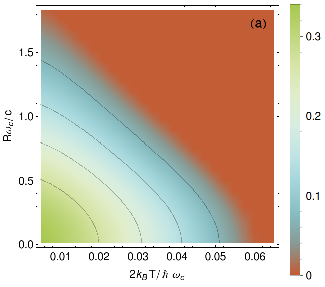
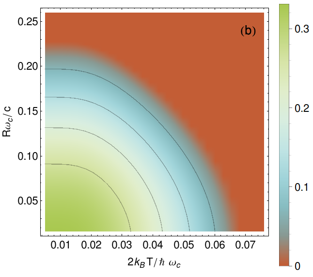
Figure 2: (Color online) Stationary two-mode entanglement measured by the logarithmic negativity (27) as a function of oscillator distance $R$ and temperature $T$ for a (a) 1D and a (b) 3D environment. The oscillator frequencies are $\omega_{\mathcal{A}}=7.2\Omega$, and $\omega_{\mathcal{B}}=13.2\Omega$, while the dissipation is $\gamma=5\Omega$.

We start by addressing the two-mode entanglement between the oscillators $\mathcal{A}$ and $\mathcal{C}$, placed at a distance $\Delta\bm{r}^{0}_{\mathcal{A}\mathcal{C}}=R$, in the absence of oscillator $\mathcal{B}$. This is equivalent to putting oscillator $\mathcal{B}$ at infinite distance, $\Delta\bm{r}^{0}_{\mathcal{A}\mathcal{B}}=\Delta\bm{r}^{0}_{\mathcal{B}\mathcal{C}}\rightarrow\infty$. Figure 2 depicts $E_{N}(\rho_{\mathcal{A}\mathcal{C}})$ for this case as function of the distance $R$ and the temperature $T$ for a 1D and a 3D environment, respectively. Although the environment induces a long-range interaction [cf. the susceptibilities (23) and (24)] with a polynomial decay in both space and time, we recover a central result of Ref. zell20091 : The correlation length is given by $R\approx\omega_{c}/c$, while the entanglement vanishes at a finite distance $R_{0}$ which mainly depends on the temperature, while being almost independent of the dissipation strength $\gamma$. Still a larger $\gamma$ supports the effective interaction required for entanglement creation horhammer20081 ; duarte20091 , but also increases decoherence which acts towards separability. Nevertheless, as expected, entanglement eventually disappears with increasing $\gamma$.

In 3D, entanglement generally appears more robust against thermal fluctuations, which is consistent with previous findings for qubits doll20061 ; doll20071 . A qualitative explanation for this is the super-Ohmic character of the 3D spectral density of the bath which leads to stronger memory effects zhang20071 . In turn, in the 1D case, entanglement is less affected by increasing the spatial separation $R$, which relates to the decay of the susceptibility as a function of the distance as we mentioned above: As function of $R$, the susceptibility $\chi^{3D}(t)$ decreases, at least, five orders stronger than $\chi^{1D}(t)$. Thus, the effective interaction at large distance in 3D is weaker than in 1D. In both cases, the well-defined finite distance between the entangled oscillators indicates that our mechanism for two-mode entanglement relies on memory effects. Otherwise, we would expect a polynomial or exponential decay of the two-mode correlations with increasing distance. This supports the idea that the environment-induced interaction represents a kind of feedback between oscillators which is predominantly coherent when only low energy environmental modes are thermally excited, i.e., for $k_{B}T\ll\hbar\omega_{c}$. Moreover, depending on the separation, the coupling strength with the environment is not too large to cause a strong decoherence.

We already discussed that the effective interaction potential provided by the renormalization term $\tilde{\Omega}$ is crucial, but cannot explain fully the amount of entanglement observed. In order to underline this statement, let us assume that dissipation and noise are negligible, so that the problem reduces to two harmonic oscillators at thermal equilibrium with interaction potential ${\phi}$. Then identical oscillators with equal frequencies $\omega_{\mathcal{A}}=\omega_{\mathcal{C}}=\Omega$ coupled at equal position to a substrate ($R\rightarrow 0$), will be entangled under a condition ludwig20101 that in our case can be written as

$$\left(2N^{1D}_{+}+1\right)\left(2N^{1D}_{-}+1\right)\left(1-\frac{2\gamma\omega_{c}}{\Omega^{2}[1+(\omega_{c}R/c)^{2}]}\right)<1,$$

(29)

$$\left(2N^{3D}_{+}+1\right)\left(2N^{3D}_{-}+1\right)\left(1-\frac{16\pi\gamma\omega_{c}}{\Omega^{2}[1+(\omega_{c}R/c)^{2}]^{2}}\right)<1,$$

where $N^{1D,3D}_{\pm}=[e^{\hbar\Omega^{1D,3D}_{\pm}/k_{B}T}-1]^{-1}$ denotes the bosonic thermal occupation of normal modes with the frequencies

$$\Omega^{1D}_{\pm} = \Omega\sqrt{1+\frac{2\gamma\omega_{c}}{\Omega^{2}}\pm\frac{2\gamma\omega_{c}}{\Omega^{2}[1+(\omega_{c}R/c)^{2}]}}\,,$$ (31)

$$\Omega^{3D}_{\pm} = \Omega\sqrt{1+\frac{16\pi\gamma\omega_{c}}{\Omega^{2}}\pm\frac{16\pi\gamma\omega_{c}}{\Omega^{2}[1+(\omega_{c}R/c)^{2}]^{2}}}.$$ (32)

Notice that the conditions (III.1) and (III.1) result from an expansion of the symplectic eigenvalues to first order in $\gamma\omega_{c}/\Omega^{2}$ implying $\gamma\omega_{c}<\Omega^{2}$, for which the left-hand side of these expressions are strictly positive when neglecting dissipation and quantum noise riseborough19851 . These conditions demonstrate that $R$ plays an important role for the entanglement creation as can be appreciated in Fig. 2. Still, these analytic considerations over-estimate the influence of $R_{0}$ as a quantitative comparison with the numerically evaluated expressions demonstrates (not shown). Although, we find that the available entanglement generated by the effective potential $\tilde{\Omega}$ does not display most of the characteristics of the stationary entanglement discussed above, is still relevant in the transient dynamics benatti20101 . In the long-time limit, both the numerical data and the analytical results for the susceptibilities indicate that the mechanism behind entanglement creation may be interpreted as uncontrolled feedback (encoded by the susceptibility) which relies on the non-Markovian dissipation.

III.2 Two-mode entanglement in the presence of a third oscillator

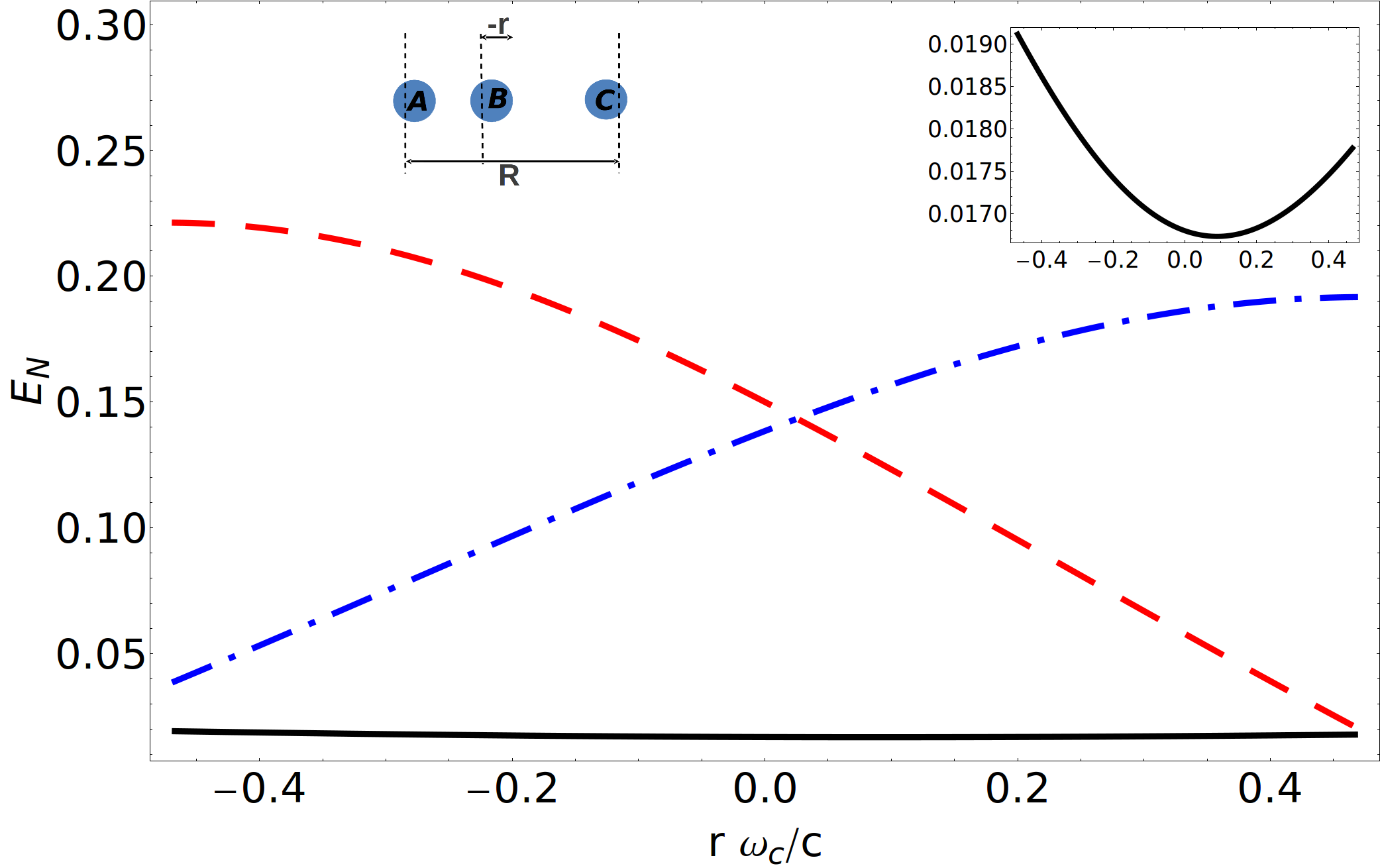
Figure 3: (Color online) Stationary two-mode entanglement in the linear arrangement quantified by the logarithmic negativities $E_{N}(\rho_{\mathcal{A}\mathcal{C}})$ (black solid line), $E_{N}(\rho_{\mathcal{A}\mathcal{B}})$ (red dashed), and $E_{N}(\rho_{\mathcal{B}\mathcal{C}})$ (blue dash-dotted) for $R\omega_{c}/c=0.933$. Temperature and damping are $k_{B}T/\hbar\omega_{c}=0.026$, $\gamma=5\Omega$, respectively, while the frequencies are $\omega_{\mathcal{A}}=7.2\Omega$, $\omega_{\mathcal{B}}=10.1\Omega$, and $\omega_{\mathcal{C}}=13.2\Omega$, where $\Omega=1$ GHz. The asymmetry between $E_{N}(\rho_{\mathcal{A}\mathcal{B}})$ and $E_{N}(\rho_{\mathcal{B}\mathcal{C}})$ is a consequence of choosing different oscillator frequencies. The entanglement between $\mathcal{A}$ and $\mathcal{B}$ is less sensitive to a moderate increase of temperature (not shown), because it involves the oscillators with the highest frequencies. The inset is a zoom that demonstrates the small quadratic increase of $E_{N}\left(\rho_{\mathcal{A}\mathcal{C}}\right)$.

We have already seen that the coupling to a common environment induces an effective interaction between oscillators and may create two-mode entanglement. In the case that more oscillators are in contact with the bath, we expect that additional effective interactions between any pair of oscillators emerge, provided that the oscillators are sufficiently close to each other, i.e., for distances $R\ll c/\omega_{c}$. It has been shown benatti20111 ; an20111 that for three qubits in contact with a common environment, the two-qubit entanglement for certain initial states persists in the long-time limit when coupling a further qubit to the substrate. Hence, the question arises how two-mode entanglement is affected by the presence of a third oscillators. We study two different configurations: The first one is a linear arrangement in which the three oscillators are coupled to a 1D environment with separations $\Delta\bm{r}^{0}_{\mathcal{A}\mathcal{C}}=R$, $\Delta\bm{r}^{0}_{\mathcal{A}\mathcal{B}}=R/2+r$, and $\Delta\bm{r}^{0}_{\mathcal{B}\mathcal{C}}=R/2-r$, where $0<r<R/2$, as is sketched in Fig. 3. We fix $R$ such that the outer oscillators $\mathcal{A}$ and $\mathcal{C}$ may be entangled or separable, depending on the other parameters. In the second configuration, the oscillators are in contact with a 3D reservoir. The oscillators $\mathcal{A}$ and $\mathcal{C}$ are again at distance $\Delta\bm{r}^{0}_{\mathcal{A}\mathcal{C}}=R$, but oscillator $\mathcal{B}$ is shifted by $r$ perpendicular to the line connecting $\mathcal{A}$ and $\mathcal{C}$, see sketch in Fig. 4. Thus, $\Delta\bm{r}^{0}_{\mathcal{B}\mathcal{C}}=\Delta\bm{r}^{0}_{\mathcal{A}\mathcal{B}}=[r^{2}+(R/2)^{2}]^{1/2}$.

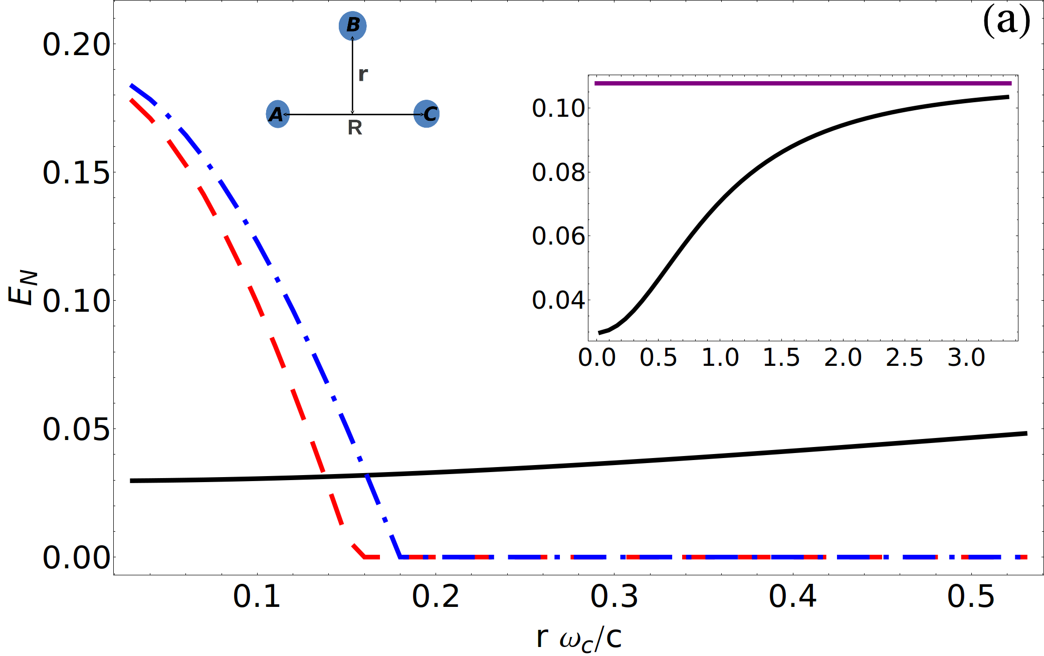
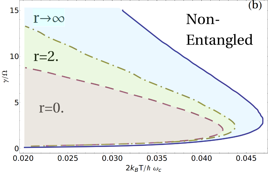
Figure 4: (Color online) (a) Stationary two-mode entanglement measured by the logarithmic negativities $E_{N}(\rho_{\mathcal{A}\mathcal{C}})$ (black solid line), $E_{N}(\rho_{\mathcal{A}\mathcal{B}})$ (red dashed line), and $E_{N}(\rho_{\mathcal{B}\mathcal{C}})$ (blue dash-dotted line) for the triangular geometry with $R\omega_{c}/c=0.167$ as function of the displacement $r$. All other parameters are as in Fig. 3. The inset provides an extended picture of $E_{N}(\rho_{\mathcal{A}\mathcal{C}})$, where the purple flat line marks the value in the absence of oscillator $\mathcal{B}$. (b) Phase diagram for fixed $R$ and various values of $r$ as function of coupling strength $\gamma$ and temperature $T$. In the shaded areas, the oscillators $\mathcal{A}$ and $\mathcal{B}$ exhibit stationary entanglement. The outer blue line marks the limit $r\to\infty$, which is equivalent to the absence of oscillator $\mathcal{B}$. As oscillator $\mathcal{B}$ comes closer, the area with entanglement shrinks.

For the linear arrangement, we start by placing the oscillators $\mathcal{A}$ and $\mathcal{C}$ at a distance $R$, and chose the other parameters such that both are separable in the absence of oscillator $\mathcal{B}$, while for $r=0$, $\mathcal{B}$ is entangled with $\mathcal{A}$ in the absence of $\mathcal{C}$ (and vice versa). Then one might expect that the “passive” oscillator in the middle would give rise to an enhanced effective interaction between $\mathcal{A}$ and $\mathcal{C}$, similar to what is found in harmonic chains with nearest-neighbor interactions at thermal equilibrium anders20081 . However, we find the opposite (not shown), namely that in the presence of oscillator $\mathcal{B}$, one has to reduce the distance $R$ even below the limit found above for the two-oscillator setup. Thus, the presence of oscillator $\mathcal{B}$ is even harmful for the entanglement between the other two oscillators. Therefore, we chose for $R$ in the data shown in Fig. 3 a smaller value such that $0<E_{N}(\rho_{\mathcal{A}\mathcal{C}})\ll 1$. As expected, oscillator $\mathcal{B}$ is stronger entangled with the oscillator that is closer, which is in accordance with our findings in the last section. The entanglement between the outer oscillators stays rather small and remains almost unaffected by the position of the third oscillator. The small change can be appreciated in the inset of Fig. 3, which shows that $E_{N}(\rho_{\mathcal{A}\mathcal{C}})$ assumes its minimum when $\mathcal{B}$ is roughly in the middle.

Our results for the triangular arrangement go into the same direction: We also encounter that the third oscillator reduces the two-mode entanglement between $\mathcal{A}$ and $\mathcal{C}$. This generic behavior is in contrast to the one found for setups that allow for decoherence-free subspaces benatti20111 ; an20111 . The corresponding logarithmic negativity is plotted in Fig. 4(a) as function of the position of $\mathcal{B}$. In fact, the parameter space with entangled states shrinks significantly by the presence of oscillator $\mathcal{B}$: Fig. 4(b) demonstrates that $E_{N}\left(\rho_{\mathcal{A}\mathcal{C}}\right)$ is eventually destroyed when $\mathcal{B}$ is close enough to the pair. Then the oscillator $\mathcal{B}$ becomes entangled with $\mathcal{A}$ and $\mathcal{C}$ almost simultaneously. That is, $E_{N}(\rho_{\mathcal{A}\mathcal{B}})$ and $E_{N}(\rho_{\mathcal{B}\mathcal{C}})$ increase while $E_{N}(\rho_{\mathcal{A}\mathcal{C}})$ becomes smaller. There is a trade-off between $E_{N}(\rho_{\mathcal{A}\mathcal{C}})$, $E_{N}(\rho_{\mathcal{A}\mathcal{B}})$, and $E_{N}(\rho_{\mathcal{B}\mathcal{C}})$ resembling the monogamy property of correlations horodecki20091 . The competition between these three bipartite entanglements is characteristic for our environment-induced entanglement mechanism, mainly because the logarithmic negativity (i) is a bona fide measure that generally does not satisfy monogamy and (ii) becomes increasingly manifest by raising the coupling strength $\gamma$ as can be seen in Fig. 4(b). This feature is independent of whether the three oscillators have equal or different frequencies. Furthermore, in the limit $r\to\infty$, $E_{N}(\rho_{\mathcal{A}\mathcal{C}})$ approaches the value of two-mode entanglement when the oscillator pair $\mathcal{A}\mathcal{C}$ evolves independent of $\mathcal{B}$. This shows that the oscillators effectively interact even at distances greater than the correlation length of two-mode entanglement, which implies that the environment-induced interaction has long-range features.

Gathering the results for the two settings studied, they apparently show that the environment-mediated interaction induces a trade-off between the three two-mode entanglements. This feature is highly emphasized in the triangular setting, where $\mathcal{B}$ is brought closer to both $\mathcal{A}$ and $\mathcal{C}$. For identical oscillators, we observe that all possible two-mode entanglements take the same values when they form an equilateral triangle, i.e., for $r=\sqrt{3}R/2$. At smaller values for $r$, the entanglements $E_{N}(\rho_{\mathcal{A}\mathcal{B}})$ and $E_{N}(\rho_{\mathcal{B}\mathcal{C}})$ are larger than $E_{N}(\rho_{\mathcal{A}\mathcal{C}})$, because $\mathcal{A}$ and $\mathcal{C}$ are further separated to each other than to $\mathcal{B}$. One of our main findings is that the presence of the oscillator $\mathcal{B}$ reduces the entanglement between $\mathcal{A}$ and $\mathcal{C}$. This tendency towards separability might be enhanced by adding further oscillators. However even though $E_{N}(\rho_{\mathcal{A}\mathcal{C}})$ may be reduced or vanish in the presence of oscillator $\mathcal{B}$, there is still the possibility of an emerging multi-partite entangled such as the formation of GHZ-like states. This emergence of tripartite entanglement on the expense of smaller bipartite entanglement may be interpreted as consequence of an effective three-body interaction by which all three oscillators act simultaneously via the same bath.

III.3 Three-mode entanglement

For the characterization of multi-partite entanglement, we employ the classification scheme for tripartite Gaussian entanglement developed by Giedke et al. giedke20011 and summarized in Appendix D. According to this scheme, each state falls in one of the following five classes. C1: fully inseparable states, C2: two-mode biseparable states, C3: two-mode biseparable states, C4: bound tripartite entangled states, and C5: fully separable states. Notice that class C1 is not a strict classification but rather subsumes all so-called genuinely tripartite-entangled states bennet20111 .

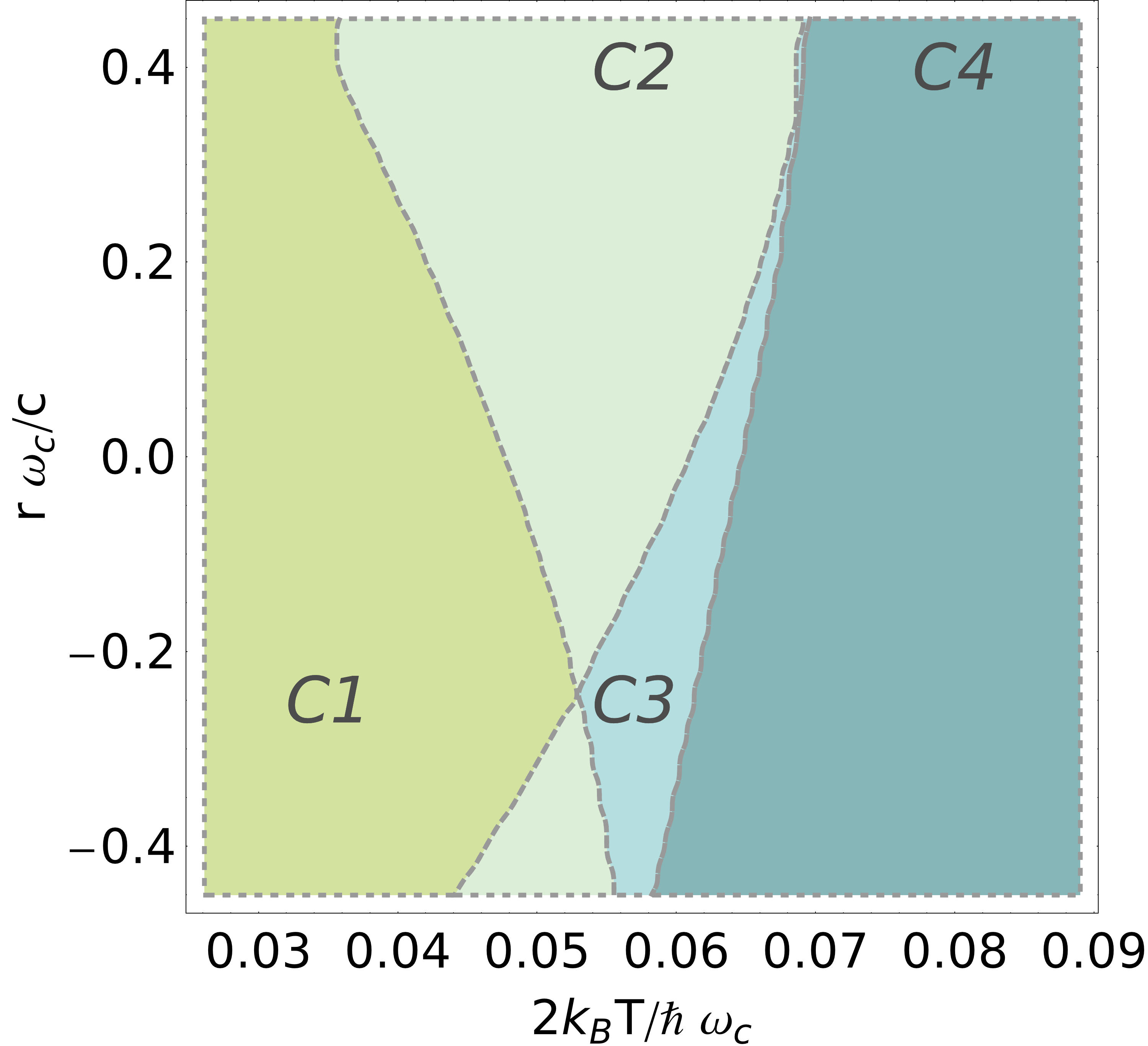
Figure 5: (Color online) Phase diagram of the separability classes for the linear configuration as function of temperature and the position $r$ of oscillator $\mathcal{B}$. All other parameters are as in Fig. 3.

Concerning tripartite entanglement a most important question is whether an optimal arrangement for genuine tripartite entanglement exits. The results of the previous section suggest that equally spaced oscillators might be rather unfavorable for two-mode entanglement (see inset in Fig. 3). An expectation inferred from those results (see Fig. 2) is that tripartite entanglement decreases with distance as bipartite entanglement does, i.e., it should vanish at large distances. Still it is interesting to see whether three-mode entanglement is more robust against variation of $r$ than two-mode entanglement. Moreover, the limiting distance may be different from $R\omega_{c}/c$.

III.3.1 Linear arrangement

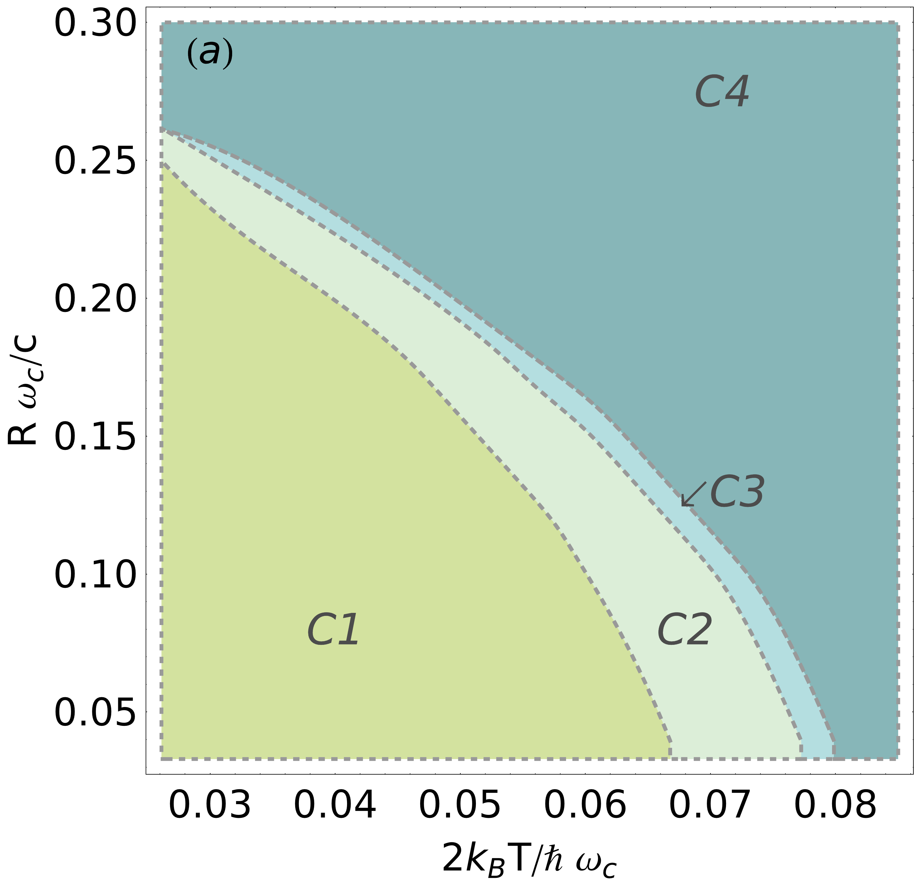
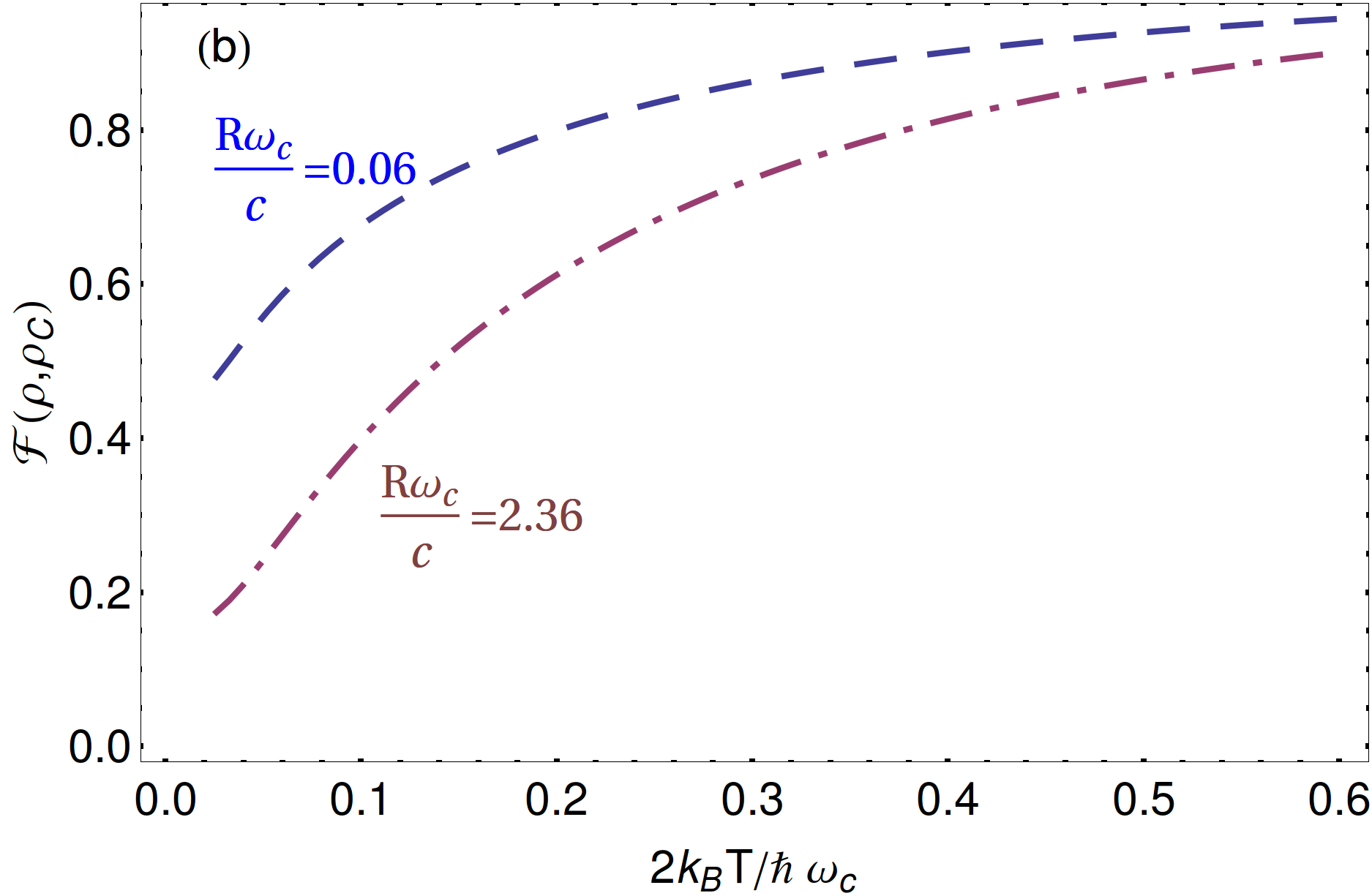
Figure 6: (Color online) (a) Separability phase diagram for the equilateral-triangular for the oscillator frequencies and coupling strengths used in Fig. 4. (b) Quantum fidelity between the stationary state and the thermal canonical state as a function of the temperature for the distances $R\omega_{c}/c=0.066$ (blue-dashed line) and $R\omega_{c}/c=2.367$ (pink-dot-dashed line).

Figure 5 shows the phase diagram of the separability classes for the case in which all oscillators are coupled to a one-dimensional environment. Most importantly, it demonstrates the relative robustness of the fully inseparable states (class C1) against shifting the position of oscillator $\mathcal{B}$ and against moderate temperature increase. Fully inseparable states are found for small temperatures and when oscillator $\mathcal{B}$ is a bit closer to $\mathcal{A}$ than to $\mathcal{C}$. This asymmetry stems from the fact that the oscillator $\mathcal{C}$ is less affected by the thermal fluctuations than the other two oscillators, owing to its larger frequency. In general, we expect the genuine tripartite entanglement to be rather insensitive to variations of the geometry as long as all oscillators interact strongly in the same manner through the reservoir, i.e., when oscillator $\mathcal{B}$ is roughly in the middle. Otherwise, the geometry could enhance the interaction between two particular oscillators, which may lead to a situation in which the third oscillator becomes separable. In the phase diagram (Fig. 5), this is visible in the emergence of regions with separability class C2 when $r$ tends towards $\pm R/2$. Thus, in contrast to the two-mode case, the equidistant placement of oscillator $\mathcal{B}$ at $r=0$ is the optimal setting for genuine tripartite entanglement, at least in the case of equal oscillators.

III.3.2 Arrangement in an equilateral triangle

Having noticed that in the 1D case, optimal tripartite entanglement is achieved in the most symmetric situation, we restrict ourselves in the 3D case to the configuration in an equilateral triangle with lateral length $R=\Delta\bm{r}^{0}_{\mathcal{A}\mathcal{C}}=\Delta\bm{r}^{0}_{\mathcal{B}\mathcal{C}}=\Delta\bm{r}^{0}_{\mathcal{A}\mathcal{B}}$. Figure 6(a) depicts the corresponding separability phase diagram. Again we find for small $R$ and low temperatures that the stationary state is fully inseparable (class C1). With increasing temperature, we notice a transition via the one-, two-, and three-mode biseparable classes C2, C3, and C4 to the fully separable class C5 at high temperatures $T\gtrsim\hbar\omega_{c}/k_{B}$ (the latter is beyond the plotted range). The appearance of classes C2 and C3 obviously requires some asymmetry in the setup, which stems from choosing different oscillator frequencies. In comparison to the two-mode entanglement studied in Sec. III.1, however, tripartite bound entanglement (class C4) is more robust against separation and temperature effects than for two modes. Indeed we find that it may survive up to values of $R\omega_{c}/c$ that clearly exceed unity. This can be explained by the fact that the susceptibilities reflect an effective coupling of all oscillators independent of their spatial separation (cf. discussion in the Sec. II.2), which enables large-distance entanglement. The latter is also in agreement with the two-mode entanglement $E_{N}(\rho_{\mathcal{A}\mathcal{C}})$ discussed above: It asymptotically approaches the value found for the oscillator pair $\mathcal{A}\mathcal{C}$ in the absence of a third oscillator (see inset of Fig. 4) and underlines that the environment induces long-range interaction. On the other hand, the quantum fidelity (28), which shows the “sophistication” of the stationary state, reveals that the (fully separable) thermal state is reached for $k_{B}T/\hbar\omega_{c}\gtrsim 1$ [see Fig. 6(b)], irrespective of the distances between the oscillators. Hence, only at high temperatures, decoherence dominates so that here the full separability turns out to be a decoherence phenomenon.

IV Summary and Conclusions

We have studied the dynamics of three harmonic oscillators as a generic tripartite system that becomes entangled through the interaction with a common extended environment. The oscillators are embedded in a thermal bosonic heat bath which we eliminated to obtain generalized quantum Langevin equations. Although the oscillators are not directly coupled, the contact via the heat bath provides an environment-mediated interaction which can induce bipartite and tripartite entanglement among the oscillators. The equations of motion for a 1D and 3D isotropic environment contain this interaction as a long-range coupling entering via a renormalization term and through the susceptibility, which takes the backaction into account. For both two-mode entangled and fully inseparable oscillators, the characteristic correlation length is roughly given by the ratio $R\omega_{c}/c$. For a 3D environment it is smaller than for the 1D case. Nevertheless, the entanglement generated by a 3D environment is more robust against thermal fluctuations. As expected, non-Markovian memory effects play a crucial role for the dynamics. Interestingly enough, there is a trade-off in the attainable two-mode entanglement between the different oscillator pairs, because the presence of a passive oscillator is detrimental for two-mode entanglement. This provides strong evidence that the environment-induced interaction is mainly a many-parties interaction that tends to favor multi-partite correlations (here tripartite instead of bipartite), such that GHZ-like states emerge. In general, the numerical data suggest that the mechanism is based on uncontrolled feedback which is mostly coherent at low temperatures and for moderate oscillator-environment coupling (in comparison to the fundamental frequencies).

Our findings underline that non-Markovian effects are the key towards a deeper understanding of this kind of entanglement dynamics. This is in contrast to the behavior of subsystems coupled to independent heat baths, for which non-Markovian effects are not essential, while thermal relaxation and decoherence-free subspaces dominate. An interesting consequence of our results in the realm of quantum information may be found in setups for quantum communication and teleportation. Considering the studied model as a simplified quantum network, our result for two-mode entanglement in the presence of a passive oscillator imply the need for sufficient microscopic control of the interaction between all constituents. Thus, an interesting task would be the prediction of the stability of such protocols under even weak interaction with a common extended environment.

Appendix A The system-environment model

In this appendix we derive the Langevin equation and different quantities used in the main text. We start with the Hamiltonians $H_{S}$, $H_{B}$, and $H_{I}$, Eqs. (3) and (5). We shall first neglect the counter-term (renormalization) whose contribution will be included at the end. Hence, the Hamiltonian equations of motion for $p_{\lambda}$ and $a_{\bm{k}}$ are given by

$$\dot{p}_{\lambda} = -m\omega_{\lambda}^{2}x_{\lambda}+\sum_{k}g_{\bm{k}}\left(a_{\bm{k}}e^{i\bm{k}\cdot\bm{r}^{0}_{\lambda}}+a^{\dagger}_{\bm{k}}e^{-i\bm{k}\cdot\bm{r}^{0}_{\lambda}}\right),$$ (33)

$$\dot{a}_{\bm{k}} = -i\omega_{\bm{k}}a_{\bm{k}}{+}\frac{i}{\hbar}\sum_{\mu}g_{\bm{k}}e^{-i\bm{k}\cdot\bm{r}^{0}_{\mu}}x_{\mu},$$ (34)

where the latter possesses the formal solution

$$a_{\bm{k}}(t) = a_{\bm{k}}(t_{0})e^{-i\omega_{\bm{k}}(t-t_{0})}{+}$$

$$+ \frac{i}{\hbar}\sum_{\mu}g_{\bm{k}}e^{-i\bm{k}\cdot\bm{r}^{0}_{\mu}}\int_{t_{0}}^{t}dsx_{\mu}(s)e^{-i\omega_{\bm{k}}(t-s)}.$$

We insert it into Eq. (33) to obtain for the oscillators conditioned to the state of the environment the effective dynamical equation

$$\begin{split}\dot{p}_{\lambda}={}&-m\omega_{\lambda}^{2}x_{\lambda}+F_{\lambda}(t)\\ &+\frac{i}{\hbar}\sum_{\mu}\sum_{\bm{k}}g_{\bm{k}}^{2}e^{i\bm{k}\cdot\left(\bm{r}^{0}_{\lambda}-\bm{r}^{0}_{\mu}\right)}\int_{t_{0}}^{t}dsx_{\mu}(s)e^{-i\omega_{\bm{k}}(t-s)}\\ &-\frac{i}{\hbar}\sum_{\mu}\sum_{\bm{k}}g_{\bm{k}}^{2}e^{-i\bm{k}\cdot\left(\bm{r}^{0}_{\lambda}-\bm{r}^{0}_{\mu}\right)}\int_{t_{0}}^{t}dsx_{\mu}(s)e^{i\omega_{\bm{k}}(t-s)}.\end{split}$$ (35)

This equation can be expressed in a more convenient form by introducing the fluctuating force $F_{\lambda}(t)$ and susceptibility $\chi_{\lambda\mu}(t)$ to read

$$\dot{p}_{\lambda}(t)+m\omega_{\lambda}^{2}x_{\lambda}+\frac{1}{\hbar}{\displaystyle\int_{t_{0}}^{t}}d\tau\sum_{\mu}\chi_{\lambda\mu}(t-\tau)x_{\mu}(\tau)=F_{\lambda}(t),$$

where

$$F_{\lambda}(t) = \sum_{\bm{k}}g_{\bm{k}}\Big{(}a_{\bm{k}}(t_{0})e^{i(\bm{k}\cdot\bm{r}^{0}_{\lambda}-\omega_{\bm{k}}(t-t_{0}))}$$

$$\qquad+a_{\bm{k}}^{\dagger}(t_{0})e^{-i(\bm{k}\cdot\bm{r}^{0}_{\lambda}-\omega_{\bm{k}}(t-t_{0}))}\Big{)},$$

$$\chi_{\lambda\mu}(t) = 2\Theta\left(t-|\Delta\bm{r}^{0}_{\lambda\mu}|/c\right)\sum_{\bm{k}}g_{\bm{k}}^{2}\sin\left(\bm{k}\cdot\Delta\bm{r}^{0}_{\lambda\mu}-\omega_{\bm{k}}t\right).$$

The susceptibility can be written in terms of an average over the environmental state $\rho_{B}$ of the commutator of the fluctuating force, so that it becomes

$$\chi_{\lambda\mu}\left(t-t^{\prime}\right)=-i\Theta(t-t^{\prime}-|\Delta\bm{r}^{0}_{\lambda\mu}|/c)\big{\langle}\left[F_{\lambda}(t),F_{\mu}(t^{\prime})\right]\big{\rangle}_{\rho_{B}},$$ (36)

where $|\Delta\bm{r}^{0}_{\lambda\mu}|=|\bm{r}^{0}_{\lambda}-\bm{r}^{0}_{\mu}|$.

The environment is initially in an equilibrium state at temperature $T$ for which $\langle a^{\dagger}_{\bm{k}^{\prime}}a_{\bm{k}}\rangle=\delta_{\bm{k}\bm{k}^{\prime}}N(\omega_{\bm{k}})$, with the bosonic thermal occupation $N(\omega_{\bm{k}})=[\exp(-\omega_{\bm{k}}/k_{B}T)-1]^{-1}$ so that the anti-commutator of the fluctuating force obeys

$$\begin{split}\big{\langle}\left\{F_{\lambda}(t),F_{\mu}(t^{\prime})\right\}\big{\rangle}_{\rho_{B}}={}&2\sum_{\bm{k}}g_{\bm{k}}^{2}{\Big{(}2N(\omega_{\bm{k}})+1\Big{)}}\\ &\times\cos\left[\bm{k}\cdot\Delta\bm{r}^{0}_{\lambda\mu}-\omega_{\bm{k}}(t-t^{\prime})\right].\end{split}$$ (37)

In the frequency domain, this relation reads

$$\begin{split}\big{\langle}\{F_{\lambda}(\omega),F_{\mu}(\omega^{\prime})\}\big{\rangle}_{\rho_{B}}={}&4\pi^{2}\delta\left(\omega^{\prime}+\omega\right)\coth\left(\frac{\hbar\omega^{\prime}}{2k_{B}T}\right)\\ &\times\sum_{\bm{k}}g_{\bm{k}}^{2}\Big{(}e^{ik\Delta x_{\lambda\mu}}\delta\left(\omega^{\prime}-\omega_{\bm{k}}\right)\\ &-e^{-ik\Delta x_{\lambda\mu}}\delta\left(\omega^{\prime}+\omega_{\bm{k}}\right)\Big{)},\end{split}$$ (38)

where we have inserted $2N(\omega_{\bm{k}})+1=\coth\left(\hbar\omega/2K_{B}T\right)$. For a more compact notation, we introduce the spectral densities

$$J_{\lambda{,}\mu}(\omega)=\frac{\pi}{\hbar}\sum_{\bm{k}}g_{\bm{k}}^{2}\cos\left(\bm{k}\cdot\Delta\bm{r}^{0}_{\lambda\mu}\right)\delta\left(\omega-\omega_{\bm{k}}\right),$$ (39)

with which we obtain from Eq. (38) the quantum fluctuation-dissipation relation

$$\mathop{\mathrm{Re}}\frac{1}{2}{\Big{\langle}\left\{{F_{\lambda}(\omega),F_{\mu}(\omega^{\prime})}\right\}\Big{\rangle}}=2\pi\hbar\delta\left(\omega^{\prime}+\omega\right)\Gamma_{\lambda\mu}(\omega^{\prime}),$$ (40)

with the imaginary part of the susceptibility

$$\Gamma_{\lambda\mu}(\omega)={} -\frac{1}{\hbar}\hbox{Im }\chi_{\lambda\mu}(\omega){\coth\left(\frac{\hbar\omega^{\prime}}{2K_{B}T}\right)}$$ (41)

$$={} J_{\lambda,\mu}(|\omega|)\,{\coth\left(\frac{\hbar|\omega|}{2K_{B}T}\right)},$$

derived in Appendix B.

So far we have not taken into account the counter-term. In doing so, the spectral densities lead to harmonic renormalization potentials with frequencies

$$\tilde{\Omega}_{\lambda\lambda} = \frac{1}{\hbar}\sum_{\bm{k}}\frac{g_{\bm{k}}^{2}}{\omega_{\bm{k}}}=\frac{1}{\pi}\int_{0}^{\infty}\frac{J_{\lambda,\lambda}(\omega)}{\omega}d\omega,$$ (42)

$$\tilde{\Omega}_{\lambda\mu} = \frac{1}{\hbar}\sum_{\bm{k}}\frac{g_{\bm{k}}^{2}}{\omega_{\bm{k}}}\cos\left(\bm{k}\cdot\Delta\bm{r}^{0}_{\lambda\mu}\right)=\frac{1}{\pi}\int_{0}^{\infty}\frac{J_{\lambda,\mu}(\omega)}{\omega}d\omega.$$

Owing to the linearity of the dynamical equations for $x_{\lambda}$ and $p_{\lambda}$, it is straightforward to show that including the counter-term provides the Langevin equation (7).

Appendix B Spectral densities and susceptibilities

Irrespective of the dimension of the environment, we assume that it is isotropic and possesses the linear dispersion relation $\omega_{\bm{k}}=c|\bm{k}|$ with cut-off frequency $\omega_{c}$. We model this by introducing coupling constants $g_{\bm{k}}$ that obey

$$g^{2}_{\bm{k}}=m\hbar\gamma(\omega_{\bm{k}}/\omega_{c}^{d-1})c^{d}V_{\bm{k}}(d)e^{-\omega/\omega_{c}},$$ (43)

where $d$ is the dimension of the environment, $V_{\bm{k}}$ is the $d$-dimensional $\bm{k}$-space volume per field mode, and $\gamma$ is the effective coupling strength. We start from Eq. (39) and take the continuum limit $V_{\bm{k}}\to 0$. We provide explicit expressions for the dimensions $d=1$ and $d=3$, while $d=2$ is addressed mainly for highlighting the difficulties that arise in that dimension.

B.1 One-dimensional environment

Inserting Eq. (43) for $d=1$ into (39) and (42) yields in the continuum limit $V_{\bm{k}}(1)\rightarrow 0$ for the spectral density the closed-form form

$$J_{\lambda\mu}(\omega)=\pi m\gamma\omega e^{-\omega/\omega_{c}}\cos(\omega|\Delta\bm{r}^{0}_{\lambda\mu}|/c),$$ (44)

and the potential renormalization frequencies

$$\tilde{\Omega}_{\lambda\lambda} = m\gamma\omega_{c},$$

$$\tilde{\Omega}_{\lambda\mu} = \frac{m\gamma\omega_{c}}{1+(\omega_{c}|\Delta\bm{r}^{0}_{\lambda\mu}|/c)^{2}},$$

respectively. The real part of the susceptibility ${\chi_{\lambda\mu}(\omega^{\prime})}$ is obtained from Eq. (41) via the Kramers-Kronig relations. Mathematically this corresponds to the Hilbert transformation erdelyi1954 can formally be expressed as

$$\begin{split}\mathop{\mathrm{Re}}{\chi_{\lambda\mu}(\omega^{\prime})}={}&\mathcal{H}\left[\mathop{\mathrm{Im}}\chi_{\lambda\mu}(\omega)\right]\left(\omega^{\prime}\right)\\ :={}&\frac{1}{\pi}P\int_{-\infty}^{\infty}\frac{\mathop{\mathrm{Im}}\chi_{\lambda\mu}(\omega)}{\omega-\omega^{\prime}}d\omega,\end{split}$$ (45)

where $P$ is the Cauchy principal value and $\mathcal{H}[f(\omega)](\omega^{\prime})$ the Hilbert transform of $f(\omega)$. Hence,

$$\begin{split}\mathop{\mathrm{Re}}{\chi_{\lambda\mu}(\omega)}={}&-m\hbar\gamma P\int_{0}^{\infty}\omega e^{-\omega/\omega_{c}}\cos(\omega|\Delta\bm{r}^{0}_{\lambda\mu}|/c)\\ &\times\Big{(}\frac{1}{\omega-\omega^{\prime}}+\frac{1}{\omega+\omega^{\prime}}\Big{)}d\omega,\end{split}$$ (46)

which consists of two terms that differ by the sign of $\omega^{\prime}$ and, thus, it is sufficient to compute

$$P\int_{0}^{\infty}\frac{\omega e^{-\omega/\omega_{c}}\cos(\omega|\Delta\bm{r}^{0}_{\lambda\mu}|/c)}{\omega-\omega^{\prime}}d\omega=\omega^{\prime}P\int_{0}^{\infty}\frac{e^{-\omega/\omega_{c}}\cos(\omega|\Delta\bm{r}^{0}_{\lambda\mu}|/c)}{\omega-\omega^{\prime}}d\omega+\frac{\omega_{c}}{1+(\omega_{c}|\Delta\bm{r}^{0}_{\lambda\mu}|/c)^{2}},$$

where we have used $\mathcal{H}[\omega f(\omega)]=\omega\mathcal{H}(f(\omega))+\frac{1}{\pi}\int_{-\infty}^{\infty}f(\omega)d\omega$ to arrive at

$$P\int_{0}^{\infty}\frac{e^{-\left(\frac{1}{\omega_{c}}-i|\Delta\bm{r}^{0}_{\lambda\mu}|/c\right)\omega}}{\omega-\omega^{\prime}}d\omega=\begin{cases}{e^{-\left(\frac{1}{\omega_{c}}-i|\Delta\bm{r}^{0}_{\lambda\mu}|/c\right)\omega^{\prime}}\left\{\Gamma\left[0,-\left(\frac{1}{\omega_{c}}-i|\Delta\bm{r}^{0}_{\lambda\mu}|/c\right)\omega^{\prime}\right]+i\pi\right\}}&\mbox{if }\,\omega^{\prime}\,\in(0,\infty)\\ {e^{-\left(\frac{1}{\omega_{c}}-i|\Delta\bm{r}^{0}_{\lambda\mu}|/c\right)\omega^{\prime}}\Gamma\left[0,-\left(\frac{1}{\omega_{c}}-i|\Delta\bm{r}^{0}_{\lambda\mu}|/c\right)\omega^{\prime}\right]}&\mbox{if }\,\omega^{\prime}\,\in(-\infty,0).\end{cases}$$

where $\Gamma(a,z)=\int^{z}_{\infty}t^{a-1}e^{-t}dt$ denotes the incomplete gamma function. Inserting this expression into Eq. (46), we finally obtain

$$\mathop{\mathrm{Re}}{\chi_{\lambda\mu}(\omega)} = -m\hbar\gamma\omega\mathop{\mathrm{Re}}\left[g(\omega)-g(-\omega)\right]+\pi m\hbar\,\gamma\,\omega\,\mathop{\mathrm{Im}}\big{[}\Theta\left(\omega\right)e^{-\left(\frac{1}{\omega_{c}}-i|\Delta\bm{r}^{0}_{\lambda\mu}|/c\right)\omega}$$ (47)

$$-\Theta\left(-\omega\big{]}e^{\left(\frac{1}{\omega_{c}}-i|\Delta\bm{r}^{0}_{\lambda\mu}|/c\right)\omega}\right)-\frac{2m\hbar\gamma\omega_{c}}{1+(\omega_{c}|\Delta\bm{r}^{0}_{\lambda\mu}|/c)^{2}},$$

with $g(\omega)=e^{-(1-i\omega_{c}|\Delta\bm{r}^{0}_{\lambda\mu}|/c)\omega/\omega_{c}}\Gamma[0,-(1-i\omega_{c}|\Delta\bm{r}^{0}_{\lambda\mu}|/c)\omega/\omega_{c}]$. From this expression we find the well known relation between the frequency shift $\Delta\omega_{\lambda\mu}$ and the real part of susceptibility riseborough19851 ,

$$\left(\Delta\omega_{\lambda\mu}\right)^{2}=-\frac{\tilde{\Omega}_{\lambda\mu}}{m}=\frac{1}{2m\hbar}\lim_{\omega\rightarrow 0}\mathop{\mathrm{Re}}{\chi_{\lambda\mu}(\omega)}.$$

B.2 Two-dimensional environment

Again, we use (43), perform the continuum limit, and readily obtain

$$J_{\lambda\mu}(\omega)=2\pi^{2}m\gamma\frac{\omega^{2}}{\omega_{c}}e^{-\omega/\omega_{c}}\mathsf{J}_{0}(\omega|\Delta\bm{r}^{0}_{\lambda\mu}|/c),$$ (48)

where $\mathsf{J}_{0}$ is the zeroth-order Bessel function of the first kind. The renormalization frequencies now become

$$\tilde{\Omega}_{\lambda\lambda} = 2\pi m\gamma\omega_{c},$$

$$\tilde{\Omega}_{\lambda\lambda^{\prime}} = \frac{2\pi m\gamma\omega_{c}}{[1+(\omega_{c}|\Delta\bm{r}^{0}_{\lambda\mu}|/c)^{2}]^{3/2}}.$$

Accordingly, the Fourier transform of the real part of the susceptibility reads

$$\begin{split}\mathop{\mathrm{Re}}\chi_{\lambda\mu}(\omega^{\prime})={}&-\frac{2\pi m\gamma\hbar}{\omega_{c}}P\int_{0}^{\infty}\omega^{2}e^{-\omega/\omega_{c}}\mathsf{J}_{0}(\omega|\Delta\bm{r}^{0}_{\lambda\mu}|/c)\\ &\times\left(\frac{1}{\omega-\omega^{\prime}}+\frac{1}{\omega+\omega^{\prime}}\right)d\omega.\end{split}$$ (49)

Using the same relation of Hilbert transforms as in the previous section we can write,

$$\begin{split}\mathcal{H}[&\Theta(\omega)\omega^{2}e^{-\omega/\omega_{c}}\mathsf{J}_{0}(\omega|\Delta\bm{r}^{0}_{\lambda\mu}|/c)](\omega^{\prime})\\ ={}&\omega^{\prime 2}\mathcal{H}[\Theta(\omega)e^{-\omega/\omega_{c}}\mathsf{J}_{0}(\omega|\Delta\bm{r}^{0}_{\lambda\mu}|/c)](\omega^{\prime})\\ &+\frac{\omega^{\prime}\omega_{c}}{[1+(\omega_{c}|\Delta\bm{r}^{0}_{\lambda\mu}|/c)^{2}]^{1/2}}+\frac{\omega_{c}^{2}}{[1+(\omega_{c}|\Delta\bm{r}^{0}_{\lambda\mu}|/c)^{2}]^{3/2}}.\end{split}$$

Here a major difficulty arises. The Hilbert transform $\mathcal{H}[\Theta(\omega)e^{-\omega/\omega_{c}}\mathsf{J}_{0}({\omega|\Delta\bm{r}^{0}_{\lambda\mu}|}/{c})](\omega^{\prime})$ exists only for $R/c=1$, despite the convergence condition $0<\omega_{c}$. Thus, we cannot derive any closed expression for $\mathop{\mathrm{Re}}\chi(\omega)$ for all $R$ and $c$. Still we obtain by using a series representation for $\mathsf{J}_{0}({\omega|\Delta\bm{r}^{0}_{\lambda\mu}|}/{c})$ the relation

$$\begin{split}\mathop{\mathrm{Re}}{\chi(\omega)}={}&\frac{2\pi m\gamma\hbar}{\omega_{c}}\omega^{2}\Big{[}\Theta(\omega)e^{\frac{-\omega}{\omega_{c}}}Ei\left(\frac{\omega}{\omega_{c}}\right)\\ &-\Theta(-\omega)e^{\frac{\omega}{\omega_{c}}}Ei\left(\frac{-\omega}{\omega_{c}}\right)\Big{]}\mathsf{J}_{0}({{|\Delta\bm{r}^{0}_{\lambda\mu}|}\omega}/{c})\\ &-2\pi m\gamma\hbar\omega_{c}\sum_{l=0}^{\infty}\frac{(-1)^{l}}{2^{2l}}\left(\frac{{|\Delta\bm{r}^{0}_{\lambda\mu}|}\omega_{c}}{c}\right)^{2l}\\ &\times\sum_{k=1}^{l+1}\frac{(2(l-k)+3)!}{l!l!}\left(\frac{\omega}{\omega_{c}}\right)^{2(k-1)}.\end{split}$$ (50)

This series, however, it is not of practical use, because of its slow convergence.

B.3 Three-dimensional environment

Following once more the same line, we obtain the spectral densities

$$J_{\lambda\mu}(\omega)=4\pi^{2}m\gamma\frac{c}{|\Delta\bm{r}^{0}_{\lambda\mu}|}\Big{(}\frac{\omega}{\omega_{c}}\Big{)}^{2}\sin(\omega|\Delta\bm{r}^{0}_{\lambda\mu}|/c)e^{-\omega/\omega_{c}},$$ (51)

and the renormalization frequencies

$$\tilde{\Omega}_{\lambda\lambda} = 8\pi m\gamma\omega_{c}$$

$$\tilde{\Omega}_{\lambda\mu} = \frac{8\pi m\gamma\omega_{c}}{[1+(\omega_{c}|\Delta\bm{r}^{0}_{\lambda\mu}|/c)^{2}]^{2}}.$$

Now the real part of the susceptibility is given by

$$\begin{split}\mathop{\mathrm{Re}}{\chi_{\lambda\mu}(\omega^{\prime})}={}&-\frac{4\pi m\hbar\gamma}{\omega_{c}^{2}}\Big{(}\frac{c}{|\Delta\bm{r}^{0}_{\lambda\mu}|}\Big{)}P\int_{0}^{\infty}\sin(\omega|\Delta\bm{r}^{0}_{\lambda\mu}|/c)\\ &\times\omega^{2}e^{-\omega/\omega_{c}}\Big{(}\frac{1}{\omega-\omega^{\prime}}+\frac{1}{\omega+\omega^{\prime}}\Big{)}d\omega,\end{split}$$ (52)

where the integral can be written as

$$\begin{split}{\frac{1}{\pi}}P&\int_{0}^{\infty}\frac{\omega^{2}\sin(\omega|\Delta\bm{r}^{0}_{\lambda\mu}|/c)e^{\frac{-\omega}{\omega_{c}}}}{\omega-\omega^{\prime}}d\omega\\ ={}&\omega^{\prime 2}\mathcal{H}\left[\Theta(\omega)\sin(\omega|\Delta\bm{r}^{0}_{\lambda\mu}|/c)e^{\frac{-\omega}{\omega_{c}}}\right](\omega^{\prime})\\ &+{\frac{\omega^{\prime}}{\pi}}\frac{\omega_{c}^{2}|\Delta\bm{r}^{0}_{\lambda\mu}|/c}{[1+(\omega_{c}|\Delta\bm{r}^{0}_{\lambda\mu}|/c)^{2}]}\\ &+{\frac{1}{\pi}}\frac{2\omega_{c}^{3}|\Delta\bm{r}^{0}_{\lambda\mu}|/c}{[1+(\omega_{c}|\Delta\bm{r}^{0}_{\lambda\mu}|/c)^{2}]^{2}}.\end{split}$$ (53)

After some algebra, we finally obtain for the real part of the 3D-susceptibility the expression

$$\begin{split}\mathop{\mathrm{Re}}{\chi_{\lambda\nu}(\omega)}={}&{-\frac{4\pi m\hbar\gamma c\omega^{2}}{\omega_{c}^{2}{|\Delta\bm{r}^{0}_{\lambda\mu}|}}\mathop{\mathrm{Im}}\left[g(\omega)+g(-\omega)\right]}\\ &-\frac{4\pi^{2}m\hbar\gamma c\omega^{2}}{\omega_{c}^{2}{|\Delta\bm{r}^{0}_{\lambda\mu}|}}\mathop{\mathrm{Re}}\big{[}\Theta(\omega)e^{-(\frac{1}{\omega_{c}}-i|\Delta\bm{r}^{0}_{\lambda\mu}|/c)\omega}\\ &+\Theta(-\omega)e^{(\frac{1}{\omega_{c}}-i|\Delta\bm{r}^{0}_{\lambda\mu}|/c)\omega}\big{]}\\ &-\frac{16\pi m\hbar\gamma\omega_{c}}{[1+(\omega_{c}|\Delta\bm{r}^{0}_{\lambda\mu}|/c)^{2}]^{2}}\end{split}$$ (54)

with $g(\omega)=e^{-(1-i\omega_{c}|\Delta\bm{r}^{0}_{\lambda\mu}|/c)\omega/\omega_{c}}\Gamma[0,-(1-i\omega_{c}|\Delta\bm{r}^{0}_{\lambda\mu}|/c)\omega/\omega_{c}]$ and the incomplete gamma function $\Gamma(0,x)$.

Appendix C Fourier representation of Eq. (38)

Here a give a simple proof of Eq. (41) starting from the Fourier transform of the susceptibility

$$\chi_{\lambda\mu}\left(\omega\right) = \int_{-\infty}^{\infty}e^{i\omega t}\chi_{\lambda\mu}(t)\,dt$$

$$= 2\int\limits_{|\Delta\bm{r}^{0}_{\lambda\mu}|/c}^{\infty}e^{i\omega t}\sum_{\bm{k}}g_{\bm{k}}^{2}\sin\left(\bm{k}\cdot\Delta\bm{r}^{0}_{\lambda\mu}-\omega_{\bm{k}}t\right)\,dt$$

$$= -i\sum_{\bm{k}}g_{\bm{k}}^{2}\Bigg{[}e^{i\left(\bm{k}\cdot\Delta\bm{r}^{0}_{\lambda\mu}-\left(\omega-\omega_{\bm{k}}\right)|\Delta\bm{r}^{0}_{\lambda\mu}|/c\right)}$$

$$\times\int\limits_{0}^{\infty}e^{i\left(\omega-\omega_{\bm{k}}\right)t}\,dt-e^{-i\left(\bm{k}\cdot\Delta\bm{r}^{0}_{\lambda\mu}-\left(\omega+\omega_{\bm{k}}\right)|\Delta\bm{r}^{0}_{\lambda\mu}|/c\right)}$$

$$\times\int\limits_{0}^{\infty}e^{i\left(\omega+\omega_{\bm{k}}\right)t}\,dt\Bigg{]},$$

where we have made the substitution $t\to t+|\Delta\bm{r}^{0}_{\lambda\mu}|/c$. Inserting

$$\int_{0}^{\infty}e^{i\left(\omega-\omega_{\bm{k}}\right)t}\,dt=\pi\delta\left(\omega-\omega_{\bm{k}}\right)+i\mathcal{H}\left(1\right)\left(\omega_{\bm{k}}\right)$$

into Eq. (C) yields

$$\begin{split}\chi_{\lambda\mu}\left(\omega\right)={}&-i\pi\sum_{\bm{k}}g_{\bm{k}}^{2}\Big{\{}e^{i\left(\bm{k}\cdot\Delta\bm{r}^{0}_{\lambda\mu}-\left(\omega-\omega_{\bm{k}}\right)|\Delta\bm{r}^{0}_{\lambda\mu}|/c\right)}\\ &\times\delta(\omega-\omega_{\bm{k}})-e^{-i(\bm{k}\cdot\Delta\bm{r}^{0}_{\lambda\mu}-(\omega+\omega_{\bm{k}})|\Delta\bm{r}^{0}_{\lambda\mu}|/c)}\\ &\times\delta(\omega+\omega_{\bm{k}})\Big{\}}\\ &+\sum_{\bm{k}}g_{\bm{k}}^{2}\Big{\{}e^{i\left(\bm{k}\cdot\Delta\bm{r}^{0}_{\lambda\mu}-\left(\omega-\omega_{\bm{k}}\right)|\Delta\bm{r}^{0}_{\lambda\mu}|/c\right)}\mathcal{H}(1)\left(\omega_{\bm{k}}\right)\\ &-e^{-i\left(\bm{k}\cdot\Delta\bm{r}^{0}_{\lambda\mu}-\left(\omega+\omega_{\bm{k}}\right)|\Delta\bm{r}^{0}_{\lambda\mu}|/c\right)}\mathcal{H}\left(1\right)\left(\omega_{\bm{k}}\right)\Big{\}},\end{split}$$

where the second sum vanishes owing to $\mathcal{H}(1)(\omega_{\bm{k}})=0$ erdelyi1954 . By taking the imaginary part and performing the continuum limit, we obtain Eq. (41).

Appendix D PPT criterion and classification of tripartite entanglement

Let us consider a system composed of two parties $A$ and $B$. Then a necessary and sufficient condition for the separability between $1_{A}\times 1_{B}$ (two modes), $1_{A}\times N_{B}$, and $N_{A}\times N_{B}$ bisymmetric bipartite states is the partial positive transpose (PPT) criterion adesso20071 ; serafini20051 . The $N_{A}\times N_{B}$ class of systems relates to Gaussian states that are locally invariant under all permutations of modes in each of the two subsystems. Then the PPT criterion can be formulated in terms of a bisymmetric covariance matrix ${G}$ as follows: A state is separable if and only if ${G}^{T_{B}}\geq({i}\hbar/{2}){\sigma}$ (i.e., ${G}^{T_{B}}$ is a positive-definite matrix), where ${G}^{T_{B}}$ is the covariance matrix of the partial transpose of ${G}$ with respect to the system $B$, given by ${G}^{T_{B}}=:{\Lambda}{G}{\Lambda},$ with

$${\Lambda}=\mathbb{I}_{N_{A}+N_{B}}\oplus\begin{bmatrix}\mathbb{I}_{N_{A}}&0\\ 0&-\mathbb{I}_{N_{B}}\\ \end{bmatrix},$$

the $N$-dimensional unit matrix $\mathbb{I}_{N}$, and the symplectic matrix

$${\sigma}=\begin{bmatrix}0&\mathbb{I}_{N_{A}+N_{B}}\\ -\mathbb{I}_{N_{A}+N_{B}}.&0\\ \end{bmatrix}\,.$$

The PPT criterion can readily be evaluated from the symplectic eigenvalues of ${G}^{T_{B}}$, given by the positive square roots of the eigenvalues of $(-i/\hbar){\sigma}{G}^{T_{B}}$ vidal20021 .

For a system composed of three-modes, Giedke et al. giedke20011 have considered the PPT criterion to provide a complete classification of the three-mode states, according their separability properties. This classification is based on the partially transposed covariance matrices $\tilde{{G}}^{T_{\lambda}}={\Lambda}_{\lambda}{G}{\Lambda}_{\lambda}$, which is related to the three possible bi-partitions of a three-component system, namely $\mathcal{A}|\mathcal{B}\mathcal{C}$, $\mathcal{A}\mathcal{B}|\mathcal{C}$ and $\mathcal{A}\mathcal{C}|\mathcal{B}$. Then each three-mode Gaussian state can be assigned to one of the following classes giedke20011 :

1. Fully inseparable states that are not separable under any of the three possible bipartitions. This class contains the genuine tripartite entangled states benatti20111 .

2. One-mode biseparable states that are separable if two of the parties are grouped together, but inseparable with respect to the other groupings.

3. Two-mode biseparable states for which two of the bipartitions are separable.

4. Three-mode biseparable states for which all the three bipartitions are separable, but which cannot be written as a mixture of tripartite product states. These states are also known as tripartite bound entangled states.

5. Fully separable states that can be written as a mixture of tripartite product states.

References

• (1) R. Horodecki, P. Horodecki, M. Horodecki, and K. Horodecki, Rev. Mod. Phys. 81, 865 (2009).
• (2) W. H. Zurek, Rev. Mod. Phys. 75, 715 (2003).
• (3) D. Braun, Phys. Rev. Lett. 89, 277901 (2002).
• (4) M. B. Plenio and S. F. Huelga, Phys. Rev. Lett. 88, 197901 (2002)
• (5) F. Benatti, R. Floreanini, and M. Piani, Phys. Rev. Lett. 91, 070402 (2003).
• (6) F. Benatti, R. Floreanini, and U. Marzolino, Phys. Rev. A 81, 012105 (2010).
• (7) R. Doll, M. Wubs, P. Hänggi, and S. Kohler, EPL (Europhysics letter) 76, 547 (2006).
• (8) K. Shiokawa, Phys. Rev. A 79, 012308 (2009).
• (9) A. Wolf, G. D. Chiara, E. Kajari, E. Lutz, and G. Morigi, EPL (Europhysics letter) 95, 60008 (2011).
• (10) E. Kajari, A. Wolf, E. Lutz, and G. Morigi, Phys. Rev. A 85, 042318 (2012).
• (11) R. Doll, M. Wubs, P. Hänggi, and S. Kohler, Phys. Rev. B 76, 045317 (2007).
• (12) C. Hörhammer and H. Büttner, Phys. Rev. A 77, 042305 (2008).
• (13) T. Zell, F. Queisser, and R. Klesse, Phys. Rev. Lett. 102, 160501 (2009).
• (14) Ruggero Vasile, Paolo Giorda, Stefano Olivares, Matteo G.A. Paris,  and  Sabrina Maniscalco, Phys. Rev. A 82, 012313 (2010).
• (15) C. H. Fleming, N. I. Cummings, Charis I. Anastopoulos and B. L. Hu, J. Phy. A: Math. and Theor. 45, 065301 (2012).
• (16) L. A. Correa, A. A. Valido, and D. Alonso, Phys. Rev. A 86, 012110 (2012).
• (17) O. S. Duarte and A. O. Caldeira, Phys. Rev. A 80, 032110 (2009).
• (18) D. M. Valente and A. O. Caldeira, Phys. Rev. A 81, 012117 (2010).
• (19) H. Krauter, C. A. Muschik, K. Jensen, W. Wasilewski, J. M. Petersen, J. I. Cirac, and E. S. Polzik, Phys. Rev. Lett. 107, 080503 (2011).
• (20) A. J. Leggett, S. Chakravarty, A. T. Dorsey, M. P. A. Fisher, A. Garg, and W. Zwerger, Rev. Mod. Phys. 59, 1 (1987).
• (21) P. Hänggi, P. Talkner, and M. Borkovec, Rev. Mod. Phys. 62, 251 (1990).
• (22) U. Weiss, Quantum dissipative systems, Vol. 10 (World Scientific Publishing Company Incorporated, 1999).
• (23) W. G. Unruh and W. H. Zurek, Phys. Rev. D 40, 1071 (1989).
• (24) H. Kohler and F. Sols, Physica A: Statistical Mechanics and its Applications, (2013), ISSN 0378-4371.
• (25) P. Hänggi and G.-L. Ingold, Chaos 15, 026105 (2005).
• (26) G. Giedke, B. Kraus, M. Lewenstein, and J. I. Cirac, Phys. Rev. A 64, 052303 (2001).
• (27) G. Adesso and F. Illuminati, J. Phy. A: Mathematical and Theoretical 40, 7821 (2007).
• (28) J.-T. Hsiang, Rong Zhou, and B. L. Hu arXiv:1306.3728 (2013).
• (29) A. A. Valido, L. A. Correa, and D. Alonso, Phys. Rev. A 88, 012309 (2013).
• (30) S. Coleman and R. E. Norton, Phys. Rev. 125, 1422 (1962).
• (31) A. C. Aitken and A. C. Aitken, Determinants and matrices, Vol. 1 (Oliver and Boyd Edinburgh and London, 1956).
• (32) W.-M. Zhang, P.-Y. Lo, H.-N. Xiong, MW.-Y. Tu, and F. Nori, Phys. Rev. Lett. 109, 170402 (2012).
• (33) G. Vidal and R. F. Werner, Phys. Rev. A 65, 032314 (2002).
• (34) P. Marian and T. A. Marian, Phys. Rev. A 86, 022340 (2012).
• (35) J.-H. An and W.-M. Zhang, Phys. Rev. A 76, 042127 (2007).
• (36) M. Ludwig, K. Hammerer, and F. Marquardt, Phys. Rev. A 82, 012333 (2010).
• (37) P. S. Riseborough, P. Hanggi, and U. Weiss, Phys. Rev. A 31, 471 (1985).
• (38) F. Benatti and A. Nagy, Ann. Phys. 326, 740 (2011), ISSN 0003-4916.
• (39) N. B. An, J. Kim, and K. Kim, Phys. Rev. A 84, 022329 (2011).
• (40) J. Anders, Phys. Rev. A 77, 062102 (2008).
• (41) C. H. Bennett, A. Grudka, M. Horodecki, P. Horodecki, and R. Horodecki, Phys. Rev. A 83, 012312 (2011).
• (42) A. Erdélyi, W. Magnus, F. Oberhettinger, and F. G. Tricomi, Tables of Integral Transforms: Vol.: 2 (McGraw-Hill Book Company, Incorporated, 1954).
• (43) A. Serafini, G. Adesso, and F. Illuminati, Phys. Rev. A 71, 032349 (2005).