Efficient algorithms for discrete Gabor transforms on a nonseparable lattice

Abstract

The Discrete Gabor Transform (DGT) is the most commonly used transform for signal analysis and synthesis using a linear frequency scale. It turns out that the involved operators are rich in structure if one samples the discrete phase space on a subgroup. Most of the literature focuses on separable subgroups, in this paper we will survey existing methods for a generalization to arbitrary groups, as well as present an improvement on existing methods. Comparisons are made with respect to the computational complexity, and the running time of optimized implementations in the C programming language. The new algorithms have the lowest known computational complexity for nonseparable lattices and the implementations are freely available for download. By summarizing general background information on the state of the art, this article can also be seen as a research survey, sharing with the readers experience in the numerical work in Gabor analysis.

1 Introduction

Over the past 20 years the Gabor transform has become a very valuable and widely used tool in signal processing. The finite, discrete Short time Fourier transform (STFT) for a given signal $f$ of length $L$ is computed by testing $f$ against shifted and modulated copies of a window function $g$

$$\mathcal{V}_{g}f(x,\omega)=\sum_{l=0}^{L-1}f(l)\overline{g(l-x)}e^{-2\pi i\omega l/L}.$$

The Gabor transform is a sampled version of the STFT and both provide the possibility to extract temporal frequency information from the signal. The space spanned by the two variables $x,\omega$ is called the time-frequency plane; more precise information can be found in Section 2. A family of translations and modulations of a window function is called Gabor family or Gabor system.

There exist a continuous counterparts of the STFT and the Gabor transform. The time frequency plane is $\mathbb{R}^{2}$ in this case and general sampling sets have received attention, e.g. [14]. Sampling this plane on a discrete subgroup, also called lattice [20] admits rich structure, as described in the next section. It has recently been conjectured that for a standard Gaussian window the best sampling strategy is a regular hexagonal pattern [13]. Geometric arguments have also lead to the same sampling strategies in undersampled systems for pulse shape design in wireless channel estimation [35].

In the discrete setting efficient algorithms exist almost exclusively for sampling on separable or rectangular lattices [31], the most important ones discovered quickly after finding the Fast Fourier transform algorithm [11]. The two approaches that are most commonly used are the overlap-add algorithm, [22, 33] and the weighted overlap-add algorithm [30, 28]. Both of these algorithms require that the window is Finite Impulse Response (FIR), i.e. the size of its support is much smaller than its length. Fast, but less well known algorithms without this requirement have also been found [4, 32].

It is a natural question how to generalize existing algorithms for the Gabor transform and its inverse to the case of nonseparable lattices. In the early years of this century there has been a series of papers and investigations on this subject [5, 6, 37, 7, 8] and more by the same authors, also collected in [36]. Earlier studies focus on the computation of dual Gabor windows on nonseparable lattices, using iterative methods [17] or harnessing the block structure of Gabor analysis and frame operators directly and reducing nonseparable sampling sets to a union of product lattices [29, 18]. Another contribution came some years later further investigating the discrete theory of metaplectic operators [15]. In this paper we present approaches from these works and propose an improved algorithm, which allows for more efficient computation.

There are two fundamentally different ways of realizing computations that we will investigate and improve upon. The first one uses a decomposition of a nonseparable lattice into the union of co-sets of a sparser separable lattice similar to [18, 43, 38, 36]. This will allow to write the Gabor family as a union of Gabor families on this sparse lattice with different windows. We call such a system multiwindow Gabor family, since it shares much of the structure from standard Gabor systems [41]. The details can be found in Subsection 3.1.

The second method under consideration uses the fact that any lattice can be written as the image of a rectangular lattice under an invertible lattice transform. For a special subset of these transforms, so called symplectic operators on the signal space exist that allow to reduce all the computations for Gabor systems on nonseparable lattices to Gabor systems on rectangular lattices. It turns out that in the $1$ dimensional setting the transformation to the separable case is always possible [15, 26]. This method has first been described for the continuous case, a summary can be found in [20] and then translated into the finite discrete setting, where it takes more effort to obtain the results due to number theoretic considerations. The algorithms presented in Subsection 3.2 are based on the results in [15] and improved in 3.3.

In higher dimensions the class of lattices that can be reduced to a rectangular sampling strategy is expected to be a strict subset of all lattices. While the class of lattice transforms that admit a symplectic operator, called symplectic matrices, can be determined explicitly it is not easy to see whether a given lattice can be transformed to rectangular shape using this class of matrices. In contrast to the difficulties with generalizing the metaplectic approach to higher dimensions, the multiwindow decomposition can be extended directly. However, the description of the multidimensional case is beyond the scope of this contribution.

After introducing the necessary basic concepts in Section 2, we mainly present the different approaches in Section 3. Section 4 describes the implementation of the different algorithms and compares their computational complexity and running time.

2 Preliminaries

We use the “$\cdot$” notation in conjunction with the DFT to denote the variable over which the transform is to be applied.

2.1 Gabor frames on subgroups of the TF-plane

We recall some basics from Gabor analysis, frame theory and the theory of metaplectic operators on $\mathbb{C}^{L}$. A Gabor system in $\mathbb{C}^{L}$ is a set of functions of the form

$$\mathcal{G}(g,\Lambda):=\{\mathbf{M}_{\omega}\mathbf{T}_{x}g~{}:~{}(x,\omega)^{T}\in\Lambda\subseteq\mathbb{Z}_{L}^{2}\},$$ (1)

where $g\in\mathbb{C}^{L}$ and $\mathbf{T}_{x}$, $\mathbf{M}_{\omega}$ denote a time shift by $x$ and a frequency shift (or modulation) by $\omega$, i.e.

$$\mathbf{T}_{x}f(l)=f(l-x)\quad\text{and}\quad\mathbf{M}_{\omega}f(l)=e^{2\pi il\cdot\omega/L}f(l),$$

with $l-x$ considered modulo $L$. Thus, a Gabor system is a set of time-frequency shifts of a fixed function $g$. For some given $x$ and $\omega$ we introduce also the notation of a time-frequency shift operator

$$\pi(x,\omega)=\mathbf{M}_{\omega}\mathbf{T}_{x}.$$

The Gabor coefficients of some $f\in\mathbb{C}^{L}$, with respect to $\mathcal{G}(g,\Lambda)$ are given by the samples of the Short-time Fourier transform

$$\mathcal{V}_{g}f(x,\omega)=\langle f,\mathbf{M}_{\omega}\mathbf{T}_{x}g\rangle=\sum_{l=0}^{L-1}f(l)\overline{g(l-x)}e^{-2\pi i\omega l/L},$$

for $(x,\omega)^{T}\in\Lambda$.

It is important to know if the signal $f$ can be reconstructed from its transform coefficients $\{c_{x,\omega}=\mathcal{V}_{g}f(x,\omega)\}_{(x,\omega)^{T}\in\Lambda}$. If so, we call the Gabor system $\mathcal{G}(g,\Lambda)$ a frame. It turns out that this is equivalent to the invertibility of the so-called frame operator defined as

$$\mathbf{S}_{g,\Lambda}f=\sum_{(x,\omega)^{T}\in\Lambda}\langle f,\pi(x,\omega)g\rangle\pi(x,\omega)g.$$ (2)

From here on, we will use the shorthand notation $\mathbf{S}=\mathbf{S}_{g,\Lambda}$ whenever there is no confusion as to the Gabor system $\mathcal{G}(g,\Lambda)$ used. By inversion of this operator we can give an explicit inversion formula

$$f=\sum_{(x,\omega)^{T}\in\Lambda}c_{x,\omega}\mathbf{S}^{-1}\pi(x,\omega)g.$$

The family $\{\mathbf{S}^{-1}\pi(x,\omega)g\}_{(x,\omega)^{T}\in\Lambda}$ is called the (canonical) dual Gabor system. If $\Lambda$ is a subgroup of the phase space, then we know from standard Gabor theory that the dual system is a Gabor system itself, given by $\mathcal{G}(\mathbf{S}^{-1}g,\Lambda)$ , see e.g. [20]. In the following we will only consider this structured case and denote the subgroup relation by $\Lambda\leq\mathbb{Z}_{L}^{2}$.

It is easy to see that for any matrix $A\in\mathbb{Z}_{L}^{2\times 2}$ the set $A\mathbb{Z}_{L}^{2}$ forms a subgroup of the time-frequency plane. The following proposition shows that the converse is also true. Furthermore, it suggests a normal form that allows us to establish a one to one relation between lattices and generating matrices. Further implications of this bijection can be found in [21].

Proposition 1.

For every $\Lambda\leq\mathbb{Z}_{L}^{2}$ there exist unique $a,b|L$, $0\leq s<b$ and $s\in\frac{ab}{\gcd(ab,L)}\mathbb{Z}$, such that

$$\Lambda=A\mathbb{Z}_{L}^{2}=\left(\begin{array}[]{cc}a&0\\ s&b\end{array}\right)\mathbb{Z}_{L}^{2}.$$ (3)

Proof.

Existence: For $\Lambda$ to be a subgroup of $\mathbb{Z}^{2}_{L}$, $B:=\{\omega\in\mathbb{Z}_{L}~{}:~{}(0,\omega)\in\Lambda\}\leq\mathbb{Z}_{L}$ must hold. Set $b=\min(B)$ and $a=\min\{x\in\mathbb{Z}_{L}~{}:~{}\{(x,\omega)^{T}\in\Lambda\}\neq 0\}$, then $a,b|L$ and the cardinality of $\Lambda$ is $|\Lambda|=L^{2}/(ab)$, i.e. $\Lambda$ has $L/a$ equidistant nonempty columns, with $L/b$ equidistant elements each. Finally, set $s=\min\{\omega\in\mathbb{Z}_{L}~{}:~{}(a,\omega)\in\Lambda\}$, then $0\leq s<b$ follows easily. $s\in\frac{ab}{\gcd(ab,L)}\mathbb{Z}$ is obtained by observing that $sL/a\in b\mathbb{Z}$ must be fulfilled. Obviously, the linear span of $\{(a,s),(0,b)\}$ is contained in $\Lambda$ and of cardinality $L^{2}/(ab)$, hence equality holds.

Uniqueness: Let $a,b,s$ be as constructed above. Since the cardinality of $\Lambda$ depends on the product $ab$, any change of $a$ implies a change of $b$. The condition $b|L$ guarantees $B=\{mb~{}:~{}m\in\mathbb{Z}_{L/b}\}\neq\{m\tilde{b}~{}:~{}b\neq\tilde{b}|L,m\in\mathbb{Z}_{L/\tilde{b}}\}$ determining $a,b|L$ uniquely. With $\{\omega\in\mathbb{Z}_{L}~{}:~{}(a,\omega)\in\Lambda\}=\{s+mb~{}:~{}m\in\mathbb{Z}_{L/b}\}$, we see that $\tilde{s}=s+mb\geq b$ if and only if $m\neq 0$. ∎

With $a,b,s$ as in (3), we define

$$\begin{split}\@ADDCLASS{ltx_eqn_lefteqn}$\displaystyle\mathcal{G}(g,a,b,s):=\mathcal{G}(g,\Lambda)$\mbox{}\hfil&\\ &=\{g_{n,k}:=\mathbf{M}_{sn+bk}\mathbf{T}_{an}g~{}:~{}(n,k)\in\mathbb{Z}_{L/a}\times\mathbb{Z}_{L/b}\}\end{split}$$

for $\Lambda=A\mathbb{Z}_{L}^{2}$, omitting $s$ if it equals zero. Lattices with $s=0$ are called separable, rectangular or product lattices, since they can be written as the direct product of two subgroups of $\mathbb{Z}_{L}$. If $s\neq 0$, we call a lattice nonseparable. It is easy to see that the unique lower triangular form can be rewritten into an upper triangular matrix.

Proposition 2.

Given a subgroup $\mathbb{Z}_{L}^{2}$ in normal form, i.e. given $a$, $b$ and $s$. Then the following representations are equivalent

$$\begin{pmatrix}a&0\\ s&b\end{pmatrix}\cdot\mathbb{Z}_{L}^{2}=\begin{pmatrix}\tilde{a}&\tilde{s}\\ 0&\tilde{b}\end{pmatrix}\cdot\mathbb{Z}_{L}^{2},$$

where $\tilde{b}=\gcd(b,s)$, $\tilde{a}=ab/\gcd(b,s)$. Furthermore, we use Bézout’s identity to represent $k_{1}s+k_{2}b=\gcd(b,s)$, then $\tilde{s}=k_{1}a$.

Proof.

By computation one can verify that

$$\begin{pmatrix}a&0\\ s&b\end{pmatrix}\cdot\begin{pmatrix}b/\gcd(b,s)&k_{1}\\ -s/\gcd(b,s)&k_{2}\end{pmatrix}=\begin{pmatrix}\tilde{a}&\tilde{s}\\ 0&\tilde{b}\end{pmatrix}$$

The second matrix has determinant $1$ and therefore is invertible. The assertion follows because $Q\cdot\mathbb{Z}_{L}^{2}=\mathbb{Z}_{L}^{2}$ for any invertible matrix. ∎

In some cases we will switch to another description of a subgroup as it comes up more natural in some settings. Instead of the shear parameter $s$, one can also use the shear relative to $b$, given by

$$\lambda=\frac{s}{b}=\frac{\lambda_{1}}{\lambda_{2}},\text{ with }\lambda_{1}=\frac{s}{\gcd(b,s)},\ \lambda_{2}=\frac{b}{\gcd(b,s)},$$

This easily explains how to convert $s$ into $\lambda_{1}$ and $\lambda_{2}$ and vice versa. A visualization can be found in Figure 1. Unlike in the case of separable lattices, there is no immediate natural way of indexing the Gabor coefficients. However, it seems sensible to index by the position in time and counting the sampling points in frequency from the lowest nonnegative frequency upwards. Therefore we will fix

$$c\left(m,n\right)=\sum_{l=0}^{L-1}f(l)\overline{g(l-an+1)}e^{-2\pi il(m+w(n))/M},$$ (4)

for the rest of this contribution, where the additional offset $w$ is given by $w(n)=~{}\operatorname{mod}~{}(n\lambda_{1},\lambda_{2})/\lambda_{2}$. This format is also implemented in the open source MATLAB/Octave Toolbox LTFAT [1], used for the experiments in Section 4.

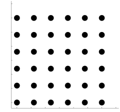
(a) $\lambda_{1}/\lambda_{2}=0$

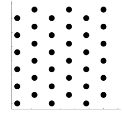
(b) $\lambda_{1}/\lambda_{2}=1/2$

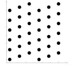
(c) $\lambda_{1}/\lambda_{2}=1/3$

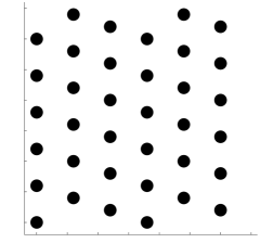
(d) $\lambda_{1}/\lambda_{2}=2/3$

Figure 1: The figure shows the placement of the Gabor atoms for four different lattice types in the time-frequency plane . The displayed Gabor system has parameters $a=6$, $M=6$ and $L=36$. The lattice (a) is called rectangular or separable and the lattice (b) is known as the quincunx lattice.

2.2 Metaplectics

A metaplectic operator, loosely speaking, is the signal domain counterpart to a symplectic transform of the lattice on phase space. A comprehensive treatment of these operators in the finite discrete setting can be found in [26]. In this contribution we will be focusing on the one dimensional setting, for which the operators are described in detail in [15]. In this section we will formulate some results that will prove to be important in subsequent sections. We start by the factorization of a lattice generator into elementary matrices, which we will denote by

$$\begin{split}\@ADDCLASS{ltx_eqn_lefteqn}$\displaystyle F=\left(\begin{array}[]{cc}0&-1\\ 1&0\end{array}\right),\quad S_{c}=\left(\begin{array}[]{cc}1&0\\ c&1\end{array}\right),$\mbox{}\hfil\hskip 40.0pt&\\ &D_{a}=\left(\begin{array}[]{cc}a&0\\ 0&a^{-1}\end{array}\right),\hskip 40.0pt\end{split}$$ (5)

where $c\in\mathbb{Z}_{L}$ and $a\in\mathbb{Z}_{L}$ invertible.

Proposition 3 (Feichtinger et al. (2008) [15]).

Let $M=\left(\begin{smallmatrix}a&b\\ c&d\end{smallmatrix}\right)\in\mathbb{Z}_{L}^{2}$ with $\det(M)=1$, then there exists $m\in\mathbb{Z}$ such that $a_{0}=a+mb$ is invertible in $\mathbb{Z}_{L}$. Let $c_{0}=c+md$, then

$$M=S_{c_{0}a_{0}^{-1}}D_{a_{0}}F^{-1}S_{-a_{0}^{-1}b}FS_{-m}.$$

The proof is based on Weil’s decomposition of arbitrary symplectic matrices into a composition of elementary symplectic matrices as in (5).

Lemma 1.

For the above defined matrices we define the corresponding metaplectic operators as follows

$$F \mapsto\mathbf{U}_{F}=\mathcal{F}$$

$$S_{c} \mapsto\mathbf{U}_{S_{c}}=\left(f(\cdot)\mapsto f(\cdot)\exp(\pi ic\cdot^{2}(L+1)/L)\right)$$

$$D_{a} \mapsto\mathbf{U}_{D_{a}}=\left(f(\cdot)\mapsto f(a^{-1}\cdot)\right).$$

With these transformations the following hold for all $\lambda\in\mathbb{Z}_{L}^{2}$

$$\mathbf{U}_{F}\pi(\lambda) =\phi_{F}(\lambda)\pi(F\lambda)\mathbf{U}_{F}$$

$$\mathbf{U}_{S_{c}}\pi(\lambda) =\phi_{S_{c}}(\lambda)\pi(S_{c}\lambda)\mathbf{U}_{S_{c}}$$

$$\mathbf{U}_{D_{a}}\pi(\lambda) =\phi_{D_{a}}(\lambda)\pi(D_{a}\lambda)\mathbf{U}_{D_{a}},$$

where $\phi_{F}$, $\phi_{S_{c}}$ and $\phi_{D_{a}}$ are phase factors.

Proof.

Some simple calculations are sufficient to establish the result:

$$\mathbf{U}_{F}\pi(\lambda)f =\mathcal{F}\mathbf{M}_{\omega}\mathbf{T}_{x}f=T_{\omega}M_{-x}\hat{f}$$

$$=e^{-2\pi ix\omega/L}\mathbf{M}_{-x}\mathbf{T}_{\omega}\hat{f}=e^{-2\pi ix\omega/L}\pi(F\lambda)\mathbf{U}_{F}f,$$

$$\mathbf{U}_{S_{c}}\pi(\lambda)f =\mathbf{M}_{\omega}\mathbf{T}_{x}e^{\pi ic(\cdot+x)^{2}(L+1)/L}f$$

$$=e^{\pi icx^{2}(L+1)/L}\mathbf{M}_{\omega+cx}\mathbf{T}_{x}\mathbf{U}_{S_{c}}f$$

$$=e^{\pi icx^{2}(L+1)/L}\pi(S_{c}\lambda)\mathbf{U}_{S_{c}}f$$

and

$$\mathbf{U}_{D_{a}}\pi(\lambda)f =\mathbf{M}_{a^{-1}\omega}f(a\cdot-x)=\mathbf{M}_{a^{-1}\omega}f\left(a^{-1}(\cdot-ax)\right)$$

$$=\mathbf{M}_{a^{-1}\omega}\mathbf{T}_{ax}\mathbf{U}_{D_{a}}f=\pi(D_{a}\lambda)\mathbf{U}_{D_{a}}f.$$

∎

The combination of the two results above immediately yields the following theorem.

Theorem 1.

For any matrix $M\in\mathbb{Z}_{L}^{2}$ with $\det(M)=1$, there exists a metaplectic operator $\mathbf{U}_{M}$, such that for all $\lambda\in\mathbb{Z}_{L}^{2}$

$$\mathbf{U}_{M}\pi(\lambda)=\phi_{M}(\lambda)\pi(M\lambda)\mathbf{U}_{M}.$$

3 Computation on nonseparable lattices

Nonseparable lattices in $\mathbb{Z}_{L}^{2}$ can be interpreted in a variety of ways. Several different approaches relate Gabor expansions on general lattices to one or several equivalent expansions on separable (or rectangular) lattices. From an algorithmic viewpoint, these are of particular interest, since a wealth of research [28, 2, 3, 41, 4, 34] has investigated efficient algorithms for analysis and synthesis using Gabor dictionaries on separable lattices. Each of the three approaches described in this section yields a simple relation between arbitrary given Gabor systems and Gabor systems on separable sampling sets that can be harnessed for efficient analysis and synthesis.

3.1 Correspondence via multiwindow Gabor

We will decompose a given lattice into a union of co-sets of a sparser separable lattice, which will allow us to use multiwindow methods [42, 43, 44, 45] for the computation. Using multiwindow methods for computation of Gabor transforms on nonseparable lattices has been proposed in [18, 43] and implementation has been discussed in [38, 36]. However, the latter only briefly mention the computation of dual Gabor windows, not discussing efficient implementation in detail.

Proposition 4.

Given the lattice $\Lambda$ in normal form specified by the parameters $a,b$ and $s$, then

$$\Lambda=\cup_{m=0}^{\lambda_{2}-1}\left((am,sm~{}\operatorname{mod}~{}b)^{T}+\tilde{\Lambda}\right),$$

where $\lambda_{2}=b/\gcd(b,s)$ and $\tilde{\Lambda}$ is the separable lattice generated by $(\lambda_{2}a,0)^{T}$ and $(0,b)$.

Proof.

Let the matrix generating $\Lambda$ be denoted by $A$ and let us define $M_{x}=\left\{sx+b\omega:\;\omega\in\mathbb{Z}_{L}\right\}$, for $0\leq x<L/a$. We note here, that $M_{x}$ is the second coordinate of the set $A\cdot(x,\mathbb{Z}_{L})^{T}$. Furthermore, $0\in M_{x}$ if and only if $x$ is a multiple of $\lambda_{2}$. To see that, we first note that $\lambda_{1}$ and $\lambda_{2}$ are relatively prime. Then the following equation has a solution if and only if $x$ is a multiple of $\lambda_{2}$

$$sx+b\omega=b\left(\frac{\lambda_{1}}{\lambda_{2}}x+\omega\right)=0.$$

This yields

$$M_{x} =M_{x+\lambda_{2}},\quad\text{for $x\in\mathbb{Z}_{L/a}$}$$

$$M_{x} =sx~{}\operatorname{mod}~{}b+M_{0}$$

This observation yields the following decomposition of the original lattice

$$\begin{split}\Lambda&=\bigcup_{x=0}^{L/a-1}\{ax\}\times M_{x}\\ &=\bigcup_{m=0}^{\lambda_{2}-1}\bigg{(}(am,sm~{}\operatorname{mod}~{}b)^{T}\\ &\hskip 40.0pt+\bigcup_{j=0}^{L/(a\lambda_{2})-1}\{aj\lambda_{2}\}\times M_{0}\bigg{)},\end{split}$$

which finishes the proof by observing

$$\tilde{\Lambda}=\bigcup_{j=0}^{L/(a\lambda_{2})-1}\{aj\lambda_{2}\}\times M_{0}.$$

∎

We can now describe a Gabor system $\mathcal{G}(g,\Lambda)$, with $\Lambda$ in the form (3), and the related operators completely in terms of a union of Gabor systems $\mathcal{G}(g_{m},\tilde{\Lambda})$ on the separable lattice $\tilde{\Lambda}$.

Proposition 5.

Let $\mathcal{G}(g,\Lambda)$, $\mathcal{G}(g_{m},\tilde{\Lambda})$, with $\Lambda,\tilde{\Lambda}$ as in Proposition 4 and $g\in\mathbb{C}^{L}$, $g_{m}=\mathbf{M}_{ms~{}\operatorname{mod}~{}b}\mathbf{T}_{ma}g$, for $0\leq m<\lambda_{2}$, be Gabor systems, then

$$\mathbf{S}_{g,\Lambda}f=\sum_{m=0}^{\lambda_{2}-1}\mathbf{S}_{g_{m},\tilde{\Lambda}}f.$$ (6)

Moreover, the Gabor transform can be computed using the identity

$$\begin{split}\@ADDCLASS{ltx_eqn_lefteqn}$\displaystyle\langle f,\mathbf{M}_{kb+(ms~{}\operatorname{mod}~{}b)}\mathbf{T}_{na}g\rangle$\mbox{}\hfil\\ &=e^{-2\pi i\tilde{n}\tilde{a}(ms~{}\operatorname{mod}~{}b)/L}\langle f,\mathbf{M}_{kb}\mathbf{T}_{\tilde{n}\tilde{a}}g_{m}\rangle,\end{split}$$ (7)

where $\tilde{n}=\lfloor n/\lambda_{2}\rfloor$ and $m=n-\tilde{n}$.

Proof.

Analogous to Lemma 1, we find that

$$\mathbf{M}_{kb+(ms~{}\operatorname{mod}~{}b)}\mathbf{T}_{na}g$$

$$=\mathbf{M}_{kb}\mathbf{M}_{ms~{}\operatorname{mod}~{}b}\mathbf{T}_{\tilde{n}\tilde{a}}\mathbf{T}_{ma}g$$

$$=e^{2\pi i\tilde{n}\tilde{a}(ms~{}\operatorname{mod}~{}b)/L}\mathbf{M}_{kb}\mathbf{T}_{\tilde{n}\tilde{a}}\mathbf{M}_{ms~{}\operatorname{mod}~{}b}\mathbf{T}_{ma}g$$

$$=e^{2\pi i\tilde{n}\tilde{a}(ms~{}\operatorname{mod}~{}b)/L}\mathbf{M}_{kb}\mathbf{T}_{\tilde{n}\tilde{a}}g_{m},$$

yielding (7). Using $kb+(ms~{}\operatorname{mod}~{}b)=kb+(ns~{}\operatorname{mod}~{}b)=(k-\lfloor ns/b\rfloor)b+ns$, since $\tilde{n}s~{}\operatorname{mod}~{}b=0$ allows to derive (6) by the identity

$$\begin{split}\@ADDCLASS{ltx_eqn_lefteqn}$\displaystyle\sum_{n=0}^{L/a-1}\sum_{k=0}^{L/b-1}\langle f,\mathbf{M}_{ns+kb}\mathbf{T}_{na}g\rangle\mathbf{M}_{ns+kb}\mathbf{T}_{na}g$\mbox{}\hfil\\ &=\sum_{m=0}^{\lambda_{2}-1}\sum_{\tilde{n}=0}^{L/\tilde{a}-1}\sum_{k=0}^{L/b-1}\langle f,\mathbf{M}_{kb}\mathbf{T}_{\tilde{n}\tilde{a}}g_{m}\rangle\mathbf{M}_{kb}\mathbf{T}_{\tilde{n}\tilde{a}}g_{m}.\end{split}$$

∎

3.2 Correspondence via Smith normal form

In this and the following section, we aim to describe an arbitrary lattice as separable lattice under a symplectic deformation, i.e. we will determine a symplectic matrix $P$, such that $\Lambda=P\tilde{\Lambda}$ for a general lattice $\Lambda$ and a separable lattice $\tilde{\Lambda}$. This problem is equivalent to decomposing the lattice generator matrix $A\in\mathbb{Z}_{L}^{2\times 2}$ into $A=PDV$, with a diagonal matrix $D$, a determinant $1$ matrix $V$ and a symplectic matrix $P$. We observed earlier that any determinant $1$ matrix in $\mathbb{Z}_{L}^{2\times 2}$ is symplectic. Thus, this decomposition is accomplished by applying Smith’s algorithm for matrices in $\mathbb{Z}^{2\times 2}$ to determine the Smith normal form $\tilde{D}$ of $A$ and transformation matrices $\tilde{P},\tilde{V}$, followed by considering the entries of $\tilde{D},\tilde{P},\tilde{V}$ modulo $L$ to find $D,P,V$.

The following Proposition by Feichtinger et al. was originally published in [15], where the proof is also presented. The procedure of computing Gabor transforms and dual windows using the methods in this section have been proposed therein, but their implementation was not discussed in detail.

Proposition 6.

Let $\Lambda=A\mathbb{Z}_{L}^{2}$ be a lattice and $A=\tilde{P}\tilde{D}\tilde{V}$ the Smith decomposition of $A$. Then

$$\Lambda=P\tilde{\Lambda},$$

where $P=(\tilde{P}~{}\operatorname{mod}~{}L)$, $D=(\tilde{D}~{}\operatorname{mod}~{}L)$ and $\tilde{\Lambda}=D\mathbb{Z}_{L}^{2}$.

Using Proposition 3 and Lemma 1 one obtains the operator $\mathbf{U}_{P}$ corresponding to the symplectic matrix $P$ and this leads to the final computational procedure described in the following Corollary.

Corollary 1.

Let the notation be as in the previous proposition. Then one finds for the symplectic matrix $P$ and the corresponding metaplectic operator $\mathbf{U}_{P}$ by setting $\tilde{g}=\mathbf{U}_{P}^{-1}g$

$$\mathbf{S}_{g,\Lambda}=\mathbf{U}_{P}\mathbf{S}_{\tilde{g},\tilde{\Lambda}}\mathbf{U}_{P}^{-1}.$$

Furthermore, the Gabor coefficients can be computed using the identity

$$\langle f,\pi\left(z\right)g\rangle=\phi_{P}(z)\langle\mathbf{U}_{P}^{-1}f,\pi\left(P^{-1}z\right)\tilde{g}\rangle,$$

for all $z=(x,\omega)^{T}\in\Lambda$.

3.3 Correspondence via shearing

As detailed in the previous section, the Weil decomposition and Smith normal form can be used to show that any lattice in $\mathbb{Z}^{2}_{L}$ can be written as a separable lattice, deformed by $6$ elementary symplectic matrices. This number can be reduced to $4$ or less as shown in the following theorem, which we will prove at the end of this section. Reducing computations on nonseparable lattices to the product lattice case via a shear operation has been proposed earlier [38, 36], however the authors were able to describe only a subset of all lattices over $\mathbb{Z}^{2}_{L}$ as shears of rectangular lattices. In [36] the author speculates that it might be possible to describe every lattice a the image of a product lattice under a horizontal and a vertical shear. In this section, we prove that this is indeed possible.

The proper definition of discrete, finite chirps, necessary to perform time-frequency shearing, has been a matter of some discussion, see e.g. [9]. While the naive linear chirp $\exp(2\pi ist^{2}/L)$ is still used by Bastiaans and van Leest [38, 36], a more appropriate definition, see Lemma 1, has been proposed by Kaiblinger [25, 15], constituting a second degree character [39].

Theorem 2.

let $A\in\mathbb{Z}_{L}^{2\times 2}$. There exist $s_{0},s_{1}\in\mathbb{Z}_{L}$ and $V\in\mathbb{Z}_{L}^{2\times 2}$ with $|\det(V)|=1$, such that

$$A=U_{s_{0},s_{1}}DV,$$ (8)

where $D\in\mathbb{Z}_{L}^{2\times 2}$ is diagonal and

$$U_{s_{0},s_{1}}=S_{-s_{1}}F^{-1}S_{s_{0}}F$$ (9)

We can now rewrite Gabor transforms on nonseparable lattices in the vein of Proposition 1 using the metaplectic operator associated to $U_{s_{0},s_{1}}$. Subsequently, we denote by $\mathbf{U}_{s_{0},s_{1}}$ the metaplectic operator associated with $U_{s_{0},s_{1}}$.

Proposition 7.

Let $\Lambda=A\mathbb{Z}_{L}^{2}$ be a lattice, $D,U_{s_{0},s_{1}}$ as in the previous theorem and $\tilde{\Lambda}=D\mathbb{Z}_{L}^{2}$. Furthermore let $g\in\mathbb{C}^{L}$ and $\tilde{g}=\mathbf{U}_{{s_{0},s_{1}}}^{-1}g$. Then

$$\mathbf{S}_{g,\Lambda}f =\mathbf{U}_{{s_{0},s_{1}}}\mathbf{S}_{\tilde{g},\tilde{\Lambda}}\mathbf{U}_{{s_{0},s_{1}}}^{-1}f$$ (10)

and

$$\begin{split}\@ADDCLASS{ltx_eqn_lefteqn}$\displaystyle\langle f,\mathbf{M}_{\omega}\mathbf{T}_{x}g\rangle$\mbox{}\hfil\\ &=\phi_{U_{s_{0},s_{1}}}(z)\langle\mathbf{U}_{{s_{0},s_{1}}}^{-1}f,\mathbf{M}_{\omega-s1(x-s_{0}\omega)}\mathbf{T}_{x-s_{0}\omega}\tilde{g}\rangle,\end{split}$$ (11)

for all $z=(x,\omega)^{T}$. Moreover,

$$\phi_{U_{s_{0},s_{1}}}(z)=e^{\pi i(s_{0}\omega^{2}-s_{1}(x-s_{0}\omega)^{2})(L+1)/L}.$$ (12)

Proof.

Everything but the explicit form of the phase factor $\phi_{U_{s_{0},s_{1}}}$ is a direct consequence of Lemma 1 and Theorem 2, note

$$U_{s_{0},s_{1}}=S_{-s_{1}}F^{-1}S_{s_{0}}F=\begin{pmatrix}1&-s_{0}\\ -s_{1}&s_{0}s_{1}+1\end{pmatrix}.$$

To complete the proof, set $y=(x-s_{0}\omega)$ and determine the phase factor explicitly:

$$\mathbf{U}_{S_{-s_{1}}}\mathcal{F}^{-1}\mathbf{U}_{S_{s_{0}}}\mathcal{F}\mathbf{M}_{\omega}\mathbf{T}_{x}f$$

$$=e^{\pi is_{0}\omega^{2}(L+1)/L}\mathbf{U}_{S_{-s_{1}}}\mathcal{F}^{-1}\mathbf{T}_{\omega}\mathbf{M}_{s_{0}\omega-x}\mathbf{U}_{S_{s_{0}}}\mathcal{F}f$$

$$=e^{\pi is_{0}\omega^{2}(L+1)/L}\mathbf{U}_{S_{-s_{1}}}\mathbf{M}_{\omega}\mathbf{T}_{y}\mathcal{F}^{-1}\mathbf{U}_{S_{s_{0}}}\mathcal{F}f$$

$$=e^{\pi i(s_{0}\omega^{2}-s_{1}y^{2})(L+1)/L}\mathbf{M}_{\omega-s_{1}y}\mathbf{T}_{y}\mathbf{U}_{S_{-s_{1}}}\mathcal{F}^{-1}\mathbf{U}_{S_{s_{0}}}\mathcal{F}f,$$

where we used Lemma 1 and $\exp(2\pi im(L+1)/L)=\exp(2\pi im/L)$ for all $m\in\mathbb{Z}$. ∎

For Proposition 7 to be valid, it remains to prove Theorem 2, establishing the representation of $A$ through $U_{s_{0},s_{1}}$.

Proof of Theorem 2.

By Proposition 1 we can assume without loss of generality that $A$ is in lattice normal form, i.e.

$$A=\begin{pmatrix}a&0\\ s&b\end{pmatrix}.$$

To prove equation (8), we rewrite $U^{-1}_{s_{0},s_{1}}A=DV$ with a diagonal matrix $D$ and a unitary matrix $V$. It can be seen that

$$U^{-1}_{s_{0},s_{1}}=\left(\begin{array}[]{cc}s_{0}s_{1}+1&s_{0}\\ s_{1}&1\end{array}\right)=\left(\begin{array}[]{cc}1&s_{0}\\ 0&1\end{array}\right)\left(\begin{array}[]{cc}1&0\\ s_{1}&1\end{array}\right).$$

Now, using Proposition 2 in the step from 24 to 31 below, we can write

$$U^{-1}_{s_{0},s_{1}}A =\hbox to0.0pt{$\displaystyle\left(\begin{array}[]{cc}1&s_{0}\\ 0&1\end{array}\right)\left(\begin{array}[]{cc}1&0\\ s_{1}&1\end{array}\right)\left(\begin{array}[]{cc}a&0\\ s&b\end{array}\right)$\hss}$$ (19)

$$=\left(\begin{array}[]{cc}1&s_{0}\\ 0&1\end{array}\right)\left(\begin{array}[]{cc}a&0\\ s_{1}a+s&b\end{array}\right)$$ (24)

$$=\left(\begin{array}[]{cc}1&s_{0}\\ 0&1\end{array}\right)\left(\begin{array}[]{cc}\frac{ab}{X}&ak_{1}\\ 0&X\end{array}\right)\left(\begin{array}[]{cc}k_{2}&-k_{1}\\ Y&b/X\end{array}\right)$$ (31)

$$=\left(\begin{array}[]{cc}\frac{ab}{X}&s_{0}X+ak_{1}\\ 0&X\end{array}\right)\left(\begin{array}[]{cc}k_{2}&-k_{1}\\ Y&b/X\end{array}\right).$$ (36)

Here $X=\gcd(s_{1}a+s,b)$, $Y=X^{-1}(s_{1}a+s)$ and $k_{1},k_{2}$ stem from Bézout’s identity when representing $\gcd(s_{1}a+s,b)=k_{1}(s_{1}a+s)+k_{2}b$. It is important to note that the second matrix in the last line has determinant one. This shows that the lattice $U_{s_{0},s_{1}}A$ is separable if and only if $\tilde{D}=\left(\begin{smallmatrix}ab/X&s_{0}X+ak_{1}\\ 0&X\end{smallmatrix}\right)$ is equivalent to a diagonal matrix, i.e.

$$~{}\operatorname{mod}~{}(s_{0}X+ak_{1},ab/X)=0.$$ (37)

We will now deduce numbers $s_{0}$ and $s_{1}$ satisfying the our needs from the prime factor decomposition of the involved quantities. Therefore we represent $L=\prod_{j=1}^{J}p_{j}^{n_{j}}$ for a fixed set of prime numbers. Since $a$ and $b$ are divisors of $L$ we find their prime factor decompositions to have exponents $\{\alpha_{j}\}_{j=1}^{J}$ and $\{\beta_{j}\}_{j=1}^{J}$, where $\alpha_{j},\beta_{j}\leq n_{j}$. The shearing parameter has the decomposition $s=l\prod_{j=1}^{J}p_{j}^{\sigma_{j}}$, where $\gcd(l,L)=1$.

We choose

$$s_{1}=\prod_{j=1}^{J}p_{j}^{\mu_{j}}\text{, where }\mu_{j}=\begin{cases}1\text{ for }\alpha_{j}=\sigma_{j}\\ 0\text{ else.}\end{cases}$$ (38)

With this choice of $s_{1}$ we investigate

$$X=\gcd(s_{1}a+s,b)=\prod_{j=1}^{J}\gcd(s_{1}a+s,p_{j}^{\beta_{j}}).$$

To do so, we have to individually treat three cases:

1. $\alpha_{j}<\sigma_{j}$: Since $s_{1}$ and $p_{j}$ are coprime we find $\gcd(s_{1}a+s,p_{j}^{\beta_{j}})=p_{j}^{\min(\alpha_{j},\beta_{j})}$.

2. $\alpha_{j}>\sigma_{j}$: $\gcd(s_{1}a+s,p_{j}^{\beta_{j}})=p_{j}^{\min(\sigma_{j},\beta_{j})}$, and $\min(\sigma_{j},\beta_{j})<\alpha_{j}$

3. $\alpha_{j}=\sigma_{j}$: Use Eq. (38) to determine that $\gcd(s_{1}a+s,p_{j}^{\beta_{j}})=p_{j}^{\min(\alpha_{j},\beta_{j})}$

The above arguments show that with the choice of $s_{1}$, we find that $X=\prod_{j=1}^{J}p_{j}^{\gamma_{j}}$, where $\gamma_{j}\leq\alpha_{j}$.

Now we turn to the choice of $s_{0}$. To do so we first decompose $k_{1}=l\prod_{j=1}^{J}p_{j}^{\kappa_{j}}$, where $l$ and $L$ are coprime. Let us explain how to choose the shear via the positive part of a vector

$$s_{0}=\left(\prod_{j=1}^{J}p_{j}^{(\beta_{j}-\gamma_{j}-\kappa_{j})_{+}}-l\right)\prod_{j=1}^{J}p_{j}^{\alpha_{j}+\kappa_{j}-\gamma_{j}},$$

where $(x_{+})_{j}=\max(x_{j},0)$. A straightforward calculation shows then that

$$s_{0}X+ak_{1}=\prod_{j=1}^{J}p_{j}^{(\beta_{j}-\gamma_{j}-\kappa_{j})_{+}+\alpha_{j}+\kappa_{j}},$$

and we furthermore see that

$$(\beta_{j}-\gamma_{j}-\kappa_{j})_{+}+\alpha_{j}+\kappa_{j}\geq\beta_{j}+\alpha_{j}-\gamma_{j}.$$

This proofs that (37) is satisfied, completing the proof. ∎

Remark 1.

It is easy to see that $X$ in the proof above satisfies $\gcd(a,b)=kX$ for some $k\in\mathbb{N}_{0}$ and therefore $ab/X$ is a multiple of $X$. Thus, the diagonal matrix constructed above is in fact the Smith normal form of $A$.

3.4 Further optimization

In this section we will first determine which signal lengths are feasible for some given choice of $a,M$ and $\lambda_{1},\lambda_{2}$. This restriction holds for all the presented methods equally and is essential to know in computations.

Particularly when using the shear method described in Subsection 3.3 it is interesting to know for which signal lengths one of the two shears $s_{0}$ and $s_{1}$, preferably the frequency side shear $s_{0}$, can be chosen to be zero. This saves additional computation time.

Proposition 8.

Given the parameters $\lambda=\lambda_{1}/\lambda_{2}$, $a$ and $M$. Then the minimal signal length, for which these parameters are feasible is given by $L_{\text{min}}=\lambda_{2}\operatorname{lcm}\left(a,M\right)$. All the feasible signal lengths are multiples of this.

Proof.

For the parameters in combination with a given signal length $L$ to form a lattice we require the following conditions

$$\begin{split}a|L,\;M|L\\ \frac{L}{a}\lambda\in\mathbb{Z}\\ \frac{L}{M}\lambda\in\mathbb{Z},\end{split}$$

where the first conditions immediately yield $\operatorname{lcm}\left(a,M\right)|L$. From the other two conditions we can derive

$$a\lambda_{2}/\gcd(a,\lambda_{1})|L\quad\text{ and }\quad M\lambda_{2}/\gcd(M,\lambda_{1})|L.$$

Therefore, the signal length has to be a multiple of

$$L_{\text{min}}=\operatorname{lcm}\left(\frac{a\lambda_{2}}{\gcd(a,\lambda_{1})},\frac{M\lambda_{2}}{\gcd(M,\lambda_{1})},a,M\right).$$

We proceed to show that

$$\operatorname{lcm}\left(\frac{a\lambda_{2}}{\gcd(a,\lambda_{1})},a\right)=\lambda_{2}a.$$ (39)

For this purpose we look at the prime factor decomposition of the involved quantities, where we denote by $\alpha_{j},\gamma_{j},\delta_{j}$ the exponents of the prime number $p_{j}$ of $a,\lambda_{1}$ and $\lambda_{2}$ respectively. Then we find, since $\lambda_{1}$ and $\lambda_{2}$ are co-prime that the exponent of $p_{j}$ of $\operatorname{lcm}\left(a\lambda_{2}/\gcd(a,\lambda_{1}),a\right)$ is given by

$$\max(\alpha_{j}-\min(\alpha_{j},\gamma_{j})+\delta_{j},\alpha_{j})=\alpha_{j}+\delta_{j},$$

proving (39). The proof that $\operatorname{lcm}\left(M\lambda_{2}/\gcd(M,\lambda_{1}),M\right)=\lambda_{2}M$ is completely analogous. Combine these to find

$$\begin{split}\@ADDCLASS{ltx_eqn_lefteqn}$\displaystyle\operatorname{lcm}\left(\frac{a\lambda_{2}}{\gcd(a,\lambda_{1})},\frac{M\lambda_{2}}{\gcd(M,\lambda_{1})},a,M\right)$\mbox{}\hfil\\ &=\operatorname{lcm}\left(\lambda_{2}a,\lambda_{2}M\right)=\lambda_{2}\operatorname{lcm}\left(a,M\right).\end{split}$$

∎

Now we shall investigate, which multiples of the just derived minimal signal length allow for computation without the frequency shear. To do so, it is instructive to compute the set of factors $l$, for which $L=lL_{\text{min}}$ needs only the time shear. We will introduce here some important constants related to the time shift $a$, the frequency shift $b$, the number of channels $M=L/b$ and the number of time shifts $N=L/a$. We define $c,d,p,q\in\mathbb{N}$ by

$$c=\gcd\left(a,M\right) d=\gcd\left(b,N\right),$$ , (40)

$$p=\frac{a}{c}=\frac{b}{d} q=\frac{M}{c}=\frac{N}{d}.$$ , (41)

With these numbers, the redundancy of a Gabor system can be written as $L/\left(ab\right)=q/p,$ where $q/p$ is an irreducible fraction. It holds that $L=cdpq$. Some of the introduced notation will be important in the next section.

Proposition 9.

Given $\lambda$, $a$ and $M$. Let the prime factor decomposition of $c=\gcd(a,M)$ be given by

$$c=\prod_{j=1}^{J}p_{j}^{\gamma_{j}}$$

for some set of prime factors and corresponding exponents. Let

$$c_{1}=\prod_{j=1}^{J}p_{j}^{\sigma_{j}},\quad\sigma_{j}=\begin{cases}\gamma_{j}\quad&\text{if $\gcd(\lambda_{2},p_{j})=0$}\\ 0&\text{else},\end{cases}$$

then the frequency shear can be chosen to be $0$ if the signal length satisfies

$$L=nL_{\text{min}}\frac{c}{c_{1}},$$ (42)

for some $n\in\mathbb{N}$. In words, $c_{1}$ are factors of $c$ that are relatively prime to $\lambda_{2}$

Proof.

With the standard notation we easily see that the time shear is sufficient if and only if $(s+kb)/a\in\mathbb{Z}$ for some $k\in\{0,\ldots,M-1\}$. Rewriting this leads to

$$L=\tilde{l}\frac{Ma\lambda_{2}}{\lambda_{1}+k\lambda_{2}}=l\frac{Ma\lambda_{2}}{\gcd(\lambda_{1}+k\lambda_{2},Ma\lambda_{2})},$$

for some $l\in\mathbb{Z}$. However, these signal lengths might not be compatible with the feasibility condition from Proposition 8. Therefore we compute the ratio

$$\frac{L}{L_{\text{min}}}=l\frac{\gcd(M,a)}{\gcd(\lambda_{1}+k\lambda_{2},Ma\lambda_{2})}.$$

Since this fraction should be an integer number, we have to choose

$$l=n\frac{\gcd(\lambda_{1}+k\lambda_{2},Ma\lambda_{2})}{\gcd(M,a,\lambda_{1}+k\lambda_{2},Ma\lambda_{2})},$$

for some $n\in\mathbb{N}$. Therefore, we can compute

$$L=nL_{\text{min}}\frac{\gcd(M,a)}{\gcd(M,a,\lambda_{1}+k\lambda_{2})}.$$ (43)

With the notation introduced above we are now interested in computing

$$\max_{k\in\mathbb{N}}(\gcd(c,\lambda_{1}+k\lambda_{2})).$$ (44)

Firstly, we rewrite

$$\gcd(c,\lambda_{1}+k\lambda_{2})=\prod_{j=1}^{J}\gcd(p_{j}^{\gamma_{j}},\lambda_{1}+k\lambda_{2}).$$

Now we will individually investigate the factors in the product above.

Case 1. $\gcd(p_{j},\lambda_{2})=1$, in which case we can find numbers $k_{1,j},k_{2,j}$, such that

$$\lambda_{1}+k_{1,j}\lambda_{2}=k_{2,j}p_{j}^{\gamma_{j}}.$$

Furthermore, the full set of coefficients of $\lambda_{2}$, for which the above equation can be satisfied is given by $K_{j}=\left\{k_{1,j}+mp_{j}^{\gamma_{j}}:m\in\mathbb{Z}\right\}$. Therefore, for any $k\in K_{j}$ we find

$$\gcd(p_{j}^{\gamma_{j}},\lambda_{1}+k\lambda_{2})=p_{j}^{\gamma_{j}}.$$

Case 2. $\gcd(p_{j},\lambda_{2})\neq 1$, which implies directly that $\lambda_{2}$ is a multiple of $p_{j}$. In this case we have to argue that $\lambda_{1}+k\lambda_{2}$ can never be multiple of $p_{j}$. Indeed, any linear combination $k_{1,j}\lambda_{2}+k_{2,j}p_{j}$ is a multiple of $p_{j}$ and therefore not equal to $\lambda_{1}$, which is assumed to be relatively prime to $\lambda_{2}$. Consequently, for any choice of $k\in\mathbb{Z}$

$$\gcd(p_{j}^{\gamma_{j}},\lambda_{1}+k\lambda_{2})=1.$$

For all the indices $j$ in case $1$, it is easy to see that the intersection of the corresponding sets $K_{j}$ is not empty. This is an immediate consequence from the fact that powers of two different prime numbers have no common divisors. Using the notation introduced above, we can conclude that there exists some $k\in\mathbb{Z}$, such that

$$\gcd(c,\lambda_{1}+\lambda_{2})=c_{1}.$$

The last argument needed is to show that $k\in\left\{0,\ldots,M-1\right\}$. By construction $s+kb=\tilde{k}a$, for some $\tilde{k}\in\mathbb{Z}$. Therefore, for any $m\in\mathbb{Z}$

$$s+\left(k+m\frac{L}{b}\right)b=\left(\tilde{k}+m\frac{L}{a}\right)a,$$

and for an appropriate choice of $m$, the expression in brackets on the left hand side will evaluate some number in the desired range.

∎

Remark 2.

There are possibly other feasible signal lengths than determined by (42). The full set of feasible lengths is determined by

$$\left\{nL_{\text{min}}\frac{\gcd(M,a)}{\gcd(M,a,\lambda_{1}+k\lambda_{2})}:\;n\in\mathbb{N},k\in\left\{0,\ldots,M-1\right\}\right\}.$$

This can be easily seen from (43) in the proof above. For simplicity we only construct the minimal factor, that $L_{\text{min}}$ has to be multiplied with, as stated in (44).

Remark 3.

Looking at (42) we see that if we are given a certain redundancy (41) $q/p$ and a lattice type $\lambda_{1}/\lambda_{2}$ and want to get a low value of $L_{min}c/d$ we must choose $c$ such that it is relatively prime to $\lambda_{2}$. As an example, consider a common choice of $a=32$, $M=64$ and $\lambda_{1}/\lambda_{2}=1/2$ (the quincunx lattice). In this case $c=\gcd(a,M)=32$ which is the worst possible case, as it is a power of $\lambda_{2}=2$ giving a value of $L_{min}c/d=128\cdot 32=4096$. If we instead choose $a=27$, $M=54$ (which is the same redundancy) we get $L_{min}c/d=108\cdot 1=108$. This illustrates that it is possible to work efficiently with the quincunx lattice by not choosing the rectangular lattice parameters to be powers of 2.

3.5 Extension to higher dimensions

It is well known [27, 10, 16] that multidimensional Gabor transforms and dual windows can be computed using algorithms designed for the $1$D case, if both the Gabor window and the lattice used can be written as a tensor product. That is, we assume that with $l=(l_{1},\ldots,l_{n})^{T}\in\mathbb{C}^{L_{1}}\times\ldots\times\mathbb{C}^{L_{n}}$,

$$g(l)=g_{1}(l_{1})\otimes\ldots\otimes g_{n}(l_{n})$$

and

$$\Lambda=\Lambda_{1}\times\ldots\times\Lambda_{n}=A_{1}\mathbb{Z}^{2}_{L_{1}}\times\ldots\times A_{n}\mathbb{Z}^{2}_{L_{n}}$$

for some $A_{j}\in\mathbb{Z}^{2}_{L_{j}}\times\mathbb{Z}^{2}_{L_{j}}$ for $j=1,\ldots,n$.

Equivalently, we can say that $\Lambda$ can be described by a block matrix

$$A=\left(\begin{array}[]{cc}D&E\\ F&G\end{array}\right).$$ (45)

with diagonal blocks $D,E,F,G\in\mathbb{Z}^{n\times n}$. In this case, the multidimensional transform and dual window can be computed by subsequently applying the algorithms presented in the previous sections in every dimension. A matrix describing the lower dimensional lattice corresponding to dimension $j$ is simply given by

$$A_{j}=\left(\begin{array}[]{cc}D_{j,j}&E_{j,j}\\ F_{j,j}&G_{j,j}\end{array}\right)$$

and can be transformed into lattice normal form (3), allowing straightforward application of the presented algorithms.

However, we are not aware of a constructive method to determine whether a lattice, given by an arbitrary matrix, can be described by a banded matrix of the form (45).

In contrast to the methods based on metaplectic operators, it is easier to extend the multiwindow approach from 3.1 to higher dimensions. For reasons of readability we will not give details here.

4 Implementation and timing

In this section we discuss the implementation and speed of the proposed algorithms. It is important for this section to recall the definition of the constants $c,d$ in 40 and $p,q$ in (41).

Methodology for computing the computational complexity. To compute the Discrete Fourier transform, the familiar FFT algorithm is used. When computing the flop (floating point operations) count of the algorithm, we will assume that a complex FFT of length $M$ can be computed using $4M\log_{2}M$ flops. A review of flop counts for FFT algorithms is presented in [24]. When computing the flop count, we assume that both the window and signal are complex valued.

The cost of performing the computation of a DGT with a full length window on a rectangular lattice using the algorithm first reported in [32] is given by

$$8Lq+4L\log_{2}d+4MN\log_{2}d+4MN\log_{2}\left(M\right)$$ (46)

$$=L\left(8q+4\log_{2}d\right)+4MN\left(\log_{2}L/p\right)\hskip 40.0pt$$ (47)

where the first terms in (46) come from the multiplication of the matrices in the factorization, the two middle terms come from creating the factorization of the signal and inverting the factorization of the coefficients, and the last term comes from the final application of FFTs. The terms can be collected as in (47), where the first term grows as the length of the signal $L$, and the second terms grows as the total number of coefficients $MN$. In the following, we refer to this as the full window algorithm.

If the window is an FIR window supported on an index set with width $L_{g}$ which is much smaller than the length of the signal $L$, the weighted-overlap-add algorithm, first reported in [28], can be used instead. It has a computational complexity of

$$8L\frac{L_{g}}{a}+4NM\log_{2}M.$$

In the following, we refer to this as the FIR window algorithm.

A third approach to computing a DGT is a hybrid approach, where a DGT using an FIR window can be computing using a full window algorithm on blocks of the input signal. The blocks are then combined using the classical overlap-add algorithm, cf. [33, 22].

The OLA algorithm works by partitioning a system of length $L$ into blocks of length $L_{b}$ such that $L=L_{b}N_{b}$, where $N_{b}$ is the number of blocks. The block length must be longer than the support of the window, $L_{b}>L_{g}$. To perform the computation we take a block of the input signal of length $L_{b}$ and zero-extend it to length $L_{x}=L_{b}+L_{g}$, and compute the convolution with the extended signal using the similarly extended window. Because of the zero-extension of the window and signal, the computed coefficients will not be affected by the periodic boundary conditions, and it is therefore possible to overlay and add the computed convolutions of length $L_{x}$ together to form the complete convolution of length $L$.

The equations (47), (4) are used to express the efficiency of the algorithms for the DGT on nonseparable lattices.

4.1 Implementation of the shear algorithm

The shear algorithm proposed in Proposition 7 computes the DGT on a nonseparable lattice using a DGT on a separable lattice with some suitable pre- and postprocessing steps. The computational complexity of the pre- and postprocessing steps is significant compared to the separable DGT, so we wish to minimize the cost of these steps. An implementation of the shear algorithm is presented as Algorithm 1. Note that we assume the existence of several underlying routines: An implementation dgt of the separable Gabor transform, the periodic chirp pchirp(L,s)$=\exp(\pi is\cdot^{2}(L+1)/L)$ and shearfind, a program that determines the shear parameters $s_{0},s_{1}$ and the correct separable lattice to do the DGT on, following the constructive proof of Theorem 2.

Algorithm 1 The shear algorithm: $c=\textsc{dgtns}(f,g,a,M,\lambda)$

1:$\left[s_{0},s_{1},b_{r}\right]=\textsc{shearfind}(L,a,M,\lambda)$

2:if $s_{1}\neq 0$ then

3:     $p\leftarrow\textsc{pchirp}(L,s_{1})$

4:     $g(\cdot)\leftarrow p(\cdot)g(\cdot)$

5:     $f(\cdot)\leftarrow p(\cdot)f(\cdot)$

6:end if

7:if $s_{0}=0$ then

8:     $c_{r}\leftarrow\textsc{dgt}(f,g,a,M)$

9:     $C_{1}\leftarrow s_{1}a(L+1)\pmod{2N}$

10:     for $k=0\to N-1$ do

11:         $E\leftarrow e^{\pi i(C_{1}k^{2}\pmod{2N})/N}$

12:         for $m=0\to M-1$ do

13:              $c(\left\lfloor\frac{-s_{1}ka+mb\pmod{L}}{b}\right\rfloor,k)\leftarrow Ec_{r}(m,k)$

14:         end for

15:     end for

16:else

17:     $a_{r}\leftarrow\frac{ab}{b_{r}},\quad M_{r}\leftarrow\frac{L}{b_{r}},\quad N_{r}\leftarrow\frac{L}{a_{r}}$

18:     $C_{1}\leftarrow\frac{a_{r}}{a},\quad C_{2}\leftarrow-s_{0}b_{r}/a$

19:     $C_{3}\leftarrow as_{1}(L+1),\quad C_{4}\leftarrow C_{2}b_{r}(L+1)$

20:     $C_{5}\leftarrow 2C_{1}b_{r},\quad C_{6}\leftarrow(s_{0}s_{1}+1)b_{r}$

21:     $p\leftarrow\textsc{pchirp}(L,-s_{0})$

22:     $g(\cdot)\leftarrow p(\cdot)\textsc{fft}(g(\cdot))/L$

23:     $f(\cdot)\leftarrow p(\cdot)\textsc{fft}(f(\cdot))$

24:     $c_{r}\leftarrow\textsc{dgt}(f,g,b_{r},N_{r})$

25:     for $k=0\to N_{r}-1$ do

26:         for $m=0\to M_{r}-1$ do

27:              $s_{q1}\leftarrow C_{1}k+C_{2}m\pmod{2N}$

28:              $E\leftarrow e^{\pi i(C_{3}s_{q1}^{2}-m(C_{4}m+C_{5}k)\pmod{2N})/N}$

29:              $\tilde{m}\leftarrow C_{1}k+C_{2}m\pmod{N}$

30:              $\tilde{k}\leftarrow\left\lfloor\frac{-s_{1}a_{r}k+C_{6}m\pmod{L}}{b}\right\rfloor$

31:              $c(\tilde{k},\tilde{m})\leftarrow Ec_{r}(-k\pmod{N_{r}},m)$

32:         end for

33:     end for

34:end if

A simple trick is to notice that when a frequency-side shear is needed, the DFT of the signal $f$ and the window $g$ are multiplied by a chirp on the frequency side, $\tilde{f}=\mathbf{U}_{s_{0},s_{1}}^{-1}f$ and $\tilde{g}=\mathbf{U}_{s_{0},s_{1}}^{-1}g$. The total cost of this is 4 FFT’s and two pointwise multiplications. However, instead of transforming the chirped signal and window back to the time domain, we can compute the nonseparable DGT directly in the frequency domain using the well-known commutation relation of the DFT and the translation and modulation operators:

$$\left\langle f,M_{m}T_{n}g\right\rangle = e^{-\pi imn/L}\left\langle\mathcal{F}f,M_{-n}T_{m}\mathcal{F}g\right\rangle$$ (48)

This trick saves the two inverse FFTs at the expense of the multiplication of the coefficients by a complex exponential and reshuffling. As we already need these operations to realize (11) and (12), they can be combined with no additional computational complexity.

The overlap-add algorithm can be used in conjunction with the shear algorithm in the following case: we wish to compute the DGT with an FIR window for a nonseparable lattice using the shear algorithm. Because of the frequency-side shearing, the window is converted from an FIR window into a full length window, making it impossible to perform real-time or block-wise processing. However, if the shear algorithm is used inside an OLA algorithm, this is no longer a concern, as the shearing will only convert the window into a window of length $L_{g}+L_{b}$, restoring the ability to perform block-wise processing.

In total, the shear-OLA algorithm for the DGT is calculated in three steps using the three algorithms:

1. Split the input signal into blocks using the overlap-add algorithm

2. Apply the shears to the blocks of the input signal as in the shear algorithm

3. Use the full-window rectangular lattice DGT on the sheared signal blocks.

The downside of the shear-OLA algorithm is that the total length of the DGTs is longer than the original DGT by

$$\rho=\frac{L_{g}+L_{b}}{L_{b}},$$ (49)

where $L_{b}$ is the block length. Therefore, a trade-off between the block length and the window length must be found, so that the block length is long enough for (49) to be close to one, but at the same time small enough to not impose a too long processing delay.

4.2 Dual and tight windows

The shear method in Proposition 7 can also be used to compute the canonical dual and canonical tight windows, using the factorization of the frame operator given in (10). The complete algorithm for the canonical dual window is shown in 2, and uses the same trick as the Gabor transform algorithm to compute the canonical dual when a frequency side shear is needed: do it in the Fourier domain without transforming back. Again, we assume the existence of an implementation gabdual for the computation of Gabor dual windows on separable lattices.

Algorithm 2 Dual window via shearing:
$\tilde{g}=\textsc{gabdualns}(g,a,M,\lambda)$

1:$\left[s_{0},s_{1},b_{r}\right]=\textsc{shearfind}(L,a,M,\lambda)$

2:if $s_{1}\neq 0$ then

3:     $p\leftarrow\textsc{pchirp}(L,s_{1})$

4:     $g(\cdot)\leftarrow p(\cdot)g(\cdot)$

5:end if

6:$b\leftarrow\frac{L}{M},\quad M_{r}\leftarrow\frac{L}{b_{r}},\quad a_{r}\leftarrow\frac{ab}{b_{r}}$

7:if $s_{0}=0$ then

8:     $g_{d}\leftarrow\textsc{gabdual}(g,a_{r},M_{r})$

9:else

10:     $p_{0}\leftarrow\textsc{pchirp}(L,-s_{0})$

11:     $g(\cdot)\leftarrow p_{0}(\cdot)\textsc{fft}(g)(\cdot)$

12:     $g_{d}\leftarrow L\cdot\textsc{gabdual}(g,L/M_{r},L/a_{r})$

13:     $g_{d}\leftarrow\textsc{ifft}(\overline{p_{0}}(\cdot)g_{d}(\cdot))$

14:end if

To compute the canonical dual and tight windows on a separable lattice, the matrices are first factorized as in [34, 32] and then the factorized matrices are transformed as in [23].

4.3 Analysis of the computational complexity

Table 1: Flop counts for different ways of computing the DGT on a nonseparable lattice. First column list the algorithm, second column the flop count for the particular algorithm. Listed from the top, the algorithms are: The multiwindow algorithm using the full window rectangular lattice algorithm, the multiwindow algorithm using the FIR window rectangular lattice algorithm, the Smith normal form algorithm using the full window rectangular lattice algorithm, the shear algorithm when no frequency shear is needed, the shear algorithm including the frequency shear and finally the overlap-add versions of the shear algorithms. The term $L_{g}$ denotes the length of the window used so $L_{g}/a$ is the overlapping factor of the window.

Alg.:	Flop count
Multi-window
FIR.	$8L\frac{L_{g}}{a}+4NM\log_{2}M$
Full.	$L\lambda_{2}\left(8q_{mw}+4\log_{2}d_{mw}\right)$
	$+MN\left(4\log_{2}L/p_{mw}+6\right)$
SNF	$L\left(8q+4\log_{2}d_{sm}+8\log_{2}L+18\right)$
	$+MN\left(4\log_{2}L/p+6\right)$
Shear alg.
No freq. shear	$L\left(8q+4\log_{2}d+6k_{time}\right)$
	$+MN\left(4\log_{2}L/p+6k_{time}\right)$
Freq. shear	$L\left(8q+4\log_{2}Lc_{sh}+6+6k_{time}\right)$
	$+MN\left(4\log_{2}L/p+6\right)$
Shear OLA
No freq. shear	$\rho L\left(8q+4\log_{2}\rho d_{shola}+6k_{time}\right)$
	$+\rho MN\left(4\log_{2}\rho L_{b}/p+6k_{time}\right)$
Freq. shear	$\rho L\left(8q+4\log_{2}\rho Lc_{shola}+6k_{time}+6\right)$
	$+\rho MN\left(4\log_{2}\rho L_{b}/p+6\right)$

The flop counts of the various algorithms used for computing the DGT on a nonseparable lattice is listed in Table 1.

Based on the computational complexity presented in the table, any of the algorithms may for some specific problem setup be the fastest, except for the Smith-normal form algorithm which is always slower than the shear algorithm:

• The multiwindow algorithm for FIR windows is the fastest for very short windows.

• The multiwindow-OLA algorithm is the fastest for simple lattices ($\lambda_{2}$ small) and medium length windows.

• The shear-OLA algorithm is the fastest for more complex lattices ($\lambda_{2}$ large) and medium length windows.

• The multiwindow algorithm is the fastest for simple lattices ($\lambda_{2}$ small) and very long windows.

• The shear algorithm is the fastest for more complex lattices ($\lambda_{2}$ large) and very long windows.

4.4 Numerical experiments

Implementations of the algorithms described in this paper can be found in the Large Time Frequency Analysis Toolbox (LTFAT), cf. [31],[1]. An appropriate algorithm will be automatically invoked when calling the dgt or dgtreal functions. The implementations are done in both the Matlab / Octave scripting language and in C. All tests were performed on an Intel i7 CPU operating at 3.6 GHz.

As the speed of the algorithms depends on a large number of parameters $a$, $M$, $L$, $L_{g}$, $c$, $d$, $s_{0}$, $s_{1}$ and similar parameters relating to the multiwindow and shear transforms, we cannot provide an exhaustive illustration of the running times. Instead we will present some figures that illustrates the crossover point of when the the shear algorithm becomes faster than the multiwindow algorithm as the lattice complexity $\lambda_{2}$ increases. The behavior of the algorithms as the window length $L_{g}$ increases is completely determined by the algorithms for the rectangular lattice, so we refer to [32] for illustrations.

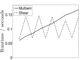
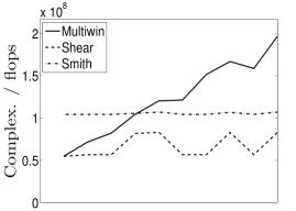
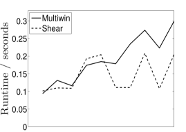
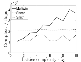
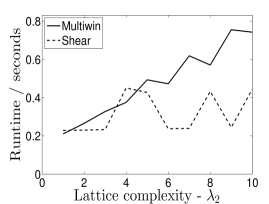
Figure 2: Computation of the DGT for nonseparable lattices with increasing lattice complexities, $\lambda_{2}$. The length is kept fixed at $L=\operatorname{lcm}\left(a,M\right)\cdot 2520$ which is the minimal legal transform length for all the tested lattices. (left) Accurate flop counts while the figures and (right) the actual running time. The Gabor system parameters are $a=32$, $M=64$ ($p/q=1/2$) (1st row), $a=40$, $M=60$ ($p/q=2/3$) (2nd row) and $a=60$, $M=80$ ($p/q=3/4$) (3rd row).

The experiments shown in Figure 2 illustrate how the computational complexity of the running time of the algorithm depends on the lattice complexity $\lambda_{2}$: The complexity of the shear algorithm is independent of $\lambda_{2}$, while the complexity of the multiwindow algorithm grows linearly.

The bumps in the curves for the multiwindow algorithm are due to variations in $q_{mw}$: The multiwindow algorithm transforms the problem into $\lambda_{2}$ different DGTs that should be computed on a lattice with redundancy $q/(p\lambda_{2})$. The number $q_{mw}$ is the nominator of this written as an irreducible fraction, and depending on $p\lambda_{2}$ it may be smaller than $q$.

The bumps in the curves for the shear algorithm are caused by whether or not a frequency side shear is required for that particular lattice configuration, and to a lesser extend whether a time-side shear is needed. As the multiwindow algorithm is faster for simple lattices, there is a cross-over point where the shear algorithm becomes faster, but the cross-over point depends strongly on the exact lattice configuration. Just considering the flop counts would predict that the cross-over happens for a smaller value of $\lambda_{2}$ that what is really the case. This is due to the fact the there are more complicated indexing operations and memory reshuffling for the shear algorithm than for the multiwindow algorithm, and this is not properly reflected in the flop count.

The cross-over point where one algorithm is faster than the other is highly dependent on the interplay between the algorithm and the computer architecture. Experience from the ATLAS [40], FFTW [19] and SPIRAL [12] projects, show that in order to have the highest performance, is it necessary to select the algorithm for a given problem size based on previous tests done on the very same machine. Performing such an optimization is beyond the scope of this paper, and we therefore cannot make statements about how to choose the most efficient cross-over points.

References

- [1] “LTFAT - The Large Time-Frequency Analysis Toolbox,” http://ltfat.sourceforge.net/.
- [2] J. Allen and L. Rabiner, “A unified approach to short-time Fourier analysis and synthesis,” Proceedings of the IEEE, vol. 65, no. 11, pp. 1558–1564, 1977.
- [3] L. Auslander, I. Gertner, and R. Tolimieri, “The discrete Zak transform application to time-frequency analysis and synthesis of nonstationary signals,” IEEE Trans. Signal Process., vol. 39, no. 4, pp. 825–835, 1991.
- [4] M. J. Bastiaans and M. C. W. Geilen, “On the discrete Gabor transform and the discrete Zak transform,” Signal Process., vol. 49, no. 3, pp. 151–166, 1996.
- [5] M. J. Bastiaans and A. J. van Leest, “From the rectangular to the quincunx Gabor lattice via fractional Fourier transformation,” Signal Processing Letters, IEEE, vol. 5, no. 8, pp. 203–205, 1998.
- [6] ——, “Modified Zak transform for the quincunx-type Gabor lattice,” in Time-Frequency and Time-Scale Analysis, 1998. Proceedings of the IEEE-SP International Symposium on. IEEE, 1998, pp. 173–176.
- [7] ——, “Gabor’s signal expansion and the gabor transform based on a non-orthogonal sampling geometry,” in Signal Processing and its Applications, Sixth International, Symposium on. 2001, vol. 1. IEEE, 2001, pp. 162–163.
- [8] ——, “Gabor’s signal expansion for a non-orthogonal sampling geometry,” Time-frequency signal analysis and processing: a comprehensive reference/Ed. B. Boashash, p. 252–260, 2003.
- [9] P. G. Casazza and M. Fickus, “Fourier transforms of finite chirps.” EURASIP J. Adv. Signal Process., vol. 2006, pp. 1–7, 2006.
- [10] O. Christensen, H. G. Feichtinger, and S. Paukner, Gabor Analysis for Imaging. Springer Berlin, 2011, vol. 3, pp. 1271–1307.
- [11] J. Cooley and J. Tukey, “An algorithm for the machine calculation of complex Fourier series,” Math. Comput, vol. 19, no. 90, pp. 297–301, 1965.
- [12] F. de Mesmay, Y. Voronenko, and M. Püschel, “Offline library adaptation using automatically generated heuristics,” in International Parallel and Distributed Processing Symposium (IPDPS), 2010.
- [13] M. Dörfler and L. D. Abreu, “An inverse problem for localization operators,” Inverse Problems, vol. 28, 2012.
- [14] H. G. Feichtinger and K. Gröchenig, “Gabor wavelets and the Heisenberg group: Gabor expansions and short time Fourier transform from the group theoretical point of view,” in Wavelets :a tutorial in theory and applications, ser. Wavelet Anal. Appl., C. K. Chui, Ed. Boston: Academic Press, 1992, vol. 2, pp. 359–397.
- [15] H. G. Feichtinger, M. Hazewinkel, N. Kaiblinger, E. Matusiak, and M. Neuhauser, “Metaplectic operators on ,” Quart. J. Math. Oxford Ser., vol. 59, no. 1, pp. 15–28, 2008.
- [16] H. G. Feichtinger and N. Kaiblinger, “2D-Gabor analysis based on 1D algorithms,” in Proc. OEAGM-97 (Hallstatt, Austria), 1997.
- [17] H. G. Feichtinger, N. Kaiblinger, and P. Prinz, “A POCS approach to Gabor analysis,” in DIP-97 (Vienna, Austria), ser. SPIE, vol. 3346, October 1997, pp. 18–29.
- [18] H. G. Feichtinger, W. Kozek, P. Prinz, and T. Strohmer, “On multidimensional non-separable Gabor expansions,” in Proc. SPIE: Wavelet Applications in Signal and Image Processing IV, August 1996.
- [19] M. Frigo and S. G. Johnson, “The design and implementation of FFTW3,” Proceedings of the IEEE, vol. 93, no. 2, pp. 216–231, 2005, special issue on "Program Generation, Optimization, and Platform Adaptation".
- [20] K. Gröchenig, Foundations of Time-Frequency Analysis. Birkhäuser, 2001.
- [21] M. Hampejs, N. Holighaus, L. Tóth, and C. Wiesmeyr, “On the subgroups of the group ,” preprint, arXiv:1211.1797, 2013.
- [22] H. Helms, “Fast Fourier transform method of computing difference equations and simulating filters,” IEEE Transactions on Audio and Electroacoustics, vol. 15, no. 2, pp. 85–90, 1967.
- [23] A. J. E. M. Janssen and P. L. Søndergaard, “Iterative algorithms to approximate canonical Gabor windows: Computational aspects,” J. Fourier Anal. Appl., vol. 13, no. 2, pp. 211–241, 2007.
- [24] S. Johnson and M. Frigo, “A Modified Split-Radix FFT With Fewer Arithmetic Operations,” IEEE Trans. Signal Process., vol. 55, no. 1, p. 111, 2007.
- [25] N. Kaiblinger, “Metaplectic representation, eigenfunctions of phase space shifts, and Gelfand-Shilov spaces for LCA groups,” Ph.D. dissertation, Dept. Mathematics, Univ. Vienna, 1999.
- [26] N. Kaiblinger and M. Neuhauser, “Metaplectic operators for finite abelian groups and ,” Indag. Math., vol. 20, no. 2, pp. 233–246, 2009.
- [27] S. Paukner, “Foundations of Gabor Analysis for Image Processing,” Master’s thesis, 2007.
- [28] M. Portnoff, “Implementation of the digital phase vocoder using the fast Fourier transform,” IEEE Trans. Acoust. Speech Signal Process., vol. 24, no. 3, pp. 243–248, 1976.
- [29] P. Prinz, “Calculating the dual Gabor window for general sampling sets,” IEEE Trans. Signal Process., vol. 44, no. 8, pp. 2078–2082, 1996.
- [30] R. Schafer and L. Rabiner, “Design and Simulation of a Speech Analysis-Synthesis System based on Short-Time Fourier Analysis,” IEEE Trans. Audio Electroac., vol. 21, no. 3, pp. 165–174, 1973.
- [31] P. L. Søndergaard, B. Torrésani, and P. Balazs, “The Linear Time Frequency Analysis Toolbox,” International Journal of Wavelets, Multiresolution Analysis and Information Processing, vol. 10, no. 4, 2012.
- [32] P. L. Søndergaard, “Efficient Algorithms for the Discrete Gabor Transform with a long FIR window,” J. Fourier Anal. Appl., vol. 18, no. 3, pp. 456–470, 2012.
- [33] T. Stockham Jr, “High-speed convolution and correlation,” in Proc. SJCC, 1966. ACM, 1966, pp. 229–233.
- [34] T. Strohmer, “Numerical algorithms for discrete Gabor expansions,” in Gabor Analysis and Algorithms. Birkhäuser, 1998, ch. 8, pp. 267–294.
- [35] T. Strohmer and S. Beaver, “Optimal OFDM system design for time-frequency dispersive channels,” IEEE Trans. Comm., vol. 51, no. 7, pp. 1111–1122, July 2003.
- [36] A. J. van Leest, “Non-separable Gabor schemes. Their Design and Implementation,” Ph.D. dissertation, Tech. Univ. Eindhoven, 2001.
- [37] A. J. van Leest and M. J. Bastiaans, “Gabor’s discrete signal expansion and the discrete Gabor transform on a non-separable lattice,” in Proc. ICASSP’00., vol. 1. IEEE, 2000, pp. 101–104.
- [38] ——, “Implementations of non-separable Gabor schemes,” in Proc. EUSIPCO 2004 ,Vienna,Austria,, 2004, pp. 1565–1568.
- [39] A. Weil, “Sur certains groupes d’opérateurs unitaires,” Acta Math., vol. 111, pp. 143–211, 1964.
- [40] R. C. Whaley and A. Petitet, “Minimizing development and maintenance costs in supporting persistently optimized BLAS,” Software: Practice and Experience, vol. 35, no. 2, pp. 101–121, February 2005.
- [41] Y. Y. Zeevi and M. Zibulski, “Oversampling in the Gabor scheme,” IEEE Trans. Signal Process., vol. 41, no. 8, pp. 2679–2687, 1993.
- [42] M. Zibulski and Y. Y. Zeevi, “Signal- and image-component separation by a multi-window Gabor-type scheme,” in Proc. ICPR, 1996, vol. 2. Vienna , Austria, pp. 835 –839.
- [43] ——, “Analysis of multiwindow Gabor-type schemes by frame methods,” Appl. Comput. Harmon. Anal., vol. 4, no. 2, pp. 188–221, 1997.
- [44] ——, “Discrete multiwindow Gabor-type transforms.” IEEE Trans. Signal Process., vol. 45, no. 6, pp. 1428–1442, 1997.
- [45] ——, “The generalized Gabor scheme and its application in signal and image representation,” in Signal and Image Representation in Combined Spaces, ser. Wavelet Anal. Appl. Academic Press, 1998, vol. 7, pp. 121–164.