Abrupt transition in the structural formation of interconnected networks

Abstract

Our current world is linked by a complex mesh of networks where information, people and goods flow. These networks are interdependent each other, and present structural and dynamical features different from those observed in isolated networks. While examples of such “dissimilar” properties are becoming more abundant, for example diffusion, robustness and competition, it is not yet clear where these differences are rooted in. Here we show that the composition of independent networks into an interconnected network of networks undergoes a structurally sharp transition as the interconnections are formed. Depending of the relative importance of inter and intra-layer connections, we find that the entire interdependent system can be tuned between two regimes: in one regime, the various layers are structurally decoupled and they act as independent entities; in the other regime, network layers are indistinguishable and the whole system behave as a single-level network. We analytically show that the transition between the two regimes is discontinuous even for finite size networks. Thus, any real-world interconnected system is potentially at risk of abrupt changes in its structure that may reflect in new dynamical properties.

Interacting, interdependent or multiplex networks are different ways of naming the same class of complex systems where networks are not considered as isolated entities but interacting each other. In multiplex, the nodes at each network are instances of the same entity, thus the networks are representing simply different categorical relationships between entities, and usually categories are represented by layers. Interdependent networks is a more general framework where nodes can be different at each network.
Many, if not all, real networks are “coupled” with other real networks. Examples can be found in several domains: social networks (e.g., Facebook, Twitter, etc.) are coupled because they share the same actors lamb ; multimodal transportation networks are composed of different layers (e.g., bus, subway, etc.) that share the same locations barth ; the functioning of communication and power grid systems depend one on the other buldy . So far, all phenomena that have been studied on interdependent networks, including percolation buldy ; grass , epidemics mendiola , and linear dynamical systems gomez , have provided results that differ much from those valid in the case of isolated complex networks. Sometimes the difference is radical: for example, while isolated scale-free networks are robust against failures of their nodes or edges jeong , scale-free interdependent networks are instead very fragile buldy ; grass .
Given such observations, two fundamentally important theoretical questions are in order: (i) Why do dynamical and critical phenomena running on interdependent network models differ so much from their analogous in isolated networks?; (ii) What are the regimes of applicability of the theory valid for isolated networks to interdependent networks? In this paper, we provide an analytic answer to both these questions by characterizing the structural properties of the whole interconnected network in terms of the networks that compose it.

Figure 1: a) Schematic example of two interdependent networks $A$ and $B$. In this representation, nodes of the same color are one-to-one interdependent. b) In our model, inter-layer edges have weights equal to $p$.

For simplicity, we consider here the case of two interdependent networks. The following method can be, however, generalized to an arbitrary number of interdependent networks and its solution is reported in the Supplementary Information. We assume that the two interdependent networks $A$ and $B$ are undirected and weighted, and that they have the same number of nodes $N$. The weighted adjacency matrices of the two graphs are indicated as $A$ and $B$, respectively, and they have both dimensions $N\times N$. With this notation, the element $A_{ij}=A_{ji}$ is equal to the weight of the connection between the nodes $i$ and $j$ in network $A$. The definition of $B$ is analogous.
We consider the case of one-to-one symmetric interdependency buldy between nodes in the networks $A$ and $B$ (see Fig. 1A). In the more general case of multiple interdependencies, the solution is analogous and reported in the Supplementary Information. The connections between interdependent nodes of the two networks are weighted by a factor $p$ (see Fig. 1B), any other weighted factor for the networks $A$ and $B$ is implicitly absorbed in their weights. The supra-adjacency matrix $G$ of the whole network is therefore given by

$$G=\left(\begin{array}[]{cc}A&p\mathbbm{1}\\ p\mathbbm{1}&B\end{array}\right)\,,$$ (1)

where $\mathbbm{1}$ is the identity matrix of dimensions $N\times N$.
Using this notation we can define the supra-laplacian of the interconnected network as

$$\mathcal{L}=\left(\begin{array}[]{cc}\mathcal{L}_{A}+p\mathbbm{1}&-p\mathbbm{1}\\ -p\mathbbm{1}&\mathcal{L}_{B}+p\mathbbm{1}\end{array}\right)\,.$$ (2)

The blocks present in $\mathcal{L}$ are square symmetric matrices of dimensions $N\times N$, In particular, $\mathcal{L}_{A}$ and $\mathcal{L}_{B}$ are the laplacians of the networks $A$ and $B$, respectively.
Our investigation focus on the analysis of the spectrum of the supra-Laplacian to ascertain the origin of the structural changes of the merging of networks in an interconnected system. The spectrum of the laplacian of a graph is a fundamental mathematical object for the study of the structural properties of the graph itself. There are many applications and results on graph Laplacian eigenpairs and their relations to numerous graph invariants (including connectivity, expanding properties, genus, diameter, mean distance, and chromatic number) as well as to partition problems (graph bisection, connectivity and separation, isoperimetric numbers, maximum cut, clustering, graph partition), and approximations for optimization problems on graphs (cutwidth, bandwidth, min-p-sum problems, ranking, scaling, quadratic assignment problem) merris ; chungbook ; eigbook ; chung .
Note that, for any graph, all eigenvalues of its laplacian are non negative numbers. The smallest eigenvalue is always equal to zero and the eigenvector associated to it is trivially a vector whose entries are all identical. The second smallest eigenvalue $\lambda_{2}$ also called the algebraic connectivity fiedler1 is one of the most significant eigenvalues of the Laplacian. It is strictly larger than zero only if the graph is connected. More importantly, the eigenvector associated to $\lambda_{2}$, which is called the characteristic valuation or Fiedler vector of a graph, provides even deeper about its structure fiedler2 ; fiedler3 ; mohar . For example, the components of this vector associated to the various nodes of the network are used in spectral clustering algorithms for the bisection of graphs clustering .

Our approach consists in the study of the behavior of the second smallest eigenvalue of the supra-laplacian matrix $\mathcal{L}$ and its characteristic valuation as a function of $p$, given the single-layer network laplacians $\mathcal{L}_{A}$ and $\mathcal{L}_{B}$.
According to the theorem by Courant and Fisher (i.e., the so-called min-max principle) courant ; fisher , the second smallest eigenvalue of $\mathcal{L}$ is given by

$$\lambda_{2}\left(\mathcal{L}\right)=\min_{\left|v\right>\in\mathcal{V}}\,\left<v\right|\mathcal{L}\left|v\right>\;,$$ (3)

where $\left|v\right>\in\mathcal{V}\,\textrm{ is such that }\,\left<v|1\right>=0,\left<v|v\right>=1$.
The vector $\left|1\right>$ has $2N$ entries all equal to $1$. Eq. (3) means that $\lambda_{2}\left(\mathcal{L}\right)$ is equal to the minimum of the function $\left<v\right|\mathcal{L}\left|v\right>$, over all possible vectors $\left|v\right>$ that are orthogonal to the vector $\left|1\right>$ and that have norm equal to one. The vector for which such minimum is reached is thus the characteristic valuation of the supra-laplacian (i.e., $\mathcal{L}\left|v\right>=\lambda_{2}\left|v\right>$).
We distinguish two blocks of size $N$ in the vector $\left|v\right>$ by writing it as $\left|v\right>=\left|v_{A},v_{B}\right>$. In this notation, $\left|v_{A}\right>$ is the part of the eigenvector whose components corresponds to the nodes of network $A$, while $\left|v_{B}\right>$ is the part of the eigenvector whose components corresponds to the nodes of network $B$. We can now write

$$\begin{array}[]{ll}\left<v\right|\mathcal{L}\left|v\right>=&\left<v_{A},v_{B}\right|\mathcal{L}\left|v_{A},v_{B}\right>=\\ &\left<v_{A}\right|\mathcal{L}_{A}\left|v_{A}\right>+\left<v_{B}\right|\mathcal{L}_{B}\left|v_{B}\right>+\\ &p\left(\left<v_{A}|v_{A}\right>+\left<v_{B}|v_{B}\right>-2\left<v_{A}|v_{B}\right>\right)\end{array}$$

and the previous set of constraints as $\left<v_{A}|1\right>+\left<v_{B}|1\right>=0$ and $\left<v_{A}|v_{A}\right>+\left<v_{B}|v_{B}\right>=1$, where now all vectors have dimension $N$. Accounting for such constraints, we can finally rewrite the minimization problem as

$$\begin{array}[]{l}\lambda_{2}\left(\mathcal{L}\right)=p+\min_{\left|v\right>\in\mathcal{V}}\,\left\{\left<v_{A}\right|\mathcal{L}_{A}\left|v_{A}\right>\right.\\ \left.+\left<v_{B}\right|\mathcal{L}_{B}\left|v_{B}\right>-2p\left<v_{A}|v_{B}\right>\right\}\end{array}\;.$$ (4)

This minimization problem can be solved using Lagrange multipliers (see Supplementary Information for technical details).
In this way we are able to find that the second smallest eigenvalue of the supra-laplacian matrix $\mathcal{L}$ is given by

$$\lambda_{2}\left(\mathcal{L}\right)=\left\{\begin{array}[]{ll}2p&\textrm{ , if }p\leq p^{*}\\ \leq\frac{1}{2}\lambda_{2}\left(\mathcal{L}_{A}+\mathcal{L}_{B}\right)&\textrm{ , if }p\geq p^{*}\end{array}\right.\;.$$ (5)

Thus indicating that the algebraic connectivity of the interconnected system follows two distinct regimes, one in which its value is independent of the structure of the two layers, and the other in which its upper bound is limited by the algebraic connectivity of the weighted superposition of the two layers whose laplacian is given by $\frac{1}{2}\left(\mathcal{L}_{A}+\mathcal{L}_{B}\right)$. More importantly, the discontinuity in the first derivative of $\lambda_{2}$ is reflected in a radical change of the structural properties of the system happening at $p^{*}$ (see Supplementary Information). Such dramatic change is visible in the coordinates of characteristic valuation of the nodes of the two network layers. In the regime $p\leq p^{*}$, the components of the eigenvector are

$$\left|v_{A}\right>=-\left|v_{B}\right>\qquad\textrm{ where }\left|v_{A}\right>=\pm\frac{1}{\sqrt{2N}}\left|1\right>\;.$$ (6)

This means that the two network layers are structurally disconnected and independent. For $p\geq p^{*}$, we have

$$\left<v_{A}|1\right>=\left<v_{B}|1\right>=0\;,$$ (7)

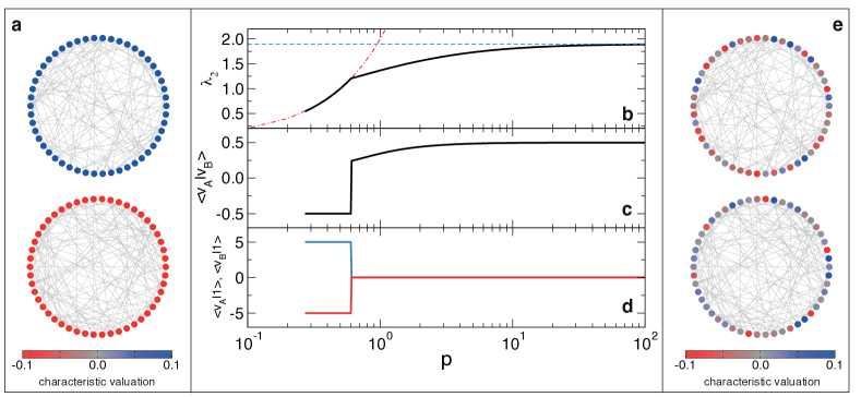
Figure 2: Algebraic connectivity and Fiedler vector for two interdependent Erdős-Rényi networks of $N=50$ nodes and average degree $\bar{k}=5$. In this example, the critical point is $p^{*}=0.602(1)$. a) Characteristic valuation of the nodes in the two network layers for $p=0.602$. b) Algebraic connectivity of the system (black line). The discontinuity of the first derivative of $\lambda_{2}$ is very clear. The two different regimes $2p$ and $\frac{\lambda_{2}\left(\mathcal{L}_{A}+\mathcal{L}_{B}\right)}{2}$ are shown as red dot-dashed and blue dashed lines, respectively. c) Inner product $\left<v_{A}|v_{B}\right>$ between the part of the Fiedler eigenvector ($\left|v_{A}\right>$) corresponding to nodes in the network $A$ and the one ($\left|v_{B}\right>$) corresponding to vertices in network $B$ as a function of $p$. d) Inner products $\left<v_{A}|1\right>$ and $\left<v_{B}|1\right>$ as functions of $p$. $\left<v_{A}|1\right>$ and $\left<v_{B}|1\right>$ indicate the sum of all components of the Fiedler vectors $\left|v_{A}\right>$ and $\left|v_{B}\right>$, respectively. e) Characteristic valuation of the nodes in the two network layers for $p=0.603$.

which means that the components of the vector corresponding to interdependent nodes of network $A$ and $B$ have the same sign, while nodes in the same layer have alternating signs. Thus in this second regime, the system connectivity is dominated by inter-layer connections, and the two network layers are structurally indistinguishable.
The critical value $p^{*}$ at which the transition occurs is the point at which we observe the crossing between the two different behaviors of $\lambda_{2}$, which means

$$p^{*}\leq\frac{1}{4}\,\lambda_{2}\left(\mathcal{L}_{A}+\mathcal{L}_{B}\right)\;.$$ (8)

This upper bound becomes exact in the case of identical network layers (see Supplementary Information). Since inter-layer connections have weights that grows with $p$, the transition happens at the point at which the weight of the inter-layer connections exceeds the half part of the inverse of the algebraic connectivity of the weighted super-position of both network layers (see Fig. 2). In the case of $\ell$ network layers, the result is equivalent to the superposition of all of them (see Supplementary Information).
It is important to notice that the discontinuity in the first derivative of $\lambda_{2}\left(\mathcal{L}\right)$ can be interpreted as the consequence of the crossing of two different populations of eigenvalues (see the case of identical layers in the Supplementary Information). The same crossing will also happen for the other eigenpairs of the graph laplacian (except for the smallest and the largest ones), and thus will reflect in the discontinuities in the first derivatives of the corresponding eigenvalues.

A physical interpretation of the algebraic phase transition that we are able to analytically predict can be given by viewing the function $\left<v\right|\mathcal{L}\left|v\right>$ as an energy-like function. From this point of view, Eq. (3) becomes equivalent to a search for the ground state energy, and the characteristic valuation can be viewed as the ground state configuration. Such analogy is straightforward if one realizes that Eq. (3) is equivalent to the minimization of the weighted cut of the entire networked system [whose adjacency matrix $G$ is defined in Eq. (1)], and that the minimum of this function corresponds to the ground state of a wide class of energy functions kolmo and fitness landscapes land . These include, among others, the energy associated to the Ising spin models parisi and costs functions of combinatorial optimization problems, such as the traveling salesman problem sale . In summary, the structural transition of interdependent networks involves a discontinuity in the first derivative of an energy-like function, and thus, according to the Ehrenfest classification of phase transitions, it is a discontinuous transition phase .
Since the transition at the algebraic level has the same nature as the connectivity transition that has been studied by Buldyrev et al. in the same class of networked systems buldy , it is worth to discuss about the relations between the two phase transitions. We can reduce our model to the annealed version of the model considered by Buldyrev et al. by setting $A=t^{2}A$, $B=t^{2}B$ and $p=t$, being $1-t$ the probability that one node in one of the networks fails. All the results stated so far hold, with only two different interpretations. First, the upper bound of Eq. (8) becomes a lower bound for the critical threshold of the algebraic transition that reads in terms of occupation probability as

$$t_{c}\geq\frac{4}{\lambda_{2}\left(\mathcal{L}_{A}+\mathcal{L}_{B}\right)}\;.$$ (9)

Second, the way to look at the transition must be reversed: network layers are structurally independent (i.e., the analogous of the non percolating phase) for values of $t\leq t_{c}$, while become algebraically connected (i.e., analogous of the percolating phase) when $t\geq t_{c}$.
As it is well known, the algebraic connectivity represents a lower bound for both the edge connectivity and node connectivity of graph (i.e., respectively the minimal number of edges or nodes that should be removed to disconnect the graph) fiedler1 . Indeed, the algebraic connectivity of a graph is often used as a control parameter to make the graph more resilient to random failures of its nodes or edges jama . Thus, the lower bound of Eq. (9) represents also a lower bound for the critical percolation threshold measured by Buldyrev et al. Interestingly, our prediction turns out to be a sharp estimate of the lower bound.
For the Erdős-Rényi model, we have in fact $t_{c}\geq 2/\bar{k}$, if the two networks have the same average degree $\bar{k}$, and this value must be compared with $2.455/\bar{k}$ as predicted by Buldyrev et al. buldy ; grass . Similarly, we are able to predict that $t_{c}$ grows as the degree distribution of the network becomes more broad chung , in the same way as it has been numerically observed by Buldyrev et al. buldy .
Although we are not able to directly map the algebraic transition to the percolation one, we believe that the existence of a first-order transition at the algebraic level represents an indirect support of the discontinuity of the percolation transition.

In conclusion, we have provided the exact analytic treatment of the structural properties of interconnected networks. We have presented the exact solution for the algebraic connectivity of these network models. For simplicity, we have considered the simplest case of one-to-one interdependency but our formalism can be easily extended to study more complicated dependence relationships among the nodes of the different layers. Our proof does not rely on any approximation but on a very intuitive mathematical approach.
The structural phase transitions in interdependent networks are first-order in nature. This differentiate multi- and single-level networks in a radical manner. We remark that the discontinuity in the first derivative of the algebraic connectivity affects directly a vast class of systems whose dynamics is driven by the minimization of energy-like functions associated to the structure of the system, but the same conclusions can be also extended to other critical phenomena whose features depend on the third, fourth, etc. smallest eigenpairs of the graph laplacian.
Moreover, the point at which we observe the discontinuity in the first derivative of the algebraic connectivity (but also on other eigenvalues of the graph laplacian) defines a clear scale for the applicability of the results valid for isolated networks. In one case, network layers can be considered as independent, in the other case the entire system can be considered as a single-level network. The fact that the transition between the two regimes is so sharp leaves out only a very tiny interval of interaction values where it makes sense to consider the system as composed of many interacting network layers.
Our results have also deep practical implications. The abrupt nature of the structural transition is not only visible in the limit of infinitely large systems, but for networks of any size. Thus, even real networked systems composed of few elements may be subjected to abrupt structural changes, including failures. Our theory provides, however, fundamental aids for the prevention of such collapses. It allows, in fact, not only the prediction of the critical point of the transition, but, more importantly, to accurately design the structure of such systems in order to make them more robust. For example, the percolation threshold of interconnected systems can be simply decreased by increasing the algebraic connectivity of the superposition of the network layers. This means that an effective strategy to make an interdependent system more robust is to avoid the repetition of edges among layers, and thus bring the superposition of the layers as close as possible to an all-to-all topology.

Supplementary Information

Solution of the algebraic connectivity value of interconnected networks

In the following, we will make use of the standard bra-ket notation for vectors. In this notation, $\left|x\right>$ indicates a column vector, $\left<x\right|$ indicates the transposed (i.e., row vector) of $\left|x\right>$, $\left<x|y\right>=\left<y|x\right>$ indicates the inner product between the vectors $\left|x\right>$ and $\left|y\right>$, $A\left|x\right>$ indicates the action of matrix $A$ on the column vector $\left|x\right>$, and $\left<x\right|A$ indicates the action of matrix $A$ on the row vector $\left<x\right|$.

First of all, we can simply state that for the algebraic connectivity of Eq. (4) we must have that

$$\lambda_{2}\left(\mathcal{L}\right)\leq\frac{1}{2}\lambda_{2}\left(\mathcal{L}_{A}+\mathcal{L}_{B}\right)\;,$$ (S1)

where this upper bound comes out directly from the definition of the minimum of a function. For every $\mathcal{Q}\subseteq\mathcal{V}$, we have in fact that

$$\min_{\left|v\right>\in\mathcal{V}}\left<v\right|\mathcal{L}\left|v\right>\leq\min_{\left|v\right>\in\mathcal{Q}}\left<v\right|\mathcal{L}\left|v\right>$$

simply because we are restricting the domain in which finding the minimum of the function $\left<v\right|\mathcal{L}\left|v\right>$. The particular value of the upper bound of Eq. (S1) is then given by setting $\mathcal{Q}$ as

$$\begin{array}[]{l}\left|v\right>=\left|v_{A},v_{B}\right>\in\mathcal{Q}\,\textrm{ is such that }\,\left|v_{A}\right>=\left|v_{B}\right>=\left|q\right>\\ \textrm{ , with }\left<q|1\right>=0,\left<q|q\right>=1/2\end{array}\;.$$

To find the minimum of the function expressed in Eq. (4), we use the Lagrange multipliers’ formalism. This means finding the minimum of the function

$$\begin{array}[]{ll}M=&\left<v_{A}\right|\mathcal{L}_{A}\left|v_{A}\right>+\left<v_{B}\right|\mathcal{L}_{B}\left|v_{B}\right>-2p\left<v_{A}|v_{B}\right>\\ &-r\left(\left<v_{A}|1\right>+\left<v_{B}|1\right>\right)-s\left(\left<v_{A}|v_{A}\right>+\left<v_{B}|v_{B}\right>-1\right)\end{array}\;,$$

where the constraints of the minimization problem have been explicitly inserted in the function to minimize through the Lagrange multipliers $r$ and $s$. In the following calculations, we will make use of the identities

$$\begin{array}[]{l}\frac{\partial\,}{\partial\,\left|x\right>}\left<t|x\right>=\frac{\partial\,}{\partial\,\left|x\right>}\left<x|t\right>=\left<t\right|\\ \frac{\partial\,}{\partial\,\left|x\right>}\left<x|x\right>=2\left<x\right|\\ \frac{\partial\,}{\partial\,\left|x\right>}\left<x\right|A\left|x\right>=2\left<x\right|A\textrm{, if }A=A^{T}\end{array}\;,$$

where $\frac{\partial\,}{\partial\,\left|x\right>}$ indicates the derivative with respect to all the coordinates of the vector $\left|x\right>$. Equating to zero the derivatives of $M$ with respect to $r$ and $s$, we obtain the constraints that we imposed. By equating to zero the derivative of $M$ with respect to $\left|v_{A}\right>$, we obtain instead

$$\frac{\partial\,M}{\partial\,\left|v_{A}\right>}=2\left<v_{A}\right|\mathcal{L}_{A}-2p\left<v_{B}\right|-r\left<1\right|-2s\left<v_{A}\right|=\left<0\right|\;,$$ (S2)

and, similarly for the derivative of $M$ with respect to $\left|v_{B}\right>$,we obtain

$$\frac{\partial\,M}{\partial\,\left|v_{B}\right>}=2\left<v_{B}\right|\mathcal{L}_{B}-2p\left<v_{A}\right|-r\left<1\right|-2s\left<v_{B}\right|=\left<0\right|\;.$$ (S3)

Multiplying both equations for $\left|1\right>$, we have $2\left<v_{A}\right|\mathcal{L}_{A}\left|1\right>-2p\left<v_{B}|1\right>-r\left<1|1\right>-2s\left<v_{A}|1\right>=0$ and $2\left<v_{B}\right|\mathcal{L}_{B}\left|1\right>-2p\left<v_{A}|1\right>-r\left<1|1\right>-2s\left<v_{B}|1\right>=0$, that can be simplified in $2(p-s)\left<v_{A}|1\right>-rN=0$ and $2(p-s)\left<v_{B}|1\right>-rN=0$ because $\mathcal{L}_{A}\left|1\right>=\mathcal{L}_{B}\left|1\right>=\left|0\right>$ and $\left<v_{A}|1\right>=-\left<v_{B}|1\right>$. Summing them, we obtain $r=0$. Finally, we can write

$$\begin{array}[]{l}(p-s)\left<v_{A}|1\right>=0\\ (p-s)\left<v_{B}|1\right>=0\end{array}\;.$$ (S4)

These equations can be true in two cases: (i) $\left<v_{A}|1\right>\neq 0$ or $\left<v_{B}|1\right>\neq 0$ and $s=p$; (ii) $\left<v_{A}|1\right>=\left<v_{B}|1\right>=0$. In the following, we analyze these two cases separately.

First, let us suppose that $s=p$, and that at least one of the two equations $\left<v_{A}|1\right>\neq 0$ and $\left<v_{B}|1\right>\neq 0$ is true. If we set $s=p$ in Eqs. (S2) and (S3), they become

$$\left<v_{A}\right|\mathcal{L}_{A}-p\left<v_{B}\right|-p\left<v_{A}\right|=\left<0\right|$$ (S5)

and

$$\left<v_{B}\right|\mathcal{L}_{B}-p\left<v_{A}\right|-p\left<v_{B}\right|=\left<0\right|\;.$$ (S6)

If we multiply the first equation for $\left|v_{A}\right>$ and the second equation for $\left|v_{B}\right>$, the sum of these two new equations is

$$\left<v_{A}\right|\mathcal{L}_{A}\left|v_{A}\right>+\left<v_{B}\right|\mathcal{L}_{B}\left|v_{B}\right>-2p\left<v_{A}|v_{B}\right>=p\;.$$ (S7)

If we finally insert this expression in Eq. (4), we find that the second smallest eigenvalue of the supra-laplacian is

$$\lambda_{2}\left(\mathcal{L}\right)=2p\;.$$ (S8)

We can further determine the components of Fiedler vector in this regime. If we take the difference between Eqs. (S5) and (S6), we have $\left<v_{A}\right|\mathcal{L}_{A}=\left<v_{B}\right|\mathcal{L}_{B}$. On the other hand, Eq. (S8) is telling us that $\left<v_{A}\right|\mathcal{L}_{A}\left|v_{A}\right>=-\left<v_{B}\right|\mathcal{L}_{B}\left|v_{B}\right>$ because the only term surviving in Eq. (S7) is the one that depends on $p$. Since $\left<v_{A}\right|\mathcal{L}_{A}\left|v_{A}\right>$ ($\left<v_{B}\right|\mathcal{L}_{B}\left|v_{B}\right>$) is always larger than zero, unless $\left|v_{A}\right>=c\left|1\right>$ ($\left|v_{B}\right>=c\left|1\right>$), with $c$ arbitrary constant value, we obtain Eq. (6). Thus in this regime, both the relations $\left<v_{A}|1\right>\neq 0$ and $\left<v_{B}|1\right>\neq 0$ must be simultaneously true. Eq. (6) also means that $\left<v_{A}|v_{B}\right>=-\frac{1}{2}$.

The other possibility is that Eqs. (S4) are satisfied because $\left<v_{A}|1\right>=0$ and $\left<v_{B}|1\right>=0$ are simultaneously true. In this case, the average value of the components of the vectors $\left|v_{A}\right>$ and $\left|v_{B}\right>$ is zero, and thus the coordinates of the Fiedler vector corresponding to the nodes of the same layer have alternatively negative and positive signs. More can be said in the case of identical layers, where the problem can be solved exactly (see next section). In this case, the upper bound of Eq. (S1) becomes the exact solution for the algebraic connectivity and reads as $\lambda_{2}\left(\mathcal{L}\right)=\lambda_{2}\left(\mathcal{M}\right)$, with $\mathcal{M}$ laplacian of both layers. More importantly, the Fiedler vector satisfies the relation

$$\left|v_{A}\right>=\left|v_{B}\right>\;.$$ (S9)

The same relation does not hold in general for different network layers, although the coordinates of the Fiedler vector of two interdependent nodes seem to have the same sign.

Spectrum of the laplacian for two identical network layers

Consider the case $\mathcal{L}_{A}=\mathcal{L}_{B}=\mathcal{M}$. Finding the eigenvalues of the supra-laplacian $\mathcal{L}$ means finding the solutions of the eigenvalue problem

$$\textrm{det}\left(\mathcal{L}-\lambda\mathbbm{1}\right)=0\;.$$

Let us write the eigenvalues $\lambda$ as functions of the eigenvalues $\mu$ of $\mathcal{M}$. This can be done in the following way.

$$\left(\mathcal{L}-\lambda\mathbbm{1}\right)=\left(\begin{array}[]{cc}\mathcal{M}+p\mathbbm{1}-\lambda\mathbbm{1}&-p\mathbbm{1}\\ -p\mathbbm{1}&\mathcal{M}+p\mathbbm{1}-\lambda\mathbbm{1}\end{array}\right)$$

Consider the matrices

$$U=\left(\begin{array}[]{cc}Q&\emptyset\\ \emptyset&Q\end{array}\right)$$

$$U^{T}=\left(\begin{array}[]{cc}Q^{T}&\emptyset\\ \emptyset&Q^{T}\end{array}\right)\;,$$

with $Q^{T}\mathcal{M}Q=D$ and $D$ diagonal matrix containing the eigenvalues $\mu$ of $\mathcal{M}$, so that $Q^{T}Q=QQ^{T}=\mathbbm{1}$, and the matrices

$$V=\frac{1}{\sqrt{2}}\left(\begin{array}[]{cc}\mathbbm{1}&-\mathbbm{1}\\ \mathbbm{1}&\mathbbm{1}\end{array}\right)$$

$$V^{T}=\frac{1}{\sqrt{2}}\left(\begin{array}[]{cc}\mathbbm{1}&\mathbbm{1}\\ -\mathbbm{1}&\mathbbm{1}\end{array}\right)$$

We can write

$$\begin{array}[]{l}V^{T}U^{T}\left(\mathcal{L}-\lambda\,\mathbbm{1}\right)UV=\\ V^{T}\left(\begin{array}[]{cc}D+p\mathbbm{1}-\lambda\mathbbm{1}&-p\mathbbm{1}\\ -p\mathbbm{1}&D+p\mathbbm{1}-\lambda\mathbbm{1}\end{array}\right)V\end{array}$$

$$\begin{array}[]{l}V^{T}U^{T}\left(\mathcal{L}-\lambda\,\mathbbm{1}\right)UV=\\ \frac{1}{\sqrt{2}}\left(\begin{array}[]{cc}D-\lambda\mathbbm{1}&D-\lambda\mathbbm{1}\\ -D+\lambda\mathbbm{1}-2p\mathbbm{1}&D-\lambda\mathbbm{1}+2p\mathbbm{1}\end{array}\right)V\end{array}$$

$$\begin{array}[]{l}V^{T}U^{T}\left(\mathcal{L}-\lambda\,\mathbbm{1}\right)UV=\\ \frac{1}{2}\left(\begin{array}[]{cc}2D-2\lambda\mathbbm{1}&\emptyset\\ \emptyset&2D-2\lambda\mathbbm{1}+4p\mathbbm{1}\end{array}\right)\end{array}\;.$$

Since

$$\textrm{det}\left(\mathcal{L}-\lambda\mathbbm{1}\right)=\textrm{det}\left[V^{T}U^{T}\left(\mathcal{L}-\lambda\mathbbm{1}\right)UV\right]\;,$$

the eigenvalues of the supra-laplacian $\mathcal{L}$ are given by $\{\mu\}$ and $\{\mu+2p\}$, where $\left\{\mu\right\}$ are the eigenvalues of the single layer laplacian $\mathcal{M}$.
This means that there two possible candidates for $\lambda_{2}\left(\mathcal{L}\right)$: $\mu_{2}$ and $2p$. The equation that delimits the different regions is thus

$$\mu_{2}\left(\mathcal{M}\right)=2p\;.$$

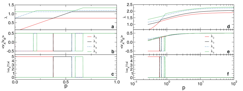
Figure S1: Properties of some eigenpairs of the supra-laplacian matrix for two interdependent Erdős-Rényi networks of $N=50$ nodes and average degree $\bar{k}=5$. The networks used in this plot are the same as those considered in Fig. 2. In panels a, b and c, we used identical layers (only network $A$ for both layers), in panels d, e and f, we used instead different network layers. a) and d) Eigenvalues $\lambda_{k}$, with $k=2,3,4$ and $5$ as functions of $p$. b) and e) Inner product $\left<v_{A}|v_{B}\right>$ between the part of the eigenvector ($\left|v_{A}\right>$) corresponding to nodes in the network $A$ and the one ($\left|v_{B}\right>$) corresponding to vertices in network $B$ as a function of $p$. c) and f) Absolute value of the inner product $\left<v_{A}|1\right>$ as a function of $p$.

Please note that a similar behavior is valid also for the other eigenvalues of the laplacian (except the largest and the smallest, see Fig. S1). For example, the third smallest eigenvalue $\lambda_{3}$ of the supra-laplacian exhibits three different behaviors, an its derivative is discontinuous at two values of $p$ identified by the equations

$$\mu_{2}\left(\mathcal{M}\right)=2p$$

(i.e., the same point in which the first derivative of $\lambda_{2}$ is discontinuous) and

$$\mu_{3}\left(\mathcal{M}\right)=\mu_{2}\left(\mathcal{M}\right)+2p\;.$$

The behavior of the other eigenvalues is even richer, and in principle several discontinuity points are present. A similar behavior is also present in the case of different network layers (see Fig. S1).

Spectrum of the laplacian with arbitrary number of identical interconnected networks

The same result holds also for more than two identical interdependent networks. In that case, the matrix $V$ is the block matrix able to diagonalize the block matrix composed of $\ell$ blocks equal to the identity matrix. $U$ is still the matrix able to diagonalize the laplacian $\mathcal{M}$. The resulting matrix, after the similarity transformation

$$V^{T}U^{T}\left(\mathcal{L}-\lambda\mathbbm{1}\right)UV$$

has one block diagonal element equal to $D+\ell\,p\mathbbm{1}-\lambda\mathbbm{1}$, and the remaining $\ell-1$ block diagonal elements proportional to $D-\lambda\mathbbm{1}$. The eigenvalues of the supra-laplacian matrix are thus $\{\mu\}$ with multiplicity $\ell-1$, and $\{\mu+\ell p\}$ with multiplicity one. We thus have still two regimes for the second smallest eigenvalue given by

$$\lambda_{2}\left(\mathcal{L}\right)=\left\{\begin{array}[]{ll}\ell p&\textrm{ , if }p\leq p^{*}\\ \mu_{2}\left(\mathcal{M}\right)&\textrm{ , if }p\geq p^{*}\end{array}\right.\;,$$

where $p^{*}$ is given by

$$p^{*}=\frac{1}{\ell}\mu_{2}\left(\mathcal{M}\right)\;.$$

General case with arbitrary number of interconnected networks

Let us consider the case of $\ell$ different layers. The supra-laplacian matrix is composed of $\ell\times\ell$ block matrices of dimensions $N\times N$. Along the diagonal, we have

$$\mathcal{L}_{mm}=\mathcal{L}_{m}+(\ell-1)p\mathbbm{1}$$

while on the off-diagonal blocks we have

$$\mathcal{L}_{mn}=-p\mathbbm{1}\;,$$

where $\mathcal{L}_{m}$ is the laplacian matrix of the layer $m$, while $\mathbbm{1}$ is the identity matrix. Let us write the generic vector as

$$\left|v\right>=\left|v_{1},v_{2},\ldots,v_{\ell}\right>\;.$$

Then

$$\begin{array}[]{l}\left<v\right|\mathcal{L}\left|v\right>=\sum_{m}\left<v_{m}\right|\mathcal{L}_{m}\left|v_{m}\right>\\ +(\ell-1)p\sum_{m}\left<v_{m}|v_{m}\right>-p\sum_{m}\sum_{n\neq m}\left<v_{m}|v_{n}\right>\end{array}\;.$$

For the Courant-Fisher min-max theorem, the second smallest eigenvalue $\lambda_{2}\left(\mathcal{L}\right)$ of the supra-laplacian matrix is given by

$$0\leq\lambda_{2}\left(\mathcal{L}\right)=\min_{\mathcal{V}}\left<v\right|\mathcal{L}\left|v\right>\;,$$

with

$$\begin{array}[]{l}\left|v\right>\in\mathcal{V}\textrm{ is such that }\\ \left|v\right>\neq\left|0\right>,\left<v|v\right>=1\textrm{ and }\left<v|1\right>=0\end{array}\;.$$

$\left|1\right>$ is the column vector whose $\ell N$ entries are equal to one, while $\left|0\right>$ is the column vector whose $\ell N$ entries are equal to zero. The constraints of the vectors in $\mathcal{V}$ can be written also as

$$\left<v|v\right>=\sum_{m}\left<v_{m}|v_{m}\right>=1\;\textrm{ and }\;\left<v|1\right>=\sum_{m}\left<v_{m}|1\right>=0\;,$$

where $\left|1\right>$ now indicates a column vector whose $N$ entries are equal to one, and $\left|0\right>$ now indicates a column vector whose $N$ entries are equal to zero. Imposing the constraint $\sum_{m}\left<v_{m}|v_{m}\right>=1$, the former expression reduces to

$$\begin{array}[]{l}\left<v\right|\mathcal{L}\left|v\right>=\sum_{m}\left<v_{m}\right|\mathcal{L}_{m}\left|v_{m}\right>\\ -p\sum_{m}\sum_{n\neq m}\left<v_{m}|v_{n}\right>+(\ell-1)p\end{array}\;.$$ (S10)

First of all, we can easily set an upper bound for $\lambda_{2}\left(\mathcal{L}\right)$ by simply reducing the set of vectors where searching for the minimum of the function $\left<v\right|\mathcal{L}\left|v\right>$. For all $\mathcal{Q}\subseteq\mathcal{S}$, the definition of minimum implies that

$$\begin{array}[]{l}\lambda_{2}\left(\mathcal{L}\right)\leq\min_{\mathcal{Q}}\,\left<v\right|\mathcal{L}\left|v\right>=(\ell-1)p\\ +\,\min_{\mathcal{Q}}\,\left[\sum_{m}\left<v_{m}\right|\mathcal{L}_{m}\left|v_{m}\right>-p\sum_{m}\sum_{n\neq m}\left<v_{n}|v_{m}\right>\right]\end{array}\;.$$

In particular, if we choose $\mathcal{Q}$

$$\begin{array}[]{l}\left|v\right>=\left|v_{1},\ldots,v_{m}\right>\in\mathcal{Q}\textrm{ is such that }\\ \left|v_{m}\right>=\left|q\right>\textrm{ for all }m\textrm{ with }\left<q|1\right>=0\textrm{ and }\left<q|q\right>=1/\ell\end{array}$$

this leads to

$$\sum_{m}\sum_{n\neq m}\left<v_{n}|v_{m}\right>=\sum_{m}\sum_{n\neq m}\left<q|q\right>=\sum_{m}(\ell-1)/\ell=\ell-1$$

and therefore to

$$\begin{array}[]{l}\lambda_{2}\left(\mathcal{L}\right)\leq\min_{\mathcal{Q}}\,\sum_{m}\left<v_{m}\right|\mathcal{L}_{m}\left|v_{m}\right>=\\ \min_{\mathcal{Q}}\,\left<q\right|\sum_{m}\,\mathcal{L}_{m}\left|q\right>=\frac{\lambda_{2}\left(\sum_{m}\mathcal{L}_{m}\right)}{\ell}\;.\end{array}$$

Notice that this upper bound does not depends on $p$, and thus represents the asymptotic value of $\lambda_{2}\left(\mathcal{L}\right)$ in the limit $p\to\infty$. This can be proven in the following way. In the regime $p\gg 1$, we can write

$$\begin{array}[]{l}\min_{\mathcal{V}}\,\left[\sum_{m}\left<v_{m}\right|\mathcal{L}_{m}\left|v_{m}\right>-p\sum_{m}\sum_{n\neq m}\left<v_{m}|v_{n}\right>\right]\sim\\ \min_{\mathcal{V}_{p\gg 1}}\;\left[-p\sum_{m}\,\sum_{n\neq m}\left<v_{m}|v_{n}\right>\right]=\\ -p\;\max_{\mathcal{V}_{p\gg 1}}\;\left[\sum_{m}\,\sum_{n\neq m}\left<v_{m}|v_{n}\right>\right]\end{array}\;.$$

In this regime, the terms $\left<v_{m}\right|\mathcal{L}_{m}\left|v_{m}\right>$ are in fact finite (i.e., they do not diverge with $p$), because $\mathcal{L}_{m}$ does not depend on $p$ and because the constraint $\sum_{m}\left<v_{m}|v_{m}\right>=1$ implies that $\left<v_{m}|v_{m}\right>\leq 1$. This basically means that each component of the vector $\left|v_{m}\right>$ is in modulus smaller or equal to one. For the Cauchy-Swartz inequality, we can also write

$$\left<v_{n}|v_{m}\right>^{2}\leq\left<v_{n}|v_{n}\right>\,\left<v_{m}|v_{m}\right>$$

and thus

$$\left<v_{n}|v_{m}\right>\leq\sqrt{\left<v_{n}|v_{n}\right>\,\left<v_{m}|v_{m}\right>}\;.$$

On the other hand, we have also that

$$\begin{array}[]{l}1=\left(\sum_{m}\left<v_{m}|v_{m}\right>\right)^{2}=\\ \sum_{m}\sum_{n\neq m}\left<v_{n}|v_{n}\right>\left<v_{m}|v_{m}\right>+\sum_{m}\left<v_{m}|v_{m}\right>^{2}\end{array}$$

thus

$$\begin{array}[]{l}\sum_{m}\sum_{n\neq m}\left<v_{n}|v_{n}\right>\left<v_{m}|v_{m}\right>=\\ 1-\sum_{m}\left<v_{m}|v_{m}\right>^{2}\leq 1\end{array}$$

This implies that

$$\sum_{m}\sum_{n\neq m}\left<v_{n}|v_{m}\right>\leq 1$$

where the equality holds only if all vectors $\left|v_{m}\right>$ are identical. The maximum of the function thus corresponds to one of these configurations, and thus $\mathcal{V}_{p\gg 1}=\mathcal{Q}$. This analytically prove the result established by Gómez et al. gomez through approximation methods.

We can further investigate the structure of the eigenvector associated to the eigenvalue $\lambda_{2}\left(\mathcal{L}\right)$. In order to find $\lambda_{2}\left(\mathcal{L}\right)$, we have to minimize the function $\left<v\right|\mathcal{L}\left|v\right>$ under the constraints of $\mathcal{V}$. This can be performed with the use of the Lagrange multipliers, by minimizing the function

$$\begin{array}[]{l}M=\sum_{m}\left[\left<v_{m}\right|\mathcal{L}_{m}\left|v_{m}\right>-p\sum_{n\neq m}\left<v_{m}|v_{n}\right>\right]\\ -r\left(\sum_{m}\left<v_{m}|v_{m}\right>-1\right)-s\sum_{m}\left<v_{m}|1\right>\end{array}\;.$$

By equating the derivatives of $M$ with respect to $r$ and $s$ we simply recover the constraints. By equating to zero the derivative of $M$ with respect to $\left|v_{m}\right>$, we find

$$\begin{array}[]{l}\frac{\partial\,M}{\partial\,\left|v_{m}\right>}=2\left<v_{m}\right|\mathcal{L}_{m}\\ -2p\sum_{n\neq m}\left<v_{n}\right|-2r\left<v_{m}\right|-s\left<1\right|=\left<0\right|\end{array}$$ (S11)

where $\left<0\right|$ indicates a row vector whose $N$ entries are equal to zero. If we multiply the previous equation for $\left|1\right>$, we have

$$2\left<v_{m}\right|\mathcal{L}_{m}\left|1\right>-2p\sum_{n\neq m}\left<v_{n}|1\right>-2r\left<v_{m}|1\right>-s\left<1|1\right>=0$$

from which

$$-2p\sum_{n\neq m}\left<v_{n}|1\right>-2r\left<v_{m}|1\right>-sN=0$$

because the $\mathcal{L}_{m}\left|1\right>=0$ and $\left<1|1\right>=N$. We further have from one the constraints that $\sum_{n\neq m}\left<v_{n}|1\right>=-\left<v_{m}|1\right>$, thus

$$2\left(p-r\right)\left<v_{m}|1\right>-sN=0\;.$$ (S12)

If we sum the previous equation over all $m$, we have

$$2\left(p-r\right)\sum_{m}\left<v_{m}|1\right>-\sum_{m}sN=0\;$$

and since $\sum_{m}\,\left<v_{m}|1\right>=0$, we have

$$s=0\;.$$

If we set $s=0$ in Eq. (S12), we have

$$\left(p-r\right)\left<v_{m}|1\right>=0\,,\;\forall\,m\;.$$

These $\ell$ equations are satisfied if: (i) $r=p$ and $\exists\,n$ such that $\left<v_{n}|1\right>\neq 0$, or (ii) $\left<v_{m}|1\right>=0$, $\forall\,m$.

Let us first suppose the first case, and thus $r=p$. Multiply Eq. (S11) for $\left|v_{m}\right>$ to obtain

$$\left<v_{m}\right|\mathcal{L}_{m}\left|v_{m}\right>-p\sum_{n\neq m}\left<v_{n}|v_{m}\right>-p\left<v_{m}|v_{m}\right>=0$$

and summing over all layers $m$, we have

$$\sum_{m}\left[\left<v_{m}\right|\mathcal{L}_{m}\left|v_{m}\right>-p\sum_{n\neq m}\left<v_{n}|v_{m}\right>-p\left<v_{m}|v_{m}\right>\right]=0\;.$$

If we now insert this expression in Eq. (S10), we obtain

$$\begin{array}[]{l}\left<v\right|\mathcal{L}\left|v\right>=\sum_{m}\left[\left<v_{m}\right|\mathcal{L}_{m}\left|v_{m}\right>-p\sum_{n\neq m}\left<v_{m}|v_{n}\right>-\right.\\ \left.p\left<v_{m}|v_{m}\right>+p\left<v_{m}|v_{m}\right>\right]+(\ell-1)p\end{array}$$

from which

$$\left<v\right|\mathcal{L}\left|v\right>=p+(\ell-1)p=\ell p\;.$$

Thus, in this regime, we have that

$$\lambda_{2}\left(\mathcal{L}\right)=\ell p\;.$$

Since there is no dependency on $p$, we must have that

$$\sum_{m}\left<v_{m}\right|\mathcal{L}_{m}\left|v_{m}\right>=0\;.$$

This equation can be true only if $\left|v_{m}\right>=c_{m}\left|1\right>$, with $c_{m}$ arbitrary constant, and thus only if $\left<v_{m}\right|\mathcal{L}_{m}\left|v_{m}\right>=0$, $\forall\,m$. This follows from the fact that $\left<x\right|\mathcal{L}_{m}\left|x\right>\geq 0$ for any choice of $\left|x\right>$ and the equality holds only for $\left|x\right>=c\left|1\right>$. The relation between the constants $c_{m}$ is then given by the normalization

$$\sum_{m}\left<v_{m}|v_{m}\right>=N\sum_{m}c_{m}^{2}=1$$

but also by the fact that

$$\sum_{m}\left<v_{m}|1\right>=N\sum_{m}c_{m}=0$$

and there exists at least one $n$ for which

$$c_{n}\neq 0\;.$$

In the case of $\ell=2$ layers, this reduces to only one possibility as given by Eq. (6).

In conclusion, we can write that

$$\lambda_{2}\left(\mathcal{L}\right)=\min\,\left\{\ell p,\mu_{2}\left(\mathcal{L}\right)\right\}\;,$$ (S13)

where

$$\mu_{2}\left(\mathcal{L}\right)=\min_{\mathcal{T}}\left<v\right|\mathcal{L}\left|v\right>$$ (S14)

and

$$\begin{array}[]{l}\left|v\right>=\left|v_{1},\ldots,v_{m},\ldots,v_{\ell}\right>\in\mathcal{T}\textrm{ is such that }\\ \sum_{m}\left<v_{m}|v_{m}\right>=1\textrm{ and }\left<v_{m}|1\right>=0\,,\forall\;m\end{array}\;.$$

Arbitrary interdependency matrix

We consider here the case $\ell=2$ network layers, but the calculations are analogous for the case arbitrary $\ell$. Suppose that the connections between interdependent nodes in the networks $A$ and $B$ are described by the symmetric matrix $C$. The supra-adjacency matrix is thus

$$G=\left(\begin{array}[]{cc}A&pC\\ pC&B\end{array}\right)\,,$$ (S15)

and the supra-laplacian matrix is

$$\mathcal{L}=\left(\begin{array}[]{cc}\mathcal{L}_{A}+pD_{C}&-pC\\ -pC&\mathcal{L}_{B}+pD_{C}\end{array}\right)\,,$$ (S16)

where $D_{C}$ is the diagonal matrix whose elements are $\left(D_{C}\right)_{ii}=\sum_{j}C_{ij}$. We can write

$$\begin{array}[]{l}\left<v_{A},v_{B}\right|\mathcal{L}\left|v_{A},v_{B}\right>=\left<v_{A}\right|\mathcal{L}_{A}\left|v_{A}\right>+p\left<v_{A}\right|D_{C}\left|v_{A}\right>+\\ \left<v_{B}\right|\mathcal{L}_{B}\left|v_{B}\right>+p\left<v_{B}\right|D_{C}\left|v_{B}\right>-2p\left<v_{A}\right|C\left|v_{B}\right>\;.\end{array}$$

Proceeding in the same way as described before (i.e., minimization with the use of Lagrange multipliers), we obtain the two following equations

$$2\left<v_{A}\right|\mathcal{L}_{A}+2p\left<v_{A}\right|D_{C}-2p\left<v_{B}\right|C-2s\left<v_{A}\right|-r\left<1\right|=\left<0\right|$$

and

$$2\left<v_{B}\right|\mathcal{L}_{B}+2p\left<v_{B}\right|D_{C}-2p\left<v_{A}\right|C-2s\left<v_{B}\right|-r\left<1\right|=\left<0\right|\;.$$

If we multiply them for $\left|1\right>$, we have

$$2p\left<v_{A}|c\right>-2p\left<v_{B}|c\right>-2s\left<v_{A}|1\right>-rN=0$$

and

$$2p\left<v_{B}|c\right>-2p\left<v_{A}|c\right>-2s\left<v_{B}|1\right>-rN=0\;,$$

where $\left|c\right>=C\left|1\right>=D_{C}\left|1\right>$ is the vector whose coordinates correspond to the strengths of the nodes in the interdependent part of the graph. Summing them, we find $r=0$. If we multiply the first equation for $\left|v_{A}\right>$, we have $\left<v_{A}\right|\mathcal{L}_{A}\left|v_{A}\right>+p\left<v_{A}\right|D_{C}\left|v_{A}\right>-p\left<v_{B}\right|C\left|v_{A}\right>-s\left<v_{A}|v_{A}\right>=0$ and $\left<v_{B}\right|\mathcal{L}_{B}\left|v_{B}\right>+p\left<v_{B}\right|D_{C}\left|v_{B}\right>-p\left<v_{A}\right|C\left|v_{B}\right>-s\left<v_{B}|v_{B}\right>=0$, thus from their sum we obtain $s=\left<v_{A},v_{B}\right|\mathcal{L}\left|v_{A},v_{B}\right>$.
If $C$ is the adjacency matrix of a regular graph with degree $c$, then $\left|c\right>=c\left|1\right>$. This means that

$$\left(2pc-s\right)\left<v_{A}|1\right>=\left(2pc-s\right)\left<v_{B}|1\right>=0\;.$$

As in the former case, we can have two possibilities

$$\left<v_{A}|1\right>=\left<v_{B}|1\right>=0$$

or

$$\lambda_{2}\left(\mathcal{L}\right)=2pc\qquad\textrm{ with }\left<v_{A}|1\right>\neq 0\;,\;\left<v_{B}|1\right>\neq 0\;.$$

Annealed interconnected networks

With the presented methodological approach, we can easily study the typical behavior of different ensembles of network models. In this case, the adjacency matrices $A$ and $B$ should be thought as weighted symmetric matrices where the weight of each edge is equal to the probability of having a connection between nodes in the ensemble of networks (i.e., so-called annealed networks doro ). For example, if networks $A$ and $B$ are Erdős-Rényi models with connections probability $q_{A}$ and $q_{B}$, respectively, the laplacian of network $A$ is such that $\left(\mathcal{L}_{A}\right)_{ij}=q_{A}(N-1)$ if $i=j$, and $\left(\mathcal{L}_{A}\right)_{ij}=-q_{A}$, otherwise. Similarly, we have $\left(\mathcal{L}_{B}\right)_{ij}=q_{B}(N-1)$ if $i=j$, and $\left(\mathcal{L}_{B}\right)_{ij}=-q_{B}$, otherwise. The algebraic connectivity of $\mathcal{L}_{A}+\mathcal{L}_{B}$ can be analytically estimated to be $\lambda_{2}\left(\mathcal{L}_{A}+\mathcal{L}_{B}\right)=\left(q_{A}+q_{B}\right)N=\bar{k}_{A}+\bar{k}_{B}$, with $\bar{k}_{A}=q_{A}N$ average degree of network $A$ and $\bar{k}_{B}=q_{B}N$ average degree of network $B$. Thus, the critical threshold of Eq. (8) becomes $p^{*}\leq\left(\bar{k}_{A}+\bar{k}_{B}\right)/4$. For more general network models, such annealed networks with prescribed power-law degree distributions, the critical point of the transition can be also analytically estimated by implementing the methodology developed by Chung et al. chung .

References

• (1) S. V. Buldyrev, R. Parshani, G. Paul, H. E. Stanley and S. Havlin. Nature 464, 1025–1028 (2010).
• (2) J. Gao, S. V. Buldyrev, H. E. Stanley and S. Havlin. Nat. Phys. 8, 40–48 (2012).
• (3) S. -W. Son, G. Bizhani, C. Christensen, P. Grassberger and M. Paczuski. EPL 97, 16006 (2012).
• (4) A. Saumell-Mendiola, M. Á. Serrano and M. Boguñá. Phys. Rev. E 86, 026106 (2012).
• (5) S. Gómez, A. Díaz-Guilera, J. Gómez-Gardeñes, C.J. Pérez-Vicente, Y. Moreno and A. Arenas. Phys. Rev. Lett. 110, 028701 (2013).
• (6) J. Aguirre, D. Papo and J. M. Buldú. Nat. Phys. 9, 230–234 (2013).
• (7) R. Albert and A. -L. Barabási. Rev. Mod. Phys. 74, 47–97 (2002).
• (8) M. E. J. Newman. Networks: An Introduction. (Oxford University Press, New York, 2010).
• (9) S. N. Dorogovtsev, A. V. Goltsev and J. F. F. Mendes. Rev. Mod. Phys. 80, 1275–1335 (2008).
• (10) M. Szella, R. Lambiotte and S. Thurner. Proc. Natl. Acad. Sci. USA 107, 13636–13641 (2010).
• (11) M. Barthélemy. Phys. Rep. 499, 1–101 (2011).
• (12) R. Albert, H. Jeong and A.-L. Barabási. Nature 406, 378–382 (2000).
• (13) R. Merris. Linear Algebra and its Applications 197–198, 143–176 (1994).
• (14) F. Chung, L. Lu and V. Vu. Proc. Natl. Acad. Sci. USA 100, 6313–6318 (2003).
• (15) F. Chung. Spectral Graph Theory. (CBMS Regional Conference Series in Mathematics, American Mathematical Society, 1997).
• (16) T. Biyikoglu, J. Leydold and P. F. Stadler. Laplacian eigenvectors of graphs: Perron-Frobenius and Faber-Krahn type theorems. (Lecture notes in mathematics, Springer-Verlag, Heidelberg, 2007).
• (17) M. Fiedler. Czechoslovak Mathematical Journal 23, 298–305 (1973).
• (18) M. Fiedler. Czechoslovak Mathematical Journal 25, 619–633 (1975).
• (19) M. Fiedler. Combinatorics and Graph Theory 25, 57–70 (1989).
• (20) B. Mohar. in Graph Theory, Combinatorics, and Applications, Wiley publishers, 871-898 (1991).
• (21) A. Y. Ng , M. I. Jordan and Y. Weiss. Advances in Neural Information Processing Systems (2001).
• (22) R. Courant. Math. Z. 7 1–57 (1920).
• (23) E. Fischer. Monatshefte für Math. und Phys. 16, 234–249 (1905).
• (24) V. Kolmogorov and R. Zabih. IEEE T. Pattern Anal. 26, 65–81 (2004).
• (25) C. M. Reidys and P. F. Stadler. SIAM Rev. 44, 3–54 (2002).
• (26) M. Mézard, G. Parisi and M. A. Virasoro. Spin glass theory and beyond (World Scientific, Singapore, 1987).
• (27) L. K. Grover. Oper. Res. Lett. 12, 235–243 (1992).
• (28) S. J. Blundell and K. M. Blundell. Concepts in Thermal Physics. (Oxford University Press, Oxford, 2008).
• (29) A. Jamakovic and P. Van Mieghem. NETWORKING’08 Proceedings of the 7th international IFIP-TC6 networking conference on AdHoc and sensor networks, wireless networks, next generation internet, 183–194 (2008).