Defect scaling Lee-Yang model from the perturbed DCFT point of view

Abstract

We analyze the defect scaling Lee-Yang model from the perturbed defect conformal field theory (DCFT) point of view. First the defect Lee-Yang model is solved by calculating its structure constants from the sewing relations. Integrable defect perturbations are identified in conformal defect perturbation theory. Then pure defect flows connecting integrable conformal defects are described. We develop a defect truncated conformal space approach (DTCSA) to analyze the one parameter family of integrable massive perturbations in finite volume numerically. Fusing the integrable defect to an integrable boundary the relation between the IR and UV parameters can be derived from the boundary relations. We checked these results by comparing the spectrum for large volumes to the scattering theory.

Zoltán Bajnok^a, László Holló^a and Gerard Watts^b

1 Introduction

Recently there has been growing interest and relevant progress in analyzing integrable defect theories. According to the no-go theorem [1] relativistic interacting integrable defect theories are purely transmitting. Thus the analysis of such theories concerned the construction of classical field theories admitting integrable defects [2, 3, 4, 5, 6, 7] and their exact solutions in terms of the exact transmission factors of the particles [8, 9, 10, 11, 12].

In the classical constructions an important observation was that fields need not be continuous at the defect [2]. Cleverly chosen defect potential terms ensure the conservation of higher spin charges, which seems to be equivalent to the conservation of momentum [13]. Interestingly the defect condition, obtained from the variation of the action, basically implements the Bäcklund transformation of the theory [14]. The integrable classical defect theories constructed this way have to be quantized, which can be implemented in various schemes. For standard schemes, their relations and implementations see [15].

There is a scheme which is based on the action: one can separate free and perturbation parts, quantize the free part first and take into account the perturbation iteratively. This scheme is useful to prove exact integrability and to show that transmission factors satisfy unitarity and crossing symmetry. On top of this it might provide a way to calculate the transmission factors perturbatively [10].

In the bootstrap scheme, integrability is assumed and the transmission factors are determined from their consistency relations, such as unitarity, crossing symmetry, Yang-Baxter equation and maximal analyticity [16]. (All poles of the transmission factors have to be explained by some Coleman-Thun type diagrams.). These requirements lead to a solution for the transmission factors, which solves the theory in infinite volume (IR) exactly. However, this solution is not unique: it contains CDD-type ambiguities which have to be fixed. Additionally, even the minimal solution may contain parameters which have to be related to that of the action. A typical way of doing this is to solve the theory in finite volume. By varying the volume we can smoothly interpolate between the large volume (transmission) and small volume (action) description and connect the parameters on the two sides [10].

In the present paper we analyze the scaling Lee-Yang model on the circle with integrable defect conditions. This is the simplest nontrivial integrable scattering theory having only one type of particle. The bootstrap solution of the model was carried out in [10], where a one parameter family of transmission factors were determined. Maximal analyticity was checked by closing the defect bootstrap: all poles of the transmission factors have been explained either by defect bound-states or by Coleman-Thun type diagrams. The ground-state defect thermodynamic Bethe ansatz (DTBA) equation has been derived as well, which leads to the exact determination of the bulk energy constant and defect energy. Our aim is to connect this (IR) description to the one based on the action of the model. In doing so we have to determine the UV conformal field theory appearing in the small volume limit. Then we have to identify its integrable perturbations, and finally relate the parameters appearing in the UV and IR descriptions. We achieve these aims as follows:

In section 2 we recall the topological defects of the Lee-Yang model and solve them completely by calculating all relevant structure constants. In section 3 we use the perturbed defect conformal field theory (DCFT) framework to identify the integrable perturbations localized on the defect. These are either holomorphic or anti-holomorphic massless perturbations and induce flows between different conformal defect conditions. In Section 4 we introduce a mass scale by perturbing in the bulk and analyze under what circumstances the combined bulk and defect perturbations preserve momentum. We find a one parameter family of integrable perturbations just as we have in the IR. In section 5 we develop a defect truncated conformal space approach (DTCSA) method to analyze the spectrum in finite volume numerically. We recall the IR description of the model in Section 6 and compare the numerical DTCSA data to the defect Bethe-Yang equations in 7. We establish the UV-IR relation and comment on how the defect results are related to the boundary ones. Finally we conclude in Section 8. The technical details of calculating the structure constants and performing perturbed DCFT calculations are relegated to Appendices.

2 Defect Lee-Yang model

The Lee-Yang model is the simplest nontrivial conformal field theory. It has central charge $c=-\frac{22}{5}$ and the Virasoro algebra contains just two irreducible modules with highest weights $0$ and $-\frac{1}{5}$, respectively. The identity module, $V_{0}$, is built over the $sl_{2}$ invariant vacuum $|0\rangle$ as [17, 18]

$$L_{-n_{1}}\dots L_{-n_{m}}|0\rangle\quad;\qquad n_{m}>1\qquad;\qquad n_{i}>n_{i+1}+1$$ (1)

Interestingly, this basis is linearly independent (there are no singular vectors) and it is related to the fermionic type reduced character [19]:

$$\chi_{0}(q)=\sum_{n=1}^{\infty}\mbox{dim}(V_{0}^{(n)})q^{n}=\sum_{n=1}^{\infty}\frac{q^{n^{2}+n}}{(1-q)\dots(1-q^{n})}=\prod_{n=1}^{\infty}\frac{1}{(1-q^{5n-3})(1-q^{5n-2})}$$ (2)

where $V_{0}^{(n)}$ denotes the level $n$ subspace of $V_{0}$.

The other module appearing, $V_{1},$ is built over the highest weight state $|h\rangle$ where here and from now on $h=-\frac{1}{5}$. The module is generated by the modes

$$L_{-n_{1}}\dots L_{-n_{m}}|h\rangle\quad;\qquad n_{m}>0\qquad;\qquad n_{i}>n_{i+1}+1$$ (3)

and has the reduced character:

$$\chi_{1}(q)=\sum_{n=1}^{\infty}\mbox{dim}(V_{n}^{1})q^{n}=\sum_{n=1}^{\infty}\frac{q^{n^{2}}}{(1-q)\dots(1-q^{n})}=\prod_{n=1}^{\infty}\frac{1}{(1-q^{5n-4})(1-q^{5n-1})}$$ (4)

The fusion relations of the model can be encoded into $N_{00}^{0}=N_{01}^{1}=N_{10}^{1}=N_{11}^{0}=N_{11}^{1}=1$ and $N_{00}^{1}=N_{01}^{0}=N_{10}^{0}=0$.

The Lee-Yang model with periodic boundary condition carries a representation of $\hbox{\em Vir}\otimes\overline{\hbox{\em Vir}}$ and its Hilbert space can be decomposed as

$$\mathcal{H}=V_{0}\otimes\bar{V}_{0}+V_{1}\otimes\bar{V}_{1}$$ (5)

For each vector of the Hilbert space there is an associated local field; in particular $|0,0\rangle\to\mathbb{I}$ and $|h,h\rangle\to\Phi(z,\bar{z})$. These fields form an operator algebra, with structure constants

$$\Phi(z,\bar{z})\Phi(0,0)=\frac{C_{\Phi\Phi}^{\mathbb{I}}\mathbb{I}}{|z|^{4h}}+C_{\Phi\Phi}^{\Phi}\frac{\Phi(0,0)}{|z|^{2h}}+\dots$$ (6)

One consistent choice of these constants is

$$C_{\Phi\Phi}^{\mathbb{I}}=-1\quad;\quad C_{\Phi\Phi}^{\Phi}=\sqrt{\frac{2}{1+\sqrt{5}}}\frac{\Gamma(\frac{1}{5})\Gamma(\frac{6}{5})}{\Gamma(\frac{3}{5})\Gamma(\frac{4}{5})}=\,1.9113127..$$ (7)

Although the normalization $C_{\Phi\Phi}^{\mathbb{I}}=-1$ seems a bit unnatural, it is a consequence of the fact that the Lee-Yang model is non-unitary and our insistence on having a real field

$$\Phi^{\dagger}=\Phi$$ (8)

Had we chosen $C_{\Phi\Phi}^{\mathbb{I}}=1$ it would lead to $\Phi^{\dagger}=-\Phi$ and imaginary $C_{\Phi\Phi}^{\Phi}.$ The three point coupling $C_{\Phi\Phi}^{\Phi}$ can be determined by requiring the single-valuedness of the four point functions. See Appendix A for the details. The structure constants of descendant operators follow from consistency requirements of the Virasoro algebra.

From now on we analyze the Euclidean theory on the finite cylinder $z=x+iy$ with periodic space coordinates $x\equiv x+L$, and with Euclidean time $y=it$. Taking the limit $L\to\infty$ we obtain a theory on the plane, which is useful to analyze local properties such as conservation laws.

The energy momentum tensor on the plane has a holomorphic $T(z)$ and an anti-holomorphic component, $\bar{T}(\bar{z})$, whose modes generate two commuting Virasoro algebras, the symmetry algebra of the theory. The conservation laws

$$\partial_{\bar{z}}T(z)=0\quad;\qquad\partial_{z}\bar{T}(\bar{z})=0$$ (9)

lead to the conservation of energy and momentum

$$H=\int dx\,(T(z)+\bar{T}(\bar{z}))\quad;\qquad P=\int dx\,(T(z)-\bar{T}(\bar{z}))$$ (10)

which is a consequence of the fact that fields vanish at spacelike infinities:

$$\partial_{y}H=i\int dx\,\partial_{x}(T(z)-\bar{T}(\bar{z}))=0\quad;\qquad\partial_{y}P=i\int dx\,\partial_{x}(T(z)+\bar{T}(\bar{z}))=0$$ (11)

We introduce a conformally invariant defect condition at the line $x=0$ by demanding the conservation of energy: the energy flow leaving the left part has to appear on the right part. Denoting the fields living on the left part, ($x<0$), as $T_{-},\bar{T}_{-}$, while the ones on the right, ($x>0$), by $T_{+},\bar{T}_{+}$ the energy can be written as the sum of the energies of the two parts:

$$H=H_{-}+H_{+}=\int_{-\infty}^{0}dx\,(T_{-}(z)+\bar{T}_{-}(\bar{z}))+\int_{0}^{\infty}dx\,(T_{+}(z)+\bar{T}_{+}(\bar{z}))$$ (12)

As the conservation laws (9) in the bulk, $(x\neq 0$), are not affected by the presence of the defect, the conservation of the total energy, $\partial_{y}H=0$, gives the constraint

$$\partial_{y}H=i\lim_{x\to-0}(T_{-}(z)-\bar{T}_{-}(\bar{z}))-i\lim_{x\to+0}(T_{+}(z)-\bar{T}_{+}(\bar{z}))=0\;.$$ (13)

Defects which preserve the energy are called conformal defects and the Lee-Yang model is unique for having the possible conformal defects completely classified [20].

Similarly, demanding the conservation of total momentum

$$P=P_{-}+P_{+}=\int_{-\infty}^{0}dx\,(T_{-}(z)-\bar{T}_{-}(\bar{z}))+\int_{0}^{\infty}dx\,(T_{+}(z)-\bar{T}_{+}(\bar{z}))$$ (14)

we obtain the condition

$$\partial_{y}P=i\lim_{x\to-0}(T_{-}(z)+\bar{T}_{-}(\bar{z}))-i\lim_{x\to+0}(T_{+}(z)+\bar{T}_{+}(\bar{z}))=0$$ (15)

which, when combined with the energy conservation, leads to the separate conservation of the holomorphic and anti holomorphic parts:

$$\lim_{x\to-0}T_{-}(z)=\lim_{x\to+0}T_{+}(z)\quad;\qquad\lim_{x\to-0}\bar{T}_{-}(\bar{z})=\lim_{z\to+0}\bar{T}_{+}(\bar{z})$$ (16)

Such defects, preserving both energy and momentum, are unseen by the energy momentum tensor. They are called topological or purely transmitting defects.

Other fields, say $\Psi$, can see the defect since in general they are not necessarily continuous there:

$$\lim_{x\to-0}\Psi_{-}(z,\bar{z})\neq\lim_{x\to+0}\Psi_{+}(z,\bar{z})$$ (17)

where we denote the bulk field living on the left/right part of the defect by $\Psi_{\mp}(z,\bar{z})$. Nevertheless, both can be expanded in terms of defect fields via the bulk-defect OPE:

$$\Psi_{\mp}^{i}(z,\bar{z})=\sum_{j}C_{\Psi_{\mp},j}^{i}|x|^{h_{i}-h_{j}}|x|^{\bar{h}_{i}-\bar{h}_{j}}\psi^{j}(y)$$ (18)

where $\psi^{j}(y)$ transforms covariantly under the two copies of the Virasoro algebras corresponding to $T(y)$ and $\bar{T}(y)$. [21, 20].

So far we considered defects as located at the point $x{=}0$ on the real line. It is more usual in conformal field theory to take space to be compact, so that the defect can be considered as running along an infinite cylinder $0\leq x<2\pi$ with the Hamiltonian generating translations along the cylinder. The defect is again located at $x{=}0$. The cylinder can be conformally mapped to the plane by $z\mapsto\exp(iz)$, with constant time slices being circles of constant radius and the defect now running along the positive real axis, as in figure 1. Since a topological defect is invisible to the holomorphic and anti-holomorphic parts of the energy momentum tensor, the Hilbert space of this system carries the action of two commuting copies of the Virasoro algebra, and can be decomposed into sums of pairs of representations of the algebra. With the end of the defect now located at the origin of the complex plane, this Hilbert space corresponds to the fields that can live at the end of a defect, which one can think of as defect-creating or defect-annihilating fields.

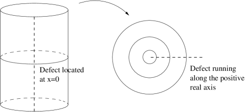
Figure 1: A defect placed at $x{=}0$ on the infinite cylinder is mapped to the positive real axis; states in the Hilbert space corresponds to fields located at the origin of the plane, that is fields living at.the end of the defect.

The identity defect, $(0,0)$, is invisible to all fields, in other words it is the formal solution of the defect equations (16) which corresponds to the absence of any defect whatsoever. This means that the Hilbert space containing the defect is the same as the Hilbert space in the absence of a defect -

$$\mathcal{H}^{(0,0)}=V_{0}\otimes\bar{V}_{0}+V_{1}\otimes\bar{V}_{1}\;,$$ (19)

and the corresponding highest weight states are ${|\,0,0\,\rangle}={|\,0\,\rangle}$ and ${|\,h,h\,\rangle}={|\,\Phi\,\rangle}$. Furthermore, the operators living on the defect are just the bulk fields with the same operator algebra.

In the case of the $(1,1)$ defect, the Hilbert space decomposes as [21]

$$\mathcal{H}^{d}=V_{1}\otimes\bar{V}_{0}+V_{0}\otimes\bar{V}_{1}+V_{1}\otimes\bar{V}_{1}$$ (20)

The corresponding highest weight states will be denoted as

$$|d\rangle=|h,0\rangle\quad;\qquad|\bar{d}\rangle=|0,h\rangle\quad;\qquad|D\rangle=|h,h\rangle$$ (21)

and they form (up to signs) an ortho-normal basis. These highest weight states correspond to fields which can be located at the end of the defect, or “create” the defect, as in figure 1. Similarly to the bulk normalization eq. (7) we choose the normalization $\langle D|D\rangle=-1$.

The operators living (not at the end but) on the defect correspond to the Hilbert space of the model on a circle where the defect runs along the whole real line, so that fields at the origin are located on the defect, as in figure 2. When mapped back to the cylinder, this corresponds to a cylinder with two defects [21]:

$$\mathcal{H}^{(1,1)}=V_{0}\otimes\bar{V}_{0}+V_{1}\otimes\bar{V}_{0}+V_{0}\otimes\bar{V}_{1}+2\,V_{1}\otimes\bar{V}_{1}$$ (22)

The h.w. vectors of these representation spaces we correspond to the following primary defect fields $\mathbb{I}$, $\varphi$, $\bar{\varphi}$, $\Phi_{-}$, $\Phi_{+}$, respectively. The non-chiral fields $\Phi_{\pm}$ can be taken to be the left/right limits of the bulk field $\Phi(z,\bar{z})$ on the defect. We calculate the structure constants of this defect conformal field theory in Appendix A by solving the sewing relations.

Figure 2: Two defects placed at $x{=}0$ and $x=\pi$ on the infinite cylinder are mapped to a single defect running along the whole real axis on the complex plane; states in the Hilbert space corresponds to fields located at the origin of the plane, that is fields living on the defect.

3 Massless perturbations

In this section we search for massless perturbations of the defect Lee-Yang model that preserve both energy and momentum. First we introduce a chiral holomorphic perturbation, then an anti-holomorphic one, finally we analyze a combination of chiral and anti-chiral perturbations.

Holomorphic perturbation

We consider a chiral holomorphic perturbation of the form

$$S=S_{DCFT}-\mu\int_{-\infty}^{\infty}dy\,\varphi(y)$$ (23)

As the action is dimensionless and the primary field has dimension $[\varphi]=h$ the dimension of the coupling constant is $[\mu]=1-h$. The perturbation on the defect does not affect the conservation laws in the bulk but it may change the bulk-defect OPE (18) or, consequently, the defect condition (16).

The change of the defect condition has a series expansion in $\mu$ which we can calculate in perturbation theory:

$$\Delta T(y):=T_{-}(y)-T_{+}(y)=\mu\mathcal{O}_{1}(y)+\mu^{2}\mathcal{O}_{2}(y)+\dots+\mu^{n}\mathcal{O}_{n}(y)+\dots$$ (24)

where $\mathcal{O}_{n}$ are operators localized on the defect. Each operator equation is understood within correlators in the perturbed theory, for renormalized operators. Comparing the dimensions of the two sides we observe that the dimension of the operator appearing, $\mathcal{O}_{n}$, has to be

$$[\mathcal{O}_{n}]=nh-n+2$$ (25)

As the most negative left chiral dimension is $-\frac{1}{5}$ the only non-vanishing contribution can appear for $n=1$ with $\mathcal{O}_{1}\propto\partial\varphi$.

As a consequence, the corresponding change in the bulk-defect OPE must have the form

$$T(x+iy)=\begin{cases}T^{R}(y)+b^{+}\,\mu\,\partial_{y}{\varphi}(y)+O(x)\;,&x>0\\ T^{R}(y)+b^{-}\,\mu\,\partial_{y}{\varphi}(y)+O(x)\;,&x<0\end{cases}\;,$$ (26)

where $T^{R}(y)$ is a suitably renormalised field and $b^{\pm}$ are constants.

However, the calculation of $b^{\pm}$ depends in detail on the regulation of divergences in the perturbation expansion and the precise definitions of the bulk and defect fields in the perturbed theory. We shall regulate the perturbation expansion using a hard cut-off $\epsilon$, so that in (23) the integration is only over values $y$ such that $|y-z|>\epsilon$ where $z$ is the insertion point of any other local field, either bulk or defect.

When the field $T(x+iy)$ approaches to within a distance $\epsilon$ of the defect, because the perturbation is cut off at distances less than $\epsilon$ the effect of the perturbation is reduced. As $x\to 0$, with $\epsilon$ fixed, the defect appears unperturbed and the structure constants $b^{\pm}$ go to zero. It is possible to keep careful track throughout our calculations of whether fields approach closer than $\epsilon$ to a defect, but to simplify the discussion we shall always assume that the limit $\epsilon\to 0$ is taken before any other limits. With this assumption, we find that $b^{\pm}=\mp i\pi(1-h)$ (see appendix B for details) and so

$$\Delta T(y) := \lim_{x\to 0^{+}}(T_{-}(-x+iy)-T_{+}(x+iy))$$ (27)

$$= \lim_{x\to 0^{+}}\lim_{\epsilon\to 0}(T_{-}(-x+iy)-T_{+}(x+iy))$$

$$= 2\pi i(1-h)\mu\,\partial_{y}\varphi(y)\;.$$

The anti-holomorphic part is not changed, $\Delta\bar{T}=0$.

This first order perturbative result is exact to any order in $\mu$:

$$\Delta T_{0}(y)e^{\mu\int_{-\infty}^{\infty}dy^{\prime}\,\varphi(y^{\prime})}=2\pi\mu(1-h)i(\partial_{y}\varphi(y))e^{\mu\int_{-\infty}^{\infty}dy^{\prime}\,\varphi(y^{\prime})}$$ (28)

where here and from now on operator products are always time ($y$) ordered, which we do not write out explicitly.

As the jump of the energy momentum tensor is a total derivative we can define the conserved energy as

$$H=H_{-}+H_{+}+2\pi\mu(1-h)\varphi$$ (29)

The existence of a conserved energy is not very surprising as our system is invariant under time translations. What is more surprising is that the momentum

$$P=P_{-}+P_{+}+2\pi\mu(1-h)\varphi$$ (30)

is also conserved, although we do not have translational invariance. This also means that the defect remains topological after the perturbation.

As there are only two topological defect conditions we expect a defect flow from the $\mathcal{H}^{d}$ defect to the $\mathcal{H}^{(0,0)}$ identity defect as the coupling constant ${\mu}$ increases. If we plot the eigenvalues of the dimensionless operator $\frac{HL}{2\pi}$, as a function of the dimensionless parameter $\mu L^{6/5}$ we can identify the states in both Hilbert spaces as well as the flows.

Lattice calculations [23] give a lot of information on these flows; in particular they describe the whole space of flows, in the following sense.

The UV endpoint of a flow is an energy and momentum eigenstate in the ${\cal H}^{d}$ space. This means it is an eigenstate of both $L_{0}$ and $\bar{L}_{0}$ and so is a descendant at $L_{0}$–level $M$ and $\bar{L}_{0}$–level $\bar{N}$ of some highest weight state in ${\cal H}^{d}$. Hence the UV endpoints of the flows form a distinguished basis of states and (from the results in section 2) we can label them by two sets of integers, $\{m_{i};\bar{n}_{j}\}$ satisfying $\sum_{i}m_{i}=M$ and $\sum_{j}\bar{n}_{j}=\bar{N}$ and certain other restrictions, depending on the sector in the Hilbert space.

Likewise, the IR endpoints of the flows determine a distinguished basis of states in ${\cal H}^{(0,0)}$ labelled by another two sets of integers $\{m^{\prime}_{i};\bar{n}^{\prime}_{j}\}$ satisfying another set of restrictions. Since the flow is entirely holomorphic, the anti-holomorphic representation cannot change and $\bar{n}^{\prime}_{j}=\bar{n}_{j}$ but the lattice calculations in [23] indicate that the holomorphic representations and the integers $\{m^{\prime}_{i}\}$ and $\{m_{i}\}$ are related as in table 1.

$$\begin{array}[]{c|rcl|c}\hbox{UV}&&&&\hbox{IR}\\ \hline\cr(d)&\{m_{1},\cdots,m_{l};{\bar{n}}_{1},\cdots,{\bar{n}}_{k}\}&\longrightarrow&\{m_{1}{+}1,\cdots,m_{l}{+}1;{\bar{n}}_{1},\cdots,{\bar{n}}_{k}\}&(0,0)\\ &\lx@intercol\hfil m_{l}\geq 1\;,\;\;{\bar{n}}_{k}\geq 2\hfil\lx@intercol\vrule\lx@intercol\\ \hline\cr(\bar{d})&\{m_{1},\cdots,m_{l};{\bar{n}}_{1},\cdots,{\bar{n}}_{k}\}&\longrightarrow&\{m_{1}{+}1,\cdots,m_{l}{+}1,1;{\bar{n}}_{1},\cdots,{\bar{n}}_{k}\}&(h,h)\\ &\lx@intercol\hfil m_{l}\geq 2\;,\;\;{\bar{n}}_{k}\geq 1\hfil\lx@intercol\vrule\lx@intercol\\ \hline\cr(D)&\{m_{1},\cdots,m_{l};{\bar{n}}_{1},\cdots,{\bar{n}}_{k}\}&\longrightarrow&\{m_{1}{+}1,\cdots,m_{l}{+}1;{\bar{n}}_{1},\cdots,{\bar{n}}_{k}\}&(h,h)\\ &\lx@intercol\hfil m_{l}\geq 1\;,\;\;\bar{n}_{k}\geq 1\hfil\lx@intercol\vrule\lx@intercol\\ \hline\cr\end{array}$$

Table 1: The UV and IR endpoints of the defect flows for a purely holomorphic perturbation. In each case $\{m_{i}\}$ and $\{\bar{n}_{j}\}$ satisfy $m_{l}\geq m_{l{+}1}+2$ and ${\bar{n}}_{k}\geq{\bar{n}}_{k{+}1}+2$.

When the energy eigenspaces in question are one-dimensional then the flows are uniquely defined, as is the case for the flows starting from the 24 lowest-lying states in ${\cal H}^{d}$. Their flows are given in table 2.

Energy	$\mathcal{H}^{d}$	$\mathcal{H}^{\left(0,0\right)}$	Energy
$-\frac{2}{5}$	$|D\rangle$	$|h,h\rangle$	$-\frac{2}{5}$
$-\frac{1}{5}$	$|\bar{d}\rangle$	$|0,0\rangle$	$0$
	$|d\rangle$	$\bar{L}_{-1}|h,h\rangle$	$\frac{3}{5}$
$\frac{3}{5}$	$L_{-1}|D\rangle$	$L_{-1}|h,h\rangle$
	$\bar{L}_{-1}|D\rangle$	$\bar{L}_{-2}|h,h\rangle$	$\frac{8}{5}$
$\frac{4}{5}$	$L_{-1}|d\rangle$	$L_{-1}\bar{L}_{-1}|h,h\rangle$
	$\bar{L}_{-1}|\bar{d}\rangle$	$\bar{L}_{-2}|0,0\rangle$	$2$
$\frac{8}{5}$	$L_{-2}|D\rangle$	$L_{-2}|h,h\rangle$	$\frac{8}{5}$
	$\bar{L}_{-2}|D\rangle$	$\bar{L}_{-3}|h,h\rangle$	$\frac{13}{5}$
	$L_{-1}\bar{L}_{-1}|D\rangle$	$L_{-1}\bar{L}_{-2}|h,h\rangle$
$\frac{9}{5}$	$L_{-2}|\bar{d}\rangle$	$L_{-2}|0,0\rangle$	$2$
	$L_{-2}|d\rangle$	$L_{-2}\bar{L}_{-1}|h,h\rangle$	$\frac{13}{5}$
	$\bar{L}_{2}|\bar{d}\rangle$	$\bar{L}_{-3}|0,0\rangle$	$3$
	$\bar{L}_{-2}|d\rangle$	$\bar{L}_{-3}\bar{L}_{-1}|h,h\rangle$	$\frac{18}{5}$
$\frac{13}{5}$	$L_{-3}|D\rangle$	$L_{-3}|h,h\rangle$	$\frac{13}{5}$
	$\bar{L}_{-3}|D\rangle$	$\bar{L}_{-4}|h,h\rangle$	$\frac{18}{5}$
	$L_{-2}\bar{L}_{-1}|D\rangle$	$L_{-2}\bar{L}_{-2}|h,h\rangle$
	$L_{-1}\bar{L}_{-2}|D\rangle$	$L_{-1}\bar{L}_{-3}|h,h\rangle$
$\frac{14}{5}$	$L_{-3}|\bar{d}\rangle$	$L_{-3}|0,0\rangle$	$3$
	$L_{-3}|d\rangle$	$L_{-3}\bar{L}_{-1}|h,h\rangle$	$\frac{18}{5}$
	$L_{-2}\bar{L}_{-1}|\bar{d}\rangle$	$L_{-2}\bar{L}_{-2}|0,0\rangle$	$4$
	$\bar{L}_{-3}|\bar{d}\rangle$	$\bar{L}_{-4}|0,0\rangle$
	$\bar{L}_{-3}|d\rangle$	$\bar{L}_{-4}\bar{L}_{-1}|h,h\rangle$	$\frac{23}{5}$
	$L_{-1}\bar{L}_{-2}|d\rangle$	$L_{-1}\bar{L}_{-3}\bar{L}_{-1}|h,h\rangle$

Table 2: Defect flows in the case of a purely holomorphic perturbation. The flows starting from the lowest-lying 24 states in ${\cal H}^{d}$ are uniquely determined by the lattice calculations in [23] given in Table 1.

We can identify these flows if we plot the eigenvalues of ${HL}/({2\pi})$ against $\log(L\mu^{5/6})$, as we do in figure 3.

Figure 3: Defect flows in the case of a purely holomorphic perturbation calculated from DTCSA; the subtracted energies $[(E_{i}-E_{0})L/(2\pi)-2/5]$ are plotted against $\log(\mu L^{5/6})$. The flows go from the spectrum of the UV defect ${\cal H}^{d}$ on the left to the IR defect ${\cal H}^{(0,0)}$ on the right. The degeneracies of the states are shown in brackets.

Anti-holomorphic perturbation

Let us introduce a purely anti-holomorphic perturbation of the form

$$S=S_{DCFT}-\bar{\mu}\int_{-\infty}^{\infty}dy\,\bar{\varphi}(y)\;,$$ (31)

and see how the formulae above change. Clearly only the anti-holomorphic part is affected now ($\Delta T=0$). An analogous argument and calculation gives the exact result for the change of the defect condition:

$$\Delta\bar{T}(y)=-2\pi\bar{\mu}(1-h)i\partial_{y}\bar{\varphi}(y)\;.$$ (32)

This leads to the conserved energy and momentum in the form

$$H=H_{-}+H_{+}+2\pi\bar{\mu}(1-h)\bar{\varphi}\quad;\qquad P=P_{-}+P_{+}-2\pi\bar{\mu}(1-h)\bar{\varphi}\;.$$ (33)

The anti-holomorphic defect flow can be obtained from the holomorphic one by a trivial (left-right) replacement.

Combined holomorphic and anti-holomorphic perturbations

We can try to combine holomorphic and anti-holomorphic perturbations of the form

$$S=S_{DCFT}-\int_{-\infty}^{\infty}\left(\mu\varphi(y)+\bar{\mu}\bar{\varphi}(y)\right)dy$$ (34)

The jump of the chiral half of the energy momentum tensor is given by

$$\Delta T(y)=\lim_{x\to 0}\lim_{\epsilon\to 0}\left((T_{0}(-x+iy)-T_{0}(x+iy))e^{\int_{-\infty}^{\infty}\left(\bar{\mu}\bar{\varphi}(y^{\prime})+\mu\varphi(y^{\prime})\right)dy^{\prime}}\right)$$ (35)

which has an expansion of the form

$$\Delta T=\mu\mathcal{O}_{1}+\bar{\mu}\mathcal{O}_{\bar{1}}+\mu^{2}\mathcal{O}_{2}+\bar{\mu}^{2}\mathcal{O}_{\bar{2}}+\mu\bar{\mu}\mathcal{O}_{1\bar{1}}+\dots$$ (36)

Comparing the dimensions we can write

$$[\mathcal{O}_{n\bar{n}}]=(n+\bar{n})h-n-\bar{n}+2$$ (37)

clearly we have the previous solutions for $n=1$, $\bar{n}=0$ with $\mathcal{O}_{1}\propto\partial\varphi$. (Alternatively, for $\Delta\bar{T}$ we have $n=0$, $\bar{n}=1$ with $\mathcal{O}_{\bar{1}}\propto\bar{\partial}\bar{\varphi}$). Additionally, to these cases we also have the possibility $n=\bar{n}=1$ with either of the two equivalent expressions,

$$\mathcal{O}_{1\bar{1}}(y) = d_{+}\varphi(y)\bar{\varphi}(y)+d_{-}\bar{\varphi}(y)\varphi(y)$$ (38)

$$= c_{+}\Phi_{+}(y)+c_{-}\Phi_{-}(y)$$ (39)

In Appendix B we calculate $d_{\pm},c_{\pm}$ by carefully taking into account the contribution of $\mathcal{O}_{1}$ to $\Delta T$ at order $\mu\bar{\mu}$. As a result we obtain

$$d_{\pm}=\pm 2\pi i\,h\;,$$ (40)

and equivalently

$$c_{\pm}=2\pi ihC_{[\varphi,\bar{\varphi}]}^{\pm}\qquad;\qquad C_{[\varphi,\bar{\varphi}]}^{\pm}=C_{\varphi\bar{\varphi}}^{\pm}-C_{\bar{\varphi}\varphi}^{\pm}$$ (41)

Summarising, this means that

$$\frac{\Delta T}{2\pi i}=(1-h)\mu\partial_{y}\varphi\;+\;\mu\bar{\mu}hC_{[\varphi,\bar{\varphi}]}^{+}\Delta\Phi$$ (42)

where $\Delta\Phi=\lim_{x\to+0}(\Phi(-x+iy)-\Phi(x+iy))=\Phi_{-}-\Phi_{+}$.

Some caution is required here: First note that holomorphic and anti-holomorphic defect fields do not necessarily commute. By conformal invariance their OPE should start with a regular term and if they were bulk fields this would imply that moving one field around the other no monodromy is picked up thus they would commute. Defect fields, however live only on the defects and we do not have the possibility to exchange the two fields without leaving the defect. Since the perturbation includes the non-commuting anti-chiral and chiral fields $\bar{\varphi}$, $\varphi$, the time derivative $\partial_{y}\varphi(y)$ taken in the unperturbed theory is not the same as the total time derivative of the field calculated in the perturbed theory. Instead we have

$$[\partial_{y}\varphi]_{tot}:=\partial_{y}(e^{-\delta S}\varphi)=e^{-\delta S}\left(\partial_{y}\varphi+\bar{\mu}[\varphi,\bar{\varphi}]\right)\;.$$ (43)

Since it is the total time-derivative we are interested in, we have the final result for the jump in $T$,

$$\frac{\Delta T}{2\pi i}=(1-h)\left[\mu\partial_{y}\varphi\right]_{tot}\;+\;\mu\bar{\mu}\,C_{[\varphi,\bar{\varphi}]}^{+}\Delta\Phi\;.$$ (44)

This can be a total time derivative only for chiral perturbations, i.e. when either $\mu$ or $\bar{\mu}$ vanishes. Similarly we obtain

$$\frac{\Delta\bar{T}}{2\pi i}=-(1-h)\left[\bar{\mu}\partial_{y}\bar{\varphi}\right]_{tot}\;+\;\mu\bar{\mu}\,C_{[\varphi,\bar{\varphi}]}^{+}\Delta\Phi$$ (45)

Clearly in calculating the energy, the jump $\Delta T-\Delta\bar{T}$ is a total $y$–derivative and so a conserved energy can be defined, as we expected from time-translation invariance. This is not true for the momentum, where $\Delta T+\Delta\bar{T}$ is not a total $y$–derivative. The special form of the non-derivative term which does appear however, ($\Delta\Phi$), enables us to cancel it by introducing an appropriately chosen bulk perturbation.

4 Massive perturbations

We start by analyzing a purely bulk perturbation without any defect.

Pure bulk perturbation

The perturbed action is given by

$$S=S_{0}-\lambda\int dudv\,\Phi(u,v)=S_{0}-\lambda\int d^{2}w\,\Phi(w,\bar{w})$$ (46)

The corresponding change in the conservation law comes from $\bar{\partial}T\neq 0$ and can be calculated in a perturbative expansion

$$\partial_{\bar{z}}T(z)=\partial_{\bar{z}}\left(T_{0}(z)e^{\lambda\int d^{2}w\,\Phi(w,\bar{w})}\right)=\lambda\mathcal{O}_{1}+\lambda^{2}\mathcal{O}_{2}+\dots$$ (47)

Dimensional argumentation shows that the only perturbative contribution comes from the first order term:

$$\partial_{\bar{z}}\left(T_{0}(z)\Phi(w,\bar{w})\right)=\partial_{\bar{z}}\left(\frac{h\Phi(w,\bar{w})}{(z-w)^{2}}+\frac{\partial_{w}\Phi(w,\bar{w})}{(z-w)}\right)$$ (48)

We use that

$$\partial_{\bar{z}}\frac{1}{z-w}=\pi\delta^{(2)}(z-w)\qquad;\qquad\partial_{\bar{z}}\frac{1}{(z-w)^{2}}=\pi\partial_{w}\delta^{(2)}(z-w)$$ (49)

and integrate by parts. Assuming fields vanish at infinities we can drop the surface term and obtain:

$$\partial_{\bar{z}}T(z)=\pi\lambda(1-h)\partial_{z}\Phi(z,\bar{z})\equiv\partial_{z}\Theta(z,\bar{z})$$ (50)

From the dimensional argument we conclude that there are no higher order terms. We have a similar expression for the anti-holomorphic part

$$\partial_{z}\bar{T}(\bar{z})=\pi\lambda(1-h)\partial_{\bar{z}}\Phi(z,\bar{z})\equiv\partial_{\bar{z}}\bar{\Theta}(z,\bar{z})$$ (51)

These conserved currents lead to conserved charges:

$$H=\int_{-\infty}^{\infty}dx\,(T(z)+\bar{T}(\bar{z})+2\pi\lambda(1-h)\Phi(z,\bar{z}))\;;\quad P=\int_{-\infty}^{\infty}dx\,(T(z)-\bar{T}(\bar{z}))$$ (52)

and so their conservation follows as we have to integrate a total derivative:

$$\dot{H}=i\int_{-\infty}^{\infty}dx\,\partial_{x}(T(z)-\bar{T}(\bar{z}))\;;\quad\dot{P}=i\int_{-\infty}^{\infty}dx\,\partial_{x}(T(z)+\bar{T}(\bar{z})-2\pi\lambda(1-h)\Phi(z,\bar{z}))$$ (53)

If we introduce the defect, then the local conservation laws are not changed but we have to be careful with the surface terms at the defect. As before, we will cut off all perturbative integrals at a distance $\epsilon$ and we will take $\epsilon\to 0$ before any other limits.

Using this convention, we find in appendix B that the bulk perturbation introduces jumps in the energy momentum tensor of the form

$$\Delta T(y)=-\lambda\pi h\,\Delta\Phi(y)\;,\;\;\Delta\bar{T}(y)=-\lambda\pi h\,\Delta\Phi(y)$$ (54)

Defining $H_{\pm}$ and $P_{\pm}$ by splitting the integrals in eq. (52) as we did in eq. (12,14):

$$H=H_{-}+H_{+}\quad;\qquad P=P_{-}+P_{+}$$ (55)

we can easily see that

$$\partial_{y}H=i\left[\Delta T-\Delta\bar{T}\right]=0\;,\;\;\;\;\partial_{y}P=i\left[\Delta T+\Delta\bar{T}-2\pi\lambda(1-h)\Delta\Phi\right]=-2\pi i\,\lambda\,\Delta\Phi\neq 0$$ (56)

Clearly the defect perturbation, without any defect field is not integrable. As the form of $\partial_{y}P$ is the same as the contribution of the combined holomorphic and anti-holomorphic defect perturbation: eq. (44,45) by properly synchronizing their coefficients we can ensure integrability.

Combined bulk and defect perturbation

Now we introduce simultaneously the bulk perturbation and the chiral and anti-chiral defect perturbations:

$$S=S_{DCFT}-\lambda\int d^{2}w\,\Phi(w,\bar{w})-\int_{-\infty}^{\infty}\left(\mu\varphi(y)+\bar{\mu}\bar{\varphi}(y)\right)dy$$ (57)

From appendix B we see that the jumps in $T$ and $\bar{T}$ in the case of the combined perturbation are

$$\Delta T(y) = 2\pi i(1-h)\mu[\partial_{y}\varphi]_{tot}+(2\pi i\mu\bar{\mu}C^{+}_{[\varphi,\bar{\varphi}]}-\lambda\pi h)\Delta\Phi\;,$$ (58)

$$\Delta\bar{T}(y) = -2\pi i(1-h)\bar{\mu}[\partial_{y}\bar{\varphi}]_{tot}+(2\pi i\mu\bar{\mu}C^{+}_{[\varphi,\bar{\varphi}]}-\lambda\pi h)\Delta\Phi\;.$$ (59)

Using the bulk conservation laws, we find

$$\partial_{y}(H_{-}+H_{+}) = i(\Delta T-\Delta\bar{T})$$ (60)

$$= -2\pi(1-h)[\partial_{y}(\mu\varphi+\bar{\mu}\bar{\varphi})]_{tot}\;,$$

is always a total $y$–derivative and hence the total energy $H$ defined as

$$H=H_{-}+H_{+}+2\pi(1-h)(\mu\varphi+\bar{\mu}\bar{\varphi})\;,$$ (61)

is always conserved.

We also find

$$\partial_{y}(P_{-}+P_{+}) = i(\Delta T+\Delta\bar{T}-2\pi\lambda(1-h)\Delta\Phi)$$ (62)

$$= -2\pi(1-h)[\partial_{y}(\mu\varphi-\bar{\mu}\bar{\varphi})]_{tot}-(4\pi\mu\bar{\mu}C^{+}_{[\varphi,\bar{\varphi}]}+2i\lambda\pi)\Delta\Phi$$

is a total derivative if $\lambda=2i\mu\bar{\mu}C^{+}_{[\varphi,\bar{\varphi}]}$. Hence, we can define a total momentum

$$P=P_{-}+P_{+}+2\pi(1-h)(\mu\varphi-\bar{\mu}\bar{\varphi})\;,$$ (63)

which is conserved exactly when

$$\lambda=2i\mu\bar{\mu}C^{+}_{[\varphi,\bar{\varphi}]}=(0.826608\ldots)\,\mu\,\bar{\mu}\;.$$ (64)

This agrees with the result in [22] where the problem was analysed in the opposite channel. We can conclude that the perturbation is integrable only if this constraint is satisfied. As $\lambda$ defines the mass scale, the space of integrable defect perturbations has one physical parameter. Observe also that we cannot switch off the defect perturbations completely if we insist on keeping integrability.

5 Defect TCSA

In this section we review the TCSA method for periodic boundary conditions and generalize it for the defect case.

The theory is defined on the cylinder of circumference $L$. The periodic Hilbert space takes the form

$$\mathcal{H}=V_{0}\otimes\bar{V}_{0}+V_{1}\otimes\bar{V}_{1}$$ (65)

where the unperturbed Hamiltonian acts as

$$H_{0}=\frac{2\pi}{L}\left(L_{0}+\bar{L}_{0}-\frac{c}{12}\right)$$ (66)

The perturbation which defines the scaling Lee-Yang model on the cylinder is given by

$$H=H_{0}-\lambda\int_{0}^{L}\Phi(x,0)dx\;.$$ (67)

Mapping the cylinder onto the plane, ($\zeta=x+iy\to z=e^{-i\frac{2\pi}{L}\zeta}=re^{i\theta}$, $\bar{z}=e^{i\frac{2\pi}{L}\bar{\zeta}}=re^{-i\theta}$), we find the Hamiltonian is given by

$$H=\frac{2\pi}{L}\left[\;L_{0}+\bar{L}_{0}+\frac{11}{30}+\lambda\left(\frac{L}{2\pi}\right)^{2+\frac{2}{5}}\!\int_{0}^{-2\pi}\!\!\!d\theta\,\Phi(e^{i\theta},e^{-i\theta})\;\right]\;.$$ (68)

The rotation operator on the plane $L_{0}-\bar{L}_{0}$ corresponds to the momentum operator on the cylinder $P=\frac{2\pi}{L}(L_{0}-\bar{L}_{0})$. As a result the $\theta$-dependence of the matrix elements of the perturbing operator can be easily evaluated and the integral gives momentum conservation:

$$\int_{0}^{-2\pi}\langle j|\Phi(e^{i\theta},e^{-i\theta}){|\,k\,\rangle}d\theta=\int_{0}^{-2\pi}e^{i\theta(h_{k}-\bar{h}_{k}-h_{j}+\bar{h}_{j})}d\theta\,\Phi_{jk}=-\Phi_{jk}2\pi\delta_{P_{k}-P_{j}}$$ (69)

where $\Phi_{jk}=\langle j|\Phi(1,1)|k\rangle$ and we used that $h_{k}-\bar{h}_{k}\in\mathbb{Z}$. Introducing the inner product matrix $G_{ij}=\langle i|j\rangle$ and the mass gap relation (89) the dimensionless Hamiltonian can be written as

$$\frac{H}{m}=\frac{2\pi}{mL}\left[\;L_{0}+\bar{L}_{0}+\frac{11}{30}-\left(\frac{mL}{2\pi\kappa}\right)^{\frac{12}{5}}(2\pi)\,G^{-1}\Phi\;\right]$$ (70)

Pure defect perturbation

The defect conformal Hilbert space contains the modules

$$\mathcal{H}^{d}=V_{1}\otimes\bar{V}_{0}+V_{0}\otimes\bar{V}_{1}+V_{1}\otimes\bar{V}_{1}$$ (71)

and the unperturbed Hamiltonian is given by eq. (66).

We start by analyzing a chiral defect perturbation of the form

$$H=H_{0}-\mu\varphi(y=0)$$ (72)

We map the cylinder to the conformal plane ($\zeta=x+iy\to z=e^{-i\frac{2\pi}{L}\zeta}$, such that the defect $x=0$ will fill the real positive line: $z=e^{\frac{2\pi}{L}y}$). As the defect field is chiral it will acquire an additional phase, $\rho=e^{i\pi/10}$. To distinguish between the cases when the defect is located on the imaginary $\varphi(iy)$ or on the real $\varphi(x)$ line we introduce another coupling $\hat{\mu}=\mu\rho$, such that

$$\mu\varphi(ix)=\hat{\mu}\varphi(x)\qquad;\quad\hat{\mu}=\mu\rho\quad;\quad\rho=e^{i\frac{\pi}{10}}$$ (73)

With this coupling the Hamiltonian on the plane is

$$H=\frac{2\pi}{L}\left[L_{0}+\bar{L}_{0}-\frac{c}{12}-\hat{\mu}\left(\frac{L}{2\pi}\right)^{1+\frac{1}{5}}\varphi(1)\right]$$ (74)

For numerical evaluation we will need the various matrix elements of $\varphi$, which are evaluated in Appendix A:

$$C_{\varphi D}^{D}=C_{\varphi\varphi}^{\varphi}=\alpha\beta^{-1}\quad;\quad C_{\varphi d}^{d}=\,\alpha\beta\quad;\quad C_{\varphi D}^{\bar{d}}=-C_{\varphi\bar{d}}^{D}=1$$ (75)

where

$$\alpha=\sqrt{\frac{\Gamma(\frac{1}{5})\Gamma(\frac{6}{5})}{\Gamma(\frac{3}{5})\Gamma(\frac{4}{5})}}\quad;\qquad\beta=\sqrt{\frac{2}{1+\sqrt{5}}}$$ (76)

Combined bulk and defect perturbation

Now we perturb the conformal defect theory simultaneously in the bulk and at the defect

$$H=H_{0}-\lambda\int_{0}^{L}\Phi(x,0)dx-\mu\varphi(0)-\bar{\mu}\bar{\varphi}(0)$$ (77)

Mapping the system onto the plane

$$H=\frac{2\pi}{L}\left[\;L_{0}+\bar{L}_{0}+\frac{11}{30}-\left(\frac{L}{2\pi}\right)^{\!1+\frac{1}{5}}\left(\hat{\mu}\varphi(1)+\hat{\bar{\mu}}\bar{\varphi}(1)\right)+\lambda\left(\frac{L}{2\pi}\right)^{\!2+\frac{2}{5}}\!\int_{0}^{-2\pi}d\theta\,\Phi(e^{i\theta},e^{-i\theta})\;\right]$$ (78)

where $\hat{\bar{\mu}}=\bar{\mu}\rho^{-1}$. Using the rotation symmetry we can perform the integrals

$$\rho_{jk}:=\int_{0}^{-2\pi}e^{i\theta S_{jk}}d\theta=\begin{cases}\begin{array}[]{c}-2\pi\\ -2e^{-i\pi S_{jk}}\frac{\sin\pi S_{jk}}{S_{jk}}\end{array}&\begin{array}[]{c}\mbox{ if }S_{jk}=0\\ \mbox{otherwise}\end{array}\end{cases}$$ (79)

where the difference of the spins

$$S_{jk}:=h_{j}-\bar{h}_{j}-h_{k}+\bar{h}_{k}$$ (80)

is usually not an integer. The matrix form of the dimensionless Hamiltonian is simply

$$\frac{H}{m}=\frac{2\pi}{mL}\left[L_{0}+\bar{L}_{0}+\frac{11}{30}-\left(\frac{L}{2\pi}\right)^{\frac{6}{5}}G^{-1}\left(\hat{\mu}\varphi+\hat{\bar{\mu}}\bar{\varphi}\right)+\left(\frac{mL}{2\pi\kappa}\right)^{\frac{12}{5}}\,G^{-1}\,\Phi_{\rho}\right]$$ (81)

where $\langle j|\Phi_{\rho}{|\,k\,\rangle}=\Phi_{jk}\rho_{jk}$.

The relevant structure constants are

$$C_{\varphi\bar{\varphi}}^{\Phi_{-}}=C_{\bar{\varphi}\varphi}^{\Phi_{+}}=\frac{\beta^{-1}}{1+\eta^{-1}}\qquad;\qquad C_{\varphi\bar{\varphi}}^{\Phi_{+}}=C_{\bar{\varphi}\varphi}^{\Phi_{-}}=\frac{\beta^{-1}}{1+\eta}$$ (82)

$$C_{\Phi_{-}d}^{\bar{d}}=-\eta^{-2}\beta^{-1}\quad;\quad C_{\Phi_{-}\bar{d}}^{d}=-\eta^{2}\beta^{-1}\quad;\quad C_{\Phi_{-}d}^{D}=-\eta^{-1}\alpha\quad;\quad C_{\Phi_{-}D}^{\bar{d}}=\eta^{-1}\alpha$$ (83)

$$C_{\Phi_{-}\bar{d}}^{D}=-\eta\alpha\quad;\quad C_{\Phi_{-}D}^{d}=\eta\alpha\quad;\quad C_{\Phi_{-}D}^{D}=\alpha^{2}\beta^{-1}$$ (84)

Integrability in DTCSA

It is interesting to analyze the integrability of the model by demanding the commutation of energy and momentum $[H,P]=0.$ The momentum in the TCSA scheme is given by

$$P=\frac{2\pi}{L}\left[L_{0}-\overline{L}_{0}-\left(\frac{L}{2\pi}\right)^{\frac{6}{5}}\hat{\mu}\varphi(1)+\left(\frac{L}{2\pi}\right)^{\frac{6}{5}}\hat{\bar{\mu}}\bar{\varphi}(1)\right]$$ (85)

while the energy by (78). We perform the analysis for $L=2\pi$.

The term $\left[L_{0}+\overline{L}_{0},\ \hat{\mu}\varphi(1)-\hat{\bar{\mu}}\bar{\varphi}(1)\right]$ cancels against $\left[\hat{\mu}\varphi(1)+\hat{\bar{\mu}}\bar{\varphi}(1),\ L_{0}-\overline{L}_{0}\right].$ Using the identity $\left[L_{0},\ \Phi\left(z,\bar{z}\right)\right]=h\Phi(z,\bar{z})+z\partial_{z}\Phi(z,\bar{z})$, its anti-holomorphic part together with $z\partial_{z}-\bar{z}\partial_{\bar{z}}=-i\partial_{\theta,}$ we can write

$$\lambda\int_{0}^{-2\pi}\left[\Phi\left(e^{i\theta},e^{-i\theta}\right),\ L_{0}-\overline{L}_{0}\right]d\theta = \lambda i\int_{0}^{-2\pi}\partial_{\theta}\Phi(e^{i\theta},e^{-i\theta})d\theta$$ (86)

$$= -i\lambda\left(\Phi_{+}(1)-\Phi_{-}(1)\right)\;.$$

This term has to cancel against $2\hat{\mu}\hat{\bar{\mu}}\left[\bar{\varphi}(1),\ \varphi(1)\right]=-2\hat{\mu}\hat{\bar{\mu}}C^{+}_{[\varphi,\bar{\varphi}]}(\Phi_{+}-\Phi_{-})$ which leads to

$$\hat{\mu}\hat{\bar{\mu}}=\mu\bar{\mu}=\lambda\frac{1}{2iC^{+}_{[\varphi,\bar{\varphi}]}}\;,\;\;\;\;C^{+}_{[\varphi,\bar{\varphi}]}=C_{\varphi\bar{\varphi}}^{\Phi_{+}}-C_{\bar{\varphi}\varphi}^{\Phi_{+}}=\beta^{-1}\frac{1-\eta}{1+\eta}=-i\,0.413304\ldots$$ (87)

This result is the same as we calculated before.

Finally we analyze the term

$$\int_{0}^{-2\pi}\left[\Phi\left(e^{i\theta},e^{-i\theta}\right),\ \hat{\mu}\varphi(1)-\hat{\bar{\mu}}\bar{\varphi}(1)\right]d\theta.$$ (88)

Let’s denote $\psi(x)=\hat{\mu}\varphi(x)-\hat{\bar{\mu}}\bar{\varphi}(x)$. In taking the products of operators, they have to be radially ordered, therefore in the commutator the contour of the integration is deformed by $\epsilon$: in the $\Phi\psi$ term the radius of the integration is $1+\epsilon$, while in the $\psi\Phi$ term the radius is $1-\epsilon$. Then, the contour of the integration can be transformed: one integral from $1+\epsilon$ to $1-\epsilon$ on the upper side of the defect plus one integral from $1-\epsilon$ to $1+\epsilon$ on the lower side of the defect. The limit of $\Phi$ on the defect from above is $\Phi_{-}$, and the limit from below is $\Phi_{+}$. We can use the OPEs to calculate these integrals. The OPEs of $\Phi_{+}$ and $\Phi_{-}$ with $\varphi$ and $\bar{\varphi}$ are regular in $\epsilon$, and we can perform the integration. After the integration we get only positive power terms in $\epsilon$ which are vanishing in the $\epsilon\rightarrow 0$ limit, and so (88) is zero.

6 Scattering description of defects in the scaling Lee-Yang model

We summarise here the results of [10] on the integrable description of defects in the Lee-Yang model and give the UV-IR correspondence relating the parameters in the integrable and perturbed DCFT descriptions.

The scaling Lee-Yang model has a single massive particle with mass

$$m=\kappa\,\lambda^{\frac{5}{12}}\;,\;\;\;\;\kappa=\frac{2^{19/12}\sqrt{\pi}}{5^{5/16}}\,\frac{(\Gamma(3/5)\Gamma(4/5))^{5/12}}{\Gamma(2/3)\Gamma(5/6)}\,=2.642944\ldots\;,$$ (89)

and two-particle $S$–matrix

$$S(\theta)=-\left(\frac{1}{3}\right)\left(\frac{2}{3}\right)\;,\;\;\;\;(x)=\frac{\sinh(\frac{\theta}{2}+\frac{i\pi x}{2})}{\sinh(\frac{\theta}{2}-\frac{i\pi x}{2})}\;.$$ (90)

An integrable defect is described by two transmission factors, $T_{-}(\theta)$ for a particle crossing from left to right with rapidity $\theta>0$ and $T_{+}(-\theta)$ for a particle crossing from right to left with rapidity $\theta<0$. The authors of [10] proposed the following one-parameter family of solutions to the fusion, crossing and unitarity relations:

$$T_{-}=\left[b+1\right]\left[b-1\right]=S\Bigl{(}\theta-\frac{i\pi(3{-}b)}{6}\Bigr{)}\;,\;\;T_{+}=\left[5-b\right]\left[-5-b\right]=S\Bigl{(}\theta+\frac{i\pi(3{-}b)}{6}\Bigr{)}\;,\;\;$$ (91)

where

$$\left[x\right]=i\frac{\sinh\left(\frac{\theta}{2}+i\frac{\pi x}{12}\right)}{\sinh\left(\frac{\theta}{2}+i\frac{\pi x}{12}-i\frac{\pi}{2}\right)}\;.$$ (92)

Thus it can be seen that the defect is equivalent, for scattering purposes, to a particle with rapidity $i\pi(3-b)/6$, and the transmission factor is a pure phase for $b=\mp 3+i\alpha$.

According to [10] the bulk energy-density and the infinite volume defect energy are

$$\epsilon_{bulk}=-\frac{1}{4\sqrt{3}}m^{2}\qquad;\quad\epsilon_{Def}=m\sin\left(\frac{b\pi}{6}\right)\;,$$ (93)

and the finite size corrections for the ground state energy are also given, in first order, by the Lüscher correction term which is

$$E_{0}\left(L\right)=-m\int_{-\infty}^{\infty}\frac{d\theta}{2\pi}\cosh\left(\theta\right)T_{+}\left(\frac{i\pi}{2}-\theta\right)e^{-mL\cosh\left(\theta\right)}+O\left(e^{-2mL}\right)\;.$$ (94)

The Defect Thermodynamic Bethe Ansatz (DTBA) equations were also derived. The pseudo energy is given as the solution of the integral equation

$$\varepsilon\left(\theta\right)=mL\cosh\theta-\int_{-\infty}^{\infty}\frac{d\theta^{\prime}}{2\pi}\phi\left(\theta-\theta^{\prime}\right)\log\left(1+T_{+}\left(\frac{i\pi}{2}-\theta^{\prime}\right)e^{-\varepsilon\left(\theta^{\prime}\right)}\right)$$ (95)

where $\phi(\theta)=-i\frac{d}{d\theta}\log S(\theta)$. The ground state energy is expressed via the pseudo energy as

$$E_{0}\left(L\right)=-m\int_{-\infty}^{\infty}\frac{d\theta}{2\pi}\cosh\left(\theta\right)\log\left(1+T_{+}\left(\frac{i\pi}{2}-\theta\right)e^{-\varepsilon\left(\theta\right)}\right)$$ (96)

The DTBA equations are reliable at least for such values of the defect parameter $b$ when the transmission factor $T_{+}$ is a pure phase, i. e. for $b=-3+i\alpha$ with real $\alpha$.

There are several ways to derive the UV-IR correspondence. One is by comparing the action of the defect on the identity boundary condition with the perturbed boundary condition $\Phi(b)$. As the defect approaches the boundary, the two defect fields $\varphi(x)$ and $\bar{\varphi}(x)$ both have the same limit, the relevant boundary field $\phi(x)$, so that the defect perturbation with parameters $(\hat{\mu},\hat{\bar{\mu}})$ becomes the boundary perturbation with parameter $h=\hat{\mu}+\hat{\bar{\mu}}$, $\hat{\mu}\varphi+\hat{\bar{\mu}}\bar{\varphi}\to(\hat{\mu}+\hat{\bar{\mu}})\phi$. The boundary UV-IR relation is [24]:

$$h=|h_{c}|\cos((b+3)\pi/5)m^{6/5}=\frac{|h_{c}|m^{6/5}}{2}\,e^{(b+3)\pi i/5}\;+\;\frac{|h_{c}|m^{6/5}}{2}\,e^{-(b+3)\pi i/5}\;,\;\;\;\;$$ (97)

$$h_{c}=-\frac{\pi^{3/5}2^{4/5}5^{1/4}\sin\frac{2\pi}{5}}{(\Gamma(\frac{3}{5})\Gamma(\frac{4}{5}))^{1/2}}\left(\frac{\Gamma(\frac{2}{3})}{\Gamma(\frac{1}{6})}\right)^{6/5}=-0.685289\ldots\;.$$ (98)

The natural identification is

$$\hat{\mu}=\frac{|h_{c}|m^{6/5}}{2}\,e^{\pm i(b+3)\pi/5}\;,\;\;\hat{\bar{\mu}}=\frac{|h_{c}|m^{6/5}}{2}\,e^{\mp i(b+3)\pi/5}\;.$$ (99)

It is easy to check that

$$\lambda=\left(\frac{4}{h_{c}^{2}\,\kappa^{12/5}}\right)\hat{\mu}\,\hat{\bar{\mu}}\;,$$ (100)

agrees with the integrability condition (64).

The ambiguity in the exponent can be checked in several ways: one is by considering the behaviour of the $T$–matrices for $b=-3+i\alpha$ in the two limits $\alpha\to\pm\infty$. In both these limits, $T_{\pm}(\theta)\to 1$ for any $\theta$, but not in a uniform fashion.

In the limit $\alpha\to+\infty$, $T_{+}(\theta)$ does tend to 1 uniformly, but $T_{-}(\theta)$ changes rapidly around $\theta\sim\alpha/2$ indicating that the defect has no effect on left-moving modes but a large effect on right moving modes in the far UV; this behaviour corresponds to - in our convention of the complex coordinates - a purely holomorphic perturbation of the topological defect with $\hat{\mu}\to\infty$ and $\hat{\bar{\mu}}\to 0$ in this limit.

Conversely, in the limit $\alpha\to-\infty$, $T_{-}(\theta)$ tends to 1 uniformly, but $T_{+}(\theta)$ changes rapidly around $\theta\sim\alpha/2$ indicating that the defect has no effect on right-moving modes but a large effect on left-moving modes in the far UV, corresponding to a purely anti-holomorphic (affecting the left-moving modes only) perturbation of the topological defect so that $\hat{\bar{\mu}}\to\infty$ and $\hat{\mu}\to 0$ in this limit.

Using this, we see that the correct identification is

$$\hat{\mu}=\frac{|h_{c}|m^{6/5}}{2}\,e^{\alpha\pi/5}=\frac{|h_{c}|m^{6/5}}{2}\,e^{-i(b+3)\pi/5}=-\frac{|h_{c}|m^{6/5}}{2}\,e^{-i(b-2)\pi/5}\;,\;\;$$ (101)

$$\hat{\bar{\mu}}=\frac{|h_{c}|m^{6/5}}{2}\,e^{-\alpha\pi/5}=\frac{|h_{c}|m^{6/5}}{2}\,e^{i(b+3)\pi/5}=-\frac{|h_{c}|m^{6/5}}{2}\,e^{i(b-2)\pi/5}\;.$$ (102)

7 Numerical results

We analyzed the numerical spectrum for four choices of the $b$ defect parameter, namely $b=-3+2i,b=-3,b=0.5$ and $b=1.8$; the first two were chosen to correspond to the transmission matrix being a phase; the second two have non-phase scattering but have bound states. We considered various aspects of the spectra, as follows.

First, we analyzed the ground states. We numerically solved the ground state energy Lüscher correction equation for different values of the $b$ defect parameter, and plotted together with the TCSA ground states. For $b=-3$ and $b=-3+2i$ these lines fit the TCSA points within one percent for volumes $mL>1$, but in the two other case, they fit only for $mL>5$, showing that the higher order finite size corrections should be taken into account.

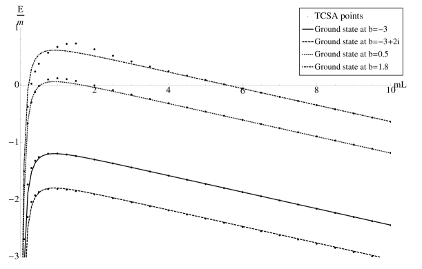
Figure 4: Ground state energies with Lüscher corrections and the TCSA ground state points

For $b=-3$ and $b=-3+2i$ we solved the equations (95, 96) iteratively and plot against the TCSA spectrum. This is shown on figure 5.

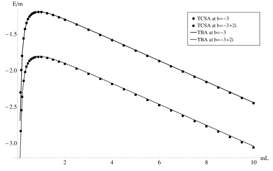
Figure 5: Ground state energies from the defect TBA and the TCSA ground state points

If we choose $b=-3$ the TCSA spectra remains real, and on the scattering theory side, the transmission factor is just a phase for real rapidity and has no poles in the physical strip, so that we do not expect any defect bound-states.

The DTBA equations can be generalised to include the excited states but instead we used a simpler approximate method which is nevertheless accurate for volumes that are not too small. In finite (but not too small) volumes the solutions of the Bethe-Yang equations,

$$e^{iL\sinh\theta_{i}}T_{-}\left(\theta_{i}\right)\prod_{j\neq i}S\left(\theta_{i}-\theta_{j}\right)=1\qquad;\quad i=1,\dots,n$$ (103)

give a good approximation to the rapidities of the $n$-particle state. From these one can easily calculate the energy of the $n$-particle state. As at $b=-3$ the transmission factor is just a phase, we can take the logarithm of these equations, which become a system of real algebraic equation with $n$ integer parameters called the Bethe-Yang quantum numbers. We solved these equations numerically in the case of one and two particles, for the smallest Bethe-Yang quantum numbers, and plotted the resulting energies together with the modified TCSA spectra which can be obtained from the original spectra by subtracting the values of the ground state – see Figure 6.

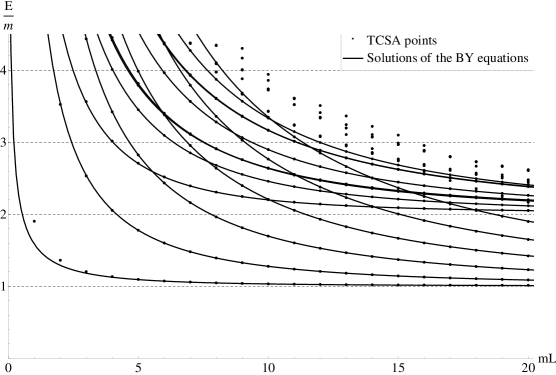
Figure 6: The TCSA spectra together with the solutions of the Bethe Yang equations at $b=-3$.

We should notice that at $b=-3$, the two transmission factors $T_{-}$ and $T_{+}$ are identical, so that we have exact parity-symmetry in this case: the right-moving particle has the same energy as the left-moving. This can be seen in the numerical spectra: all one-particle Bethe-Yang lines and the corresponding TCSA points have multiplicity two. Among the two-particle Bethe-Yang lines, and the corresponding TCSA points, the only lines with multiplicity one are those that correspond to parity-invariant sets of momenta; the others have multiplicity two.

If we choose $b=-3+\alpha i$, with real $\alpha$, the transmission factor remains a phase, and the TCSA spectrum is real. The Bethe-Yang equations become a system of real algebraic equations which can be solved numerically for different quantum numbers. We solved them at the $b=-3+2i$, and plotted the resulting energies in Figure 7 for the smallest quantum numbers in the case of one and two particles, together with the TCSA points. For $mL>5$ every Bethe-Yang line fits the TCSA points. For smaller volumes, due to finite size corrections, there is a mismatch, mainly for the lowest energy lines.

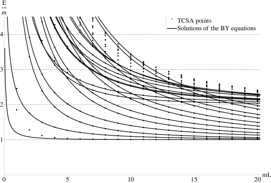
Figure 7: The TCSA spectra together with the solutions of the Bethe-Yang equations at $b=-3+2i$

However it is not true any more that the two transmission factors are identical, the parity-symmetry is broken. Due to this fact, the two-fold degeneracy of the states which was valid for $b=-3$ is broken; thus for $b=-3+i\alpha$ every Bethe-Yang line and the corresponding TCSA points have multiplicity one.

If we choose $\Re\mathrm{e}\left(b\right)\neq-3$, the transmission factors are not just phases any more, and the TCSA spectrum becomes complex as well. If we take the logarithm of the Bethe-Yang equations, they become a system of algebraic equations of complex quantities, each equation holds for both the real and the imaginary part. In the following we plot only the real part as it contains the real vacuum and the boundary bound-states.

According to [10] in different domains of the parameter $b$, the transmission factor $T_{+}$ has poles, and we have defect bound states in infinite volume. In the domain $b\in\left[-1,1\right]$ we expect one defect bound state, and if $b\in\left[1,2\right]$ we expect two. The infinite volume defect energies are given as

$$\epsilon_{1}=m\cos\left(\frac{\pi}{6}\left(b+1\right)\right)\qquad;\quad\epsilon_{2}=m\cos\left(\frac{\pi}{6}\left(b-1\right)\right)$$ (104)

One of the values we have chosen, $b=0.5$, corresponds to a system where we expect a single defect bound state in infinite volume. In finite volume, a defect bound state corresponds to a solution of the Bethe-Yang equations with purely imaginary rapidity. For $mL>5.5$, we in fact find two solutions, one which asymptotically approaches the defect bound state energy in infinite volume, and one which approaches a free massive particle state. For smaller volumes, these converge and meet at $mL\sim 5.5$ and for smaller volumes there are no purely imaginary solutions to the Bethe-Yang equations and indeed the DTCSA has complex spectrum and is consistent with complex rapidity solutions.

We can identify the one and two particle states as the solutions of the Bethe-Yang equations for complex rapidities. In case of the two-particle Bethe-Yang equations there are two kinds of such solutions: one where none of the rapidities are purely imaginary, and one where one of these rapidities is purely imaginary. This latter case corresponds in infinite volume to one particle scattering on the excited defect i.e. a defect with one particle bound on it. The two particle Bethe-Yang equations with one purely imaginary rapidity have solutions only for larger volumes, $mL>7$, but we have to remember that the Bethe-Yang equations are not exact, in small volumes the vacuum polarisation effects become considerable, and we can trust these solutions only for these larger volumes.

We plotted the TCSA spectra together with the solutions of the Bethe-Yang equations for small quantum numbers: The one-particle solutions with purely imaginary rapidities for $mL>5$, the one-particle solutions with non-purely imaginary rapidities, the two-particle solutions with one imaginary rapidity for $mL>7$, and the two particle solutions for non-purely imaginary rapidities. The Bethe-Yang lines fits the TCSA points within an error less then one percent.

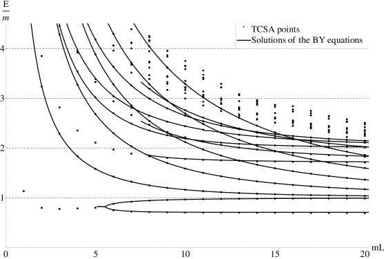
Figure 8: The real part of the TCSA spectra together with the solutions of the Bethe-Yang equations at $b=0.5$

If we choose $b=1.8$ we expect two defect bound state at infinite volume. In finite volume, the corresponding states are the solutions of the one-particle Bethe-Yang equations for purely imaginary rapidities. These equations have solutions only for $mL>3$, for smaller volumes the rapidities have non-zero real part. The corresponding TCSA points are real for $mL>3$, but for smaller volumes these points become complex. But for $mL<5$ the Bethe-Yang lines don’t fit the TCSA points because of the finite size corrections. We also solved the one-particle Bethe-Yang equation for non-imaginary rapidities as well.

We can also identify the two-particle states solving the Bethe-Yang equations. Similarly to the case of $b=0.5$ we have solutions where none of the rapidities are imaginary, and solutions where one of them is purely imaginary. Generally we have two solutions in the latter case corresponding, in infinite volume, to one particle scattering on an excited defect, but at $b=1.8$ we have two of them. These equations for imaginary rapidity don’t have a solution for every volume, this also shows that in small volumes the Bethe-Yang equations are not exact, and one should take into account the vacuum polarisation effects. We plotted the energies of the solutions of the Bethe-Yang equation only in that domain, where these solutions exist.

The energy lines of the solutions of the Bethe-Yang equations fits the TCSA point within $4-5\,\%$ for volumes $mL>5$.

Figure 9: The real part of the TCSA spectra together with the solutions of the Bethe-Yang equations at $b=1.8$. The ground state and the boundary bound-states are real.

8 Conclusion

We have carried out a detailed investigation of the integrable defects in the scaling Lee-Yang model. Our approach is based on the perturbed CFT point of view. Thus, as a starting point, we solved the defect Lee-Yang model by calculating all of its structure constants. This is the first defect conformal field theory solved at such an explicit level.

We then determined the one parameter family of integrable perturbations by using defect conformal perturbation theory. Our findings, (64), agree with the results of Runkel in [22] obtained from an alternative analysis.

We matched the parameters of this UV description to the parameters of the IR scattering theory found in [10] by fusing the defect to the boundary and using the boundary UV-IR relation [24].

We developed the defect truncated conformal space approach to calculate the finite size spectrum of the model and performed various numerical tests. In particular, we verified the UV-IR relation, the transmission factors and the bound-state spectrum of [10]. This was done by comparing the numerical spectrum to the finite size correction determined by the Bethe-Yang equations. We also checked the defect energy contributions and the leading Lüscher corrections to the vacuum energy. These provide convincing evidence for both our solution of the conformal defect Lee-Yang model and for the bootstrap results in [10].

The Lee-Yang theory is a non-unitary theory, nevertheless its spectrum with periodic boundary condition is real. This is due to the PT-symmetry of the model. Introducing defect perturbations we maintain this symmetry but we obtained real spectrum only for real coupling constants. For purely imaginary defect perturbations only the ground state and the defect bound-states were real. This might be related to the fact that these states themselves are P-symmetric, contrary to the rest of the spectrum.

It is worth pointing out that although we write the chiral defect fields as $\varphi$ and $\bar{\varphi}$ and their couplings as $\mu$ and $\bar{\mu}$, the fields are actually real, self-conjugate fields and it is no surprise that we only recovered a real spectrum for $\mu$ and $\bar{\mu}$ both real.

Our developments provide a firm basis to proceed with further work on the defect Lee-Yang model. For example, based on the infinite volume defect form factors [25], one could establish the theory of finite volume defect form factors. These results could then be checked directly by our DTCSA method. This will be the subject of a forthcoming paper.

It will also be interesting to investigate the full space of non-integrable perturbations of the defect, both in the massless and massive cases, using the DTCSA method. Previous investigations of defect perturbations have been limited to the massless case (see eg [26]) and have yielded interesting results for the space of RG flows including flows from purely transmitting defects to purely reflecting defects. A similarly interesting picture is expected for the space of RG flows in the massive Lee-Yang model.

The Lee-Yang model is the simplest conformal field theory, which we solved explicitly in the presence of a topological defect. Our analysis is quite general, however and can be easily generalized to any minimal model, as their topological defects are already classified [21]. These models then could be perturbed and the integrable perturbations classified.

Acknowledgements

We thank Ferenc Wágner for collaboration at an early stage of the project, Gábor Takács and Francesco Buccheri for discussions. GMTW would like to thank Ingo Runkel for discussions, ELTE for hospitality while some of this research was carried out and STFC for partial support under grant ST/J002798/1. Z. Bajnok and L. Holló was supported by OTKA K81461 and by an MTA Lendület grant.

Appendix A Structure constants of the defect Lee-Yang model

In this section we solve the sewing relations for the defect conformal Lee-Yang model and determine all the structure constants. Motivated by TCSA considerations we place the defect at $y=0$ and $x>0$ with $z=x+iy$. We start with the description of the relevant conformal blocks.

The Virasoro algebra with $c=-\frac{22}{5}$ contains only one irredicble highest weight module with non-vanishing highest weight $h=-\frac{1}{5}$. This module contains a singular vector at level 2

$$\left(L_{-1}^{2}-\frac{2}{5}L_{-2}\right)|h\rangle=0$$ (105)

which leads to differential equations for the chiral correlations functions (conformal blocks). Let us denote the chiral field with weight $h$ by $\phi$. The matrix elements of $\phi(z)$ between highest weight states have the following coordinate dependence:

$$\langle 0|\phi(z)|0\rangle=0\quad;\quad\langle 0|\phi(z)|h\rangle\propto z^{-2h}\quad;\quad\langle h|\phi(z)|0\rangle\propto 1\quad;\quad\langle h|\phi(z)|h\rangle\propto z^{-h}$$ (106)

The matrix elements of $\phi(1)\phi(z)$ are proportional to

$$\langle 0|\phi(1)\phi(z)|0\rangle\propto(1-z)^{-2h}\;;\quad\langle 0|\phi(1)\phi(z)|h\rangle\propto(z(1-z))^{-h}\;;\quad\langle h|\phi(1)\phi(z)|0\rangle\propto(1-z)^{-h}$$ (107)

finally from the decoupling of the singular vector we obtain a second order hypergeometric differential equation, which can be solved as

$$\langle h|\phi(1)\phi(z)|h\rangle=c_{1}f_{1}(z)+c_{2}f_{2}(z)$$ (108)

where

$$f_{1}(z)=(z(1-z))^{-h}\,_{2}F_{1}({\scriptstyle\frac{1}{5},\frac{2}{5};\frac{4}{5}}|z)\quad;\qquad f_{2}(z)=(z^{2}(1-z))^{-h}\,_{2}F_{1}({\scriptstyle\frac{2}{5},\frac{3}{5};\frac{6}{5}}|z)$$ (109)

are the canonical solutions around $z\to 0$, i.e. $f_{1}(z)=z^{-h}(1+a_{1}z+\dots)$ and $f_{2}(z)=z^{-2h}(1+a_{2}z+\dots)$. There is a canonical basis around $z\to 1$, too:

$$\langle h|\phi(1)\phi(z)|h\rangle=\tilde{c}_{1}g_{1}(z)+\tilde{c}_{2}g_{2}(z)$$ (110)

such that $g_{1}(z)=(1-z)^{-h}(1+\tilde{a}_{1}(1-z)+\dots)$ and $g_{2}(z)=(1-z)^{-2h}(1+\tilde{a}_{2}(1-z)+\dots)$. As both are solutions of the same differential equations they can be expressed in terms of each other as

$$f_{i}(z)=\Gamma_{ij}g_{j}(z)$$ (111)

with

$$\Gamma_{11}=-\Gamma_{22}=\beta^{-2}\;,\;\;\Gamma_{12}=-\beta^{-2}\alpha^{-2}\;,\;\;\Gamma_{21}=\alpha^{2}$$ (112)

where we use

$$\alpha=\sqrt{\frac{\Gamma(\frac{1}{5})\Gamma(\frac{6}{5})}{\Gamma(\frac{3}{5})\Gamma(\frac{4}{5})}}\quad;\quad\beta=\sqrt{\frac{2}{1+\sqrt{5}}}=\frac{1}{\sqrt{\eta+\eta^{-1}}}\quad;\quad\eta=e^{\frac{i\pi}{5}}\quad;\quad\rho=e^{\frac{i\pi}{5}}$$ (113)

Bulk structure constants

The bulk operators are in a one-to-one correspondence with the bulk Hilbert space: $V_{0}\otimes\bar{V}_{0}+V_{1}\otimes\bar{V}_{1}$ and the structure constants can be calculated in this theory. Let us denote the $(h,h)$ field by $\Phi(z,\bar{z})$. It has the OPE

$$\Phi(z,\bar{z})\Phi(0,0)=C_{\Phi\Phi}^{\mathbb{I}}(z\bar{z})^{2/5}(\mathbb{I}+\dots)+C_{\Phi\Phi}^{\Phi}(z\bar{z})^{1/5}(\Phi(0,0)+\dots)$$ (114)

The four point function can be written in the two canonical bases as

$$\langle\Phi|\Phi(1,1)\Phi(z,\bar{z})|\Phi\rangle=a_{ij}f_{i}(z)f_{j}(\bar{z})=\tilde{a}_{ij}g_{i}(z)g_{j}(\bar{z})$$ (115)

From the two different evaluation of the OPEs we can extract

$$a_{11}=\tilde{a}_{11}=C_{\Phi\Phi}^{\mathbb{I}}\left(C_{\Phi\Phi}^{\Phi}\right)^{2}\quad;\quad a_{22}=\tilde{a}_{22}=\left(C_{\Phi\Phi}^{\mathbb{I}}\right)^{2}$$ (116)

Using the coefficient for the change of basis we obtain:

$$C_{\Phi\Phi}^{\Phi}=\sqrt{-C_{\Phi\Phi}^{\mathbb{I}}}\alpha^{2}\beta$$ (117)

As the three point function can be written as

$$\langle\Phi|\Phi(1,1)|\Phi\rangle=C_{\Phi\Phi\Phi}=C_{\Phi\Phi}^{\mathbb{I}}C_{\Phi\Phi}^{\Phi}$$ (118)

reality of $\Phi^{\dagger}=\Phi$ requires real $C_{\Phi\Phi\Phi}$. We achieve this by choosing the normalization as

$$C_{\Phi\Phi}^{\mathbb{I}}=-1\qquad;\qquad C_{\Phi\Phi}^{\Phi}=\alpha^{2}\beta=1.91131...$$ (119)

Defect Hilbert space

The defect Hilbert space is given by $V_{1}\otimes\bar{V}_{0}+V_{0}\otimes\bar{V}_{1}+V_{1}\otimes\bar{V}_{1}$. (It is like taking the fusion product of a chiral field with all bulk fields). The primary fields with weights $(h,0)$, $(0,h)$ and $(h,h)$ will be denoted as $d$, $\bar{d}$ and $D$, respectively. We normalize them as

$$\langle d|d\rangle=C_{dd}^{\mathbb{I}}=\langle\bar{d}|\bar{d}\rangle=C_{\bar{d}\bar{d}}^{\mathbb{I}}=1\quad;\qquad\langle D|D\rangle=C_{DD}^{\mathbb{I}}=-1$$ (120)

and all other matrix elements are vanishing.

Defect operators

The defect operators are in one-to-one correspondence to the Hilbert space containing two defects: $V_{0}\otimes\bar{V}_{0}+V_{1}\otimes\bar{V}_{0}+V_{0}\otimes\bar{V}_{1}+2\cdot V_{1}\otimes\bar{V}_{1}$. (It is like taking the fusion product of a chiral field with the defect Hilbert space). The primary fields and weights are as follows: $\mathbb{I}$ with $(0,0)$, $\varphi$ and $\bar{\varphi}$ with $(h,0)$ and $(0,h)$, finally we have two fields $\Phi_{+}$ and $\Phi_{-}$ both with weights $(h,h)$. We will choose them as the lower/upper limits of the bulk field on the defect

$$\Phi_{\pm}(x)=\lim_{y\to\mp 0}\Phi(z,\bar{z})\quad;\qquad z=x+iy$$ (121)

As the map from the cylinder to the plane is $z=e^{-i\frac{2\pi}{L}\zeta}$ the left/right limit on the cylinder corresponded to the lower/upper limit on the plane. This implies the normalization of the fields

$$C_{\Phi_{+}\Phi_{+}}^{\mathbb{I}}=C_{\Phi_{-}\Phi_{-}}^{\mathbb{I}}=C_{\Phi\Phi}^{\mathbb{I}}=-1$$ (122)

In order to maintain reality of the chiral fields we normalize them as

$$C_{\varphi\varphi}^{\mathbf{\mathbb{I}}}=C_{\bar{\varphi}\bar{\varphi}}^{\mathbf{\mathbb{I}}}=-1$$ (123)

As the fields are real, complex conjugation $z\leftrightarrow\bar{z}$ will make the changes:

$$z\leftrightarrow\bar{z}\quad,\qquad\Phi_{\pm}\leftrightarrow\Phi_{\mp}\quad;\qquad\varphi\leftrightarrow\bar{\varphi}$$ (124)

Defect OPEs

The defect operators have the following operator product expansions

$$\varphi(z)\varphi(w) = C_{\varphi\varphi}^{\mathbb{I}}|z-w|^{2/5}+C_{\varphi\varphi}^{\varphi}|z-w|^{1/5}\varphi(w)\dots$$ (125)

$$\varphi(z)\bar{\varphi}(w) = C_{\varphi\bar{\varphi}}^{\Phi_{+}}\Phi_{+}(w)+C_{\varphi\bar{\varphi}}^{\Phi_{-}}\Phi_{-}(w)\dots$$ (126)

$$\bar{\varphi}(z)\varphi(w) = C_{\bar{\varphi}\varphi}^{\Phi_{+}}\Phi_{+}(w)+C_{\bar{\varphi}\varphi}^{\Phi_{-}}\Phi_{-}(w)\dots$$ (127)

$$\bar{\varphi}(z)\bar{\varphi}(w) = C_{\bar{\varphi}\bar{\varphi}}^{\mathbb{I}}|z-w|^{2/5}+C_{\bar{\varphi}\bar{\varphi}}^{\bar{\varphi}}|z-w|^{1/5}\bar{\varphi}(w)\dots$$ (128)

$$\Phi_{+}(z)\Phi_{+}(w) = C_{\Phi_{+}\Phi_{+}}^{\mathbf{\mathbb{I}}}|z-w|^{4/5}+C_{\Phi\Phi}^{\Phi}|z-w|^{2/5}\Phi_{+}(w)\dots$$ (129)

$$\Phi_{+}(z)\Phi_{-}(w) = C_{\Phi_{+}\Phi_{-}}^{\mathbf{\mathbb{I}}}|z-w|^{4/5}+C_{\Phi_{+}\Phi_{-}}^{\varphi}|z-w|^{3/5}\varphi(w)+C_{\Phi_{+}\Phi_{-}}^{\bar{\varphi}}|z-w|^{3/5}\bar{\varphi}(w)+$$ (130)

$$+C_{\Phi_{+}\Phi_{-}}^{\Phi_{+}}|z-w|^{2/5}\Phi_{+}(w)+C_{\Phi_{+}\Phi_{-}}^{\Phi_{-}}|z-w|^{2/5}\Phi_{-}(w)\dots$$

$$\Phi_{-}(z)\Phi_{+}(w) = C_{\Phi_{-}\Phi_{+}}^{\mathbf{\mathbb{I}}}|z-w|^{4/5}+C_{\Phi_{-}\Phi_{+}}^{\varphi}|z-w|^{3/5}\varphi(w)+C_{\Phi_{-}\Phi_{+}}^{\bar{\varphi}}|z-w|^{3/5}\bar{\varphi}(w)+$$ (131)

$$+ C_{\Phi_{-}\Phi_{+}}^{\Phi_{+}}|z-w|^{2/5}\Phi_{+}(w)+C_{\Phi_{-}\Phi_{+}}^{\Phi_{-}}|z-w|^{2/5}\Phi_{-}(w)\dots$$

$$\Phi_{-}(z)\Phi_{-}(w) = C_{\Phi_{-}\Phi_{-}}^{\mathbf{\mathbb{I}}}|z-w|^{4/5}+C_{\Phi\Phi}^{\Phi}|z-w|^{2/5}\Phi_{-}(w)\dots$$ (132)

where we have exploited the relation of $\Phi$ and $\Phi_{\pm}$ to write $C_{\Phi_{+}\Phi_{+}}^{\Phi_{+}}=C_{\Phi_{-}\Phi_{-}}^{\Phi_{-}}=C_{\Phi\Phi}^{\Phi}$.

Matrix elements of $\varphi$ and $\bar{\varphi}$

The non-vanishing matrix elements of the defect operators at $z=1$ on the highest weight basis $(d,D,\bar{d})$ can be calculated from the matrix form of the OPEs

$$\hat{\varphi}=\left(\begin{array}[]{ccc}C_{\varphi d}^{d}&0&0\\ 0&C_{\varphi D}^{D}&C_{\varphi\bar{d}}^{D}\\ 0&C_{\varphi D}^{\bar{d}}&0\end{array}\right)\quad;\qquad\hat{\bar{\varphi}}=\left(\begin{array}[]{ccc}0&C_{\bar{\varphi}D}^{d}&0\\ C_{\bar{\varphi}d}^{D}&C_{\bar{\varphi}D}^{D}&0\\ 0&0&C_{\bar{\varphi}\bar{d}}^{\bar{d}}\end{array}\right)$$ (133)

In order to get the matrix elements we multiply with the normalization of states: $\langle i|\varphi|j\rangle=C_{\varphi j}^{k}C_{ik}^{\mathbb{I}}$. Since complex conjugation relates the two by changing $d\leftrightarrow\bar{d}$ we determine only the first. Analyzing carefully the OPEs we can express the various matrix elements of $\varphi(1)\varphi(z)$ in terms of the chiral blocks:

$$\langle d|\varphi(1)\varphi(z)|d\rangle=\left(C_{\varphi d}^{d}\right)^{2}f_{1}(z)=C_{\varphi\varphi}^{\mathbf{\mathbb{I}}}g_{2}(z)+C_{\varphi\varphi}^{\varphi}C_{\varphi d}^{d}g_{1}(z)$$ (134)

$$-\langle D|\varphi(1)\varphi(z)|D\rangle=\left(C_{\varphi D}^{D}\right)^{2}f_{1}(z)+C_{\varphi D}^{\bar{d}}C_{\varphi\bar{d}}^{D}f_{2}(z)=C_{\varphi\varphi}^{\mathbf{\mathbb{I}}}g_{2}(z)+C_{\varphi\varphi}^{\varphi}C_{\varphi D}^{D}g_{1}(z)$$ (135)

$$\langle\bar{d}|\varphi(1)\varphi(z)|\bar{d}\rangle=C_{\varphi\bar{d}}^{D}C_{\varphi D}^{\bar{d}}(1-z)^{-2h}=C_{\varphi\varphi}^{\mathbf{\mathbb{I}}}(1-z)^{-2h}$$ (136)

$$\langle\bar{d}|\varphi(1)\varphi(z)|D\rangle=C_{\varphi D}^{D}C_{\varphi D}^{\bar{d}}z^{-h}(1-z)^{-h}=C_{\varphi\varphi}^{\varphi}C_{\varphi D}^{\bar{d}}z^{-h}(1-z)^{-h}$$ (137)

$$-\langle D|\varphi(1)\varphi(z)|\bar{d}\rangle=C_{\varphi\bar{d}}^{D}C_{\varphi D}^{D}(1-z)^{-h}=C_{\varphi\varphi}^{\varphi}C_{\varphi\bar{d}}^{D}(1-z)^{-h}$$ (138)

From which it easily follows that $C_{\varphi\bar{d}}^{D}C_{\varphi D}^{\bar{d}}=C_{\varphi\varphi}^{\mathbf{\mathbb{I}}}=-1$ and $C_{\varphi D}^{D}=C_{\varphi\varphi}^{\varphi}$. Furthermore, we found that

$$C_{\varphi\varphi}^{\varphi}=C_{\varphi D}^{D}=\alpha\beta^{-1}\quad\quad C_{\varphi d}^{d}=\alpha\beta$$ (139)

We can write the analogous equations by changing $d\leftrightarrow\bar{d}$ and $\varphi\leftrightarrow\bar{\varphi}$. The result is

$$C_{\bar{\varphi}d}^{D}C_{\bar{\varphi}D}^{d}=C_{\bar{\varphi}\bar{\varphi}}^{\mathbf{\mathbb{I}}}=-1\quad;\quad C_{\bar{\varphi}\bar{\varphi}}^{\bar{\varphi}}=C_{\bar{\varphi}D}^{D}=\alpha\beta^{-1}\quad\quad C_{\bar{\varphi}\bar{d}}^{\bar{d}}=\alpha\beta$$ (140)

although we could have changed the sign of $\bar{\varphi}$ which is still a solution.

Matrix elements of $\Phi_{\pm}$

The matrix elements of $\Phi_{+}$ and $\Phi_{-}$ are related either by complex conjugation or by analyzing the matrix elements of the bulk field $\Phi(z,\bar{z})$ and taking the two limits $\theta\to 0$ and $\theta\to 2\pi$ in

$$\langle i|\Phi(z,\bar{z})|j\rangle=\langle i|\Phi_{-}(1)|j\rangle z^{h_{i}-h_{j}-h}\bar{z}^{\bar{h}_{i}-\bar{h}_{j}-h}\quad;\qquad z=re^{i\theta}$$ (141)

This implies

$$\langle i|\Phi_{-}(1)|j\rangle=e^{2\pi i(h_{i}-\bar{h}_{i}-(h_{j}-\bar{h}_{j}))}\langle i|\Phi_{+}(1)|j\rangle\qquad;\qquad\xi=e^{i\frac{2\pi}{5}}$$ (142)

The $\Phi_{\pm}(1)$ matrix elements can be parametrised as

$$\hat{\Phi}_{-}=\left(\begin{array}[]{ccc}0&C_{\Phi_{-}D}^{d}&C_{\Phi_{-}\bar{d}}^{d}\\ C_{\Phi_{-}d}^{D}&C_{\Phi_{-}D}^{D}&C_{\Phi_{-}\bar{d}}^{D}\\ C_{\Phi_{-}d}^{\bar{d}}&C_{\Phi_{-}D}^{\bar{d}}&0\end{array}\right)\quad;\qquad\hat{\Phi}_{+}=\left(\begin{array}[]{ccc}0&\xi^{-1}C_{\Phi_{-}D}^{d}&\xi^{-2}C_{\Phi_{-}\bar{d}}^{d}\\ \xi C_{\Phi_{-}d}^{D}&C_{\Phi_{-}D}^{D}&\xi^{-1}C_{\Phi_{-}\bar{d}}^{D}\\ \xi^{2}C_{\Phi_{-}d}^{\bar{d}}&\xi C_{\Phi_{-}D}^{\bar{d}}&0\end{array}\right)$$ (143)

These matrix elements can be determined from the correlation functions

$$\langle i|\varphi(1)\bar{\varphi}(z)|j\rangle=C_{il}^{\mathbb{I}}C_{\varphi k}^{l}C_{\bar{\varphi}j}^{k}z^{\bar{h}_{i}-\bar{h}_{j}-h}=C_{il}^{\mathbb{I}}(C_{\varphi\bar{\varphi}}^{\Phi_{-}}C_{\Phi_{-}j}^{l}+C_{\varphi\bar{\varphi}}^{\Phi_{+}}C_{\Phi_{+}j}^{l})z^{\bar{h}_{i}-\bar{h}_{j}-h}$$ (144)

In matrix notation they read as

$$\hat{\varphi}\hat{\bar{\varphi}}=C_{\varphi\bar{\varphi}}^{\Phi_{-}}\hat{\Phi}_{-}+C_{\varphi\bar{\varphi}}^{\Phi_{+}}\hat{\Phi}_{+}$$ (145)

By solving the equations we found a one parameter family of solutions. We fixed this freedom by choosing

$$C_{\varphi D}^{\bar{d}}=C_{\bar{\varphi}D}^{d}=1\quad;\qquad C_{\varphi\bar{d}}^{D}=C_{\bar{\varphi}d}^{D}=-1$$ (146)

The rest of the coefficients are

$$C_{\Phi_{+}\Phi_{+}}^{\Phi_{+}}=C_{\Phi_{-}\Phi_{-}}^{\Phi_{-}}=\alpha^{2}\beta\quad;\qquad C_{\varphi d}^{d}=C_{\bar{\varphi}\bar{d}}^{\bar{d}}=\alpha\beta$$ (147)

$$C_{\varphi\bar{\varphi}}^{\Phi_{-}}=C_{\bar{\varphi}\varphi}^{\Phi_{+}}=\frac{\beta^{-1}}{1+\eta^{-1}}=\frac{\rho}{\sqrt[4]{5}}\quad;\qquad C_{\varphi\bar{\varphi}}^{\Phi_{+}}=C_{\bar{\varphi}\varphi}^{\Phi_{-}}=\frac{\beta^{-1}}{1+\eta}=\frac{\rho^{-1}}{\sqrt[4]{5}}$$ (148)

$$C_{\Phi_{-}D}^{d}=C_{\Phi_{+}D}^{\bar{d}}=\alpha\eta\quad;\qquad C_{\Phi_{-}D}^{\bar{d}}=C_{\Phi_{+}D}^{d}=\alpha\eta^{-1}$$ (149)

$$C_{\Phi_{-}\bar{d}}^{d}=C_{\Phi_{+}d}^{\bar{d}}=-\eta^{2}\beta^{-1}\quad;\qquad C_{\Phi_{-}d}^{\bar{d}}=C_{\Phi_{+}\bar{d}}^{d}=-\eta^{-2}\beta^{-1}$$ (150)

$$C_{\Phi_{-}d}^{D}=C_{\Phi_{+}\bar{d}}^{D}=-\eta^{-1}\alpha\quad;\qquad C_{\Phi_{-}\bar{d}}^{D}=C_{\Phi_{+}d}^{D}=-\eta\alpha$$ (151)

$$C_{\Phi_{-}D}^{D}=C_{\Phi_{+}D}^{D}=\alpha^{2}\beta^{-1}\quad;\qquad C_{\Phi_{-}\Phi_{+}}^{\mathbb{I}}=C_{\Phi_{+}\Phi_{-}}^{\mathbb{I}}=\left(1+\beta^{-2}\right)$$ (152)

$$C_{\Phi_{-}\Phi_{+}}^{\Phi_{-}}=C_{\Phi_{+}\Phi_{-}}^{\Phi_{+}}=C_{\Phi_{-}\Phi_{+}}^{\Phi_{+}}=C_{\Phi_{+}\Phi_{-}}^{\Phi_{-}}=\beta^{-1}\alpha^{2}$$ (153)

$$C_{\Phi_{-}\Phi_{+}}^{\varphi}=C_{\Phi_{+}\Phi_{-}}^{\bar{\varphi}}=-\rho\alpha\beta^{-2}\sqrt[4]{5}\quad;\quad C_{\Phi_{-}\Phi_{+}}^{\bar{\varphi}}=C_{\Phi_{+}\Phi_{-}}^{\varphi}=-\rho^{-1}\alpha\beta^{-2}\sqrt[4]{5}$$ (154)

$$C_{\Phi_{-}\bar{\varphi}}^{\varphi}=C_{\Phi_{+}\varphi}^{\bar{\varphi}}=C_{\bar{\varphi}\Phi_{+}}^{\varphi}=C_{\varphi\Phi_{-}}^{\bar{\varphi}}=-\beta^{-1}\eta$$ (155)

$$C_{\bar{\varphi}\Phi_{-}}^{\varphi}=C_{\varphi\Phi_{+}}^{\bar{\varphi}}=C_{\Phi_{+}\bar{\varphi}}^{\varphi}=C_{\Phi_{-}\varphi}^{\bar{\varphi}}=-\beta^{-1}\eta^{-1}$$ (156)

$$C_{\Phi_{-}\varphi}^{\Phi_{-}}=C_{\Phi_{+}\bar{\varphi}}^{\Phi_{+}}=C_{\bar{\varphi}\Phi_{-}}^{\Phi_{-}}=C_{\varphi\Phi_{+}}^{\Phi_{+}}=\frac{\alpha}{2}\left(\left(\beta+\beta^{-1}\right)-i\frac{1}{\sqrt[4]{5}}\right)=\frac{\alpha}{2}\rho^{-1}\sqrt{\frac{6}{\sqrt{5}}+2}$$ (157)

$$C_{\Phi_{-}\bar{\varphi}}^{\Phi_{-}}=C_{\Phi_{+}\varphi}^{\Phi_{+}}=C_{\varphi\Phi_{-}}^{\Phi_{-}}=C_{\bar{\varphi}\Phi_{+}}^{\Phi_{+}}=\frac{\alpha}{2}\left(\left(\beta+\beta^{-1}\right)+i\frac{1}{\sqrt[4]{5}}\right)=\frac{\alpha}{2}\rho\sqrt{\frac{6}{\sqrt{5}}+2}$$ (158)

$$C_{\varphi\Phi_{+}}^{\Phi_{-}}=C_{\bar{\varphi}\Phi_{-}}^{\Phi_{+}}=C_{\Phi_{+}\bar{\varphi}}^{\Phi_{-}}=C_{\Phi_{-}\varphi}^{\Phi_{+}}=\frac{\alpha\beta}{2}\left(1+i\left(\beta-\beta^{-1}\right)\frac{1}{\sqrt[4]{5}}\right)=\frac{\alpha}{2}\rho^{-1}\sqrt{\frac{6}{\sqrt{5}}-2}$$ (159)

$$C_{\bar{\varphi}\Phi_{+}}^{\Phi_{-}}=C_{\varphi\Phi_{-}}^{\Phi_{+}}=C_{\Phi_{+}\varphi}^{\Phi_{-}}=C_{\Phi_{-}\bar{\varphi}}^{\Phi_{+}}=\frac{\alpha\beta}{2}\left(1-i\left(\beta-\beta^{-1}\right)\frac{1}{\sqrt[4]{5}}\right)=\frac{\alpha}{2}\rho\sqrt{\frac{6}{\sqrt{5}}-2}$$ (160)

In matrix notation

$$\hat{\Phi}_{-}=\left(\begin{array}[]{ccc}0&\eta\alpha&-\eta^{2}\beta^{-1}\\ -\eta^{-1}\alpha&\alpha^{2}\beta^{-1}&-\eta^{1}\alpha\\ -\eta^{-2}\beta^{-1}&\eta^{-1}\alpha&0\end{array}\right)\;;\quad\hat{\Phi}_{+}=\left(\begin{array}[]{ccc}0&\eta^{-1}\alpha&-\eta^{-2}\beta^{-1}\\ -\eta^{1}\alpha&\alpha^{2}\beta^{-1}&-\eta^{-1}\alpha\\ -\eta^{2}\beta^{-1}&\eta^{1}\alpha&0\end{array}\right)$$ (161)

Appendix B Perturbation theory calculations.

In this Appendix we calculate the bulk-defect operator expansion induced by simultaneous bulk, chiral and anti-chiral defect perturbations. From this we can easily calculate the jump in $T$ and $\bar{T}$ across the defect.

Operator equations are local, which are understood within correlators in the perturbed theory. This means we require them in the weak sense for any of their matrix elements. For technical reasons we present the calculation here for matrix elements in the theory where two defect lines are included, i.e. when there is a one-to-one correspondence between defect operators and vectors of the Hilbert space. We place the defect at $x=0$ and sometimes write out explicitly that fields depend on $z=x+iy$, such as like $\varphi(iy)$.

There are singularities in the perturbative expansion of correlation functions including $T(0)$ coming from integration over the boundary perturbation. The solution is to consider instead the regularised field

$$T_{R}(0)=T(0)+\frac{a\mu}{\epsilon}\varphi(0)\;.$$ (162)

The constant $a$ can be fixed by requiring the bulk-defect OPE of $T(x)$ to be

$$e^{-\delta S}T(x)=e^{-\delta S}T_{R}(0)+O(x,\mu)\;.$$ (163)

If we sandwich this identity between ${\langle{\varphi}|}$ and ${|0\rangle}$, we get

$${\langle{\varphi}|}\,e^{-\delta S}\,(T(x)-T(0)){|0\rangle}=({a\mu}/\epsilon){\langle{\varphi}|}\,e^{-\delta S}\,\varphi(0){|0\rangle}\;.$$ (164)

We fix $a$ by differentiating both sides with respect to $\mu$ and setting $\mu$ to zero. Since the singularity arises for $\epsilon\to 0$, we can always take $x>\epsilon$, to get

$$a = \epsilon\lim_{R\to\infty}\int_{-R}^{R}\frac{{\langle{\varphi}|}\varphi(iy)(T(x)-T(0)){|0\rangle}}{{\langle{\varphi}|}\varphi(0){|0\rangle}}dy\Big{|}_{\hbox{\tiny cutoff}}$$

$$= \epsilon\lim_{R\to\infty}\int_{-R}^{R}\left(\frac{h}{(x-iy)^{2}}\theta(x^{2}+y^{2}-\epsilon^{2})-\frac{h}{(iy)^{2}}\theta(y^{2}-\epsilon^{2})\right)dy$$

$$= -h\epsilon\lim_{R\to\infty}\left(\int_{-R}^{R}\frac{dy}{(y+ix)^{2}}-\int_{-R}^{-\epsilon}\frac{dy}{y^{2}}-\int_{\epsilon}^{R}\frac{dy}{y^{2}}\right)$$

$$= {2h}\;,$$

where “cutoff” means we need to implement the short-distance cutoff in the perturbative integrals.

Having defined the renormalized field we can now write the general bulk-defect operator expansion for the combined chiral, anti-chiral and bulk perturbations in the case ${x}>0$:

$$T({x})=T_{R}(0)+b^{+}\mu\partial_{y}\varphi(0)+\eta^{+}\lambda\Phi_{+}(0)+\eta^{-}\lambda\Phi_{-}(0)+\mu\bar{\mu}\Big{(}\rho\bar{\varphi}(0)\varphi(0)+\sigma\varphi(0)\bar{\varphi}(0)\Big{)}+\ldots$$ (165)

We will need to find $b^{+}$, the coefficient of $\partial_{y}\varphi(iy)=i\partial\varphi(iy)$. We have $\partial_{y}\varphi(0){|0\rangle}=iL_{-1}{|{\varphi}\rangle}$ and so we find $b^{+}$ by sandwiching

$$T({x})=T_{R}(0)+\cdots+\gamma\mu\partial_{y}\varphi(iy)+\cdots\;,$$

between ${\langle{\psi}|}=-\frac{i}{2h}{\langle{\varphi}|}L_{1}$ and ${|0\rangle}$, differentiating with respect to $\mu$ and setting $\mu\to 0$, giving

$$b^{+} = -\frac{i}{2h}\int{{\langle{\varphi}|}L_{1}\varphi(iy)(T({x})-T(0)){|0\rangle}}/{{\langle{\varphi}|}\varphi\rangle}\;{\mathrm{d}}y\Big{|}_{\hbox{\tiny cutoff}}$$

$$= -i\lim_{R\to\infty}\int_{y=-R}^{R}\left[\left(\frac{h{x}}{({x}-iy)^{2}}+\frac{(1-h)}{{x}-iy}\right)\theta(|{x}-iy|-\epsilon)-\frac{(1-h)}{-iy}\theta(|y|-\epsilon){\mathrm{d}}y\right]$$

$$= -\lim_{R\to\infty}\left[\int_{-R}^{-\epsilon}+\int_{\epsilon}^{R}(1-h)\frac{{\mathrm{d}}y}{y}\right]-\left[\int_{-R}^{R}\left(\frac{ih{x}}{(y+i{x})^{2}}+\frac{1-h}{y+i{x}}\right){\mathrm{d}}y\right]$$

$$= -\lim_{R\to\infty}\left(-(1-h)\log\left(\frac{i{x}+R}{i{x}-R}\right)+ih{x}\left[\frac{1}{R+i{x}}+\frac{1}{R-i{x}}\right]\right)$$

$$= -i\pi(1-h)\;.$$

We will also need $\eta^{+}$, the coefficient of $\Phi_{+}$ appearing in the bulk-defect OPE. This can be found by sandwiching the bulk-defect operator expansion between ${\langle{+}|}$ and ${|0\rangle}$, where the state ${\langle{+}|}$ picks out the contribution from $\Phi(x)$ with positive $x$ —

$${\langle{+}|}\Phi(x){|0\rangle}=1\,\,(x>0)\;,\;\;\;{\langle{+}|}\Phi(x){|0\rangle}=0\,\,(x<0)\;.$$

This state exists so long as $\Phi(x)$ is discontinuous across the defect. The result is

$$\eta^{+}=\lim_{R\to\infty}\int_{U}{\mathrm{d}}^{2}u{\langle{+}|}\Phi(u)(T({x})-T(0)){|0\rangle}\Big{|}_{\hbox{\tiny cutoff}}=\lim_{R\to\infty}\int_{U_{1}}{\mathrm{d}}^{2}u\frac{h}{(u-{x})^{2}}-\int_{U_{2}}{\mathrm{d}}^{2}u\frac{h}{u^{2}}\;,$$

where the integration region $U=\{u\in\mathbb{C}|Re(u)>0,|u|<R\}$, $U_{1}=\{u\in\mathbb{C}|Re(u)>0,|u|<R,|u-x|>\epsilon\}$ and $U_{2}=\{u\in\mathbb{C}|Re(u)>0,\epsilon<|u|<R\}$. The second integral is zero, as can be found by taking $u=re^{i\theta}$. For the first integral, we can take $u={x}+re^{i\theta}$, and then the integration region is approximately given by $U_{3}=\{re^{i\theta}|\epsilon<r<R,r\cos\theta+x>0\}$. The difference between this approximate region and the correct region goes to zero as $R$ goes to infinity. We then find, with $\theta_{0}=\sin^{-1}(x/R)$,

$$\int_{U_{2}}{\mathrm{d}}^{2}u\frac{1}{(u-x)^{2}}\simeq\int_{U_{3}}\frac{{\mathrm{d}}r\,{\mathrm{d}}\theta}{re^{2i\theta}}$$

$$= \int_{r=\epsilon}^{R}\int_{\theta=-\pi/2-\theta_{0}}^{\pi/2+\theta_{0}}\frac{{\mathrm{d}}r\,{\mathrm{d}}\theta}{re^{2i\theta}}+\int_{\theta=-\pi}^{-\pi/2-\theta_{0}}\int_{r=\epsilon}^{-x/\cos\theta}\frac{{\mathrm{d}}r\,{\mathrm{d}}\theta}{re^{2i\theta}}+\int_{\theta=\pi/2+\theta_{0}}^{\pi}\int_{r=\epsilon}^{-x/\cos\theta}\frac{{\mathrm{d}}r\,{\mathrm{d}}\theta}{re^{2i\theta}}$$

$$= \int_{\theta=-\pi/2-\theta_{0}}^{\pi/2+\theta_{0}}e^{-2i\theta}\log(R/\epsilon){\mathrm{d}}\theta+\int_{\theta=-\pi}^{-\pi/2-\theta_{0}}e^{-2i\theta}\log\left(-\frac{x}{\epsilon\cos\theta}\right){\mathrm{d}}\theta$$

$$+\int_{\theta=\pi/2+\theta_{0}}^{\pi}e^{-2i\theta}\log\left(-\frac{x}{\epsilon\cos\theta}\right){\mathrm{d}}\theta$$

$$= \frac{1}{2}\left(2\theta_{0}+\sin(2\theta_{0})-\pi\right)$$

In the limit $R\to\infty$, $\theta_{0}\to 0$ and so $\eta^{+}=-{h\pi}/2\;.$ We can likewise find the remaining coefficients to get the bulk-defect operator expansion, valid for $x>0$,

$$T({x})=T_{R}(0)-i\pi(1-h)\mu\partial_{y}\varphi(0)-\frac{h\pi}{2}\lambda(\Phi_{+}(0)-\Phi_{-}(0))+i\pi h\mu\bar{\mu}\Big{[}\varphi(0),\bar{\varphi}(0)\Big{]}+\ldots$$ (166)

and so we find the jump in $T$ to be

$$\Delta T({x}) = 2\pi i(1{-}h)\mu\,\partial_{y}\varphi(0)-{h\pi}\lambda\,\Delta\Phi(0)-2\pi ih\mu\bar{\mu}\Big{[}\varphi(0),\bar{\varphi}(0)\Big{]}+\ldots$$ (167)

$$\Delta\bar{T}({x}) = -2\pi i(1{-}h)\bar{\mu}\,\partial_{y}\bar{\varphi}(0)-{h\pi}\lambda\,\Delta\Phi(0)-2\pi ih\mu\bar{\mu}\Big{[}\varphi(0),\bar{\varphi}(0)\Big{]}+\ldots$$ (168)

References

- [1] G. Delfino, G. Mussardo, and P. Simonetti. Scattering theory and correlation functions in statistical models with a line of defect. Nucl.Phys., B432:518–550, 1994.
- [2] P. Bowcock, Edward Corrigan, and C. Zambon. Classically integrable field theories with defects. Int.J.Mod.Phys., A19S2:82–91, 2004.
- [3] J.F. Gomes, L.H. Ymai, and A.H. Zimerman. Classical Integrable N=1 and N= 2 Super Sinh-Gordon Models with Jump Defects. J.Phys.Conf.Ser., 128:012004, 2008.
- [4] V. Caudrelier. On a systematic approach to defects in classical integrable field theories. Int.J.Geom.Meth.Mod.Phys., 5:1085–1108, 2008.
- [5] Edward Corrigan and C. Zambon. A New class of integrable defects. J.Phys.A, A42:475203, 2009.
- [6] Jean Avan and Anastasia Doikou. The sine-Gordon model with integrable defects revisited. JHEP, 1211:008, 2012.
- [7] Anastasia Doikou and Nikos Karaiskos. Sigma models in the presence of dynamical point-like defects. Nucl.Phys., B867:872–886, 2013.
- [8] Robert Konik and Andre LeClair. Purely transmitting defect field theories. Nucl.Phys., B538:587–611, 1999.
- [9] P. Bowcock, Edward Corrigan, and C. Zambon. Some aspects of jump-defects in the quantum sine-Gordon model. JHEP, 0508:023, 2005.
- [10] Z. Bajnok and Zs. Simon. Solving topological defects via fusion. Nucl.Phys., B802:307–329, 2008.
- [11] E. Corrigan and C. Zambon. Integrable defects in affine Toda field theory and infinite dimensional representations of quantum groups. Nucl.Phys., B848:545–577, 2011.
- [12] E. Corrigan and C. Zambon. A Transmission matrix for a fused pair of integrable defects in the sine-Gordon model. J.Phys.A, A43:345201, 2010.
- [13] Edward Corrigan and C. Zambon. On purely transmitting defects in affine Toda field theory. JHEP, 0707:001, 2007.
- [14] Ismagil Habibullin and Anjan Kundu. Quantum and classical integrable sine-Gordon model with defect. Nucl.Phys., B795:549–568, 2008.
- [15] Zoltan Bajnok and Ladislav Samaj. Introduction to integrable many-body systems III. Acta Physica Slovaca, 61, No.2:129–271, 2011.
- [16] Z. Bajnok and A. George. From defects to boundaries. Int.J.Mod.Phys., A21:1063–1078, 2006.
- [17] Boris L. Feigin, Tomoki Nakanishi, and Hirosi Ooguri. The Annihilating ideals of minimal models. Int.J.Mod.Phys., A7S1A:217–238, 1992.
- [18] J. F. Fortin, P. Jacob, and P. Mathieu. SM(2,4) fermionic characters and restricted jagged partitions. J. Phys., A38:1699–1710, 2005.
- [19] Werner Nahm, Andreas Recknagel, and Michael Terhoeven. Dilogarithm identities in conformal field theory. Mod. Phys. Lett., A8:1835–1848, 1993.
- [20] Thomas Quella, Ingo Runkel, and Gerard M. T. Watts. Reflection and Transmission for Conformal Defects. JHEP, 04:095, 2007.
- [21] V. B. Petkova and J. B. Zuber. Generalised twisted partition functions. Phys. Lett., B504:157–164, 2001.
- [22] Ingo Runkel. Non-local conserved charges from defects in perturbed conformal field theory. J. Phys., A43:365206, 2010.
- [23] Zoltan Bajnok, Omar el Deeb, and Paul Pearce. The spectrum of the Lee-Yang model in finite volume. To appear.
- [24] Patrick Dorey, Andrew Pocklington, Roberto Tateo, and Gerard Watts. TBA and TCSA with boundaries and excited states. Nucl. Phys., B525:641–663, 1998.
- [25] Zoltan Bajnok and Omar el Deeb. Form factors in the presence of integrable defects. Nucl.Phys., B832:500–519, 2010.
- [26] Marton Kormos, Ingo Runkel, and Gerard M.T. Watts. Defect flows in minimal models. JHEP, 0911:057, 2009.