Mixing-Demixing Phase Diagram for Simple Liquids
in Non-Uniform Electric Fields

Abstract

We deduce the mixing-demixing phase diagram for binary liquid mixtures in an electric field for various electrode geometries and arbitrary constitutive relation for the dielectric constant. By focusing on the behavior of the liquid-liquid interface, we produce simple analytic expressions for the dependence of the interface location on experimental parameters. We also show that the phase diagram contains regions where liquid separation cannot occur under any applied field. The analytic expression for the boundary “electrostatic binodal” line reveals that the regions’ size and shape depend strongly on the dielectric relation between the liquids. Moreover, we predict the existence of an “electrostatic spinodal” line that identifies conditions where the liquids are in a metastable state. We finally construct the phase diagram for closed systems by mapping solutions onto those of an open system via an effective liquid composition. For closed systems at a fixed temperature and mixture composition, liquid separation occurs in a finite “window” of surface potential (or charge density). Larger potentials or charge densities counterintuitively destroy the interface, leading to liquid mixing. These results give valuable guides for experiments by providing easily testable predictions for how liquids behave in non-uniform electric fields.

Phase transitions describe fundamental transformations in substances, where material properties, such as viscosity, refractive index, etc., often dramatically change. These changes are not only mediated by intrinsic thermodynamic variables (temperature, pressure, etc.), but also by external forces (gravitational Moldover1979 , magnetic Asamitsu1995 and electric Landau1957 fields, and shear flows Silberberg1952 ; Nakatani1996 ). Scientific interest in using electric fields to alter the phase behavior spans over half a century and resulted in theories and experiments devoted to the application of uniform fields in dielectric liquid mixtures Landau1957 ; Onuki1995a ; Onuki1995b ; Stepanow2009 ; Debye1965 ; Beaglehole1981 ; Early1992 ; Wirtz1993 ; Orzechowski1999 . Unfortunately, the liquid-field coupling in uniform electric fields is very weak since in such cases variations in the field strength occur as a result of variations in the permittivity of the liquid. As a consequence, theories predict that even minuscule changes to the phase diagram require enormous applied voltages Landau1957 ; Onuki1995a ; Debye1965 .

In contrast, recent theoretical and experimental results reveal that nonuniform fields can effectuate large changes in phase diagrams Tsori2004 ; Marcus2008 ; Samin2009 . The externally produced spatial variations in field strength occur even in homogeneous materials, and lead to liquid rearrangement that can potentially induce liquid-liquid separation. High-gradient fields readily emerge from a modest potential or surface charge on misaligned plate capacitors as well as from small objects with high surface curvature, like nanowires and colloids Tsori2004 ; Marcus2008 ; Samin2009 . Thus the relative ease for creating nonuniform fields underscores the potential to profoundly influence the behavior of complex liquids.

The challenge of non-uniform fields, however, resides in distinguishing true liquid-liquid phase separation from mere concentration gradients. In the more common case of uniform fields, the free energy has a double-well form with two coexisting minima. Since the system possesses translational invariance, the two liquids can replace each other in space without changing the total energy. This does not hold for nonuniform fields where translational invariance is broken. Here, the spatial location of the liquids directly ties to the free energy, and as a consequence, the total free energy can have a single minimum even with two-phase coexistence. We point out that not all spatially nonuniform fields display this property, as for example in the case of random-field Aharony1978 and periodic-field Vink2012 Ising models.

To overcome the difficulty in determining a transition, we defined phase separation by observing a local property—the behavior of the interface. Using this perspective, we derived analytic expressions for predicting the location of the interface from experimental parameters. We additionally adapted the standard methods used in creating phase diagrams and found the electrostatic-equivalent of binodal and spinodal lines as well as critical points. The methods presented here can, in principle, apply to any geometry, and we explicitly give results for three basic electrode shapes: wedge, cylinder, and sphere. Furthermore, these methods can incorporate an arbitrarily complicated dielectric relation for the liquid composition, provided that derivatives to the expression exist.

The manuscript is arranged as follows. We describe the theory for liquid mixtures with electric fields in Sec. I and briefly review general properties of phase diagrams in the absence of external fields in Sec. II. In Sec. III, we introduce a useful definition of phase separation in an electric field that is essential for simplifying theoretical expressions. In Sec. IV, we assume phase separation exists and derive simple expressions for the location of the liquid-liquid interface. The mixing-demixing regions of the phase diagram as well as the dividing “electrostatic binodal” line are discussed in Sec. V, while the theoretical stable-metastable states and dividing “electrostatic spinodal” line are presented in Sec. VI. Finally, we discuss important differences between open and closed systems in Sec. VII.

I Theory

Using a mean-field approach, we consider a binary mixture of two liquids, $A$ and $B$, in an electric field $\mathbf{E}$, and write the total free energy $\mathcal{F}$ for a volume $V$ as

$$\mathcal{F}=\int_{V}\left(\mathcal{F}_{\mathrm{m}}+\mathcal{F}_{\mathrm{e}}\right)\mathrm{d}V~{},$$ (1)

where $\mathcal{F}_{\mathrm{m}}$, and $\mathcal{F}_{\mathrm{e}}$ are the free energy densities for mixing and electrostatics, respectively.

The liquids, in the absence of an electric field, can mix or demix due to a competition between entropy and enthalpy, where temperature $T$ adjusts the relative balance. For concreteness, we use the following Landau free energy of mixing $\mathcal{F}_{\mathrm{m}}=kTf_{\mathrm{m}}/Nv$ where the expansion is performed around the critical volume fraction $\phi_{c}$

$$f_{\mathrm{m}}\approx(2-N\chi)\left(\phi-\phi_{c}\right)^{2}+\frac{4}{3}\left(\phi-\phi_{c}\right)^{4}+const.$$ (2)

where $k$ is Boltzmann’s constant, $\phi$ such that $0<\phi<1$ is the volume fraction of component $A$, and $\chi\sim 1/T$ is the Flory interaction parameter safran_book . Without loss of generality, we set $\phi_{c}=0.5$, and $N\chi=2T_{c}/T$, where $T_{c}$ is the critical temperature. Simple liquids have $N=1$, while polymers are composed of $N>1$ monomers with volume $v$. Here, we consider the symmetric simple liquid $N=N_{A}=N_{B}=1$. Real interfaces consist of a gradual change in composition. In contrast, $f_{\mathrm{m}}$ generates an interface marked by a discontinuity in composition. We will find, however, that the discontinuity greatly simplifies the analysis to follow.

For electrostatics, the free energy $\mathcal{F}_{\mathrm{e}}=kTf_{\mathrm{e}}/Nv$ is given by

$$\mathcal{F}_{\mathrm{e}}=\pm\frac{1}{2}\varepsilon_{0}\varepsilon(\phi)|\nabla\psi|^{2}$$ (3)

where $\varepsilon_{0}$ is the vacuum permittivity, and $\psi$ is the electrostatic potential (${\bf E}=-\nabla\psi$). The positive (negative) sign corresponds to constant charge (potential) boundary conditions.

The dielectric permittivity at zero frequency $\varepsilon(\phi)$ depends on the relative liquid-liquid composition. For clarity in the discussions, we mainly consider a linear relation, $\varepsilon(\phi)=(\varepsilon_{A}-\varepsilon_{B})\phi+\varepsilon_{B}$, where $\varepsilon_{A}$ and $\varepsilon_{B}$ are the dielectric constants for pure liquids $A$ and $B$, respectively. Excluding the possibility of critical behavior in $\varepsilon(\phi)$ in the immediate vicinity of the liquid’s critical point $(\phi_{c},T_{c})$ Sengers1980 ; Leys2010 , the measured $\varepsilon(\phi)$ often approximates a quadratic function for various liquid combinations Debye1965 ; Beaglehole1981 . We, therefore, highlight some significant changes in the results that occur with higher order $\varepsilon(\phi)$ relations.

To determine the equilibrium state in the presence of a field, we minimize $\mathcal{F}$ with respect to $\phi$ and $\psi$ using calculus of variations and obtain the following Euler-Lagrange equations

$$\frac{\delta\mathcal{F}}{\delta\psi} = \nabla\cdot\left[\varepsilon_{0}\varepsilon(\phi)\nabla\psi\right]=0$$ (4)

$$\frac{\delta\mathcal{F}}{\delta\phi} = \mathcal{F}_{\mathrm{m}}^{\prime}-\frac{\varepsilon_{0}}{2}\varepsilon^{\prime}(\phi)|\nabla\psi|^{2}-\tilde{\mu}=0$$ (5)

where the “prime” represents the derivative with respect to $\phi$. The first equation is Laplace’s equation for the potential $\psi$, while the second equation gives the composition distribution $\phi$. Both $\varepsilon(\phi)$ and $\psi$ couple the two equations.

The Lagrange multiplier $\tilde{\mu}=kT\mu/Nv$ in eq. 5 differentiates between open and closed systems. For a closed system (canonical ensemble), $\mu$ is adjusted to satisfy the mass conservation constraint: $\langle\phi\rangle=\phi_{0}$, where $\phi_{0}$ is the average composition. When the system under consideration is coupled to an infinite reservoir at composition $\phi_{0}$, $\mu=\mu_{0}(\phi_{0})$ is the chemical potential of the reservoir.

We conduct detailed investigations of the phase transition with three simple yet fundamental shapes—cylinder, sphere, and wedge. A closed system with cylindrical geometry consists of two concentric cylinders with radii $R_{1}$ and $R_{2}$, where $R_{2}\rightarrow\infty$ produces an open system, Fig. 1(a). We impose cylindrical symmetry such that $\phi=\phi(r)$ and $\psi=\psi(r)$, where $r$ is the distance from the inner cylinder’s center. Furthermore, the prescribed charge density $\sigma$ on the inner cylinder allows integration of Gauss’s law to obtain an explicit expression for the electric field. By using a similar construction for spherical geometry we find that the electric field for both cylindrical and spherical configurations is $\mathbf{E}(r)=\sigma R_{1}^{n}/(\varepsilon_{0}\varepsilon(\phi)r^{n})\mathbf{\hat{r}}$, where $n=1$ and $2$ for cylinders and spheres, respectively. Combining this result with $\mathbf{E}=-\nabla\psi$ in eq. 5, we obtain a single equation determining the composition profile $\phi(r)$:

$$f_{\mathrm{m}}^{\prime}-\frac{Nv}{2kT\varepsilon_{0}}\left(\frac{\sigma R_{1}^{n}}{r^{n}}\right)^{2}\frac{\varepsilon^{\prime}(\phi)}{\varepsilon(\phi)^{2}}-\mu=0$$ (6)

The wedge geometry consists of two “misaligned” flat plates with an opening angle $\theta$, Fig. 1(b). Using a constant potential boundary condition, we obtain an electric field $\mathbf{E}(r)=(V/r\theta)\mathbf{\hat{\vartheta}}$, where $V$ is the potential difference across the electrodes, $r$ is the distance from the imaginary intersection of the two plates, and $\vartheta$ is the azimuthal angle. Combining this result with eq. 5, we obtain

$$f_{\mathrm{m}}^{\prime}-\frac{Nv}{2kT}\left(\frac{V}{r\theta}\right)^{2}\varepsilon_{0}\varepsilon^{\prime}(\phi)-\mu=0$$ (7)

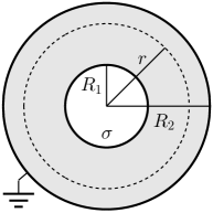
(a)

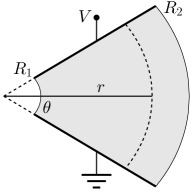
(b)

Figure 1: Model systems. (a) Cross section through the diameter of concentric cylinders or spheres with surface charge density $\sigma$. Distance $r$ is measured from the center of the cylinder/sphere, and the boundaries are located at $R_{1}$ and $R_{2}$. (b) Cross section of two flat-plate electrodes with an opening angle $\theta$ and potential difference $V$. Distance $r$ is measured from the “intersection” of the two plates, and the boundaries $R_{1}$ and $R_{2}$ mark the ends of the plates. Shading shows the space occupied by the liquid mixture.

In this manuscript we mainly present results for cylindrical geometry. This geometry intrinsically presents a mathematically unsavory dependence of $f_{\mathrm{e}}$ on $\phi$ (via $\varepsilon(\phi)$), and therefore creates more complicated solutions than, for example, in the wedge. Also, the difference in equational form between the cylinder and sphere does not present new information for discussion. The methods presented here can easily be adapted to both wedge and sphere geometries.

As will become evident, the precise surface charge density (surface potential) necessary to induce a transition depends on experimental parameters like the size and relative concentration of the liquid molecules, size of the charged material, temperature, etc. We consider a wide range of surface charges $\sigma$, from approximately zero up to $2\times 10^{-3}\,\mathrm{C/m^{2}}$ (equivalent to $1.25\times 10^{-2}~{}e/\mathrm{nm}^{2}$). For comparison, colloidal particles immersed in the non-polar phase of an inverse-micelle liquid have been measured to have large surface potentials, with an estimate of $200$ to $900e$ charges Hsu2005 . This amount of charge on a colloid could induce phase separation in a binary mixture if its composition is close enough to the demixing curve. The demixed liquid layer surrounding the colloid is predicted to be several tens to hundreds of nanometers thick, thereby altering the local environment of the colloid in an otherwise mixed liquid suspension. Of course, having the ability to externally apply a field, for example via an electrode, can be useful in some applications.

II Phase Diagram without an Electric Field

We briefly discuss some features of the mixing-demixing phase diagram in the absence of electric fields that are essential in the derivations below. A “double well” function (for example eq. 2 when $T<T_{c}$) possesses two local minima, one local maximum, and two inflection points located between the maximum and each minimum.

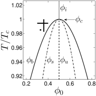
(a)

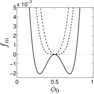
(b)

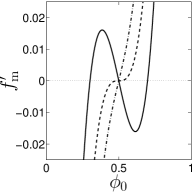
(c)

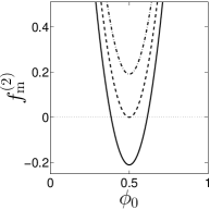
(d)

Figure 2: Free energy of mixing $f_{\mathrm{m}}$. (a) Phase diagram in the $\phi_{0}-T$ plane showing the zero-field binodal curve ($\phi_{b}$, thick solid line), spinodal curve ($\phi_{s}$, dash-dotted line), unstable solution ($\phi_{u}$, dashed line), critical point $\phi_{c}$, and the minimum of $f_{\mathrm{m}}$ above $T_{c}$ ($\phi_{i}$, thin solid line). Symbol marks the location of data in Fig. 4(a), while horizontal and vertical bars mark the location of data in Figs. 4(c) and 4(d), respectively. (b-d) Plots of $f_{\mathrm{m}}$ and it’s derivatives with respect to $\phi$ versus $\phi_{0}$ for $T$ less than (solid line), equal to (dashed line), and greater than (dash-dotted line) $T_{c}$. In this and in all other figures $T_{c}=298\,\mathrm{K}$, $\varepsilon_{A}=5$, $\varepsilon_{B}=3$, $R_{1}=1\,\mu\mathrm{m}$ and $Nv=1\times 10^{-26}\,\mathrm{m}^{3}$.

To ascertain the minimum of $f_{\rm m}$ at constant $T$, we find the solution to $f_{\rm m}^{\prime}=0$, Fig. 2(c), that also satisfies $f_{\rm m}^{(2)}>0$, Fig. 2(d), where the derivatives are taken with respect to $\phi_{0}$. The two solutions $\phi_{b}(T)=1/2\pm\sqrt{3(T_{c}-T)/4T)}$ for each $T<T_{c}$ create the binodal curve, thick solid line in Fig. 2(a). Fluids demix if the initial conditions $(\phi_{0},T)$ are under the binodal curve, and mix if they are above this curve. There in fact exists a third solution to $f_{\mathrm{m}}^{\prime}=0$, Fig. 2(c)—the local maximum at concentration $\phi_{u}(T)$, dashed line in Fig. 2(a). Even though this solution is physically unstable [$f_{\rm m}^{(2)}(\phi_{u})<0$, Fig. 2(d)], it will be useful in subsequent sections. If the local minima satisfy $f_{\rm m}^{(2)}>0$ and the local maximum satisfies $f_{\rm m}^{(2)}<0$, then there must exist inflection points between the extrema that satisfy $f_{\rm m}^{(2)}=0$, Fig. 2(d). These solutions $\phi_{s}(T)=1/2\pm\sqrt{(T_{c}-T)/4T}$ for each $T<T_{c}$ create the spinodal line, dash-dotted line in Fig. 2(a), and describe liquid behavior dynamically. If the initial point $(\phi_{0},T)$ is located below the spinodal curve, then the liquids demix spontaneously. If, however, $\phi_{0}$ exists between $\phi_{b}$ and $\phi_{s}$, then the liquid can be “stuck” in a local minimum, resulting in a metastable mixed state.

At the critical point $(\phi_{c},T_{c})$ the shape of $f_{\rm m}$ changes from having a single to double minima. As $T$ increases to $T_{c}$, the two minima $\phi_{b}$, the two inflection points $\phi_{s}$, and maximum $\phi_{u}$ converge and convert into a single minimum $\phi_{c}$. To meet these requirements the critical point must satisfy $f^{\prime}_{\rm m}=f^{(2)}_{\rm m}=f^{(3)}_{\rm m}=0$ and $f^{(4)}_{\rm m}>0$. Figures 2(c) and 2(d) display two of the four requirements. Finally, the light solid line in Fig. 2(a) shows the single solution $\phi_{i}(T)$ to $f_{\rm m}^{\prime}=0$ above the critical point.

III Defining Phase Separation

Nonuniform electric fields impose a nonuniform “pull” on the liquid mixture, manifesting as an $r$-dependent total free energy density $f(\phi,r)=f_{\mathrm{m}}(\phi)+f_{\mathrm{e}}(\phi,r)-\phi\mu$. The behavior of $f$ can be conceptualized as a competition between mixing and electrostatic energies. As $r\to\infty$, the electric field is weak, $f_{\mathrm{e}}\to 0$, and $f\approx f_{\mathrm{m}}-\phi\mu$ governs liquid behavior. The solid line in Fig. 3(a) shows a typical example of $f(\phi,r)$ at a large value of $r$ using $\phi_{0}=0.33$, $T/T_{c}=0.98$, and $\sigma=1.428\times 10^{-3}\,\mathrm{C/m^{2}}$ in an open cylinder system. The minimum of $f(\phi,r)$, marked by a symbol, gives the value of $\phi(r)$ as $r\to\infty$, which in this case is $0.33$. At the other distance extreme, $r=R_{1}$, the electric field is the strongest, and the dashed line in Fig. 3(a) shows the resulting $f(\phi,r)$. Note the dramatic difference in the value of $\phi(r)$ when the value of $r$ is small ($R_{1}$) versus large.

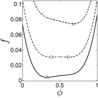
(a)

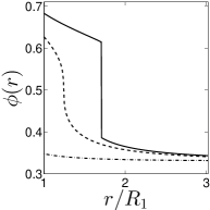
(b)

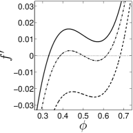
(c)

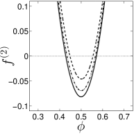
(d)

Figure 3: Free energy density $f(\phi,r)$ for an open cylinder system. (a,c,d) $f$, $f^{\prime}$, and $f^{(2)}$, respectively, versus $\phi$ at distance $r=R_{1}$ (dashed line), $r_{i}$ (dash-doted line), and a large value (solid line) for $\phi_{0}=0.33$, $T/T_{c}=0.98$, and $\sigma=1.428\times 10^{-3}\,\mathrm{C/m^{2}}$. Symbols in (a) mark minima for each curve. (b) $\phi(r)$ versus normalized distance $r$. Solid line is data from (a). Dash-dotted line has same $\phi_{0}$ and $T$ as (a) but with smaller $\sigma=0.540\times 10^{-3}\,\mathrm{C/m^{2}}$. Dashed line has same $\phi_{0}$ and $\sigma$ as (a) but with larger $T/T_{c}=0.995$.

By finding the minimum of $f$ for all values of $r$, it is possible to construct the full concentration profile $\phi(r)$, where the solid line in Fig. 3(b) corresponds to the data from Fig. 3(a). Whether or not a phase transition occurs in the equilibrium solution resides in how the minimized $f(\phi,r)$ changes as $r$ varies between the two distance extremes. Specifically, if there exists an $r=r_{i}$ where $R_{1}\leq r_{i}\leq R_{2}$ and $f(\phi,r_{i})$ contains two minima [see dash-dotted line in Fig. 3(a)], then $r_{i}$ is an interface between the two liquids. Figure 3(b) illustrates how the two minima in $f(\phi,r_{i})$ translate into a discontinuity at $\phi(r_{i})$, thereby creating a distinct boundary between the two phases.

A closer inspection of $f(\phi,r)$ at $r=r_{i}$ reveals important mathematical features similar to those in $f_{\rm m}(\phi)$ discussed in the previous section. The similarity is not surprising, since $f_{\mathrm{m}}(\phi)$ is a component of $f(\phi,r)$. The dash-dotted lines in Figs. 3(a), 3(c), and 3(d) show that $f(\phi,r_{i})$ possesses two local minima we call $\phi_{iH}$ and $\phi_{iL}$, one local maximum $\phi_{u}$, and two inflection points we call $\phi_{sH}$ and $\phi_{sL}$. In addition, $f(\phi,r_{i})$ can have critical behavior. We will demonstrate that all these features at $r_{i}$ behave analogously to those in Fig. 2(a) and show how to use this information to construct the mixing-demixing phase diagram with an electric field.

IV Composition Profiles $\phi(r)$ and Location of the Interface

Not all applied fields induce liquid demixing, and based on our definition of a phase transition, there are two possible causes. First, $r_{i}$ exists in “virtual” ($r_{i}<R_{1}$ or $r_{i}>R_{2}$) rather than “real” space, dash-dotted line in Fig. 3(b). Second, $f$ contains a single minimum for all $r$, including $r_{i}$, dashed line in Fig. 3(b).

We begin with the first cause. For a constant $\phi_{0}$ and $T$, Fig. 3(b) shows that certain values of $\sigma$ induce a transition, whereas others do not. In fact, there exists a transition $\sigma_{t}$ that marks the lowest $\sigma$ necessary for liquid-liquid separation. Figure 4(a) also shows how increasing $\sigma$ moves the interface $r_{i}$ to larger $r$, using an open cylinder system as an example. Noting that mathematical solutions exist for all $r$ (including those distances in non-physical space), the vertical dashed line in Fig. 4(a) at $r=R_{1}$ marks the surface of the cylinder. To the right of this line is real (physical) space, while to the left is the virtual space inside the electrode (or not between the plates as defined in Fig. 1(b) for wedge geometries). This observation inspires an alternative definition: the surface charge density $\sigma_{t}$ is the $\sigma$ that places $r_{i}$ exactly at $R_{1}$. We stress that profiles $\phi(r)$ at constant $\phi_{0}$ and $T$ in open systems with varying values of $\sigma$ all collapse to a single curve when plotted versus a scaled distance $(r-r_{i})/(\sigma R_{1})$, Fig. 4(b).

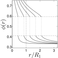
(a)

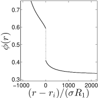
(b)

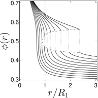
(c)

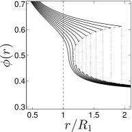
(d)

Figure 4: Variation of concentration profiles $\phi(r)$ for an open cylinder system. (a) $\phi(r)$ versus normalized distance $r$ for constant $\phi_{0}=0.33$, $T/T_{c}=0.985$, and varying $\sigma=0.4\times 10^{-3}$ to $2.0\times 10^{-3}\,\mathrm{C/m^{2}}$ in $0.4\times 10^{-3}$ increments (lines, left to right). (b) Data in (a) collapses when plotted versus a rescaled distance $(r-r_{i})/(\sigma R_{1})$. (c) $\phi(r)$ versus $r$ for constant $T/T_{c}\approx 0.994$, $\sigma=1\times 10^{-3}\,\mathrm{C/m^{2}}$, and varying $\phi=0.3$ to $0.4$ in $0.01$ increments (lines, left to right). (d) $\phi(r)$ versus $r$ for constant $\phi=0.36$, $\sigma=1\times 10^{-3}\,\mathrm{C/m^{2}}$, and varying $T/T_{c}\approx 0.982$ to $1$ in $0.0016$ increments (lines, right to left).

Varying $\phi_{0}$ (holding $T$ and $\sigma$ constant) and $T$ (holding $\phi_{0}$ and $\sigma$ constant) reveals the second cause for no phase separation, illustrated in Fig. 4(c) and 4(d), respectively. In these cases, both the interface location $r_{i}$ and the size of the discontinuity change. Importantly, the discontinuity can even vanish, as the high and low concentrations $\phi_{iH}$ and $\phi_{iL}$ at the interface merge to the same value at certain $\phi_{0}$ or $T$. Notice the remarkable similarity between the behavior of the discontinuity at $r_{i}$, dash-dotted lines in Figs. 4(c) and 4(d), and the binodal curve, Fig. 2(a).

The location of the interface, once it exists, is controlled by $\phi_{0}$, $T$, $\sigma$ and $R_{2}$. In general, $r_{i}$ increases with increasing $\sigma$ [Fig. 4(a) and 5(a)], increasing $\phi_{0}$ [Fig. 4(c) and 5(b)], decreasing $T$ [Fig. 4(d) and 5(c)], and increasing $R_{2}$ [discussed in Sect. VII, Fig. 8(b)).

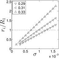
(a)

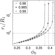
(b)

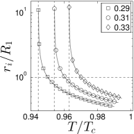
(c)

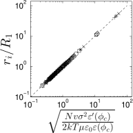
(d)

Figure 5: Controlling the location of the interface $r_{i}$ for an open cylinder system. (a) Normalized $r_{i}$ versus $\sigma$ [$\mathrm{C/m^{2}}$] for various values of $\phi_{0}$ where $T/T_{c}=0.975$. (b) Normalized $r_{i}$ versus $\phi_{0}$ for various values of $T/T_{c}$ where $\sigma\approx 5.4\times 10^{-4}\,\mathrm{C/m^{2}}$. (c) Normalized $r_{i}$ versus $T/T_{c}$ for various $\phi_{0}$ where $\sigma\approx 5.4\times 10^{-4}\,\mathrm{C/m^{2}}$. (d) Collapse of all data from (a-c) when $r_{i}$ is plotted against eq. 10. In (b,c), vertical dashed lines mark the binodal for the given values of $\phi_{0}$ and $T$.

Besides solving the full $\phi(r)$ profile, a quicker method for determining the location of the interface $r_{i}$ consists of solving these three equations Samin2009 ; Samin2011

$$f^{\prime}_{\mathrm{m}}(\phi_{iH})-f^{\prime}_{\mathrm{e}}(\phi_{iH},r_{i})-\mu=0$$

$$f^{\prime}_{\mathrm{m}}(\phi_{iL})-f^{\prime}_{\mathrm{e}}(\phi_{iL},r_{i})-\mu=0$$

$$f_{\mathrm{m}}(\phi_{iH})\pm f_{\mathrm{e}}(\phi_{iH},r_{i})-\phi_{iH}\mu=$$

$$f_{\mathrm{m}}(\phi_{iL})\pm f_{\mathrm{e}}(\phi_{iL},r_{i})-\phi_{iL}\mu$$ (8)

for three unknowns: $r_{i}$ and the high and low concentrations $\phi_{iH}$ and $\phi_{iL}$, respectively, at $r_{i}$. The plus (minus) sign in the third equation is for constant charge (potential) boundary conditions. The first two equations find extrema points and are simply eq. 6 or 7, depending on system geometry. The third equation ensures that the free energy for the high concentration $\phi_{iH}$ is as favorable as the low concentration $\phi_{iL}$.

An even simpler method for finding $r_{i}$ consists in recalling that there exists a third solution to $f^{\prime}$—the local maxima $\phi_{u}$, Fig. 3(c). For cylindrical ($n=1$) and spherical ($n=2$) geometries, the explicit equation for $f^{\prime}=0$ is

$$0 = 4\left(1-\frac{T_{c}}{T}\right)\left(\phi_{u}-\phi_{c}\right)+\frac{16}{3}\left(\phi_{u}-\phi_{c}\right)^{3}$$ (9)

$$-\frac{Nv}{2kT\varepsilon_{0}}\left(\frac{\sigma R_{1}^{n}}{r_{i}^{n}}\right)^{2}\frac{\varepsilon^{\prime}(\phi_{u})}{\varepsilon(\phi_{u})^{2}}-\mu$$

If $\phi_{u}$ is known, then $r_{i}$ can, in principle, be deduced from experimental parameters ($\phi_{0}$, $T$, etc.). For now, we will borrow ideas from the binodal curve and make the assumption $\phi_{u}=\phi_{c}=0.5$, but will see later that $\phi_{u}$ indeed approximately equals $\phi_{c}$ under many conditions. Rearranging eq. 9, we now have the useful relation

$$\left(\frac{\sigma R_{1}^{n}}{r_{i}^{n}}\right)^{2}=-\mu\frac{2kT\varepsilon_{0}}{Nv}\frac{\varepsilon(\phi_{c})^{2}}{\varepsilon^{\prime}(\phi_{c})}$$ (10)

In open systems, this equation is further simplified by substituting $\mu=\mu_{0}(\phi_{0})=f^{\prime}_{\mathrm{m}}(\phi_{0},T)$. The lines in Figs. 5(a), 5(b), and 5(c) use eq. 10 to solve $r_{i}$ in an open cylinder system, and reveal an excellent agreement to the solutions from eqs. 8 (symbols). Figure 5(d) combines all data from Figs. 5(a), 5(b), and 5(c), revealing that the agreement spans many orders of magnitude.

The analogous equation for finding $r_{i}$ in a wedge geometry is

$$\left(\frac{V}{\theta r_{i}}\right)^{2}=-\frac{2kT\mu}{Nv\varepsilon_{0}\varepsilon^{\prime}(\phi_{c})}$$ (11)

V Stability Diagram and Electrostatic Binodal

If an electric field can cause phase separation in a region of $\phi_{0}-T$ space above the binodal curve, a natural question arises: what is the new stability diagram for a particular value of surface charge density $\sigma$? This can be constructed by holding $\sigma$ constant and probing $\phi_{0}-T$ space for liquid-liquid demixing. Since the electric field breaks the symmetry of the free energy with respect to composition ($\phi_{0}\to 1-\phi_{0}$), the stability diagram is asymmetric with respect to $\phi_{0}-\phi_{c}$. Figure 6(a) compares a typical stability curve for an open cylindrical system, solid line, to the binodal curve, dashed line. Clearly, nonuniform fields can produce large changes to the phase diagram.

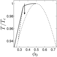
(a)

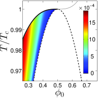
(b)

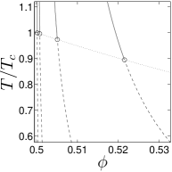
(c)

(d)

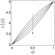
(e)

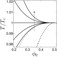
(f)

Figure 6: Electrostatic binodal in open systems. (a) Stability diagram (solid line) and electrostatic spinodal (dash-dotted line) in $\phi_{0}-T$ plane for $\sigma=1\times 10^{-3}\,\mathrm{C/m^{2}}$. Dashed line is binodal curve. Path of arrow marks location of data in Fig. 4(d). (b) Overlay of many stability diagrams, where color indicates transition $\sigma_{t}$ [$\mathrm{C/m^{2}}$]. Solid line is electrostatic binodal from eq. 14, where thick and thin marks show where values of $\sigma_{t}=\sigma_{K}$ are real and imaginary, respectively. (c) Solutions $\phi_{i}$ (solid lines), $\phi_{iC}$ (symbols), and $\phi_{u}$ (dashed lines) to $f^{(3)}=0$ versus $T$ where $\sigma=0.5\times 10^{-3}$, $1\times 10^{-3}$, $2.5\times 10^{-3}$, and $5\times 10^{-3}\,\mathrm{C/m^{2}}$ (lines, left to right). Dotted curve shows $\phi_{iC}$ for all $\sigma$. (d) Critical $\sigma_{K}$ [$\mathrm{C/m^{2}}$] along electrostatic binodal versus $T_{K}$. (e) Quadratic forms of $\varepsilon(\phi)$ versus $\phi$, where the second derivative $\varepsilon^{(2)}(\phi)=-2$, $-1$, $0$, $1$, and $2$ (arrow). (f) Solid lines show electrostatic binodal for an open wedge system using $\varepsilon^{(2)}(\phi)$ from (e) (arrow). Dash-dotted line shows electrostatic binodal using Flory-Huggins theory for $f_{\mathrm{m}}$ and $\varepsilon^{(2)}(\phi)=-2$. Dashed line is binodal curve.

Figure 6(b) shows the superposition of stability diagrams from a wide range of $\sigma$ in an open cylindrical system, where the color indicates the transition $\sigma_{t}$ for each point $(\phi_{0},T)$. (Points beneath the binodal curve are omitted since phase separation occurs there without an electric field.) Figure 6(b) clearly illustrates two distinct regions in the $\phi_{0}-T$ plane. In the “demixed” region, there exists a $\sigma_{t}$ for each ($\phi_{0}$,$T$) such that any $\sigma\geq\sigma_{t}$ results in liquid demixing. In the “mixed” region, there does not exist any $\sigma$ that results in liquid demixing. Notice how the mixed region extends well below $T_{c}$, indicating that simply setting $T<T_{c}$ is not sufficient for producing a phase transition with an electric field. We will call the curve that divides these two regions the “electrostatic binodal”.

To derive the electrostatic binodal, we draw inspiration from the “regular” binodal curve. The convergence of the interface concentrations $\phi_{iH}$ and $\phi_{iL}$ in Figs. 4(c) and 4(d) suggest the existence of a critical point at $r_{i}$. If there exists a critical point at $r_{i}$, then the two minima $\phi_{iH}$ and $\phi_{iL}$, the local maximum $\phi_{u}$, and the two inflection points $\phi_{sH}$ and $\phi_{sL}$ converge to a single point $\phi_{iC}$, resulting in $f^{\prime}(r_{i})=f^{(2)}(r_{i})=f^{(3)}(r_{i})=0$ and $f^{(4)}(r_{i})>0$. We call the coordinates in the $\phi_{0}-T$ plane that produce a critical point at $r_{i}$ the critical $\phi_{K}$ and critical $T_{K}$.

We now show one method for finding $\phi_{K}$ and $T_{K}$, using an open cylinder system as an example and begin with $f^{(2)}=0$:

$$2\left(1-\frac{T_{c}}{T_{K}}\right)+8\left(\phi_{iC}-\phi_{c}\right)^{2}+$$

$$\frac{Nv}{2kT_{K}\varepsilon_{0}}\frac{[\varepsilon^{\prime}(\phi_{iC})]^{2}}{\varepsilon(\phi_{iC})^{3}}\left(\frac{\sigma R_{1}}{r_{i}}\right)^{2} = 0$$ (12)

The derivation of eq. 10 depends on finding $\phi$ that satisfies $f^{\prime}=0$, but does not specify $\phi$ as a local maximum or minimum. In particular, $\phi_{iC}$ also satisfies eq. 10. We therefore substitute eq. 10 for $(\sigma R_{1}/r_{i})^{2}$ into eq. 12, use $\mu=\mu_{0}(\phi_{K})=f^{\prime}_{\mathrm{m}}(\phi_{K},T_{K})$ for an open system, and rearrange to obtain

$$\frac{T_{K}}{T_{c}} = \left[\frac{4\left(\phi_{iC}-\phi_{c}\right)^{2}-\frac{8}{3}\left(\phi_{K}-\phi_{c}\right)^{3}\frac{\varepsilon^{\prime}(\phi_{iC})}{\varepsilon(\phi_{iC})}}{1-2\left(\phi_{K}-\phi_{c}\right)\frac{\varepsilon^{\prime}(\phi_{iC})}{\varepsilon(\phi_{iC})}}+1\right]^{-1}$$ (13)

$${\rm open~{}cylinder}$$

Notice that as $\varepsilon^{\prime}\to 0$, we recover the solution to $f_{\mathrm{m}}^{(2)}=0$, and $T_{K}\to T_{c}$ when $\phi_{i}$ equals the critical composition $\phi_{c}$.

Proceeding, $\phi_{iC}$ must also satisfy $f^{(3)}=0$ at $r_{i}$. Figure 6(c) shows the solutions to $f^{(3)}=0$ for a wide range of $T$, where the curves from left to right are low to high $\sigma$. The values of $\phi_{i}$ (solid lines), $\phi_{iC}$ (symbols), and $\phi_{u}$ (dashed lines) form a continuous variation with $T$, Fig. 6(c), analogous to $\phi_{i}$, $\phi_{c}$, and $\phi_{u}$ with $f_{\mathrm{m}}$, Fig. 2(a). Since $\phi_{iC}\approx\phi_{c}$, Fig. 6(c), we can simplify eq. 13 to obtain the expression for the electrostatic binodal in an open cylinder system

$$\frac{T_{K}}{T_{c}}\approx\left[\frac{-\frac{8}{3}\left(\phi_{K}-\phi_{c}\right)^{3}\frac{\varepsilon^{\prime}(\phi_{c})}{\varepsilon(\phi_{c})}}{1-2\left(\phi_{K}-\phi_{c}\right)\frac{\varepsilon^{\prime}(\phi_{c})}{\varepsilon(\phi_{c})}}+1\right]^{-1}~{}~{}~{}~{}{\rm open~{}cylinder}$$ (14)

Interestingly, this equation only depends on $\phi_{K}$ and the functional form of $\varepsilon(\phi)$, but is independent of $\sigma$ and $r_{i}$. This finding is a consequence of the self-similarity of solutions in open systems for a constant $\phi_{0}$ and $T$, described in Sect. IV and shown in Fig. 4(b). Moreover, the geometry difference between cylinders and spheres does not influence the electrostatic binodal. Equation 14 is, in fact, the same equation for the electrostatic binodal in an open sphere system, using the same assumptions.

The thick solid line in Fig. 6(b) shows the results from eq. 14, as it accurately divides the $\phi_{0}-T$ plane into mixed and demixed regions. With each point $(\phi_{K},T_{K})$, there is an associated critical $\sigma_{K}$: the $\sigma$ that places $r_{i}$ exactly at $R_{1}$. It’s important to recognize that $\sigma_{K}$ is not constant along the electrostatic binodal—$\sigma_{K}$ is $0$ at $T_{K}=T_{c}$ and increases as $T_{K}$, Fig. 6(d), and/or $\phi_{K}$ decrease. Figure 6(d) compares $\sigma_{K}$ from calculations (symbols) versus $\sigma_{K}$ derived from eq. 10 using $\phi_{K}$, $T_{K}$, and $r_{i}=R_{1}$ (line). Equation 14 predicts that the electrostatic binodal also exists for $\phi_{0}>\phi_{c}$, thin solid line in Fig. 6(b); however, the associated values of $\sigma_{K}$ are imaginary and not possible in real physical systems.

The electrostatic binodal is a line of critical points, or simply a “critical line”. This finding explains some curious observations found previously Samin2009 : If $\phi_{0}$ and/or $T$ is changed such that the stability diagram for a constant $\sigma$ is crossed on the boundary between the kink and $(\phi_{c},T_{c})$, for example the arrow in Fig. 6(a), then $r_{i}$ emerges at some distance greater than $R_{1}$, Fig. 4(d). The kink marks $(\phi_{K},T_{K},\sigma=\sigma_{K})$. The boundary of the stability diagram to the right of the kink is exactly the electrostatic binodal. On this boundary, $\sigma$ is now larger than $\sigma_{K}$. In other words, $\sigma$ is no longer the minimum surface charge that induces the transition; therefore, $r_{i}$ necessarily emerges at some distance greater than $R_{1}$.

The open wedge system produces analogous results; however, we will use the simplicity of the equations in this geometry to demonstrate the effects of quadratic $\varepsilon(\phi)$ relations, Fig. 6(e). Following the same reasoning as for an open cylinder system, we find the electrostatic binodal for an open wedge

$$\frac{T_{K}}{T_{c}} = \left[\frac{\frac{4}{3}\left(\phi_{K}-\phi_{c}\right)^{3}\frac{\varepsilon^{(2)}(\phi_{c})}{\varepsilon^{\prime}(\phi_{c})}}{1+\left(\phi_{K}-\phi_{c}\right)\frac{\varepsilon^{(2)}(\phi_{c})}{\varepsilon^{\prime}(\phi_{c})}}+1\right]^{-1}$$ (15)

$${\rm open~{}wedge}$$

We add that $\phi_{i}$, $\phi_{iC}$, and $\phi_{u}$ exactly equal $\phi_{c}$ if $\varepsilon^{(2)}(\phi)$ and higher derivatives vanish. Notice the similarity between eqs. 14 and 15, where the main difference is that higher derivatives of $\varepsilon(\phi)$ control the electrostatic binodal in the wedge geometry. Figure 6(f) shows how the electrostatic binodal for the wedge curves downwards to upwards as $\varepsilon^{(2)}(\phi_{c})$ changes from negative to positive. And if $\varepsilon^{(2)}(\phi_{c})=0$, then $T_{K}$ for the electrostatic binodal simply equals $T_{c}$ for all $\phi_{K}$. By comparing Fig. 6(e) to the results in Fig. 6(f), it is evident that small amounts of curvature in $\varepsilon(\phi)$ can create large changes in the electrostatic binodal, in agreement with previous findings Samin2009 .

We briefly discuss an alternate derivation presented in Ref. Samin2009 to emphasize that we have not exhausted all possible relations between parameters. Beginning with $f^{(2)}=f^{(3)}=0$ for $r_{i}=R_{1}$ and $\varepsilon^{(3)}(\phi)=0$ in the wedge geometry, we obtain

$$\frac{T_{K}}{T_{c}}=1+\frac{Nv\varepsilon_{0}\varepsilon^{(2)}(\phi)}{8kT_{c}}\left(\frac{V_{K}}{\theta R_{1}}\right)^{2}$$ (16)

Interestingly, using the Flory-Huggins approximation for $f_{\mathrm{m}}$ results in exactly the same relation, eq. 16, as the Landau approximation. The differences between the two approximations instead arise when determining $\phi_{K}$, where the biggest discrepancies occur, as expected, for values of $\phi_{K}$ that are far from $\phi_{c}$, Fig. 6(f).

VI Electrostatic Spinodal

We now turn the discussion to possible metastable states, recalling the meaning of the spinodal curve in the mean-field theory  Binder2009 . Earlier in the manuscript, we rationalized the existence of inflection points $\phi_{s}$ at $r_{i}$ through the presence of a maximum $\phi_{u}$ and minima $\phi_{iH}$, $\phi_{iL}$. Both high and low values $\phi_{sH}$, $\phi_{sL}$ satisfy $f^{(2)}=0$ and exist at all interfaces. Figure 7(a), for example, explicitly shows the mathematical features [$\phi_{iH}$, $\phi_{iL}$ (solid line), $\phi_{sH}$, $\phi_{sL}$ (dash-dotted line), $\phi_{u}$ (dashed line), and critical point] occurring at $r_{i}$ with changing $T$ in an open cylinder system. For comparison, the dotted lines display the behavior of the binodal points $\phi_{b}$ with $T$.

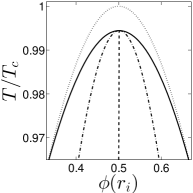
(a)

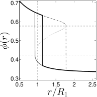
(b)

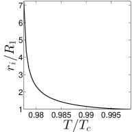
(c)

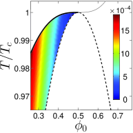
(d)

Figure 7: Electrostatic spinodal for an open cylinder system. (a) Behavior of $\phi(r_{i})$ with $T$, showing $\phi_{iH}$, $\phi_{iL}$ (solid line), $\phi_{sH}$, $\phi_{sL}$ (dash-dotted line), and $\phi_{u}$ (dashed line). Lines converge at the critical point $\phi_{iC}$. In all data, $\phi_{0}=0.33$ and $\sigma\approx 2.09\times 10^{-3}\,\mathrm{C/m^{2}}$. Dotted lines show $\phi_{b}$. (b) All $\phi(r)$ solutions to $f^{\prime}=0$ versus normalized $r$. Thin solid, dash-dotted, and dotted lines show lower, upper, and unstable solutions, respectively, for $\phi_{0}=0.33$, $T/T_{c}=0.975$, and $\sigma=8\times 10^{-4}\,\mathrm{C/m^{2}}$. Thick line shows the solution that minimizes $f$. Horizontal dashed lines show $\phi_{sL}$ and $\phi_{sH}$. (c) Location of the interface $r_{i}$ versus normalized $T$ along the spinodal line in Fig. 6(a) for $\sigma=1\times 10^{-3}\,\mathrm{C/m^{2}}$. (d) Overlay of electrostatic spinodals for many $\sigma$ (color, [$\mathrm{C/m^{2}}$]).

Despite the ubiquitous presence of $\phi_{sH}$ and $\phi_{sL}$, only $\phi_{sL}$ carries physical meaning in open systems, and only in a limited region of the stability diagram. To see how this occurs, we return to the solutions of $f^{\prime}=0$. Thus far, we focused on $r_{i}$, the location of the interface for the minimized $f$; however, there can be many $r$ that posses the same mathematical features. Figure 7(b) shows all possible solutions to $f^{\prime}=0$, where the thin solid, dash-dotted, and dotted lines are the “lower”, “upper”, and “unstable” solutions, respectively. The heavy solid line depicts the solution that actually minimizes $f$, and the two dashed lines denote $\phi_{sH}$ and $\phi_{sL}$ found at $r_{i}$.

We start from a homogeneous mixture at composition $\phi_{0}$ and perform the thought experiment of turning on an electric field. Considering diffusive liquid movement in the absence of other factors (ex. liquid convection, noise), this experimental setup implies that the profile $\phi(r)$ initially develops along the free energy “well” created by the lower solution. If the electric field can sufficiently “pull” the higher dielectric material such that there is at least one distance $r$ where $\phi(r)\geq\phi_{sL}$, then the liquid can escape the metastable (mixed) state at the local free energy minimum to find the global minimum (demixed). We call $r_{s}$ the distance where $\phi(r_{s})=\phi_{sL}$ and find $r_{s}$ by solving $f^{\prime}=0$ at $\phi_{sL}$. For a cylindrical geometry we have

$$\frac{r_{s}}{R_{1}}=\sqrt{\frac{Nv}{2kT\varepsilon_{0}}\left[\frac{\sigma^{2}}{f^{\prime}_{m}(\phi_{sL})-\mu}\right]\frac{\varepsilon^{\prime}(\phi_{sL})}{\varepsilon(\phi_{sL})^{2}}}$$ (17)

Knowing that the highest value of $\phi(r)$ occurs closest to the electrode at $R_{1}$, we seek the conditions where $r_{s}=R_{1}$. These conditions, therefore, mark the electrostatic spinodal: If $r_{s}\geq R_{1}$ at a particular $(\phi_{0},T,\sigma)$, then demixing occurs spontaneously. If $r_{s}<R_{1}$ at a particular $(\phi_{0},T,\sigma)$, for example Fig. 7(b), then the liquids can be metastabaly mixed. The long time solution for dynamics in these cases therefore resides along the thin solid curve, Fig. 7(b).

Figure 6(a) shows the location of the electrostatic spinodal for a particular value of $\sigma$. The curve begins at the critical point $(\phi_{K},T_{K})$ and travels down, on the right side of the stability diagram boundary. Similar to the “regular” spinodal curve, demixing occurs spontaneously (non-spontaneously) for $(\phi_{0},T)$ to the right (left) of the electrostatic spinodal. Since the electrostatic spinodal cuts inside the stability diagram, the location of the interface $r_{i}$ emerges at distances greater than $R_{1}$, with $r_{i}=R_{1}$ only at $(\phi_{K},T_{K})$. Figure 7(c) displays the behavior of $r_{i}$ along the spinodal in Fig. 6(a). Finally, the electrostatic spinodal exists for all $\sigma$. Figure 7(d) shows the superposition of the electrostatic spinodal curves, where the color indicates the associated $\sigma$.

VII Closed Systems

Up until now, we focused on liquid behavior in open systems, where we considered the location of the second boundary as $R_{2}\to\infty$. A closed system with a finite $R_{2}$ markedly alters the phase diagram Samin2009 ; however, we will show that these alterations naturally arise from the solutions of open systems.

We begin as previously, with variations in the concentration profiles $\phi(r)$, and identify interesting changes with two parameters, $\sigma$ and $R_{2}$. Both Figs. 8(a) and 8(b) clearly reveal that the discontinuity at the interface decreases and vanishes with increasing $\sigma$ and decreasing $R_{2}$, respectively, in closed cylinder systems. Intriguingly, the profiles in Fig. 8(a) stand in sharp contrast to the self-similar solutions found in open systems, Figs. 4(a) and 4(b). Closer inspection of Fig. 8(a) also reveals that the parabolic-like shape in the discontinuity with various $\sigma$ opens to the left, rather than to the right as in Figs. 4(c), 4(d), and 8(b). An important consequence is that for closed systems there are two transition surface charge densities $\sigma_{t}$: the first $\sigma_{t1}$ is the $\sigma$ that places $r_{i}$ exactly at $R_{1}$, while the second $\sigma_{t2}$ is the $\sigma$ where the interface discontinuity vanishes. Therefore, the interface between the liquids in closed systems only exists when $\sigma$ satisfies $\sigma_{t1}\leq\sigma\leq\sigma_{t2}$, shaded region in Fig. 8(c).

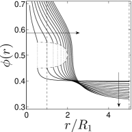
(a)

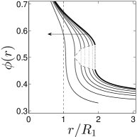
(b)

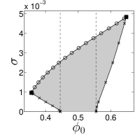
(c)

Figure 8: Variation of concentration profiles $\phi(r)$ in a closed cylinder system. (a) $\phi(r)$ versus a normalized distance $r$ for a constant $\phi_{0}=0.4$, $T/T_{c}\approx 0.996$, $R_{2}/R_{1}=5$ and varying $\sigma=0.25\times 10^{-3}$ to $3\times 10^{-3}\,\mathrm{C/m^{2}}$ in $0.25\times 10^{-3}$ increments (arrows). (b) $\phi(r)$ versus a normalized distance $r$ for a constant $\phi_{0}=0.36$, $T/T_{c}\approx 0.995$, $\sigma=1.5\times 10^{-3}\,\mathrm{C/m^{2}}$ for an open system (thick line) and closed systems (thin lines) with decreasing $R_{2}/R_{1}=20$, $12$, $8$, $6$, $4$ to $2$ (arrow). (c) $\sigma_{t1}$ ($\times$), $\sigma_{t2}$ ($\circ$), and $\sigma_{K}$ (filled squares) versus $\phi_{0}$ for $T/T_{c}=0.996$ and $R_{2}/R_{1}=5$. Dashed lines show binodal $\phi_{b}$ at same $T$. Phase separation occurs in shaded region.

Material conservation drives all differences between closed and open systems, thus, the key to understanding these differences resides in understanding $\mu$. Recall that $\mu=\mu_{0}=f_{\mathrm{m}}^{\prime}(\phi_{0},T)$ in open systems, while $\mu$ is adjusted to account for material conservation in closed systems. Mathematically, the adjusted $\mu$ for a closed system at $(\phi_{0},T)$ exactly matches the $\mu_{0}$ for an open system with a different “effective” concentration $\phi_{E}$ in the bath. Consequently, the $\phi(r)$ profile between $R_{1}$ and $R_{2}$ at $(\phi_{0},T)$ in a closed system exactly matches the $\phi(r)$ profile at $(\phi_{E},T)$ in an open system. In other words, the behavior of a closed system maps onto that of an open system via $\phi_{E}$.

We can explain the variation of $\phi(r)$ with $\sigma$ in closed systems using this construct. Intuitively, the higher dielectric material is pulled closer to the electrode as the value of $\sigma$ increases. In order to conserve material in a closed system, $\phi(r)$ necessarily decreases near $R_{2}$, Fig. 8(a). This shift in liquid concentration translates as a decrease in $\phi_{E}$, hence increasing $\sigma$ in a closed system maps as increasing $\sigma$ and decreasing $\phi_{E}$ in an open system. Recall that the interface discontinuity becomes smaller with lower $\phi_{E}$ in an open cylinder system, Fig 4(c), and eventually vanishes when $\phi_{E}$ crosses the electrostatic binodal. The same principles apply to closed systems, where the second transition $\sigma_{t2}$ marks this crossing.

Now that we understand how experimental parameters change $\phi(r)$, we focus on how these changes affect the stability diagram. Figure 9(a) shows a typical stability diagram for a constant $\sigma=1\times 10^{-3}\,\mathrm{C/m^{2}}$ and $R_{2}/R_{1}=5$ in a closed cylinder system. One striking difference between open, Fig. 6(a), and closed, Fig. 9(a), systems is that liquid separation can now occur for $\phi_{0}>\phi_{c}$. Experimentally, this manifests as an interface emerging close to $R_{2}$, rather than $R_{1}$. A second more subtle difference is that the stability diagram for closed systems occupies a slightly smaller region of $\phi_{0}-T$ space for $\phi_{0}\leq\phi_{c}$ compared to open systems with the same $\sigma$. Finally, the upper boundary for the closed system stability curve travels below $T_{c}$ to exclude a portion of the binodal curve. Closed systems, therefore, provide the interesting possibility of an electric field mixing liquids that normally demix.

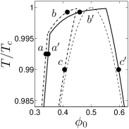
(a)

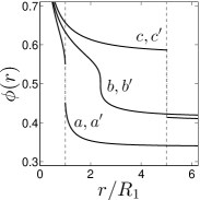
(b)

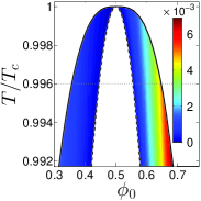
(c)

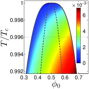
(d)

(e)

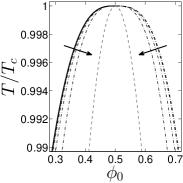
(f)

Figure 9: Electrostatic binodal in a closed cylinder system. (a) Stability curve (solid line) in $\phi_{0}-T$ space for a constant $\sigma=1\times 10^{-3}\,\mathrm{C/m^{2}}$ and $R_{2}/R_{1}=5$. Dash-dotted line shows the mapping of the stability diagram boundaries to an open system via $\phi_{E}$ (see text). Dashed line shows binodal curve. (b) $\phi(r)$ versus normalized $r$ for points marked by symbols in (a). Dashed lines mark the boundaries of the container. (c,d) Overlay of many stability diagrams, where color indicates transition $\sigma_{t1}$ and $\sigma_{t2}$ [$\mathrm{C/m^{2}}$], respectively. Dotted lines show location of data in Fig. 8(c). (e) Critical surface charge density $\sigma_{K}$ on the electrostatic binodal for $\phi_{K}\leq\phi_{c}$ (solid line) and $\phi_{K}\geq\phi_{c}$ (dash-dotted lines) for $R_{2}=20$, $10$, $5$, and $2.5\,\mu\mathrm{m}$ (arrow). (f) Electrostatic binodal for open (solid line) and closed (dash-dotted lines) systems for the same $R_{2}$ as (e). Curves are not symmetric around $\phi_{0}=0.5$. Dashed line shows binodal curve.

We can use the mapping construct to not only comprehend these changes but also to produce the stability diagram of closed system. Open systems link to closed systems via integration. Specifically, integrating $\phi(r)$ between $R_{1}$ and $R_{2}$ in an open system at $(\phi_{E},T)$ gives the corresponding $(\phi_{0},T)$ for the closed system. We begin with the left boundary of the stability diagram for an open system, label $a$ in Fig. 9(a), and integrate $\phi(r)$ between $R_{1}$ and $R_{2}$ to determine the location of the left boundary in a closed system, label $a^{\prime}$ in Fig. 9(a). The difference between $\phi_{E}$ and $\phi_{0}$ along this boundary is small. If we look at an example $\phi(r)$ profile, Fig. 9(b), we see that the interface location $r_{i}$ equals $R_{1}$ and that the electric field for $r>R_{1}$ produces only small variations in $\phi(r)$. Truncating the integration at $R_{2}$, therefore, only minimally alters the liquid concentration.

Next, we consider the upper boundary of the open system stability diagram, label $b$ in Fig. 9(a), and integrate from $R_{1}$ to $R_{2}$ to obtain the upper boundary for the closed system stability diagram, label $b^{\prime}$ in Fig. 9(a). Here, large differences between $\phi_{E}$ and $\phi_{0}$ can occur. This boundary for open systems is the electrostatic binodal. As previously described in Sect. V, $\sigma>\sigma_{K}$, which causes the location of the interface $r_{i}$ to emerge at distances greater than $R_{1}$. The inclusion of high dielectric material from $R_{1}$ to $r_{i}$ can substantially increase $\phi_{0}$ when integration stops at $R_{2}$.

The upper boundary of the stability diagram for a closed system ends when $r_{i}=R_{2}$. And to form the right boundary in a closed system, we must find the conditions where $\sigma$ places $r_{i}$ at $R_{2}$ in an open system. There are two methods by which to proceed. First, we present the simple straightforward approach. We use eq. 10 with $\sigma$, $r_{i}=R_{2}$, and various $T$ to determine the appropriate $\phi_{E}$, label $c$ in Fig. 9(a), and then integrate $\phi(r)$ profiles from $R_{1}$ to $R_{2}$ to create the right boundary for the closed system, label $c^{\prime}$ in Fig. 9(a). The second method relies on the self-similarity of the solutions in open systems. We recognize that the line labeled $c$ in Fig. 9(a) is the stability line (where $r_{i}=R_{1}$) for a rescaled surface charge, namely $\sigma R_{1}/R_{2}$ for cylindrical geometry. The ability to shift the interface and rescale the solution with a modified $\sigma$ will prove useful in creating the closed system electrostatic binodal.

The superposition of the stability diagrams from many $\sigma$ produces Figs. 9(c) and 9(d), where color indicates $\sigma_{t1}$ and $\sigma_{t2}$, respectively, for $R_{2}/R_{1}=5$. These figures reveal striking asymmetry with respect to $\phi_{c}$ in the values of both $\sigma_{t1}$ and $\sigma_{t2}$. Notably, higher $\sigma$ are necessary to both create ($\sigma_{t1}$) and eventually destroy ($\sigma_{t2}$) the interface when $\phi_{0}>\phi_{c}$. The outer bounding line in Figs. 9(c) and 9(d) represents the electrostatic binodal for a closed system. This line is also asymmetric with respect to $\phi_{c}$. And due to the structure of the stability diagram in closed systems, $\sigma_{K}$ is both $\sigma_{t1}$ and $\sigma_{t2}$ for all $(\phi_{K},T_{K})$, see Fig. 8(c).

In order to find this electrostatic binodal, we follow the same methods we used for finding the stability diagram of the closed system. We begin with the open system solutions at $(\phi_{E}=\phi_{K},T=T_{K},\sigma=\sigma_{K})$, and integrate $\phi(r)$ between $R_{1}$ and $R_{2}$ to determine $\phi_{0}$ (the $\phi_{K}$ for the closed system). Notice that this procedure accounts for interfaces emerging at $R_{1}$; however, closed systems can also have interfaces emerging from $R_{2}$. Therefore, we rescale the open system solutions by increasing $\sigma$ so that $r_{i}=R_{2}$ [precisely $(\phi_{E}=\phi_{K},T=T_{K},\sigma=\sigma_{K}R_{2}/R_{1})$ for cylindrical geometry], and integrate $\phi(r)$. This rescaling links $\sigma$ and $R_{2}$, as evident in Fig. 9(e). Consequently, phase separation for concentrations greater than $\phi_{c}$ technically exist for open systems, and requires infinitely large $\sigma$ to produce an interface at $R_{2}\to\infty$. Practically speaking however, even closed systems with a “large enough” $R_{2}$ would need unreasonably high values of $\sigma$ to induce a transition in this region of $\phi_{0}-T$ space. Under these conditions, other events, such as heating, liquid ionization, bubble formation, and electrical breakdown of the liquids would need to be considered Coelho1971 ; Schmidt1984 ; Denat1988 .

Figure 9(f) shows how the electrostatic binodal changes with $R_{2}$, where the curve surrounds a smaller region of $\phi_{0}-T$ space as $R_{2}$ decreases. This change, however, is relatively minor, unless $R_{2}/R_{1}$ becomes sufficiently “small”.

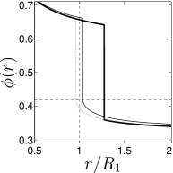
(a)

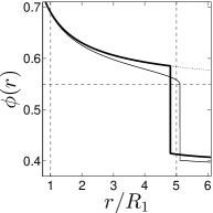
(b)

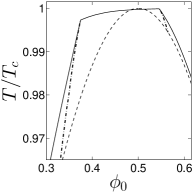
(c)

Figure 10: Electrostatic spinodal in closed systems. (a) $\phi(r)$ versus normalized $r$ for $\phi_{0}\approx 0.34$, $T/T_{c}\approx 0.973$, $\sigma=8\times 10^{-4}\,\mathrm{C/m^{2}}$, and $R_{2}/R_{1}=5$ for the minimized solution to $f$ (thick solid line) and lower metastable solution (thin solid line). Horizontal dashed line shows $\phi_{sL}$. Thick solid line also shows the minimized open system solution for $\phi_{E}=0.33$, while dotted line shows the corresponding lower solution. (b) $\phi(r)$ versus normalized $r$ for $\phi_{0}\approx 0.59$, $T/T_{c}=0.99$, $\sigma=1.46\times 10^{-3}\,\mathrm{C/m^{2}}$, and $R_{2}/R_{1}=5$ for the minimized solution to $f$ (thick solid line) and upper metastable solution (thin solid line). Horizontal dashed line shows $\phi_{sH}$. Thick solid line also shows the minimized open system solution for $\phi_{E}\approx 0.40$, while dotted line shows the corresponding upper solution. (c) Stability diagram (solid curve) with spinodal lines (dash-dotted curves) for $\sigma=8\times 10^{-4}\,\mathrm{C/m^{2}}$ and $R_{2}/R_{1}=5$. Dashed line is the binodal curve.

Material conservation produces two spinodal lines in a closed system—one line associated with each boundary. Finding the spinodal line associated with $R_{1}$ consists of finding $\phi(r_{s})=\phi_{sL}$ on the lower solution of $f$ and ensuring $r_{s}=R_{1}$, similar to open systems. However, the lower solution from $\phi_{E}$ in an open system does not fulfill the material conservation requirement. Instead, the lower solution from yet another open system concentration $\phi_{E}$ must be used. Figure 10(a) shows example $\phi(r)$ profiles associated with $R_{1}$. The heavy line corresponds to the profile $\phi(r)$ that satisfies the free energy minimum of $f$, the dotted line is the lower solution for the open system, and the thin line is the lower solution for the closed system with $R_{2}/R_{1}=5$. In Fig. 10(a), the open system could be in a metastable state (compare thick solid and dotted lines), while the closed system would not be metastable (compare thick and thin solid lines). Similar behavior applies for the location of the spinodal line at $R_{2}$; however, this line consists of finding $\phi(r_{s})=\phi_{sH}$ on the upper solution of $f$. The line styles in Fig. 10(b) are as those in Fig. 10(a). In Fig. 10(b), the closed system could be metastable, while the open system would not be metastable (recall that the upper solutions have no meaning in open systems).

Finally, Fig 10(c) shows the location of the electrostatic spinodal lines in a closed system for particular values of $\sigma$ and $R_{2}/R_{1}$. Each line begins at the critical points $(\phi_{K},T_{K})$ on either side of $\phi_{c}$ and travel down “inside” the stability diagram.

VIII Conclusion

In summary, we describe the mixing-demixing phase diagram for two dielectric liquids in an electric field. By focusing on the liquid-liquid interface and adapting standard methods for determining phase diagrams, we found the electrostatic-equivalent of binodal lines, spinodal lines, and critical points. Given this new perspective, the dynamics of phase separation with non-uniform electric fields requires reinvestigation, with an emphases on validating predicted metastable states and uncovering critical dynamic behavior. Perhaps similar adaptations of existing theory for dynamics will uncover new features in the electric-field modified liquid-liquid phase diagram.

In addition, we restricted our analysis to solutions with radial symmetry, enforcing one dimensional solutions that only depend on the distance $r$. This constraint, however, might not satisfactorily apply to all experimental conditions, and allowing for full two- or three-dimensional theoretical investigations could uncover non-radially symmetric solutions. For example, interfacial energies, both liquid-liquid and liquid-surface energies, dominate the liquid patterning for phase separation beneath the regular binodal curve in the absence of a field. And in the case where both liquids have an equal preference for the surface, liquid-liquid interfaces emerge normal to a surface. This configuration, however, can be electrostatically unfavorable since the low dielectric material is adjacent to the charge. It will be interesting to determine if, when, and how instabilities in the interface develop and if these instabilities modify the phase diagram.

Also, highly confined cylindrical geometries do not show a true liquid-liquid phase transition Winkler2010 . Here, the system can be approximated as one dimensional, with the expectation that correlations diverge as the length of the cylinder goes to infinity. It is unknown if the addition of a non-uniform electric field is sufficient to induce a true transition in this case. An appropriate investigation on this topic would, of course, require theories that go beyond the mean-field approach.

Finally, we have not considered the fluid wetting behavior on the electrode surfaces. In the wedge geometry, for example, these phenomena include wedge filling, where a liquid transitions between partial and complete filling Parry1999 ; Parry2000 ; Bruschi2002 . This transition can be either first or second order and depends on factors like the wedge opening angle, liquid contact angle, and temperature. Since our results show that the interface location directly ties with the electric field, it currently remains unclear if the electric field enhances or diminishes the effects of wetting, or possibly both (depending on experimental conditions).

Acknowledgements

This work was supported by the Israel Science Foundation under grant No. 11/10, the COST European program MP1106 “Smart and green interfaces - from single bubbles and drops to industrial, environmental and biomedical applications”, and the European Research Council “Starting Grant” No. 259205.

References

- (1) M. R. Moldover, J. V. Sengers, R. W. Gammon, and R. J. Hocken, Rev. Mod. Phys. 51, 79 (1979).
- (2) A. Asamitsu, Y. Moritomo, Y. Tomioka, T. Arima, and Y. Tokura, Nature 373, 407 (1995).
- (3) L. D. Landau and E. M. Lifshitz, Elektrodinamika Sploshnykh Sred Ch. II, Sect. 18, problem 1 (Nauka, Moscow, 1957).
- (4) A. Silberberg and W. Kuhn, Nature 170, 450 (1952).
- (5) A. I. Nakatani, F. A. Morrison, J. F. Douglas, J. W. Mays, C. L. Jackson, M. Muthukumar, and C. C. Han, J. Chem. Phys. 104, 1589 (1996).
- (6) A. Onuki, Europhys. Lett. 29, 611 (1995).
- (7) A. Onuki, Physica A 217, 38 (1995).
- (8) S. Stepanow and T. Thurn-Albrecht, Phys. Rev. E 79, 041104 (2009).
- (9) P. Debye and K. Kleboth, J. Chem. Phys. 42, 3155 (1965).
- (10) D. Beaglehole, J. Chem. Phys. 74, 5251 (1981).
- (11) M. D. Early, J. Chem. Phys. 96, 641 (1992).
- (12) D. Wirtz and G. G. Fuller, Phys. Rev. Lett. 71, 2236 (1993).
- (13) K. Orzechowski, Chem. Phys. 240, 275 (1999).
- (14) Y. Tsori, F. Tournilhac, and L. Leibler, Nature 430, 544 (2004).
- (15) G. Marcus, S. Samin, and Y. Tsori, J. Chem. Phys. 129, 061101 (2008).
- (16) S. Samin and Y. Tsori, J. Chem. Phys. 131, 194102 (2009).
- (17) A. Aharony, Phys. Rev. B 18, 3318 (1978).
- (18) R. L. C. Vink and A. J. Archer, Phys. Rev. E 85, 031505 (2012).
- (19) S. Safran, Statistical Thermodynamics of Surfaces, Interfaces, and Membranes (Westview Press, New York, 1994).
- (20) J. V. Sengers, D. Bedeaux, P. Mazur, and S. C. Greer, Physica 104, 573 (1980).
- (21) J. Leys, P. Losada-Pérez, G. Cordoyiannis, C. A. Cerdeiriña, C. Glorieux, and J. Thoen, J. Chem. Phys. 132, 104508 (2010).
- (22) M. F. Hsu, E. R. Dufresne, and D. A. Weitz, Langmuir 21, 4881 (2005).
- (23) S. Samin and Y. Tsori, J. Phys. Chem. B 115 75 (2011).
- (24) K. Binder, Spinodal Decomposition versus Nucleation and Growth, in: S. Puri and V. Wadhawan (Eds.), Kinetics of Phase Transitions, 63–99 (CRC Press, 2009).
- (25) R. Coelho and J. Debeau, J., J. Phys. D Appl. Phys 4 1266 (1971).
- (26) W. F. Schmidt, IEEE T. Electr. Insul. 19, 389 (1984).
- (27) A. Denat, J. P. Gosse, B. Gosse, IEEE T. Electr. Insul. 23, 545 (1988).
- (28) A. Winkler, D. Wilms, P. Virnau, and K. Binder, J. Chem. Phys. 133, 164702 (2010).
- (29) A. O. Parry, C. Rascón, and A. J. Wood, Phys. Rev. Lett. 83, 5535 (1999).
- (30) A. O. Parry, C. Rascón, and A. J. Wood, Phys. Rev. Lett. 85, 345 (2000).
- (31) L. Bruschi, A. Carlin, and G. Mistura, Phys. Rev. Lett. 89, 166101 (2002).