Incorporating the Hayflick Limit
into a model of Telomere Dynamics

Abstract

A model of telomere dynamics is proposed and examined. Our model, which extends a previously introduced two-compartment model that incorporates stem cells as progenitors of new cells, imposes the Hayflick Limit, the maximum number of cell divisions that are possible. This new model leads to cell populations for which the average telomere length is not necessarily a monotonically decreasing function of time, in contrast to previously published models. We provide a phase diagram indicating where such results would be expected. In addition, qualitatively different results are obtained for the evolution of the total cell population. Last, in comparison to available leukocyte baboon data, this new model is shown to provide a better fit to biological data.

I Introduction

Telomeres were first recognized in the 1930’s as special structures capping the ends of chromosomes, the cell’s genetic material. Further research has identified telomeres to be important components in a variety of cellular processes, the most important being replication Blackburn (1991). Cellular replication, known as mitosis, involves one cell dividing itself into two identical copies, each containing a full copy of the genetic material.

The replication of the cell’s linear chromosomes is a inherently destructive process, in that each replication causes a shortening of the chromosome Olovnikov (1973). Cells are able to protect their (coding) genetic material by instead allowing telomeres to shorten Blackburn (1991). As telomeres have a finite length, this puts an upper bound, called the Hayflick Limit, on the number of divisions a cell is able to undergo Hayflick and Moorhead (1961); Shay and Wright (2000). The decreasing lengths of telomeres have been found to be involved in aging, with shorter telomeres associated with advanced age, and the mortality of an organism associated with the finite length of the telomere.

While all cells contain chromosones and telomeres, there are only a select few cell types that are actively dividing throughout adulthood. Most other cells instead have lifetimes on the same order as the organism itself, and thus divide rarely or not at all. Leukocytes, or white blood cells, are among the few cell types that regularly divide. Leukocytes encompass multiple different types of mononucleated blood cells including lymphocytes, viz. B cells and T cells, as well as granulocytes. These cells are involved in the cellular component of immune response, and thus they experience large cellular turnover and are required to maintain large, dynamic populations. The ease with which leukocytes can be extracted and analyzed, especially when compared to other rapidly dividing cell types, such as colon crypt cells, makes them the perfect subject for analyzing the Hayflick limit and telomere length dynamics.

All blood cells, white or red, originate as hematopoietic stem cells within the bone marrow. These stem cells are pluripotent, self-renewing cells capable of differentiating into unique types of hematopoietic progenitor cells, which then mature into peripheral blood cells Sidorov et al. (2009). The hematopoietic stem cells are considered to be “immortal cells”, and are believed to maintain their telomere length by means of the enzyme telomerase. The kinetics of T cells and other leukocytes has been studied extensively, and values have been obtained for their proliferation and the death rates. Estimated values are shown in Table 1.

Cell Type	Mitotic Rate (/week)	Death Rate (/week)
Memory T-Cells Borghans and de Boer (2007)	0.02 - 0.03	0.02 - 0.03
Mature B-Cells Cooperman et al. (2004)	0.5	0.48
Neutrophiles Summers et al. (2010)	0.042	0.042

Table 1: Estimated values from the literature for the mitotic and death rates for (memory) T cells, (memory) B cells and (neutrophiles) granulocytes.

As cells divide and multiply the end-replication problem causes chromosomal shortening. The level of attrition in leukocytes has been measured and most estimates of the number of base pairs lost per division range from 50 to 100 bp, with the highest estimate at 120 bp/division Weng et al. (1995); Vaziri et al. (1993). This value is not uniform across species or even between individuals, with the exact figure changing greatly between individuals and different cells types. As telomeres are of a finite length, the chromosonal loss that each mitotic cycle causes results in the Hayflick limit, the theoretical maximum number of divisions a cell may undergo. Leukocytes were found to be able to divide on average 23 times before reaching senescence Pilyugin et al. (1997). Similiar to the amount of base pairs lost per cell division, the Hayflick limit varies greatly among different cell types. For human fibroblasts between 14 and 29 divisions were observed, while for human embryos the limit was found to be between 35 and 63 divisions Hayflick and Moorhead (1961).

I.1 Outline of Paper

In the next section we state and put into context previously published dynamical models of telomere shortening. Using for now a minimalist’s approach, we restrict our attention to the simplest linear dynamical models, as our goal is to report on the dynamics that results from the incorporation of the Hayflick Limit into such minimalist models. We compare our results to previously published work and find one new feature – a phase transition occurs in terms of the qualitative behaviour of the mean telomere length. Then we discuss the application of our model to experimental data on baboon leukocytes, and show that one obtains an improved fit to this data using our model. Finally, we discuss how this model can be related to aging and cancer and other aspects of chromosomal length dynamics.

II Summary of Previous Dynamical Models

We briefly review previously studies models below, allowing us to define our notation, and to allow for a direct comparison of our work with previously published theories.

II.1 Single compartment model

Our introduction highlights that the majority of situations in which dividing cells are encountered, such as leukocytes, involve a stem cell population replenishing a population of (white blood) cells. If one ignores the stem cells, one may model the simpler situation of a population of cells dividing and dying DeBoer and Noest (1998).

Let $i(t)$ denote the number of divisions that a cell has undergone at time $t$, and let $N_{i}(t)$ denote the number of such cells in the population. If the rate of mitotic division is denoted by $M$, and the rate of cell death by $D$, allowing for potentially an infinite number of cell divisions, one simply has

$$\dot{N}_{0}~{} = ~{}-(M+D)~{}N_{0}$$

$$\dot{N}_{i}~{} = ~{}2M~{}N_{i-1}~{}-(M+D)~{}N_{i}~{}~{}~{}~{}~{}~{}~{}i=1,2,\dots$$ (1)

Assuming that

$$N_{i}(0)~{}=~{}N_{o}^{o}~{}\delta_{i,0}$$ (2)

the total number of cells in this model, denoted by $\mathcal{N}(t)=\sum_{i}N_{i}(t)$, is easily found to be

$$\mathcal{N}(t)~{}=~{}N_{o}^{o}~{}e^{(M-D)t}$$ (3)

If $D>M$ the total number of cell decreases with time, as expected physically. However, for $D>M$ the total cell population diverges in this model. Note that Table 1 does not make clear which inequality is to be expected, and we discuss this result below.

The average number of cell divisions undergone in such a cell population is found through the use of the generating function Berg (1978)

$$\mathcal{F}(x,t)~{}=~{}\sum_{i}~{}x^{i}~{}N_{i}(t)$$ (4)

whose ODE (derivative with respect to time) is easily solved using the original equations of motion. That is (using the same initial conditions),

$$\overline{i}(t)~{}=~{}\frac{1}{\mathcal{N}(t)}~{}\sum_{j}~{}j~{}N_{j}(t)~{}=~{}\frac{1}{\mathcal{N}(t)}~{}\frac{\partial\mathcal{F}}{\partial x}|_{x=1}~{}=~{}2Mt$$ (5)

Let $L(t)$ denote the length of a chromosome at time $t$. Define the initial length of a chromosome’s telomere to be $L_{o}$, and suppose that, on average, the number of base pairs lost from the telomeres in each mitotic event is given by $\Delta_{o}$. Then

$$\overline{L}(t)~{} \equiv \frac{1}{\mathcal{N}(t)}\Big{(}N_{0}L_{o}~{}+~{}N_{1}(L_{o}-\Delta_{o})~{}+~{}N_{2}(L_{o}-2\Delta_{o})~{}+~{}\dots\Big{)}$$ (6)

$$= ~{}L_{o}~{}-~{}\Delta_{o}~{}\overline{i}(t)$$

giving that for this one-compartment model

$$\overline{L}(t)~{}=~{}L_{o}~{}-~{}\Delta_{o}~{}2Mt$$ (7)

This shows that, on average, in this simple single compartment model the length of a telomere decreases linearly with time. This generates the unphysical result that Eq. (7) predicts that eventually the length of a telomere is negative.

Below we contrast our results with these results, in particular Eqs. (3,7).

II.2 Two compartment model without the Hayflick Limit

The work of Itzkovitz et al. Itzkovitz et al. (2008) advanced that of the previous subsection by including a second compartment, the latter associated with a population of stem cells that replenish the population of cells under study. The modification of the above model in one sense is very minor, namely the equations of motion now become

$$\dot{N}_{0}~{} = ~{}\alpha-(M+D)~{}N_{0}$$

$$\dot{N}_{i}~{} = ~{}2M~{}N_{i-1}~{}-(M+D)~{}N_{i}~{}~{}~{}~{}~{}~{}~{}i=1,2,\dots$$ (8)

where $\alpha$ corresponds to the rate at which the stem cells are producing new cells. It is assumed that all nuclei produced by stem cells have telomeres of length $L_{o}$. However, a more substantive change was made in that $\alpha$ is chosen to maintain a constant cell population size (independent of the distribution of telomere lengths), this condition corresponding to

$$\alpha~{}=~{}(D-M)~{}N_{o}^{o}$$ (9)

(This result is for the same initial condition as given in Eq. (2); more generally, a constant total cell population is found for $\alpha~{}=~{}(D-M)~{}N_{o}$ , where $N_{o}$ is the total population of all cells at $t=0$.) As shown in that paper, again utilizing the generating function of Eq. (4), one then obtains that the average length of the telomeres follows

$$\overline{L}(t)~{}=~{}L_{o}~{}-~{}\Delta_{o}\frac{2MN_{o}^{o}}{\alpha}~{}\big{(}1-e^{-(\alpha~{}t/N_{o}^{o})}\big{)}$$ (10)

We see that while this two-compartment model includes the unphysical situation of having telomeres with a negative length, the result for the average telomere length now remains positive when

$$L_{o}~{}>~{}\Delta_{o}\frac{2MN_{o}^{o}}{\alpha}$$ (11)

Moreover, for small times one obtains

$$\overline{L}(t\approx 0)~{}=~{}L_{o}~{}-~{}\Delta_{o}~{}2Mt$$ (12)

which is the same result as is found for the one-compartment model in Eq. (7).

We have also analysed this model without the imposition of a fixed population size – that is, for which Eq. (9) is not satisfied. Using the initial condition of Eq. (2), one obtains

$$\mathcal{N}(t)~{}=~{}N_{o}^{o}~{}e^{(M-D)t}~{}+~{}\frac{\alpha}{M-D}~{}\big{(}e^{(M-D)t}~{}-~{}1\big{)}$$ (13)

which is the similar to the one-compartment model – see Eq. (3) – with the added effect of the stem cell pool. Note again that for $M>D$, like the one-compartment model, this expression diverges for large times. In addition, one can derive the expression for the average telomere length. This expression is cumbersome, but its behaviour can be identified for small and long times, namely

$$\overline{i}(t)\sim\begin{dcases*}~{}~{}2Mt&for $t\approx 0^{+}$\\ ~{}~{}2Mt&for $t\rightarrow\infty$ and $M>D$\\ ~{}~{}\frac{2M}{D-M}&for $t\rightarrow\infty$ and $D>M$\end{dcases*}$$

Note the similarity of this results, when $M>D$, to the one-compartment model result of Eq. (5). Most importantly, one may show that $\overline{i}(t)$ for the two-compartment model without a fixed total population is a monotonically increasing function of time, regardless of the sign of $M-D$.

III Incorporating the Hayflick Limit in a Two-Compartment Model

III.1 Dynamical System of Equations

We modify the two-compartment model as follows. We assume that after mitosis has occurred a fixed number of times, the Hayflick limit, which we denote by $h$, the cells become senescent. For simplicity, we assume that the death rate of the senescent cells is the same as that for any other cells, although it is simple to relax this assumption. The resulting dynamical system of equations is therefore

$$\dot{N}_{0}~{} = ~{}\alpha-(M+D)~{}N_{0}$$

$$\dot{N}_{i}~{} = ~{}2M~{}N_{i-1}~{}-(M+D)~{}N_{i}~{}~{}~{}~{}~{}~{}~{}i=1,2,\dots,h-1$$ (14)

$$\dot{N}_{h}~{} = ~{}2M~{}N_{h-1}~{}-~{}D~{}N_{h}~{}~{}$$

As discussed in the introduction, the biologically relevant values for $h$ are between 14 and 63, and for human leukocytes a value of $h=23$ has been measured. This system of equations is easily solved for any $h$, simply by iteration. However, it is easiest to work with a scaled system of equations, as we now discuss.

One can reduce Eq. (III.1) to a sequence of dimensionless rate equations, and similarly dimensionless parameters. To do so we redefine the generational populations, $N_{i}$ in terms of a new set of scaled populations, $f_{i}$, as follows. Let

$$N_{i}~{} = ~{}a_{i}~{}f_{i}~{}~{}~{}~{}~{}~{}i=0,1,2,\dots,h~{}~{}~{}~{}~{}~{}~{}$$ (15)

$$t~{} = ~{}b~{}\tau$$

and choosing

$$a_{i}=\Big{(}\frac{2M}{M+D}\Big{)}^{i}\Big{(}\frac{\alpha}{M+D}\Big{)}~{}~{}~{}~{}~{}i=0,1,2,\dots,h~{}~{}~{}~{}~{}~{}~{}b=(M+D)^{-1}$$ (16)

the system of equation governing the generational populations then reduce to the much simpler form

$$\frac{d}{d\tau}f_{0}(\tau) = 1-f_{0}(\tau)$$

$$\frac{d}{d\tau}f_{I}(\tau) = f_{I-1}(\tau)-f_{I}(\tau)~{}~{}~{}~{}~{}~{}~{}~{}~{}~{}I=1,2,\dots,h-1$$ (17)

$$\frac{d}{d\tau}f_{h}(\tau) = f_{h-1}(\tau)-\gamma~{}f_{h}(\tau)$$

where

$$\gamma\equiv\frac{D}{D+M}$$ (18)

Using the initial condition of Eq. (2) we see that solution of Eq. (III.1) depends on only three dimensionless parameters, namely

$$f_{o}^{o}~{}\equiv~{}\frac{M+D}{\alpha}~{}N_{o}^{o}$$ (19)

$\gamma$ and, of course, $h$. Below we investigate the dynamics of this model subject to variations in these quantities.

For completeness, we note that steady-state solutions of these equations are then trivially seen to be

$$f_{I}(\infty)=1~{}~{}~{}~{}~{}~{}~{}~{}I=0,1,\dots,h-1,~{}~{}~{}~{}~{}~{}~{}~{}~{}f_{h}(\infty)=\frac{1}{\gamma}$$ (20)

Clearly, the introduction of the scale factors of Eq. (16) dramatically simplifies the considerations of the statics of this problem. (Nonlinear aspects of the steady-state solutions found when the rate constants are modelled with Hill functions, etc, were considered by others Pilyugin et al. (1997).)

III.2 Phase Diagram of Dynamical Solutions

As mentioned above, one may solve the system of equations iteratively. However, as is apparent from Eq. (III.1) it is simplest to integrate the scaled equations. Expressions for $f_{I}$ for $I=0,\dots,h-1$ can be written down, namely

$$f_{o}(\tau) = e^{-\tau}\big{(}f_{o}^{o}-1+e^{\tau})$$

$$f_{1}(\tau) = e^{-\tau}\big{(}f_{o}^{o}~{}t-1-t+e^{\tau})$$

$$f_{2}(\tau) = e^{-\tau}\big{(}f_{o}^{o}~{}t^{2}-2t-t^{2}+2e^{\tau})$$ (21)

$$f_{3}(\tau) = \dots$$

The expression for $f_{h}(\tau)$ is long and complicated (even for $h=5$ – see below) so we refrain from providing it. A formal closed-form solution for related equations may be obtained, if desired Gyllenberg (1986). (Analytical expressions found from the integration of these coupled ODE’s using Laplace transforms, or a computer algebra software, such as Mathematica^©, can be obtained in a straightforward manner.) Here we show how two qualitatively different classes of solutions exist, one of which is not found in either the one compartment model, or the two-compartment model without the Hayflick limit.

Figure 1: The behaviour of the (scaled) populations, $f_{I}(\tau)$, $I=0,1,2,3,4,5$, for $\gamma=0.55$ for (a) $f_{o}^{o}=1.5$ and (b) $f_{o}^{o}=5$. In the first figure one sees that the populations (for $I>0$) increase monotonically with $\tau$, whereas in the second figure (for $I>0$) the populations achieve a local maximum.

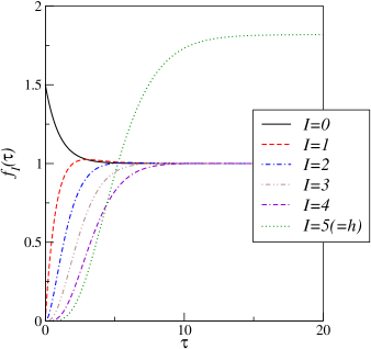
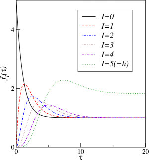
To be concrete, consider $h=5$; similar behaviour is found for larger $h$, but here we choose this small value to make the presentation of our results simpler. It is clear that on biological grounds we expect $\gamma\approx 1/2$ since $D\approx M$. Therefore, we show the solution of $f_{I}(\tau)$ for $I=0,1,...,5$ for $\gamma=0.55$ for two values of $f_{o}^{o}$, namely $f_{o}^{o}=1.5$ and 5. Our results are shown in Fig. 1 (note that qualitatively similar results are found when $\gamma=0.45$, corresponding to $D<M$). For the smaller value of $f_{o}^{o}$ the (scaled) populations for $I=1,2,\dots,h$ all increase monotonically with time, whereas for the larger value of $f_{o}^{o}$ the populations all show a local maximum (located at different $\tau$ for each $f_{I}$). The appearance of these local maxima could be important in the interpretation of biological experiments, as we now describe.

Figure 2: The variation in the average number of cell divisions in the (scaled) population of cells - see Eq. (22). The maximum number of divisions is $h=5$, we chose $\gamma=0.55$, and the curves are for small $f_{o}^{o}(=1.5)$ (solid line) and large $f_{o}^{o}(=5)$ (dashed line). Similar results are found for $\gamma=0.45$, but as discussed in the text, the appearance or absence of a local maximum in $\overline{I}(\tau)$ is dependent on the choice of $h$, $\gamma$ and $f_{o}^{o}$.

These model equations were motivated by the behaviour of telomere lengths as individuals age. Therefore, it is important to consider the average number of cell divisions that are found for these (scaled) populations. This latter quantity is given by

$$\overline{I}(\tau)~{}=~{}\frac{\sum_{I=0}^{h}~{}I~{}f_{I}(\tau)}{\sum_{I=0}^{h}~{}f_{I}(\tau)}$$ (22)

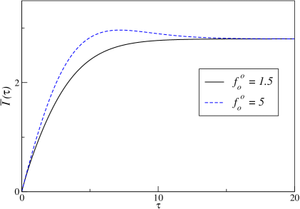
As seen in Fig. 2, for small $f_{o}^{o}$ this function increases monotonically with time, whereas for larger $f_{o}^{o}$ one obtains a local maximum at an intermediate time. The importance of this result is seen when considered with the definition of the average telomere length $\overline{L}(t)$ – see Eq. (6). That is, one can now obtain a local minimum for this quantity, and this could lead to significant differences when fitting (e.g., leukocyte) telomere data, as we describe in the next section. (We have confirmed this behaviour of $\overline{L}(t)$ for a variety of different parameter values.)

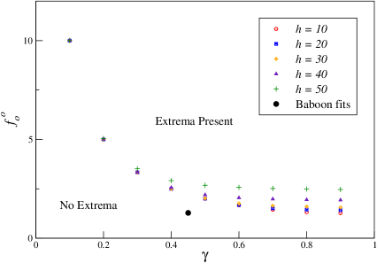
The above result raises an interesting question: How does the appearance of a local maximum in $\overline{I}(t)$ (or a local minimum in $\overline{L}(t)$) depend on the value of the Hayflick limit, $h$? It’s clear that in the $h\rightarrow\infty$ limit one recovers the two-compartment model discussed above, and when a constant total population size is enforced via the imposition of Eq. (9), from Eq. (10) one sees that this produces a monotonically decreasing $\overline{L}(t)$ without any local maximum. Therefore, our simple linear model incorporating the Hayflick limit possesses a transition in that for finite $h$ and fixed $\gamma$, at small $f_{o}^{o}$ no extrema appear in the dynamics, whereas for larger $f_{o}^{o}$ extrema do appear. One can therefore identify critical parameters $(\gamma,f_{o}^{o})$ for each $h$ separating these qualitatively different dynamics. It is a simple manner to do this numerically.

Figure 3: A phase diagram showing how the average (scaled) telomere length of Eq. (22) depends on the the maximum number of cell divisions, $h$ (the Hayflick Limit), $\gamma$, and $f_{o}^{o}$. Above the phase boundary for each $h$, $\overline{I}(t)$ has a local minimum, whereas below the phase boundary no extrema are present. As $h$ increases the region that includes an extremum in $\overline{I}(t)$ diminishes, and eventually this region vanishes as $h\rightarrow\infty$. The large solid circle shows the average values of these parameters when fitted to baboon leukocyte data – see §IV for a discussion of this result.

We have completed this analysis for $h=10,20,30,40,50$, and our results are shown in Fig. 3. As expected based on the above-studied two-compartment model (see section 2.1 of this paper), as $h$ increases the parameter regime over which one finds dynamics possessing extrema is found to shrink, and eventually this region must vanish in the $h\rightarrow\infty$ limit. This analysis can also be completed for the unscaled populations $N_{i}(t)$ and a phase diagram found in terms of $\overline{L}(t)$; our numerical result for such a calculation is that the resulting phase diagram is identical to that of Fig. 3.

IV Application to Leukocyte Data

In Ref. Itzkovitz et al. (2008) the two-compartment model with fixed population size was compared to experimental data Baerlocher et al. (2007) for 3 different baboons (subjects 17891, 17927 and 18760) for 3 different leukocytes - B cells, T cells, and granulocytes. (Note that we confirmed numerically that this model represents an improvement over the one-compartment model of Ref. DeBoer and Noest (1998).) Therefore, we then compared our model, which incorporates the Hayflick limit, to this same data set. For our comparison we used $h=23$, based on Ref. Pilyugin et al. (1997), although our results are not sensitive to small changes in $h$ (that is, $h=20$ to $h=26$ all give very similar fits). We find that fitting this same data with our Hayflick Limit model leads to a small reduction (6%) in the mean square differences of the data and fitted functions relative to Ref. Itzkovitz et al. (2008).

For all three baboons and and all three leukocytes, our results for the fitted parameters correspond to the “No Extrema” portion of our dynamical phase diagram. Averaging values of $\gamma$ and $f_{o}^{o}$ over the three different baboons and the three different leukocytes gives

$$\overline{f}_{o}^{o}~{}=~{}1.29\pm 0.16~{}~{}~{}~{}~{}~{}~{}~{}~{}~{}~{}~{}~{}\overline{\gamma}~{}=~{}0.46\pm 0.04$$

showing that very similar parameters fit all of the experimental data sets. These average values are included on Fig. 3, showing that for this $h=23$ dynamical system indeed no extremal dynamics are encountered.

Other interesting biological information contained in these fits (rate constants in units of inverse weeks) is as follows.

• The initial lengths, $L_{o}$, of the telomeres are different for different baboons, but do not vary as much between different leukocytes.

• The shortening of the telomeres per mitotic division, $\Delta_{o}$, strongly varies between leukocytes for a given baboon, as well as showing strong variation between baboons.

• In all cases the fitted values of the death and mitotic division rates are similar in that $0.39\lesssim\gamma\lesssim 0.54$, showing that $D$ is similar to but somewhat smaller than $M$. This result is similar to the previously published work summarized in our Table 1.

• The rates at which the stem cells replenish the leukocytes are remarkably similar: $390\lesssim\alpha\lesssim 396$.

V Summary and Discussion

The dynamical equations describing telomere shortening are certain to be complicated. We have modelled this biology in terms of the number of cells in a population which have undergone a given number of cell divisions up to a maximum number of divisions, called the Hayflick Limit. We have taken a minimalist’s approach in using simple linear equations of motion. Our reason is nothing more than wanting to identify the different qualitative dynamics that result from such a “bare bones” model. Then, when new complications are added to these equations, such as the effects of telomerase, etc., new biological behaviours can hopefully more clearly be identified.

Our model is a modification of the work of two-compartment model of Ref. Itzkovitz et al. (2008), which itself is an extension of the one-compartment model of Ref. DeBoer and Noest (1998). In a two-compartment model one accounts for the presence of stem cells as being the progenitors of new cells with chromosomes having full-length telomeres. Both of these models, viz. Eqs. (II.1,II.2), suffer from the unphysical populations of negative length telomeres that are produced, a byproduct of these models not accounting for the Hayflick limit. Our model limits the total number of mitotic events that can occur to a set of chromosomes, and therefore accounts for the Hayflick limit. One may analytically solve the resulting set of dynamical equations for the cell populations, and from this calculate, for example, the average length of telomeres as a function of time.

The interesting result that follows from our model is shown in Fig. 2. That is, our model, given in Eq. (III.1), can produce an average telomere length that decreases with time, reaches a local extremum, and then increases with time until some steady-state value is reached. The biological importance of such a result can be reasoned as follows. In an experimental study of telomere lengths, if data is found that shows such non-monotonic behaviour, it would not necessarily be correct to attribute such data to new biology, such as the lengthening of telomeres by telomerase (or ALT, or other chromosome altering events). Instead, the simplest dynamical equations that incorporate senescence and the Hayflick limit are sufficient to give such a result. We have compared the resulting expression for average telomere length to published data, and reasonable agreement is found, being, in fact, somewhat of a better fit than is found using the previously published two-compartment model with a fixed population size.

As the above discussion foreshadows, the work presented in this paper is but a first step at addressing the complicated biology associated with telomere shortening. Future work will investigate biology such as that found in malignant cancerous cells, otherwise known as “immortal cells”, leading to uncontrolled growth of tumours. Noting that early work on this problem Kim et al. (1994) reported that in all tumour cells lines, and in 90% of all primary tumour samples (from biopsies) telomerase is present, modelling the feedback of this enzyme on chromosome biology deserves further attention.

References

- Blackburn (1991) E. Blackburn, Science 35, 569 (1991).
- Olovnikov (1973) A. Olovnikov, J Theor Biol 41, 181 (1973).
- Hayflick and Moorhead (1961) L. Hayflick and P. Moorhead, Exp Cell Res 25, 585 (1961).
- Shay and Wright (2000) J. Shay and W. Wright, Nature Reviews Molecular Cell Biology 1, 72 (2000).
- Sidorov et al. (2009) I. Sidorov, M. Kimura, A. Yashin, and A. Aviv, Experimental Hematology 37, 514 (2009).
- Borghans and de Boer (2007) J. Borghans and R. de Boer, Immunological Reviews 216, 35 (2007).
- Cooperman et al. (2004) J. Cooperman, R. Neely, D. Teachey, S. Gruppe, and J. Choi, Stem Cells 22, 1111 (2004).
- Summers et al. (2010) C. Summers, S. Rankin, A. Condliffe, N. Singh, A. Peters, and E. C. ER, Trends in Immunology 31, 318 (2010).
- Weng et al. (1995) N.-P. Weng, B. Levine, C. June, and R. Hodes, Proc Natl Acad Sci (USA) 92, 11091 (1995).
- Vaziri et al. (1993) H. Vaziri, F. Schachter, I. Uchida, L. Wei, X. Zhu, R. Effros, D. Cohen, and C. Harley, Am J Hum Genet 52, 661 (1993).
- Pilyugin et al. (1997) S. Pilyugin, J. Mittler, and R. Antia, J Theor Biol 186, 117 (1997).
- DeBoer and Noest (1998) R. DeBoer and A. Noest, J Immunol 160, 5832 (1998).
- Berg (1978) O. Berg, J Theor Biol 71, 587 (1978).
- Itzkovitz et al. (2008) S. Itzkovitz, L. Shlush, D. Gluck, and K. Skorecki, Phys Rev E 78, 060902 (2008).
- Gyllenberg (1986) M. Gyllenberg, J Math Biol 24, 81 (1986).
- Baerlocher et al. (2007) G. Baerlocher, K. Rice, I. Vulto, and P. Lansdorp, Aging Cell 6, 121 (2007).
- Kim et al. (1994) N. Kim, N. Piatyszek, K. Prowse, C. Harley, M. West, P. Ho, G. Coviello, W. Wright, S. Weinrich, and J. Shay, Science 266, 2011 (1994).