Zeno Dynamics and High-Temperature Master Equations Beyond Secular Approximation

Abstract

Complete positivity of a class of maps generated by master equations derived beyond the secular approximation is discussed. The connection between such class of evolutions and physical properties of the system is analyzed in depth. It is also shown that under suitable hypotheses a Zeno dynamics can be induced because of the high temperature of the bath.

1 Introduction

Quantum Zeno effect (QZE) is an ubiquitous phenomenon in quantum mechanics [1, 2, 3, 4], relevant in the analysis of fundamental concepts of quantum mechanics [5, 6, 7, 8], useful in applications [9], and which has been experimentally demonstrated [10, 11, 12].

Recently, the connection between occurrence of Zeno phenomena and the properties of the environment of the physical system under scrutiny has been investigated [13, 16, 14, 15]. The connection between QZE and high-temperature has been studied. Inhibition of Landau-Zener transitions induced by temperature has been predicted [17], and enhancement of QZE phenomena through temperature has been analyzed in depth [18]. In the case of high temperature, exploitation of the standard approach to derive master equations, and consequent secular approximation could be problematic, due to the fact that in such a case the secular approximation, generally performed after Born-Markov approximation, can be inappropriate because of an effectively high coupling strength induced by the increased number of photons. Nevertheless, in general, avoiding secular approximation would produce a generator of a non-completely positive map. Since complete positivity is a necessary condition for a map describing a physical system [19], one needs to overcome such difficulty. Studies of quantum optics models obtained beyond the secular approximation or without the rotating wave approximation (two names used in different contexts to address essentially the same approximation) have been reported through the years in different papers [20].

In this paper, we find suitable hypotheses under which Markovian approach, in the limit of high temperature, can produce a completely positive map even beyond the secular approximation. Moreover, through the master equation derived along this route, it is possible to forecast the occurrence of a Zeno phenomenon under suitable hypotheses. This outcome somehow confirms the results obtained in [17] and [18]. The paper is organized as follows. In the next section we introduce the general approach and assumptions to derive the master equation in the high temperature limit beyond the secular approximation. In section 3 we provide a general statement connected with the appearance of Zeno phenomena, and show an example in a three-level system where the high temperature master equation clearly forecasts preservation of a subspace, which we address as thermal quantum Zeno effect. Finally, in the last section, we give some conclusive remarks.

2 Master Equation

Let us consider a system interacting with a bosonic environment:

$$H_{\mathrm{S}} = \sum_{\epsilon}\epsilon\Pi(\epsilon)\,,$$ (1)

$$H_{\mathrm{B}} = \sum_{k}\omega_{k}a^{\dagger}_{k}a_{k}\,,$$ (2)

$$H_{\mathrm{I}} = A\otimes B\,,\qquad B=\sum_{k}\left(g_{k}^{*}a_{k}+g_{k}a_{k}^{\dagger}\right)\,,$$ (3)

where $\Pi(\epsilon)$ are projectors on eigenspaces of $H_{\mathrm{S}}$ and $A=A^{\dagger}$.

Now, following the standard approach [22, 21], in the weak coupling limit, we can assume that the total density matrix can be separated in the system and bath degrees of freedom (Born approximation): $\rho_{\mathrm{T}}=\rho\otimes\rho_{\mathrm{B}}$, where $\rho$ is the density operator of the system $\mathrm{S}$ and $\rho_{\mathrm{B}}$ is the thermal state of the bosonic bath — the state of the bath does not significantly change, both because of the weak coupling limit and the fact that the environment is much larger than the system and therefore negligibly affected by it. Then we formally integrate the von Neumann equation, iterate it and differentiate both members of the relation obtained:

$$\frac{\mathrm{d}\rho(t)}{\mathrm{d}t}=-\int_{0}^{t}\,\mathrm{d}s\,\mathrm{tr}_{\mathrm{B}}\,[H_{I}(t),[H_{I}(s),\rho(s)\otimes\rho_{\mathrm{B}}]]\,,$$ (4)

where, considered the structure of the operator $B$ and of the thermal state $\rho_{\mathrm{B}}$, one has $\mathrm{tr}_{\mathrm{B}}[\rho_{\mathrm{B}},B]=0$.

Subsequently, we perform the Markov approximation by substituting the density operator $\rho(s)$ in the integral with $\rho(t)$, and then (by assuming very short correlation time for the bath) we put the second limit of integration to infinity:

$$\frac{\mathrm{d}\rho(t)}{\mathrm{d}t}=-\int_{0}^{\infty}\,\mathrm{d}s\,\mathrm{tr}_{\mathrm{B}}\,[H_{I}(t),[H_{I}(t-s),\rho(t)\otimes\rho_{\mathrm{B}}]]\,.$$ (5)

Then we introduce the jump operators:

$$A(\omega) =\sum_{\epsilon^{\prime}-\epsilon=\omega}\Pi(\epsilon)\,A\,\Pi(\epsilon^{\prime})\,,$$ (6)

where the sum is meant over all $\epsilon$ and $\epsilon^{\prime}$ such that $\epsilon^{\prime}-\epsilon=\omega$. By exploiting such operators and before performing the secular approximation, we obtain:

$$\frac{\mathrm{d}\rho}{\mathrm{d}t} = -i\left[H_{\mathrm{S}},\rho\right]+\sum_{\omega,\,\omega^{\prime}}\,\,\,\Gamma(\omega)\left[A(\omega)\rho\,A^{\dagger}(\omega^{\prime})-A^{\dagger}(\omega^{\prime})A(\omega)\rho\right]+\mathrm{H.c.}\,,$$

with $\omega$ and $\omega^{\prime}$ spanning over all possible Bohr frequencies of the system, and

$$\Gamma(\omega) = \int_{0}^{\infty}\mathrm{d}s\,e^{i\omega s}\mathrm{tr}_{B}\left[B^{\dagger}(t)B(t-s)\rho_{B}(0)\right]\,$$ (10)

$$= \left\{\begin{array}[]{ll}\left|g(\omega)\right|^{2}D(\omega)(1+N(\omega))\,,&\omega>0\\ &\\ \left|g(|\omega|)\right|^{2}D(|\omega|)\,N(|\omega|)\,,&\omega<0\,,\end{array}\right.$$

where $D(\omega)$ is the bath density of modes, while $g(\omega)$ is the coupling constant $g_{k}$ in the continuum limit, and $N(\omega)=1/(\exp(\hbar\omega/(k_{B}T)-1)$. In the derivation of Eq.(2) we have neglected the Lamb shifts (LS), which, on the other end, if not negligible can be absorbed by the commutator after introducing $\tilde{H}_{\mathrm{S}}=H_{\mathrm{S}}+\mathrm{LS}$ and $[H_{\mathrm{S}},\rho]\rightarrow[\tilde{H}_{\mathrm{S}},\rho]$.

Generally, Eq.(2) does not define the generator of a completely positive map. What one usually does is to perform the secular approximation in order to find a completely positive generator. This implies keeping only the diagonal terms ($\omega=\omega^{\prime}$) in Eq. (2) and neglecting the rest.

Anyway, as we are going to demonstrate, there exist suitable hypotheses under which the structure of the Markovian master equation without secular approximation approaches a generator of a CP map.

Assume that there are two subspaces, say $1$ and $2$, corresponding to two projectors $\Pi_{1}$ and $\Pi_{2}$ generated by projectors on eigenspaces of $H_{\mathrm{S}}$. Assume also that the operator $A$ connects only such two subspaces, which means:

$$\Pi_{1}\,A\,\Pi_{1}=0\,,\qquad\Pi_{2}\,A\,\Pi_{2}=0\,,$$ (12)

$$\Pi_{1}\,A\,\Pi_{2}\not=0\,,\qquad\Pi_{2}\,A\,\Pi_{1}\not=0\,.$$ (13)

Eqs.(12) express the fact that $A$ does not induce transitions within each of the two subspaces (all matrix elements involving any couple of states of the same subspace are vanishing). Transitions from one subspace to the other are instead allowed, according to eqs.(13). In Fig. 1 we provide a graphical representation of this scenario. If $\omega$ refers to a transition within $\Pi_{1}$ or within $\Pi_{2}$, then the corresponding $A(\omega)$ vanishes, due to Eq.(12). Instead, if $\omega$ refers to transitions between the two subspaces then the corresponding $A(\omega)$ is non-vanishing. All this implies that in Eq.(2) summation can be restricted to $\omega$ and $\omega^{\prime}$ lying in the inter-band transition frequencies (frequencies related to transitions from $\Pi_{1}$ to $\Pi_{2}$ and vice versa). Let us introduce $\omega_{0}$ as the frequency connecting the centre of the band associated to $\Pi_{1}$ with the centre of the band associated to $\Pi_{2}$. We will use the notation $\sum_{\omega\sim\omega_{0}}$ to indicate summation over values of $\omega$ (whose absolute values are) close to $\omega_{0}$.

Assume also that the Bohr frequencies related to transitions from any state in $\Pi_{1}$ to any state in $\Pi_{2}$ are much larger than the Bohr frequencies associated either to transitions inside $\Pi_{1}$ or to transitions inside $\Pi_{2}$.

Finally, assume that the spectrum is flat, meaning that $\left|g(|\omega|)\right|^{2}D(|\omega|)=\gamma$ is independent of $\omega$, at least in a neighborhood of $\omega_{0}$ corresponding to the frequencies of interest for this physical problem. Of course, $\Gamma(\omega)$ still contains a dependence on $\omega$ due to the term $N(\omega)$.

Now, in the limit of high-temperature (which implies $N(\omega)\gg 1$) and weak coupling ($\gamma\rightarrow 0$), we can consider $\gamma(1+N(\omega))\approx\gamma N(\omega)$. Moreover, in the high-temperature limit it turns out $N(\omega)\approx k_{B}T/(\hbar\omega)$, and since the frequencies connecting the subspaces $1$ and $2$ are very close — they are all much larger than the Bohr frequencies associated to transitions internal to each subspace — then one can deduce that $N(\omega)$ does not significantly depend on $\omega$, when $\omega$ is related to a transition between the two subspaces. In particular, one has ($\omega=\omega_{0}+\delta\omega$)

$$N(\omega) \approx N(\omega_{0})+\left.\frac{\partial N}{\partial\omega}\right|_{\omega=\omega_{0}}\delta\omega$$ (14)

$$= N(\omega_{0})-[N(\omega_{0})]^{2}\,\exp\left({\frac{\hbar\omega_{0}}{k_{\mathrm{B}}T}}\right)\frac{\hbar\delta\omega}{k_{\mathrm{B}}T}$$

$$\approx N(\omega_{0})-\frac{k_{\mathrm{B}}T\delta\omega}{\hbar\omega_{0}^{2}}\,,$$

where the last step is legitimated at high temperature, since in this limit $N(\omega_{0})\approx k_{\mathrm{B}}T/(\hbar\omega_{0})$ and the exponential $\exp(\hbar\omega_{0}/(k_{\mathrm{B}}T))$ approaches unity.

Therefore, Eq.(2) may be cast in the following form:

$$\frac{\mathrm{d}\rho}{\mathrm{d}t} \approx-i\left[H_{\mathrm{S}},\rho\right]+\gamma\left\{\sum_{\omega,\,\omega^{\prime}\sim\omega_{0}}\,\,\,N(\omega)\left[A(\omega)\rho\,A^{\dagger}(\omega^{\prime})-A^{\dagger}(\omega^{\prime})A(\omega)\rho\right]+\mathrm{H.c.}\right\}\,$$ (15)

$$\approx-i\left[H_{\mathrm{S}},\rho\right]+\gamma N(\omega_{0})\left\{\sum_{\omega,\,\omega^{\prime}\sim\omega_{0}}\,\,\,[A(\omega)\rho\,A^{\dagger}(\omega^{\prime})-A^{\dagger}(\omega^{\prime})A(\omega)\rho]+\mathrm{H.c.}\right\}$$

$$+\gamma\,O(k_{\mathrm{B}}T\delta\omega/(\hbar\omega_{0}^{2}))\,.$$

Since $A=\sum_{\omega}A(\omega)=$ $\sum_{\omega\sim\omega_{0}}A(\omega)=$ $\sum_{\omega\sim\omega_{0}}A^{\dagger}(\omega)=$ $\sum_{\omega}A^{\dagger}(\omega)=$ $A^{\dagger}$, Eq. (15) can be put in the form:

$$\frac{\mathrm{d}\rho}{\mathrm{d}t} = -i\left[H_{\mathrm{S}},\rho\right]+\gamma N(\omega_{0})\left[(A\,\rho\,A-A^{2}\,\rho)+\mathrm{H.c.}\right]$$ (16)

$$+ \gamma O(k_{B}T\,\delta\omega/(\hbar\omega_{0}^{2}))\,,$$

which, in the limit $\gamma k_{B}T\delta\omega/(\hbar\omega_{0}^{2})\rightarrow 0$, becomes,

$$\frac{\mathrm{d}\rho}{\mathrm{d}t}=-i\left[H_{\mathrm{S}},\rho\right]+\gamma N(\omega_{0})\left[(2A\,\rho\,A-A^{2}\,\rho-\rho\,A^{2})\right]\,.$$ (17)

Since this master equation is in the standard form, the relevant evolution is described by a completely positive map.

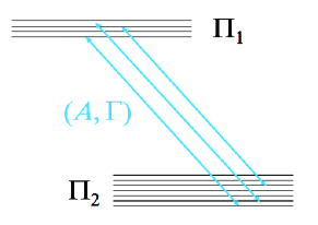
Figure 1: (Color online). Assumptions on the coupling scheme: the two subspaces $\Pi_{1}$ and $\Pi_{2}$ are connected through the operator $A$, but no transition is induced by $A$ within each subspace.

Two points are noteworthy: the complete positivity of the induced map (even considered the derivation beyond the secular approximation), and the independence of the dissipator from the specific form of $H_{\mathrm{S}}$. This second property is related to the fact that at a certain point we sum up over all the jump operators ($A(\omega)$), which ‘reconstructs’  the complete system operator involved in the system-bath interaction ($A$).

It is also interesting to sum up the hypotheses we have exploited. The first one is the typical weak coupling limit ($\gamma\rightarrow 0$) which is important to perform the Born approximation and start with the derivation of the master equation. The second hypothesis is the high temperature limit (which implies $N(\omega)\gg 1$) which allows to consider essentially equal the rates of the downward and upward transitions induced by the environment. The weak coupling limit makes even closer such rates, for any given frequency. Finally, the band structure for the energy spectrum of the system (also assuming that inter-band transitions are forbidden) and the narrowness of such bands ($\delta\omega/\omega_{0}\rightarrow 0$) allow to consider equal the rates for different frequencies, making it possible to reconstruct the operator $A$ from the relevant jump operators. These three different limits should be taken in such a way that $\gamma k_{B}T\delta\omega/(\hbar\omega_{0}^{2})\rightarrow 0$ (see Eq. (15)), which can be realized in many different ways. In particular, a weaker system-environment coupling or narrower bands allow to explore the thermal Zeno phenomenon at higher temperature.

3 Thermal Zeno Dynamics

General Statement — The structure of the master equation in Eq. (17) suggests the idea that under suitable hypotheses the dissipator can hinder some dynamical effects of $H_{\mathrm{S}}$, the free Hamiltonian of the system.

This statement can be proven through considerations similar to those made in previous works, in Hamiltonian contexts [2, 4] and in dissipative contexts [17]. Since $\alpha\equiv\gamma N(\omega_{0})$ is very large, we can treat the commutator $-i\left[H_{\mathrm{S}},\rho\right]$ as a perturbation with respect to the dissipator. Assuming this point of view, it is easy to convince oneself that the Hamiltonian cannot significantly connect subspaces of the dissipator which are well separated in terms of the relevant eigenvalues. In other words, assuming that $\rho_{\mathrm{a(b)}}$ is an eigenoperator of the dissipator associated to the eigenvalue $\alpha\lambda_{\mathrm{a(b)}}$ — this means that $2A\rho_{\mathrm{a(b)}}A-A^{2}\rho_{\mathrm{a(b)}}-\rho_{\mathrm{a(b)}}A^{2}=\lambda_{\mathrm{a(b)}}\rho_{\mathrm{a(b)}}$ — then, provided $\alpha|\lambda_{\mathrm{a}}-\lambda_{\mathrm{b}}|$ is much larger than the matrix elements of $H_{\mathrm{S}}$, the action of the commutator can only weakly connect the operators $\rho_{\mathrm{a}}$ and $\rho_{\mathrm{b}}$. Now, by increasing the temperature (and then $\alpha$) the eigenvalues and their differences increase, which makes more and more ineffective the free Hamiltonian $H_{\mathrm{S}}$ in determining transitions between different subspaces of the dissipator. The appearance of such constraints in the time evolution is just the signature of the (thermal) quantum Zeno effect, which gives rise to an inhibition of the time evolution if the initial state of the system belongs to a one-dimensional eigenspace of the dissipator, while gives rise to a Zeno dynamics (evolution in the restricted subspace) if the initial state belongs to a multiplet of the dissipator.

Three-state system in a high-Temperature reservoir — As a very special case, we analyze the following example of inhibition of the time evolution induced by temperature. Let us consider a three-state system governed by the following Hamiltonian:

$$H_{\mathrm{S}} =\sum_{l=1}^{3}\nu_{l}\left|l\right\rangle\left\langle l\right|+\left(\Omega\left|1\right\rangle\left\langle 2\right|+\mathrm{H.c.}\right)\,,$$ (18)

$$H_{\mathrm{B}} =\sum_{k}\omega_{k}a^{\dagger}_{k}a_{k}\,,$$ (19)

$$H_{\mathrm{I}} =\left(\left|2\right\rangle\left\langle 3\right|+\left|3\right\rangle\left\langle 2\right|\right)\otimes\sum_{k}g_{k}\left(a_{k}+a_{k}^{\dagger}\right)\,.$$ (20)

This model, which is represented in Fig. 2, has similarities with those analyzed in [17] and [18]. Nevertheless, it differs from the former because in the present case the Hamiltonian is time independent, and it differs from the latter since here counter-rotating terms are included in the system-bath interaction.

On the basis of Eq.(17), at very high temperature we obtain,

$$\frac{\mathrm{d}\rho}{\mathrm{d}t}={\cal G}\rho\,,$$ (21)

with

$${\cal G}\rho\approx-i\left[H_{\mathrm{S}},\rho\right]+\alpha\left[(2A\,\rho\,A-A^{2}\,\rho-\rho\,A^{2})\right]\,,$$ (22)

$$A=\left|2\right\rangle\left\langle 3\right|+\left|3\right\rangle\left\langle 2\right|\,.$$ (23)

This master equation has been obtained under the previous assumptions, i.e., high-temperature, band structure and intra-band transitions forbidden.

The matrix representation of the superoperator ${\cal G}$ is the following:

$${\cal G}=$$

$$\hskip-71.13188pt\left(\begin{array}[]{ccccccccc}0&\mathrm{i}\Omega^{*}&0&-\mathrm{i}\Omega&0&0&0&0&0\\ \mathrm{i}\Omega&-\alpha-\mathrm{i}\omega_{12}&0&0&-\mathrm{i}\Omega&0&0&0&0\\ 0&0&-\alpha-\mathrm{i}\omega_{13}&0&0&0&0&0&0\\ -\mathrm{i}\Omega^{*}&0&0&-\alpha-\mathrm{i}\omega_{21}&\mathrm{i}\Omega^{*}&0&0&0&0\\ 0&-\mathrm{i}\Omega^{*}&0&\mathrm{i}\Omega&-2\alpha&0&0&0&2\alpha\\ 0&0&0&0&0&-2\alpha-\mathrm{i}\omega_{23}&0&2\alpha&0\\ 0&0&0&0&0&0&-\alpha-\mathrm{i}\omega_{31}&0&0\\ 0&0&0&0&0&2\alpha&0&-2\alpha-\mathrm{i}\omega_{32}&0\\ 0&0&0&0&2\alpha&0&0&0&-2\alpha\\ \end{array}\right)\,,$$ (33)

where we have assumed the ordering $(\rho_{11},\rho_{12},\rho_{13},\rho_{21},\rho_{22},\rho_{23},\rho_{31},\rho_{32},\rho_{33})$, and exploited the notation $\omega_{ij}=\nu_{i}-\nu_{j}$.

The structure of this matrix is very similar to that we have found in Ref [17]. On the basis of the analysis developed therein, one easily deduces that for very large $\alpha$ a Zeno Phenomenon occurs. In fact, in the $\alpha\rightarrow\infty$ limit (to better visualize this situation, consider the complementary situation in which all the other quantities tends toward zero), the state $\left|1\right\rangle\left\langle 1\right|$ turns out to be very close to an eigenvector of ${\cal G}$ and therefore its survival probability approaches unity at every time: the higher $\alpha$, the closer to unity is the survival probability of $\left|1\right\rangle\left\langle 1\right|$ at every time.

This is in line with the results in [17], where no secular approximation has been made, and generalizes the results of [18], where counter-rotating terms are removed from the beginning in the interaction.

To reach the limit of very large $\alpha$, one needs a very high temperature compared to $\omega_{0}$, meaning that the thermal energy is supposed to be much larger than all the transition frequencies, i.e., $\alpha\gg\omega_{13},\omega_{23}$ (both $\sim\omega_{0}$) and, a fortiori, $\alpha\gg\omega_{12}$. Also $\alpha\gg\Omega$ must be satisfied.

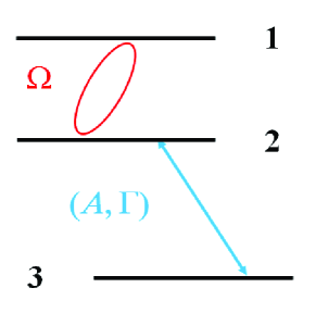
Figure 2: (Color online). Coupling scheme of the considered special case: states $1$ and $2$ are coupled by some external field; $2$ and $3$ are coupled by the environment. The subspace $\Pi_{1}$ is generated by $\left|1\right\rangle$ and $\left|2\right\rangle$, while $\Pi_{2}$ coincides with $\left|3\right\rangle$

.

4 Conclusions

In this paper we have presented a derivation of Markovian master equations beyond the secular approximation which is valid for a class of physical systems satisfying suitable hypotheses . In particular, it is important that the energy levels of the system form two bands and that the allowed transitions induced by the interaction with the bath are only between states of different bands.

The structure of the master equation obtained exhibits some important properties. First of all, it generates a completely positive map, in spite of the fact that it is derived beyond the secular approximation. Second, the structure of the dissipator is independent from the Hamiltonian associated to the small system and depends only on the operators involved in the system-bath interaction. This is a consequence of the first property, since summing up over all the jump operators associated to Bohr frequencies of the system restores the complete form of the system operator involved in system-bath coupling. Finally, on the basis of the structure of the master equation it is easy to forecast the incoming of Zeno phenomena at high temperature, which supports the results obtained in some previous works.

5 Acknowledgements

MS acknowledges financial support from the EPSRC grant EP/J014664/1.

References

- [1] Misra B and Sudarshan E C G 1997 J. Math. Phys. 18 7456
- [2] Facchi P, Lidar D A and Pascazio S 2004 Phys. Rev. A 69 032314
- [3] Facchi P and Pascazio S 2008 J. Phys. A: Math. Theor. 41 493001
- [4] Facchi P, Marmo G and Pascazio S 2009 J. Phys.: Conf. Ser. 196 012017
- [5] Home D and Whitaker M A B 1997 Ann. Phys. 258 237
- [6] Schulman L S 1998 Phys. Rev. A 57 1509
- [7] Panov A D 1999 Phys. Lett. A 260 441
- [8] Audretsch J, Mensky M B, Panov A D 1999 Phys.Lett. A 261 44
-
[9]
Keisuke Fujii and Katsuji Yamamoto 2010 Phys. Rev. A 82 042109; Gonzalo Alvarez, Bhaktavatsala Rao D D, Frydman L, and
Kurizki G 2010 Phys. Rev. Lett. 105 160401;
Schützhold R and Gnanapragasam G 2010 Phys. Rev. A 82 022120 - [10] Itano W M, Heinzen D J, Bollinger J J and Wineland D J 1990 Phys. Rev. A 41 2295.
- [11] Wilkinson S R, Bharucha C F, Fischer M C, Madison K W, MorrowP R, Qian Niu, Bala Sundaram, and Raizen M G 1997 Nature 387 575
- [12] Fischer M C, Gutiérrez-Medina B, and Raizen M G 2001 Phys. Rev. Lett. 87 040402
- [13] Kofman A G and Kurizki G 2001 Phys. Rev. Lett. 87 270405
- [14] Kavan Modi and Anil Shaji 2007 Phys. Lett. A 368 215
- [15] Maniscalco S, Piilo J and Suominen K-A 2006 Phys. Rev. Lett. 97, 130402
- [16] Ruseckas J 2002 Phys. Rev. A 66 012105
- [17] Scala M, Militello B, Messina A, and Vitanov N V 2011 Phys. Rev. A 84 023416
-
[18]
Militello B, Scala M, and
Messina A 2011 Phys. Rev. A 84 022106;
Militello B 2012 Phys. Rev. A 85 064102 -
[19]
Gorini V, Kossakowski A, and
Sudarshan E C G 1976 J. Math. Phys. 17 821-825;
Lindblad G, 1976 Commun. Math. Phys. 48 119 -
[20]
See for example: Crisp M D 1991 Phys. Rev. A 43
2430;
Aniello P, Porzio A and Solimeno S 2003 J. Opt. B: Quantum Semiclass. Opt. 5 S233;
Majenz C, Albash T, Breuer H-P and Lidar D 2013 Phyis. Rev. A 88 012103 - [21] C. W. Gardiner and P. Zoller 2000 Quantum Noise (Springer-Verlag, Berlin).
- [22] H.-P. Breuer and F. Petruccione 2002 The Theory of Open Quantum Systems (Oxford University Press, Oxford).