The Quadratic Coefficient of the Electron Cloud Mapping

Abstract

The Electron Cloud is an undesirable physical phenomenon which might produce single and multi-bunch instability, tune shift, increase of pressure ultimately limiting the performance of particle accelerators. We report our results on the analytical study of the electron dynamics.

1 INTRODUCTION

The electron cloud develops quickly as photons, striking the vacuum chamber wall, knock out electrons which are subsequently accelerated by the beam and strike the chamber again, producing further electrons in an avalanche process. Most studies [1] performed so far were based on computer simulations (e.g. ECLOUD [2]) taking into account photoelectron production, secondary electron emission, electron dynamics, and space charge effects, and providing a very detailed description of the electron cloud evolution. In [3] it was shown that, for the typical parameters of the Relativistic Heavy Ion Collider (RHIC), the evolution of the longitudinal electron cloud density evolution from bunch to bunch can be described (locally, i.e., at an arbitrary chosen point along the beam path) specific by a simple ”cubic map” of the form:

$$\rho_{m+1}\,=\,\alpha\,\rho_{m}+\beta\,{\rho_{m}}^{2}+\gamma\,{\rho_{m}}^{3}$$ (1)

where $\rho_{m}$ is the average electron cloud density after the $m$-th passage of the bunch. A similar map was next suggested and found to be reliable also for the Large Hadron Collider (LHC) [5]. The coefficients $\alpha$, $\beta$, $\gamma$ are extrapolated from simulations, and are functions of the beam parameters and of the beam pipe features. The linear term describes the linear growth and the coefficient $\alpha$ is larger than unity in the presence of electron cloud formation. The quadratic term describes the space charge effects, and is negative reflecting the concavity to the curve $\rho_{m+1}$ vs $\rho_{m}$. The cubic term corresponds to a variety of subtler effects, acting as perturbations to the above simple scenario.

From Figure 1 one can see that the bunch-to-bunch evolution contains enough informations about the build-up or the decay time, although the details of the line electron density oscillation between two bunches are lost. The average longitudinal electron density as function of time grows exponentially until the space charge due to the electrons themselves produces a saturation level. Once the saturation level is reached the average electron density does not change significantly. The final decay corresponds to the empty interval between successive bunches.

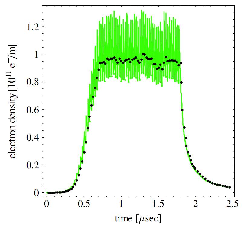
Figure 1: Time evolution of the electron density (green line) computed with ECLOUD. The black dots mark the average electron density between two consecutive bunches obtained with the map formalism. The machine/beam parameters used are listed in Table 1.

Fig. 2 shows the behavior of the average electron density $\rho_{m+1}$ as function of the average electron density $\rho_{m}$ for different values of the bunch population (number of particles in a bunch, $N_{b}$).

Figure 2: Average longitudinal electron density for different bunch populations (green: $N_{b}\,=\,8*10^{10}$, blue: $N_{b}\,=\,16*10^{10}$). The lines correspond to cubic fits. The red line corresponds to the identity map $\rho_{m+1}\,=\,\rho_{m}$. By comparison with Fig. 1, points above this line describe the initial growth and saturation of the bunch-to-bunch evolution of the electron density, those below describe the decay. The black line represents the cubic fit of the points corresponding to the first empty bunches.

Parameter	Quantity	Unit	Value
Beam pipe radius	$b$	m	$.045$
Beam size	$a$	m	$.002$
Bunch spacing	$s_{b}$	m	$1.2$
Bunch length	$h$	m	$.013$
Particles per bunch	$N_{b}$	$10^{10}$	$4\,\div\,9$

Table 1: Input parameters for analytical estimate and ECLOUD simulations.

The markers in Fig. 2 were obtained from ECLOUD; the lines are the cubic fits among these points.

The electron cloud dynamics can be roughly described as follows: starting with a small initial linear electron density, after some bunches the density takes off and reaches the corresponding saturation line ($\rho_{m+1}\,=\,\rho_{m}$, red line) where the space charge effects, due to the electrons in the cloud itself, take place. In this situation, points corresponding to successive passages of filled bunches, are in the same spot.

Until recently, the map coefficients have been extrapolated from simulations, in a purely empirical way, so as to obtain the best fit. An analytical expression of the linear coefficient $\alpha$ has been computed in a drift space [3], and in the presence of a magnetic dipole field [5].

In this paper we summarize our recent results [6] on the calculation of an analytical expression for the quadratic coefficient $\beta$ in Eq. (1), under the simple assumptions of round chambers and free-field motion of the electrons in the cloud. The coefficient $\beta$ turns out to depend on few beam and machine parameters, and can be computed analytically once and for all, saving a huge computational time compared to numerical simulations obtained using ECLOUD [1].

This paper is accordingly organized as follows. In the next section we calculate the saturation density of cloud electrons, adopting a gaussian-like distribution for the secondary electrons, producing an energy barrier near the chamber wall. Later we deduce the formula for the linear coefficient $\alpha$, already given in [4], and also for the quadratic coefficient, which is a new result. Finally we report the conclusions.

2 CLOUD SATURATION DENSITY

Electrons in the cloud include both primary electrons, generated by synchrotron radiation at the pipe wall, and secondary electrons, produced by beam induced multi-pactoring. Primary electrons interact with the parent bunch, and are accelerated to a velocity $v_{p}\!=\!2c\bar{N}_{b}r_{e}/b$, $r_{e}$ being the classical electron radius, $b$ the pipe radius, and $\bar{N}_{b}$ the linear particle density of a longitudinally-uniform (coasting) beam having the same total charge as the actual bunched beam,

$$\bar{N}_{b}\,=\,\frac{h}{h+s_{b}}N_{b}$$ (2)

with $s_{b}$ the intra-bunch spacing, and $h$ the bunch length.

Secondary electrons are produced with a low (typically a few $eV$) energy ${\mathcal{E}}_{0}$, and move from the pipe wall, with velocity $v_{s}\,=\,c\,\sqrt{2{\mathcal{E}}_{0}/mc^{2}}$ until the next bunch arrives. For large $N_{b}$, $v_{s}<v_{p}$. Cloud buildup turns out to depend basically on two parameters [7]:

$$k=\frac{2\bar{N}_{b}r_{e}h}{b^{2}}=b^{-1}v_{p}\frac{h}{c},$$ (3)

and

$$\xi=\frac{h}{b}\sqrt{\frac{2{\mathcal{E}}_{0}}{mc^{2}}}=b^{-1}v_{s}\frac{h}{c},$$ (4)

The parameters $k$ and $\xi$ are measures of the distances (in units of the pipe radius $b$) traveled, respectively, by primary and secondary electrons during the bunch transit time. At low currents, $k\!\ll\!1$, primary electrons interact with several bunches before eventually reaching the wall. In the opposite extreme case, $k\!>\!2$, they travel from wall to wall in a single bunch transit-time. The transition between the two regimes can be expected to occur at $k\!\sim\!1$.

For $k\!\!>\!\!1$ secondary electrons are confined in a layer $\xi\!<\!r/b\!<\!1$ near the pipe wall, and are wiped out of the region $0\!<\!r/b\!<\!\xi$ close to the beam by each passing bunch. Operating in the range of parameters ($k\!>\!1$ and $2-k\!<\!\xi\!<1$) is thus clearly desirable to suppress the adverse effects of the e-cloud on the beam dynamics [7]. In this range secondary electrons create a space-charge energy barrier near the wall, where they are locked up, and their density grows until this barrier exceeds their native energy ${\mathcal{E}}_{0}$, viz.

$$-e\,V(1-\xi)\,\geq\,{\mathcal{E}}_{0}$$ (5)

where $V$ is the electric potential generated by the electron cloud, and $-e$ is the electron charge. The saturation condition corresponds to the equality in eq. (5).

To compute the potential in (5) we assume a Gaussian radial dependence for the electron cloud charge density, peaked at $r_{0}$, with std. deviation $\sigma$, viz.

$$\rho(r)\,=\,\rho_{0}\exp\left[-\frac{(r-r_{0})^{2}}{2\sigma^{2}}\right],$$ (6)

where $\rho_{0}$ is fixed by the condition

$$2\pi h\int_{a}^{b}\rho(r)rdr\,=\,-N\,e$$ (7)

$N$ being the total number of electrons in the cylindrical shell with radii $a,b$ and height $h$ around each bunch. Introducing the dimensionless quantities $\tilde{a}=a/b$, $\tilde{r}=r/b$, $\tilde{r}_{0}=r_{0}/b$, $\tilde{\sigma}=\sigma/b$, $g=\bar{N}_{b}/N$ and $V_{0}=Ne/2\pi\epsilon_{0}h$, the (total) electric field and potential in the beam pipe can be written:

$$\mathbf{E}(\tilde{r})\,=\,V_{0}\left[g-\frac{F(\tilde{r})}{F(1)}\right]\frac{\hat{\mathbf{r}}}{r},$$ (8)

$$V(\tilde{r})\,=\,-V_{0}\left[g\ln\tilde{r}+\frac{G(\tilde{r})}{F(1)}\right]$$ (9)

where

$$F(\tilde{r})=\int_{\tilde{a}}^{\tilde{r}}\exp\left[-\frac{(y-\tilde{r}_{0})^{2}}{2\tilde{\sigma}^{2}}\right]y\,dy=$$ (10)

and

$$G(\tilde{r})=\int_{\tilde{r}}^{1}\,\frac{F(y)}{y}dy,$$ (11)

The limiting form of the potential for $\tilde{\sigma}\!\gg\!1$ (i.e., for a uniform cloud charge density), and $\tilde{a}\,\rightarrow\,0$ (vanishingly thin beam) is:

$$V\rightarrow-V_{0}\biggl{[}g\ln\tilde{r}+\frac{1-\tilde{r}^{2}}{2}\biggr{]}.$$ (12)

Figure 3 displays the potential (9) as a function of $\tilde{r}$, for various values of $g$. The limiting form (12) is also shown for comparison (dashed lines). The potential (12) is minimum at $\tilde{r}\,=\,\tilde{r}_{m}\,=\sqrt{g}$. For $g\!>\!1$ it decreases monotonically with $\tilde{r}$ throughout the beam pipe $(0\!\leq\!\tilde{r}\!\leq\!1)$. The condition $g\,=\,1$ corresponding to $N=N_{b}$, i.e., to the well known condition of neutrality [7]. The potential (9) obtained from the Gaussian cloud density profile (6) behaves similarly.

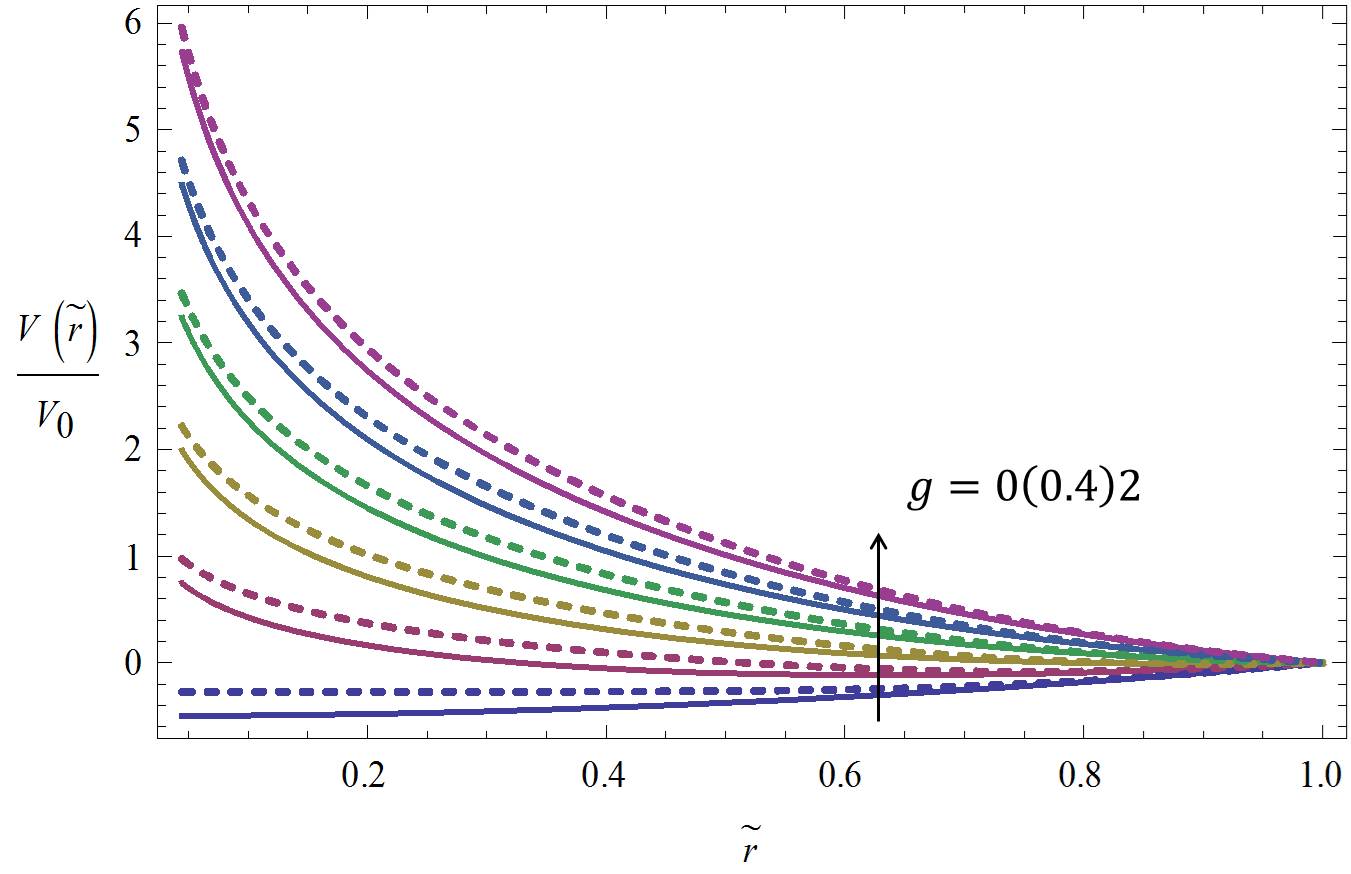
Figure 3: The potentials in Eq. (9) (dashed lines), and (12) (solid lines) as functions of $\tilde{r}$ for various values of $g$ and $\tilde{a}\!=\!0.04$, $\tilde{r}_{0}\!=\!0.8$, $\tilde{\sigma}\!=\!0.2$.

The space-charge energy barrier ${\mathcal{E}}(r)\,=\,-e\,V(r)$ faced by the electrons originated at the walls is compared in Figure (4) to the the electron density $n(\tilde{r})=-\rho(\tilde{r})/e$.

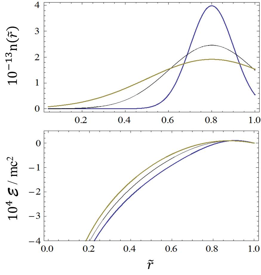
Figure 4: The electron density $n(\tilde{r})$ (solid line) and the energy barrier ${\mathcal{E}}(\tilde{r})$ (dashed line) for $\tilde{\sigma}\,=\,0.1(0.1)0.3$, $\tilde{r}_{0}\,=\,0.8$, $N_{b}\,=\,6\cdot 10^{1}0$.

It is seen that the position of the peak of the energy barrier corresponds to the maximum concentration of the electrons, and the barrier height goes to zero where the electron density vanishes. The saturation condition eq.(5) yields the following critical number of electrons in the cloud

$$N_{sat}\,=\,\frac{F(1)}{G(1-\xi)}\left[\frac{{\mathcal{E}}_{0}\,h}{2m\,c^{2}\,r_{e}}-\bar{N}_{b}\ln(1-\xi)\right]$$ (13)

where $r_{e}$ is the classical radius of electron. Assuming the electrons as confined in a cylindrical shell with inner radius $r_{0}-3\sigma$ and external radius $b$ the average saturation density can be written as

$$n_{sat}\,=\,\frac{\rho_{sat}}{-e}\,=\,\frac{N_{sat}}{\pi hb^{2}[1-(\tilde{r}_{0}-3\tilde{\sigma})^{2}]},$$ (14)

If the electrons are uniformly distributed in the region $a\!\leq\!r\!\leq b$ we get

$$\bar{n}_{sat}\,=\,\frac{\bar{\rho}_{sat}}{-e}\,=\,\frac{\bar{N}_{sat}}{\pi hb^{2}[1-\tilde{a}^{2}]}.$$ (15)

In Figure 5 we show the behavior of the saturation densities (14) and (15).

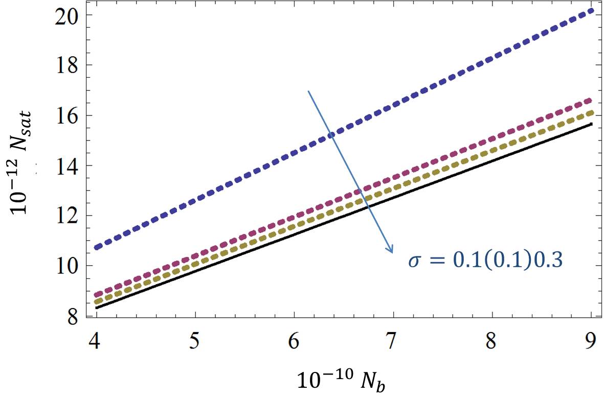
Figure 5: The saturation electron density vs $N_{b}$. Equation (15) (solid line) and eq. (14) (dashed lines) for $\tilde{\sigma}\,=\,0.1(0.1)0.3$, with $\tilde{a}\,=\,0.04$, $\tilde{r}_{0}\,=\,0.8$.

3 ANALYTICAL DETERMINATION of COEFFICIENTS

Let $N_{m}$ the total number of electrons in the cloud at the passage of bunch-$m$. After the passage of the bunch they are brought to an energy

$${\mathcal{E}}_{g}\,=\,m_{e}c^{2}\frac{r_{e}N_{b}}{\sqrt{2\pi}h}\left[\log\biggl{(}\frac{b}{1.05a}\biggr{)}-\frac{1}{2}\right]$$ (16)

(see [8] for derivation). After a first collision with the pipe wall, two electron jets are created: a reflected (back-scattered) one, containing of $\delta_{r}({\mathcal{E}}_{g})N_{m}$ electrons, with energy ${\mathcal{E}}_{g}$, and a ”true” secondary one, containing $\delta_{t}({\mathcal{E}}_{g})N_{m}$ electrons, with energy ${\mathcal{E}}_{0}$. The quantities $\delta_{r,s}$ are referred to as $SEY$ (Secondary Emission Yield) [9]), and the process proceeds in cascade until the next bunch arrives, as sketched in Figure 6.

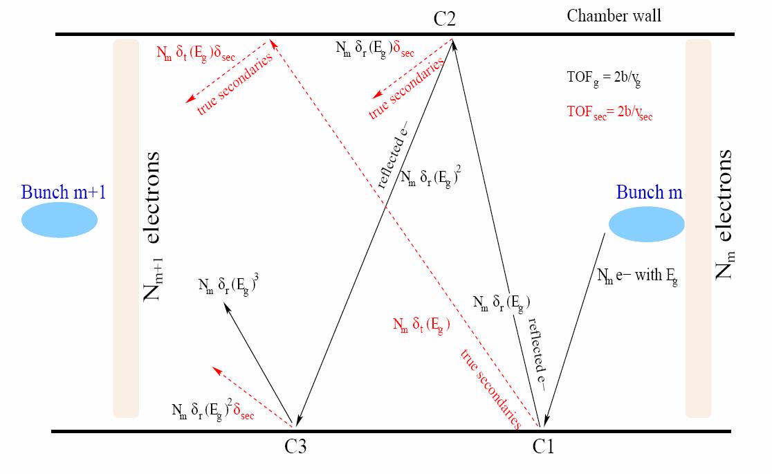
Figure 6: Sketch of the electron cloud evolution in the time interval between two successive bunches. The $m$-th bunch accelerates the $N_{m}$ electrons towards the chamber wall with energy ${\mathcal{E}}_{g}$. The first collision (C1) at the wall producwa two jets: the first one consisting of $N_{m}\delta_{r}$ backscattered electrons (black line), with energy ${\mathcal{E}}_{g}$; the second one consisting of $N_{m}\delta_{t}$ secondary electrons (red dotted line) with low energy . Before the $(m+1)$-th bunch arrives, these two jets undergo further collisions, originating further jets. The sum of over all these jets gives $N_{m+1}$

During the interval $t_{sb}=h/\beta c$ preceding the passage of the next bunch, electrons with ${\mathcal{E}}\!=\!{\mathcal{E}}_{g}$ undergo a total number of collisions with the pipe wall given by

$$S\,=\,\frac{t_{sb}-t_{f}({\mathcal{E}}_{g})}{t_{f}({\mathcal{E}}_{g})},$$ (17)

where $t_{f}({\mathcal{E}_{g}})$ is the wall-to-wall flight time for an electron with energy ${\mathcal{E}_{g}}$ (averaged over all possible angles w.r.t. to the pipe axis), obtained from

$$t_{f}({\mathcal{E}})\,=\,\frac{4b}{\pi\sqrt{2{\mathcal{E}}/m_{e}}}$$ (18)

Hence the total numer of high-energy electrons at the arrival of bunch-$(m\!+\!1)$ is

$$N_{m+1}({\mathcal{E}}_{g})\!=\!N_{m}\delta^{S}_{r}({\mathcal{E}}_{g}).$$ (19)

The jet of low-energy secondary electrons originating after the $p-th$ collision of the high energy electrons contains

$$\delta_{s}({\mathcal{E}}_{g})\delta_{r}^{p-1}({\mathcal{E}}_{g})N_{m}$$

electrons with energy ${\mathcal{E}}_{0}$. These low energy electrons, will undergo a further number of collisions with the walls, before the next bunch arrives, given by

$$k_{p}=\frac{t_{sb}-p\mbox{}t_{f}({\mathcal{E}}_{g})}{t_{f}({\mathcal{E}}_{0})}$$ (20)

and at each collisions the number of these (slow) electrons will change by a factor $\delta_{r}({\mathcal{E}}_{0})\!+\!\delta_{r}({\mathcal{E}}_{0})$, since both the reflected and secondary electrons will have the same energy ${\mathcal{E}}_{0}$. The total number of low-energy electrons at the arrival of bunch-$(m+1)$ will accordingly be

$$N_{m\!+\!1}({\mathcal{E}}_{0})\!=\!N_{m}\delta_{s}({\mathcal{E}}_{g})\cdot$$

$$\cdot\sum_{p=1}^{S}\delta^{p-1}_{r}({\mathcal{E}}_{g})\left[\delta_{t}({\mathcal{E}}_{0})\!+\!\delta_{r}({\mathcal{E}}_{0})\right]^{k_{p}}$$ (21)

The number of (fast and slow) electrons $N_{m+1}$ on the arrival of bunch-$(m+1)$ is thus given by:

$$N_{m+1}\,=\,N_{m}\left[{\delta_{r}}^{S}({\mathcal{E}}_{g})\!+\!\delta_{t}({\mathcal{E}}_{g})\right.\cdot$$

$$\cdot\left.\sum_{p=1}^{S}{\delta_{r}}^{p-1}({\mathcal{E}}_{0}){\delta_{tot}^{k_{p}}({\mathcal{E}}_{0})}\right]$$ (22)

having set $\delta_{tot}=\delta_{r}+\delta_{s}$. The above argument ignores saturation effects, and can be consistently used to express the linear coefficient in the cubic map (1) in terms of the SEY coefficients, whose dependence from energy is known [9], as follows

$$\alpha\!=\!\frac{N_{m+1}}{N_{m}}\!=\!\delta_{r}^{S}({\mathcal{E}}_{g})+$$

$$+\delta_{t}({\mathcal{E}}_{g})\delta_{tot}^{\eta}({\mathcal{E}}_{0})\frac{\delta_{tot}^{\eta S}({\mathcal{E}}_{0})\!-\!\delta_{r}^{S}({\mathcal{E}}_{0})}{\delta_{tot}^{\eta}({\mathcal{E}}_{0})\!-\!\delta_{r}({\mathcal{E}}_{0})}$$ (23)

where $\eta=t_{f}({\mathcal{E}}_{g})/t_{f}({\mathcal{E}}_{0})=({\mathcal{E}}_{0}/{\mathcal{E}}_{g})^{1/2}\ll 1$.

The coefficient $\beta$ in the cubic map (1) can now be found by considering the saturation condition, where

$$n_{sat}\,=\,\alpha\,n_{sat}+\beta\,{n_{sat}}^{2}\,\,\,\,$$ (24)

yielding

$$\beta\,=\,\frac{1-\alpha}{n_{sat}}$$ (25)

Note that as ${\mathcal{E}}_{g}\rightarrow\infty$, the quantity $S$ diverges, according to (17), and hence the contribution of the high-energy electrons to eq. (22) becomes negligible, given that $\delta_{r}(\infty)<1$ [9]. We may accordingly use the saturation density of the secondary electrons, derived in Section 2, to evaluate the quadratic coefficient via (25). In Figure (7) we compare our analytic result for $\beta$ to the outcomes of simulations (ECLOUD code) using the parameters in Table 1. A good qualitative agreement is obtained, for the assumed Gaussian charge distribution.

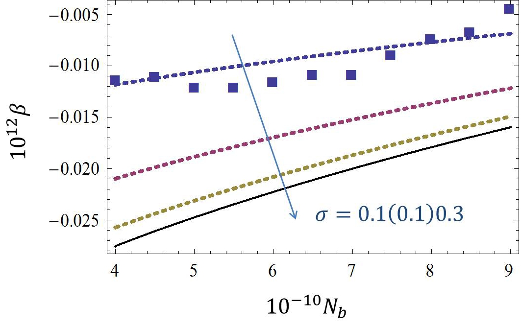
Figure 7: The quadratic coefficient $\beta$ Eq. (24) versus $N_{b}$ (dashed lines), for $\tilde{\sigma}=0.1(0.1)0.3$ and $\tilde{r}_{0}=0.95$, and the corresponding values from ECLOUD simulations (markers). The solid line is obtained using in (25), the uniform electron density (15) .

4 CONCLUSIONS

The main results in this paper can be summarized as follows. A simple analytic form for the quadratic map coefficient $\beta$ has been derived, and found to be in good agreement compared to results obtained from ECLOUD simulations. The map formalism can thus be easily applied to determine safe regions in parameter space where the accelerator can be operated without suffering from problems originated by the electron clouds.

References

- [1] F. Zimmermann, ”A Simulation Study of Electron-Cloud Instability and Beam-Induced Multipacting in the LHC,” CERN LHC-Project-Rept. 95 (1997).
- [2] http://ab-abp-rlc.web.cern.ch/ab-abp-rlc-ecloud/.
- [3] U. Iriso, S. Peggs, ”Maps for Electron Clouds,” Phys. Rev. ST-AB 8 (2005) 024403.
- [4] U. Iriso, S. Pegg., ”An Analytic Calculation of the Electron Cloud Linear Map Coefficient,” Proc. EPAC ’06, Edinburgh (UK), June 26-30 2006, paper MOPCH133.
- [5] Th. Demma et al., ”Maps for Electron Cloud Density in Large Hadron Collider Dipoles,” Phys. Rev. ST-AB 10 (2007) 114401.
- [6] Th. Demma et al., ”E-Cloud Map Formalism: an Analytical Expression for Quadratic Coefficient,” Proc. IPAC’10, Kyoto (JP), May 23-28 2010, paper TUPD037.
- [7] S. Heifets, ”Electron Cloud at High Beam Currents,” SLAC-PUB-9584 (2002).
- [8] S. Berg, ”Energy Gain in an Electron Cloud following the Passage of a Bunch,” CERN LHC Proj. Note 97 (1997).
- [9] M. Furman, M. Pivi, ”Probabilistic Model for the Simulation of Secondary Electron Emission,” Phys. Rev. ST-AB 5 (2002) 12404.