Graphical Calculus for the Double Affine
$Q$-Dependent Braid Group

Abstract

We define a double affine $Q$-dependent braid group. This group is constructed by appending to the braid group a set of operators $Q_{i}$, before extending it to an affine $Q$-dependent braid group. We show specifically that the elliptic braid group and the double affine Hecke algebra (DAHA) can be obtained as quotient groups. Complementing this we present a pictorial representation of the double affine $Q$-dependent braid group based on ribbons living in a toroid. We show that in this pictorial representation we can fully describe any DAHA. Specifically, we graphically describe the parameter $q$ upon which this algebra is dependent and show that in this particular representation $q$ corresponds to a twist in the ribbon.

1 Introduction

Representation theory is an essential tool in mathematical and physical research. To this end, linear algebra, the theory of special functions, arithmetic and related combinatorics are its usual objectives. A particularly potent example illustrating the power of representation theory may be offered in the context of Hecke-type algebras [1].

In this paper we define a Hecke-type structure called the double affine $Q$-dependent braid group and investigate its properties. Among its quotient groups is the double affine Hecke algebra (DAHA) which is of particular interest as its polynomial representations [2] have close connections to Macdonald and Jack polynomials [3]. Furthermore, we have seen how some specific polynomials emerging from this algebra, when subject to special wheel conditions, yield interesting $q$-deformed Laughlin and Haldane-Rezayi wave functions [4, 5]. These are believed to be excellent candidates for describing quantum Hall effect ground states; by adjusting the wheel condition parameters, one may fix the filling fraction of these wavefunctions. Other polynomials directly obtained from the DAHA can, in a similar fashion, be used to describe the ground states of $O(n)$ models [6].

We provide an intuitive pictorial representation of a DAHA in this paper. It is difficult to overestimate the power of graphical representations in illustrating abstract concepts in pure mathematics. Since the emergence of the intuitive pictorial representation of the braid group there has been a massive interest in its structure, greatly advancing the field. For example, when Kauffman introduced diagrams [7] to explain the Jones polynomial [8] in the context of Hecke algebras, the subject became more accessible and widely-known.

Before presenting our graphical representation which provides an interpretation of all DAHAs and their underlying parameters, we firstly establish the relation of DAHAs to other well known abstract algebraic structures. In particular we define and give readers a clear picture of the structure of a double affine $Q$-dependent braid group ($\mathcal{D}_{N}\{Q\}$). It is constructed by appending to the braid group a set of $N$ operators $\{Q_{i}\}=\{Q_{1}\ldots,Q_{N}\}$, before extending it to an affine $Q$-dependent braid group.

Our interest in $\mathcal{D}_{N}\{Q\}$ stems from its pole position with respect to other algebraic structures whose primary element is a braid group. In fact, appending to the double affine braid group a set of operators $\{Q_{i}\}$ generalises the underlying braid group. It does so by turning braid group strands into ribbons and permitting $2\pi$ twists. The original braid group then corresponds to $\mathcal{B}_{N}\{Q\}/\langle Q_{i}\rangle$, where $\langle Q_{i}\rangle$ is freely generated by the operators $Q_{i}$. Thus the original braid group is in other words equivalent to $\mathcal{B}_{N}\{Q\}$ where $Q=1$. Similarly the affine braid group corresponds to $\mathcal{A}_{N}\{Q\}/\langle Q_{i}\rangle$. Naturally the elliptic braid group [9, 10] is obtained from $\mathcal{D}_{N}\{Q\}$ by ignoring the twists or equivalently by contracting ribbons to strands, i.e. $\mathcal{D}_{N}\{Q\}/\langle Q_{i}\rangle$. In addition, taking the quotient $\mathcal{D}_{N}\{Q\}/\langle Q_{i}Q_{i+1}^{-1}\rangle$ is equivalent to considering twists on different ribbons as identical. Furthermore imposing the Hecke relation and setting $Q_{i}=q\mathbb{1}$, where $q\in\mathbb{C}$, we obtain the double affine Hecke algebra (of type A) [1, 11]. These relations are illustrated in Figure 1. Note that $\mathcal{B}_{N}\{Q\}=\mathcal{B}_{N}(Q_{1},Q_{2},\ldots,Q_{N})$ and $\mathcal{B}_{N}(Q)=\mathcal{B}_{N}\{Q\}/\langle Q_{i}Q_{i+1}^{-1}\rangle\simeq\mathcal{B}_{N}(Q,Q,\ldots,Q)$.

Figure 1: Commutative diagram describing the relations of $\mathcal{D}_{N}\{Q\}$ with other algebraic structures whose primary element is a braid group.

Complementing the algebraic description of a double affine $Q$-dependent braid group, we provide a pictorial representation. The graphical calculus is based on ribbons within cubes, where opposite vertical faces of the cube are identified; a topologically equivalent presentation is given in terms of ribbons living inside a toroid. We clearly illustrate all of the defining relations of $\mathcal{D}_{N}\{Q\}$ in our new cube-ribbon representation. It provides a concrete visual description of its structure, in particular we obtain a very straightforward interpretation of the action of the generators $Q_{i}$ who create $2\pi$ twists in the ribbons. In the quotient group $\mathcal{D}_{N}\{Q\}/\langle Q_{i}Q_{i+1}^{-1}\rangle$, where we obtain the double affine Hecke algebra, we show that $q$ corresponds to the factor when replacing a ribbon with a twist by one with no twist at all. Hence our cube-ribbon representation describes double affine Hecke algebras for all values of $q$. In $\mathcal{D}_{N}\{Q\}/\langle Q_{i}\rangle$ the ribbons are reduced to strands and twists are no longer possible, therefore our pictorial representation gives a toroidal description of the elliptic braid group.

The layout of this paper is as follows: in Sections 1 through 3, we define the $Q$-dependent braid group and introduce the affine $Q$-dependent braid group. We give their defining relations – which depend on a set of operators $\{Q_{i}\}$ – and pictorially represent their generators.

In Section 4 we present the complete construction of the double affine $Q$-dependent braid group. We outline our method of graphically representing this group structure, which depends on the set of $\{Q_{i}\}$ and obtain the main result of this paper: that is we show that each generator $Q_{i}$ creates a twist in the ribbon. We also show that when $\{Q\}=1$ our cube-ribbon representation describes the elliptic braid group.

In Section 5 we indicate how to obtain the double affine Hecke algebra from $\mathcal{D}_{N}\{Q\}$. We highlight that our graphical calculus is valid for all DAHAs, with no restriction on the parameter $q$ upon which this algebra depends.
Finally we conclude with some discussion as to how this pictorial representation could settle some unresolved issues, specifically regarding matrix and tangle representations, and outline some related future work.

2 The Braid Group

Throughout this paper we follow the general approach of [4, 6], namely, we present all of the algebraic relations in terms of multiplication rules for the elements of the algebra. One could adopt a much more rigourous approach via group quotients, etc. as in [1, 12], but here we opt for this more “physics” approach.

2.1 The $Q$-Dependent Braid Group $\mathcal{B}_{N}\{Q\}$

We begin by reviewing the the braid group and its $Q$-dependent extension. These are essential to our construction of $\mathcal{D}_{N}\{Q\}$. Similarly its well-established pictorial representation serves as a starting point for our cube-ribbon representation.

The $N$-strand braid group $\mathcal{B}_{N}$ is as follows [13]: $\mathcal{B}_{N}$ is the group generated by the $N-1$ invertible elements $\{T_{i}|i=1,..,N-1\}$ satisfying the relations

$$T_{i}T_{j} = T_{j}T_{i}\mbox{ for }|i-j|\geq 2,$$ (2.1)

$$T_{i}T_{i+1}T_{i} = T_{i+1}T_{i}T_{i+1}\mbox{ otherwise }.$$ (2.2)

(The second of the above is referred to as the braid relation.)

It is indeed well known that this algebraic description can be incorporated into a pictorial one by defining $T_{i}$ and its inverse $T^{-1}_{i}$ to correspond to the exchange of the $i^{\mathrm{th}}$ and $(i+1)^{\mathrm{th}}$ strands as illustrated below:

Multiplication is then defined by stacking: AB is the braid obtained by stacking A on top of B and gluing the bottom ends of the strands in A to the top ends of those in B.

We now define the $N$-strand $Q$-dependent braid group, $\mathcal{B}_{N}\{Q\}$, as follows: $\mathcal{B}_{N}\{Q\}$ is the group generated by the invertible elements $\{T_{i}|i=1,..,N-1\}$ satisfying (2.1) and (2.2), in addition to a set of commuting elements $\{Q_{i}|i=1,..,N\}$ satisfying the relations

$$Q_{i}Q_{j} = Q_{j}Q_{i}\mbox{ for all }i,j,$$ (2.3)

$$T_{i}Q_{j} = Q_{j}T_{i}\mbox{ for }j<i,j>i+1,$$ (2.4)

$$T_{i}Q_{i} = Q_{i+1}T_{i}\mbox{ for }i=1,\ldots,N-1,$$ (2.5)

$$T_{i}Q_{i+1} = Q_{i}T_{i}\mbox{ for }i=1,\ldots,N-1.$$ (2.6)

These relations imply $T^{2}_{i}Q_{j}=Q_{j}T^{2}_{i}$ for all $i,j$, that is the $Q$s commute with all even powers of the $T$s but not with odd powers.

The above relations may be familiar to many readers. They appear in the study of framed, or ribbon, braid groups, introduced in [14]. A more in-depth and mathematically rigourous treatment of framed braids or ribbon braids can be found in [15, 16], among others. We use this well-known structure as a starting point for establishing the proper context for our treatment of DAHAs.

As it stands, only the trivial braids – those whose strands go straight from top to bottom without crossing – can represent the $Q$s in a way consistent with (2.3)-(2.6). We shall see later how to introduce nontrivial graphical representations for the $Q$s.

3 Affine Braid Groups

3.1 The Affine Braid Group $\mathcal{A}_{N}$

The $Q$-dependent braid group $\mathcal{B}_{N}\{Q\}$ can be extended to an affine braid group $\mathcal{A}_{N}$ by appending to it $N$ invertible operators $Y_{i}$. These satisfy the relations

$$Y_{i}Y_{j} = Y_{j}Y_{i}\mbox{ for all }i,j,$$ (3.1)

$$T_{i}Y_{j} = Y_{j}T_{i}\mbox{ for }j\neq i,i+1,$$ (3.2)

$$T_{i}Y_{i+1}T_{i} = Y_{i}\mbox{ for }i=1,\ldots,N-1.$$ (3.3)

The last of these relations implies that we need only one of the $Y_{i}$ (and all of the $T_{i}$) to generate the others. For example, (3.3) can be used to rewrite $Y_{i}$ for $i=2,\ldots,N$ as

$$Y_{i} = T^{-1}_{i-1}T^{-1}_{i-2}\ldots T^{-1}_{1}Y_{1}T^{-1}_{1}\ldots T^{-1}_{i-2}T^{-1}_{i-1}.$$

$\mathcal{A}_{N}$ is thus fully generated by $Y_{1}$ and the $T_{i}$.

A more elementary presentation [1, 6] is to write all the $Y_{i}$ in terms of $T_{i}$ and an element $\sigma$ defined as

$$\sigma := T^{-1}_{N-1}T^{-1}_{N-2}\ldots T^{-1}_{1}Y_{1}.$$ (3.4)

All of the $Y_{i}$ can now be written in terms of $\sigma$ and the $T_{i}$ using (3.3):

$$\qquad Y_{i} = \left\{\begin{array}[]{ll}T_{1}T_{2}\ldots T_{N-1}\sigma&i=1\,,\\ T_{i}\ldots T_{N-1}\sigma T^{-1}_{1}\ldots T^{-1}_{i-1}&i=2,\ldots,N-1,\\ \sigma T^{-1}_{1}\ldots T^{-1}_{N-1}&i=N.\end{array}\right.$$

The other defining relations for $\mathcal{A}_{N}$, (3.1) and (3.2), may be rewritten in terms of $\sigma$ as

$$T_{i-1}\sigma=\sigma T_{i}, i=2,\ldots,N-1,$$

$$T_{N-1}\sigma^{2}=\sigma^{2}T_{1}.$$

Also of interest is that the above relations imply that $\sigma^{N}T_{i}=T_{i}\sigma^{N}$. This tells us that $\sigma^{N}$ commutes with all the $Y_{i}$, and thus $\sigma^{N}$ is central in $\mathcal{A}_{N}$. We could then label irreducible representations of $\mathcal{A}_{N}$ with the eigenvalues of $\sigma^{N}$ if necessary.

3.2 The Affine $Q$-Dependent Braid Group $\mathcal{A}_{N}\{Q\}$

In a similar fashion to $\mathcal{B}_{N}\{Q\}$, we extend $\mathcal{A}_{N}$ to an affine $Q$-dependent braid group, $\mathcal{A}_{N}\{Q\}$, by defining how the set of elements $\{Q_{i}|i=1,..,N\}$ interact with the affine generators $Y_{i}$.

Therefore in addition to all of the defining relations of $\mathcal{A}_{N}$, the generators of $\mathcal{A}_{N}\{Q\}$ must also satisfy

$$Y_{i}Q_{j} = Q_{j}Y_{i}\mbox{ for all }i,j.$$ (3.6)

Using the definition of $\sigma$, (3.4), one can rewrite (3.6), to obtain $\mathcal{A}_{N}\{Q\}$ purely in terms of $T_{i}$, $\sigma$ and $Q_{i}$:

$$\sigma Q_{i} = Q_{i-1}\sigma\mbox{ for }i=2,\ldots,N,$$

$$\sigma Q_{1} = Q_{N}\sigma.$$

These relations also imply that $\sigma^{N}Q_{i}=Q_{i}\sigma^{N}$. Having fully described our definition of an affine $Q$-dependent braid group, $\mathcal{A}_{N}\{Q\}$, we now incorporate its algebraic structure into an intuitive graphical one.

3.3 Pictorially Representing $\mathcal{A}_{N}\{Q\}$

We have already seen that in the pictorial representation of the braid group $\mathcal{B}_{N}$, the braiding of the strands takes place in the strip in a strict top-to-bottom direction. Now we turn the strip into a cylinder by identifying the left and right edges; to highlight this point, we represent these edges with dashed lines. This means that we can now braid in a left-to-right (or vice versa) fashion by wrapping strands around the cylinder. This application of cyclic boundary conditions is what gives us a pictorial representation for the affine $Q$-dependent braid group $\mathcal{A}_{N}\{Q\}$. (The braid group generators $T_{i}$ still braid top-to-bottom as they did before we identified the sides.)

To illustrate this, we define the pictorial representations of the $\mathcal{A}_{N}\{Q\}$ generator $Y_{i}$ and its inverse $Y^{-1}_{i}$ as follows:

So we see that $Y_{i}$ takes the strand starting at point $i$ on the top edge and takes it to the same point on the bottom edge and leaves all other strands untouched, and does so such that it goes over all strands to the right ($i+1,\ldots,N$) and under all strands to the left ($1,\ldots,i-1$). For example, in the $N=3$ case, $Y_{1}$ is given by either of the two pictures below:

Multiplication is now defined by stacking cylinders on top of one another, and so given $Y_{1}$ and the $T_{i}$, we can construct all other $Y_{i}$ via (3.3). Looking at the $N=3$ case again, we can now construct $Y_{2}=T^{-1}_{1}Y_{1}T^{-1}_{1}$ and see that our pictorial representation is consistent:

Recall, from (3.4), that $\sigma$ was defined in terms of $Y_{1}$: $\sigma=T^{-1}_{N-1}T^{-1}_{N-2}....T^{-1}_{1}Y_{1}$. Therefore, for $N=3$, we have $\sigma=T^{-1}_{2}T^{-1}_{1}Y_{1}$, which looks like

$\sigma$ has the same general form for all $N$, namely, it acts as a kind of raising operator on the indices by taking point $i$ on the top to point $i+1$ on the bottom (with the cylindrical topology identifying point $N+1$ with $1$). Therefore, we take this to be the pictorial definition of $\sigma$, and so together with the cylinders representing the $T_{i}$, all of the defining relations of the $\mathcal{A}_{N}\{Q\}$ follow suit.

At this point we have a complete pictorial representation for the $Y$s. However, the $Q$s are still only representable by trivial braids. Despite this we can extend $\mathcal{A}_{N}\{Q\}$ to a double affine $Q$-dependent braid group by incorporating a whole new set of generators and their graphical representations, as we will now show.

4 Double Affine Braid Groups

4.1 The Double Affine $Q$-Dependent Braid Group $\mathcal{D}_{N}\{Q\}$

We can extend $\mathcal{A}_{N}\{Q\}$ to a double affine $Q$-dependent braid group $\mathcal{D}_{N}\{Q\}$ [1, 11] by introducing a further $N$ invertible generators $Z_{i}$ satisfying the relations

$$Z_{i}Z_{j} = Z_{j}Z_{i}\mbox{ for all }i,j,$$ (4.1)

$$T_{i}Z_{j} = Z_{j}T_{i}\mbox{ for }j\neq i,i+1,$$ (4.2)

$$T_{i}Z_{i+1}T_{i} = Z_{i}\mbox{ for }i=1,\ldots,N-1,$$ (4.3)

together with the set of elements $\{Q_{i}|i=1,..,N\}$ which commute with all the $Z_{i}$ and appear explicitly in relations intertwining the $Y_{i}$ and the $Z_{i}$ [1]:

$$Z_{i}Q_{j} = Q_{j}Z_{i}\mbox{ for all }i,j,$$ (4.4)

$$Y_{1}Z_{2}Y^{-1}_{1}Z^{-1}_{2} = T^{2}_{1},$$ (4.5)

$$Y_{i}\left(\displaystyle\prod_{j=1}^{N}Z_{j}\right) = Q_{i}\left(\displaystyle\prod_{j=1}^{N}Z_{j}\right)Y_{i},$$ (4.6)

$$Z_{i}\left(\displaystyle\prod_{j=1}^{N}Y_{j}\right) = Q^{-1}_{i}\left(\displaystyle\prod_{j=1}^{N}Y_{j}\right)Z_{i}.$$ (4.7)

We can choose to eliminate the $Y_{i}$ in favour of the cyclic operator $\sigma$, and then (4.5) and (4.6) can be rewritten as

$$Z_{i-1}\sigma=\sigma Z_{i}, i=2,\ldots,N,$$

$$Z_{N}\sigma=Q^{-1}_{N}\sigma Z_{1}.$$

Using the above relations, one can quickly see that

$$Z_{i}\sigma^{N} = Q^{-1}_{i}\sigma^{N}Z_{i},$$ (4.8)

and this, in addition to the identity $\prod_{j=1}^{N}Y_{j}=\sigma^{N}$ [1] (a proof of which we include in Appendix A for the interested reader) gives us (4.7). Therefore it is not independent of the other relations.

To summarise, we define a $\mathcal{D}_{N}\{Q\}$ to be the group generated by $T_{i}$, $Y_{i}$, $Z_{i}$ and $Q_{i}$ which satisfy equations (2.1)-(2.6), (3.1)-(3.3) alongside (3.6) and (4.1)-(4.6). We shall see shortly that the appearance of the operators $Q_{i}$ in the last of these defining relations will strongly influence our choice of pictorial representation for $\mathcal{D}_{N}\{Q\}$.

4.2 Graphical Representation of $\mathcal{D}_{N}\{Q\}$

Recall that we extended the standard pictorial representation of the braid group to that of an $\mathcal{A}_{N}\{Q\}$ by identifying the two vertical edges and defining the action of the $Y_{i}$ generators on the strands as wrapping around the resulting cylinder. We would now like to extend this $\mathcal{A}_{N}\{Q\}$ representation to one for a $\mathcal{D}_{N}\{Q\}$ by somehow incorporating the new generators $Z_{i}$ into the picture.

Our method for doing so is motivated by the $\mathcal{A}_{N}\{Q\}$ construction: the braid group generators do not wind strands at all; they simply connect points on the top edge to ones on the bottom. The $Y_{i}$ generators, however, do wind the strands “perpendicular” to the $T_{i}$, namely, left-to-right (or vice versa) instead of top-to-bottom.

The new $Z_{i}$ generators have exactly the same relations between themselves and the $T$s as the $Y$s do, so this suggests that we need a third direction. This suggests that instead of a strip whose two vertical sides are identified, we now use a cube whose opposite vertical faces are identified. So the left and right faces of the cube are identified with the $Y_{i}$ operators taking strands through them, while the front and back faces are identified with the $Z_{i}$ generators taking strands through them.

To see this, first consider drawing each braid group generator $T_{i}$ in a cube. The braiding now takes place within the cube from top to bottom:

Multiplication is defined in the usual way, by stacking one cube onto another.

This representation is essentially the same as that for the elliptic braid group on a torus [9, 10], which is generated by $T_{i}$, $Y_{i}$ and $Z_{i}$ but requires all the $Q_{i}$ to be unity. In Section 4.3, we show that the $Q_{i}$ are indeed $\mathbb{1}$ for our representation, as expected. This is not a surprising result though as the elliptic braid group is simply $\mathcal{D}_{N}\{Q\}$/$\langle Q_{i}\rangle$. However, using three-dimensional cubes rather than a two-dimensional torus will allow us to generalise to values of $Q_{i}$ other than unity, as we illustrate in Section 4.3.2.

Recall that the affine $Q$-dependent braid group generators $Y_{i}$ identified the left and right sides with each other to give braiding on a cylinder. In the cube representation, we identify the left and right faces of the cube with each other. In the figure below, the turquoise arrows traverse the coloured blue planes and wrap the strand around the cube from one to the other.

The additional $\mathcal{D}_{N}\{Q\}$ generators $Z_{i}$ identify the front face of the cube with its back face. In the figure below, we use red tips to indicate that the strand passes out through the coloured front face of the cube, then wraps around until it meets the strand that passes out the back face. More specifically, for the $N=3$ case we define $Z_{1}$ (and its inverse) as

Having defined $Z_{1}$, we can now obtain all of the other $Z_{i}$ for $i=2,\ldots,N$ using $T_{i}Z_{i+1}T_{i}=Z_{i}$. So, for example, $Z_{2}=T^{-1}_{1}Z_{1}T^{-1}_{1}$:

One may proceed in this manner to construct $Z_{i}$ for any $i$, and we see that its action is to take the $i^{\mathrm{th}}$ point on the top face, bring it out the front face of the cube, wrap around to come in the back face, and connect to the $i^{\mathrm{th}}$ point on the bottom, with all other strands simply going straight from top to bottom.

At this point, we note that our cube is topologically equivalent to a hollowed-out toroid: identification of the opposing sides of any horizontal slice of the cube gives a $2$-torus, and the region between the top and bottom faces – a time interval $I$ if we view our strands as worldlines – gives the thickness. Thus, each of our generators is represented as $N$ strands within the toroid $S^{1}\times S^{1}\times I$.

To illustrate this further, define two angles, $\theta$ and $\varphi$. We let $\theta$ be the direction in which the $Y_{i}$ generators wrap around the toroid and $\varphi$ is the direction the $Z_{i}$ wrap around the toroid. So, in effect, the $\mathcal{A}_{N}\{Q\}$ generators $Y_{i}$ encircle the torus within the toroid whereas the additional $\mathcal{D}_{N}\{Q\}$ generators $Z_{i}$ encircle the empty space bounded by the toroid, as illustrated below:

where $s\in I$ is the time parameter. In this toroidal representation, one can now clearly see the distinct directions in which the different generators wrap.

Multiplication is defined by stuffing toroids inside each other: this is done such that the points on the inner boundary of the first (in order of multiplication) generator correspond to the points on the outer boundary of the second generator. In Figure 2 we illustrate the product $T_{2}Y_{1}$: we stuff $Y_{1}$ into $T_{2}$ such that the numbered points on the outer boundary of $Y_{1}$ correspond to the points on the inner boundary of $T_{2}$.

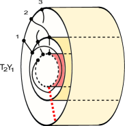
Figure 2: Toroidal representation of the product $T_{2}Y_{1}.$

4.3 Graphical Representation of the action of $Q_{i}$

4.3.1 The case $Q_{i}=\mathbb{1}$

We must confirm that our cubic/toroidal representation works for all the $\mathcal{D}_{N}\{Q\}$ axioms. We start by verifying (4.5), i.e. $Y_{1}Z_{2}Y^{-1}_{1}Z^{-1}_{2}=T^{2}_{1}$. From Figure 3, we see that this is satisfied by our cube representation.

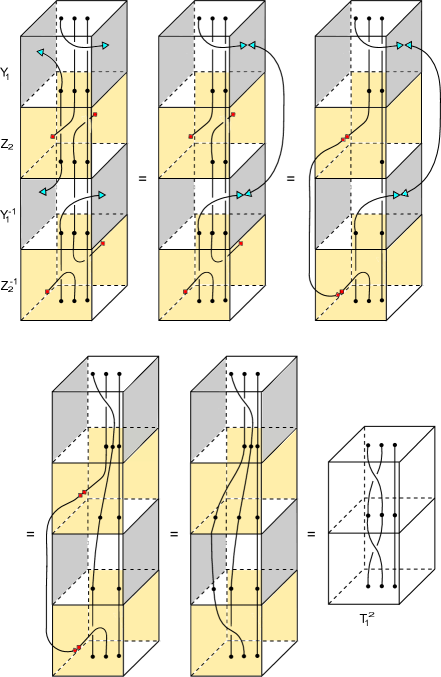
Figure 3: Step-by-step verification of the relation $Y_{1}Z_{2}Y_{1}^{-1}Z_{2}^{-1}=T_{1}^{2}$ in the cube representation.

(4.6) and (4.7) must also hold in our representation, of course. These are the relations that depend explicitly on the elements $Q_{i}$. In fact, they give us various ways of writing the $Q_{i}$; for example, in the $N=3$ case, we find $Q_{3}=\sigma Z_{1}\sigma^{-1}Z^{-1}_{3}$. We have pictorial representations for all the generators on the right-hand side of this relation, so we may explicitly find the pictorial representation of $Q_{3}$. From Figure 4, we see that $Q_{3}$ acts only on the third strand while leaving the other two untouched. For clarity, we have indicated the twisting using arrows; one must start form the top of the third strand and follow the arrows around all faces of the cube.

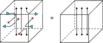
Figure 4: Pictorial representation of $Q_{3}=\sigma Z_{1}\sigma^{-1}Z^{-1}_{3}$. Pulling all strands tight yields the identity.

This is the pictorial representation of $Q_{3}$. By pulling the strands tight, we find that this is precisely the operator which leaves the strands entirely alone: the identity $\mathbb{1}$, namely, the trivial braid. This result is not unique to $Q_{3}$; we find that the graphical representation for each of the $Q$s is simply the identity.

Although this cube representation is successful in describing the $T_{i}$, $Y_{i}$ and $Z_{i}$ generators of $\mathcal{D}_{N}\{Q\}$, it still only allows the $Q_{i}$ to be represented by trivial braids, and so is really only valid when $Q_{i}=\mathbb{1}$. Therefore, this is simply a representation of $\mathcal{D}_{N}\{Q\}/\langle Q_{i}\rangle$, i.e. the elliptic braid group [9, 10] (see Figure 1). However, if we wish to allow for values of $Q_{i}$ other than unity, we need to modify our cube representation in some way, which we now describe.

4.3.2 The General Case $Q_{i}\neq\mathbb{1}$: Introducing Ribbons

To obtain a nontrivial pictorial representation which accommodates $Q_{i}\neq\mathbb{1}$, we modify our cube representation by replacing the strands by ribbons. This modification is not unmotivated: in order to extend the $\mathcal{A}_{N}\{Q\}$ representation to one for a $\mathcal{D}_{N}\{Q\}$, we increased the dimension of our space from two to three, and so it is reasonable to increase the dimension of our strands.

Doing so is precisely what we need in order for our representation to work for all $\mathcal{D}_{N}\{Q\}$s, not just those where the $Q_{i}=\mathbb{1}$. We therefore no longer braid one-dimensional strands, but do so instead with two-dimensional ribbons. This extra degree of freedom will enable us to completely describe a double affine $Q$-dependent braid group for any $Q_{i}$.

However, before we revisit the elements $Q_{i}$, we must verify that all of the previous $\mathcal{D}_{N}\{Q\}$ axioms still hold when using ribbons within our cube representation. It is straightforward to show that they do; to illustrate this point, we explicitly show (4.5), as this relation contains all three types of generators, the $T_{i}$, $Y_{i}$ and $Z_{i}$. (For clarity, we have coloured the front and back of each ribbon respectively by black and green.) This example, illustrated in Figure 5, also allows us to clearly lay out the braiding conventions that we use.

When the ribbon wraps in a left/right direction – representing a $Y_{i}$ operator – we use turquoise for the tips that are identified with each other. It is vital to stress that these link the left and right faces of the cube in a very particular fashion: the ribbon must pass through a left or right face of the cube oriented vertically. This condition ensures that the ribbon doesn’t twist while wrapping around the cube.

In a similar fashion, the ribbons representing the $Z_{i}$ generators are coloured so that when a red tip is visible, this implies that the ribbon passes through either the back or front face of the cube. We require that whenever such a ribbon intersects the front or back face of the cube, it does so oriented horizontally.

These conventions give Figure 5 for $Y_{1}Z_{2}Y^{-1}_{1}Z^{-1}_{2}=T^{2}_{1}$, and pulling the ribbons tight we can clearly see that the relation holds. All of the other relations are satisfied in a similar manner.

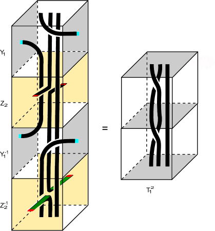
Figure 5: The relation $Y_{1}Z_{2}Y_{1}^{-1}Z_{2}^{-1}=T_{1}^{2}$ using ribbons instead of strands. Note the colour conventions.

One of the major advantages of our cube-ribbon representation is that specific crossing rules are not required when one ribbon crosses another. This is due to the fact that, following the conventions outlined above, the ribbons can braid in three distinct orthogonal directions and hence no such rules are necessary. In contrast, for framed braids in an infinitely long strip as in [14] more complicated crossing conditions are needed.

We now revisit the relation $Q_{3}=\sigma Z_{1}\sigma^{-1}Z^{-1}_{3}$ which, when represented by 1-dimensional strands, was equivalent to the identity element. Now using ribbons instead of strands, we construct the pictorial representation of $Q_{3}$. (For clarity, we show only the third ribbon, as this is the only one which behaves nontrivially.) Keeping with the colour convention defined earlier, we obtain $Q_{3}$, and, by pulling the ribbons tight, yields the key result we require: a twist in the ribbon is created! This important result is illustrated in Figure 6 below.

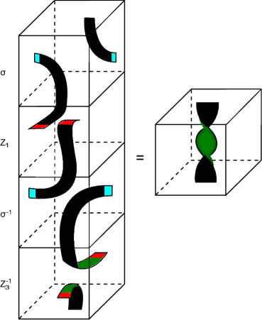
Figure 6: $Q_{3}$, the creation of a twist in the third ribbon. The full anticlockwise twist makes clearly visible both front and back faces of the ribbon, coloured black and green respectively. Note that we illustrate only the third ribbon.

As this is the most important feature of our ribbon representation, let us explain in detail how this comes about: in constructing $\sigma Z_{1}\sigma^{-1}Z^{-1}_{3}$, both the black and green faces of the ribbon are clearly visible. Upon closer inspection, we see that the ribbon undergoes a full anticlockwise twist in going from the top face to the bottom one. First, the front black face of the ribbon is visible. Then, having undergone half an anticlockwise twist, the back green face becomes visible until finally the full anticlockwise twist leaves the black face facing forwards.

This significant result can be generalised. We have just shown that in our cube-ribbon representation $Q_{3}$ creates a twist in the third ribbon. It is easily shown, following the construction of $Q_{3}$, that in our particular representation the action of $Q_{i}$ is to create a single full anticlockwise twist in the $i^{th}$ ribbon.

As the creation of a full anticlockwise twist in the ribbon may be somewhat difficult to visualise we have included a more rigorous argument to convince the reader in Appendix B.

Other expressions could be used to determine $Q_{i}$; for example, (4.6) gives

$$Q_{i} = Y_{i}\left(\prod_{j=1}^{N}Z_{j}\right)Y^{-1}_{i}\left(\prod_{j=1}^{N}Z^{-1}_{j}\right).$$

Or we could use (4.8): $Q_{i}=\sigma^{N}Z_{i}\sigma^{-N}Z^{-1}_{i}$. For these and any other representation for $Q_{i}$, the result is the same, namely, $Q_{i}$ creates a single full anticlockwise twist in the $i^{th}$ ribbon.

We can also verify that an expression like $Z_{3}\sigma Z_{1}^{-1}\sigma^{-1}$, which the $\mathcal{D}_{N}\{Q\}$ axioms require to be $Q^{-1}_{3}$ for $N=3$, is indeed a full clockwise twist in the third ribbon, again totally consistent with our interpretation of $Q_{i}$.

The interpretation of $Q_{i}$ is now clear: it is the generator that creates a full anticlockwise twist in the $i^{th}$ ribbon. Similarly $Q^{-1}_{i}$ creates a full clockwise twist in the $i^{th}$ ribbon. As these are no longer trivial actions on the ribbons, we have a pictorial representation for $Q_{i}\neq\mathbb{1}$, and a full description for $\mathcal{D}_{N}\{Q\}$.

5 Double Affine Hecke Algebras

In the previous section we highlighted the fact that the elliptic braid group is given by $\mathcal{D}_{N}\{Q\}$/$\langle Q_{i}\rangle$. Similarly readers familiar with double affine Hecke algebras [1, 11] may recognise that our definition of a $\mathcal{D}_{N}\{Q\}$ closely resembles that of a double affine Hecke algebra (DAHA) without the Hecke relation. We will in fact show precisely how to obtain a DAHA given our construction of a double affine $Q$-dependent braid group $\mathcal{D}_{N}\{Q\}$.

5.1 The Double Affine Hecke Algebra within $\mathcal{D}_{N}\{Q\}$

Consider the subgroup $\mathcal{C}$ of the $Q$-dependent braid group $\mathcal{B}_{N}\{Q\}$ defined as

$$\mathcal{C} = \langle Q_{i}Q^{-1}_{i+1},i=1,\ldots,N-1\rangle.$$

It can easily be shown that $\mathcal{C}$ is a normal subgroup of $\mathcal{B}_{N}\{Q\}$, and so we can construct the quotient $\mathcal{G}=\mathcal{B}_{N}\{Q\}/\langle\mathcal{C}\rangle$, which is precisely the group we require to define a DAHA. Within $\mathcal{G}$, the $Q_{i}$ are indistinguishable from one another; therefore, we refer to each of their cosets $[Q_{i}]$ as $Q$. Most importantly, using (2.3)-(2.6), we see that $Q$ now commutes with not only the squares of the braid group generators $T^{2}_{i}$, but also with the $T_{i}$ themselves. We are now in a position to extend the quotient group $\mathcal{G}$ to a Hecke algebra.

5.2 The Hecke Algebra $\mathcal{H}_{N}(t)$

Before defining a DAHA, we must extend our quotient group $\mathcal{G}$ to an algebra in which the $T_{i}$ generators satisfy a particular relation; this defines the Hecke algebra.

Associate with $\mathcal{G}$ the Hecke algebra $\mathcal{H}_{N}(t)$. This is the group algebra of $\mathcal{G}$ over a field $k$ parametrised by $t\in k$ such that each generator $T_{i}$ satisfies the Hecke relation

$$\left(T_{i}-t^{1/2}\mathbb{1}\right)\left(T_{i}+t^{-1/2}\mathbb{1}\right) = 0.$$ (5.1)

It is worth noting that even though $T^{-1}_{i}$ was assumed to exist in $\mathcal{G}$, this relation gives its form explicitly:

$$T^{-1}_{i} = T_{i}-\left(t^{1/2}-t^{-1/2}\right)\mathbb{1}.$$

5.3 The Double Affine Hecke Algebra $\mathcal{D}_{N}(t,q)$

To complete the DAHA construction we must firstly extend the Hecke algebra $\mathcal{H}_{N}(t)$ to an Affine Hecke Algebra $\mathcal{A}_{N}(t)$. This is achieved with the introduction of $N$ invertible operators $Y_{i}$ which satisfy (3.1)-(3.3).

Recall that the $\mathcal{A}_{N}$ was fully generated by $Y_{1}$ and the $T_{i}$. It is perhaps worth pointing out that the affine Hecke algebra is also fully generated by $Y_{1}$ and the $T_{i}$, and we can reorder them as necessary. This was not true for the $\mathcal{A}_{N}\{Q\}$ as we need the full Hecke algebraic structure in order to consistently order the operators. For example, $T_{1}$ and $Y_{3}$ can be reordered as we like, but this is true for $T_{1}$ and $Y_{2}$ only if we invoke the Hecke relation:

$$T_{1}Y_{2} = Y_{2}T_{1}^{-1}$$

$$= Y_{2}\left[T_{1}-\left(t^{1/2}-t^{-1/2}\right)\mathbb{1}\right]$$

$$= Y_{2}T_{1}-\left(t^{1/2}-t^{-1/2}\right)Y_{2}.$$

Following [1, 4] we take a DAHA $\mathcal{D}_{N}(t,q)$ of type $A$ to be the algebra generated by $T_{i}$, $Y_{i}$ and $Z_{i}$ which satisfy equations (2.1)-(2.2), the Hecke relation (5.1) along with (3.1)-(3.3) and (4.1)-(4.3).

In addition to these the $Y_{i}$ and $Z_{i}$ obey the intertwining relations [1]

$$Y_{1}Z_{2}Y^{-1}_{1}Z^{-1}_{2} = T^{2}_{1},$$ (5.2)

$$Y_{i}\left(\displaystyle\prod_{j=1}^{N}Z_{j}\right) = q\left(\displaystyle\prod_{j=1}^{N}Z_{j}\right)Y_{i},$$ (5.3)

$$Z_{i}\left(\displaystyle\prod_{j=1}^{N}Y_{j}\right) = q^{-1}\left(\displaystyle\prod_{j=1}^{N}Y_{j}\right)Z_{i},$$ (5.4)

where $q\in k$.

(As in the $\mathcal{D}_{N}\{Q\}$ (5.4) is not independent of the other relations, although it is often included in the literature as part of the definition of a DAHA.)

One must note that unlike our definition of the $\mathcal{D}_{N}\{Q\}$ where we have a set of elements $Q_{i}$, in the DAHA $q$ is simply a parameter. So a DAHA $\mathcal{D}_{N}(t,q)$ depends on the two variables $t,q$. This is entirely consistent with our construction of a DAHA from $\mathcal{D}_{N}\{Q\}$ via the quotient group $\mathcal{G}$ if we set $Q=q\mathbb{1}$. We therefore have a representation of a DAHA in $\mathcal{B}_{N}\{Q\}/\langle\mathcal{C}\rangle$ when we impose $Q=q\mathbb{1}$.

In terms of the cube representation we can replace a ribbon with a full anticlockwise twist by one with no twist at all, only if we multiply the resulting cube by a factor of $q$. One may see this explicitly in Figure 6. As a result, one may view this twist as the first Reidemeister move on a ribbon:

Therefore the interpretation of $q$ is clear: it is the multiplicative factor in front of a DAHA element whenever we replace a ribbon with a full anticlockwise twist by one with no twist at all. Furthermore since $q$ does not describe the actual position of the twist in the ribbon, one can have a factor of $q^{n}$ in front of a DAHA element corresponding to $n$ anticlockwise twists occurring anywhere in the cube. As there is no restriction on what value $q$ can take, we are not limited to the case $q$=1 and have a pictorial representation that fully describes any DAHA.

6 Summary and Discussion

In this paper we have defined and presented a graphical representation of the double affine $Q$-dependent braid group. Following the method of extending the pictorial representation of the $Q$-dependent braid group to one for an $\mathcal{A}_{N}\{Q\}$, we found that all of the relations not explicitly involving the operators $Q_{i}$ could be satisfied by a $\mathcal{D}_{N}\{Q\}$ depicted using $1$-dimensional strands embedded in a cube whose opposing vertical sides were identified, i.e. a hollowed-out toroid.

This representation was consistent only for a $\mathcal{D}_{N}\{Q\}$ where all the $Q_{i}=\mathbb{1}$; that is, the elliptic braid group. However, by replacing the strands with ribbons, our cube representation allowed us to capture all aspects of a $\mathcal{D}_{N}\{Q\}$ and gave us a nice interpretation of the action of any $Q_{i}$ as a single full anticlockwise twist in the $i^{th}$ ribbons. We thus obtain an intuitive pictorial representation which clearly incorporates all of the structure of the more abstract $\mathcal{D}_{N}\{Q\}$.

We showed that our new graphical representation is also valid for all DAHAs. Our definition of a $\mathcal{D}_{N}\{Q\}$ reduced to one of a double affine Hecke algebra simply by attaching the Hecke algebra to one of its quotient groups. The DAHA depends on two parameters $t$ and $q$. We found that graphically, the parameter $q$ corresponds to a full anticlockwise twist in the ribbon.

By construction, our representation should be closely related to tangles and knot theory. Using elementary tangles via Reidemeister moves to describe this algebra appears quite possible; in fact, the replacement of a full twist by a factor of $q$ is very much a Reidemeister-like move. This would indicate a relation between our cube-ribbon representation and elementary tangle representations of affine Hecke algebras; we hope to look further into this suspected relationship.

Similarly, transforming this cube-ribbon representation to an equivalent matrix representation is an interesting challenge. We hope to use our new pictorial representation to bring this closer to reality.

Appendix A

In this Appendix, we show that $\prod_{j=1}^{N}Y_{j}=\sigma^{N}$. Although this identity is already well-known [1], we present a proof for the interested reader.

Define the operator $P_{k}$ by

$$P_{k}: = \sigma^{k}\left(T_{1}\ldots T_{k}\right)^{-1}\left(T_{2}\ldots T_{k+1}\right)^{-1}\ldots\left(T_{N-k}\ldots T_{N-1}\right)^{-1}.$$ (A.1)

We want to show by induction that this is equal to $P_{k}=\displaystyle\prod_{j=N-k+1}^{N}Y_{j}$.

1. For $k=1$:

   $$P_{1} := \sigma^{1}\left(T_{1}\right)^{-1}\left(T_{2}\right)^{-1}\ldots\left(T_{N-1}\right)^{-1}$$

   $$= \sigma T^{-1}_{1}T^{-1}_{2}\ldots T^{-1}_{N-1}$$

   $$= Y_{N},$$

   so $P_{1}$ is indeed equal to $\displaystyle\prod_{j=N-1+1}^{N}Y_{j}=Y_{N}$, and the assertion is true for $k=1$.

2. Now assume that our assertion is true for some $k$, namely,

   $$P_{k} = \sigma^{k}\left(T_{1}\ldots T_{k}\right)^{-1}\left(T_{2}\ldots T_{k+1}\right)^{-1}\ldots\left(T_{N-k}\ldots T_{N-1}\right)^{-1}=\prod_{j=N-k+1}^{N}Y_{j}.$$

   If this holds, then $P_{k}Y_{N-k}$ is $\displaystyle\prod_{j=N-k}^{N}Y_{j}$ because all the $Y_{i}$ commute. Using $Y_{N-k}=T_{N-k}\ldots T_{N-1}\sigma T^{-1}_{1}\ldots T^{-1}_{N-k-1}$, we can rewrite this same expression as

   $$P_{k}Y_{N-k} = \left[\sigma^{k}\left(T_{1}\ldots T_{k}\right)^{-1}\left(T_{2}\ldots T_{k+1}\right)^{-1}\ldots\left(T_{N-k}\ldots T_{N-1}\right)^{-1}\right]$$

   $$\times\left[T_{N-k}\ldots T_{N-1}\sigma T^{-1}_{1}\ldots T^{-1}_{N-k-1}\right]$$

   $$= \left[\sigma^{k}\left(T_{1}\ldots T_{k}\right)^{-1}\left(T_{2}\ldots T_{k+1}\right)^{-1}\ldots\left(T_{N-k-1}\ldots T_{N-2}\right)^{-1}\right]$$

   $$\times\left[\sigma T^{-1}_{1}\ldots T^{-1}_{N-k-1}\right].$$

   Using $T^{-1}_{i}\sigma=\sigma T^{-1}_{i+1}$, all $\sigma$s can be moved to the left:

   $$P_{k}Y_{N-k} = \left[\sigma^{k+1}\left(T_{2}\ldots T_{k+1}\right)^{-1}\left(T_{3}\ldots T_{k+2}\right)^{-1}\right]\ldots$$

   $$\dots\left[\left(T_{N-k}\ldots T_{N-1}\right)^{-1}T^{-1}_{1}\ldots T^{-1}_{N-k-1}\right].$$

   $T_{i}$ commutes with all other $T$s except $T_{i+1}$ and $T_{i-1}$, so we may pull the rightmost operators $T_{1}^{-1}$ to $T_{N-k-1}^{-1}$ as far as possible to the left:

   $$P_{k}Y_{N-k} = \sigma^{k+1}\left[\left(T_{2}\ldots T_{k+1}\right)^{-1}T_{1}^{-1}\right]\left[\left(T_{3}\ldots T_{k+2}\right)^{-1}T_{2}^{-1}\right]\ldots$$

   $$\dots\left[\left(T_{N-k}\ldots T_{N-1}\right)^{-1}T^{-1}_{N-k-1}\right]$$

   $$= \sigma^{k+1}\left(T_{1}\ldots T_{k+1}\right)^{-1}\left(T_{2}\ldots T_{k+2}\right)^{-1}\ldots\left(T_{N-k-1}\ldots T_{N-1}\right)^{-1}.$$

   But (A.1) tells us that this is precisely the definition of $P_{k+1}$. Thus, $P_{k}Y_{N-k}=P_{k+1}$, so $P_{k+1}=\displaystyle\prod_{j=N-k}^{N}Y_{j}$ and our assertion holds for $k+1$ if it holds for $k$.

This therefore verifies that

$$\sigma^{k}\left(T_{1}\ldots T_{k}\right)^{-1}\left(T_{2}\ldots T_{k+1}\right)^{-1}\ldots\left(T_{N-k}\ldots T_{N-1}\right)^{-1} = \prod_{j=N-k+1}^{N}Y_{j}$$

for all $k=1,2,\ldots,N-1$. For $k=N-1$, this gives

$$\sigma^{N-1}\left(T_{1}\ldots T_{N-1}\right)^{-1} = \prod_{j=2}^{N}Y_{j}.$$

But $\sigma^{-1}(T_{1}\ldots T_{N-1})^{-1}=Y_{1}^{-1}$, so we find that

$$\prod_{j=1}^{N}Y_{j}=\sigma^{N}. \blacksquare$$

Appendix B

Here we show that the twist in the ribbon generated by $Q_{3}$ is precisely $2\pi$. We demonstrate this specifically for the case of $Q_{3}=\sigma Z_{1}\sigma^{-1}Z^{-1}_{3}$ as in Figure (6) where, from top to bottom, a full anticlockwise twist in the third ribbon is obtained. For clarity we illustrate only the third ribbon as it is the only one that behaves non-trivially.

Firstly let $z(s),(0\leq s\leq 1)$ denote the position of a point on the ribbon. Then $\hat{v}$ is the unit vector indicating the ribbon orientation and always lies on the surface of the ribbon. The direction of motion is given by the unit vector $\hat{u}$, where at all times $\hat{u}.\hat{v}=0$. The vector $\hat{w}=\hat{u}\times\hat{v}$ defines the normal to the ribbon.
So there is an orthogonal frame $g(s)=[\hat{u},\hat{v},\hat{w}]$ attached to each point on the ribbon as indicated in the diagram below.

We now follow a point as it travels down the ribbon. Attached to this point is the orthogonal frame $g(s)$. We impose that the ribbon cannot twist around the direction of motion, that is; $\omega.\hat{u}=0$ where $\omega$ is the angular velocity of the frame $g(s)$. We measure the degree of rotation of $g(s)$, between the top and bottom of the ribbon, relative to a fixed frame. This yields the size of the twist in the ribbon.

The Figure 7 (a) below shows the frame $g(s)$ at various points along the ribbon, from the top of the ribbon labelled point (A), to the bottom of the ribbon; point (B). Between these points we show that the moving frame $g(s)$ undergoes a full $2\pi$ rotation relative to the inertial reference frame ($\hat{x},\hat{y},\hat{z}$).

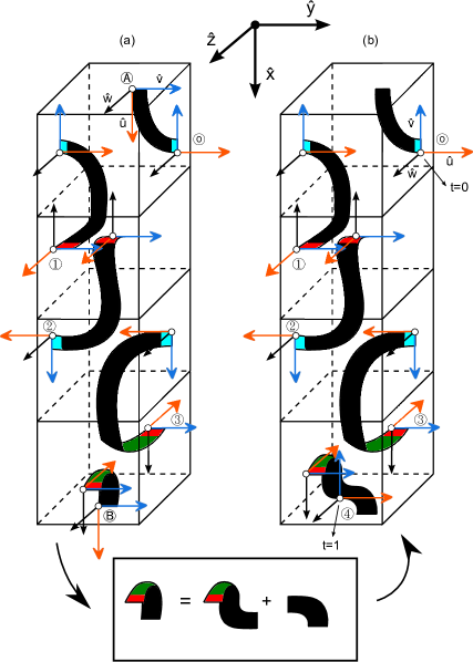
Figure 7: Figure (a) shows $g(s)$ at various points along the ribbon $Q_{3}=\sigma Z_{1}\sigma^{-1}Z^{-1}_{3}$. In Figure (b) we redraw the relation such that between times $t=0$ and $t=1$ one can see $\hat{u}$ rotating by $2\pi$ in the $\hat{y}-\hat{z}$ plane.

Notice that between points (A) and (0), the ribbon itself does not undergo any rotation. Therefore without losing any information we can measure the twist starting from point (0), which we now call time $t=0$, as in Figure 7 (b).
Furthermore in Figure 7 (b), the bottom of the ribbon is redrawn in such a way that the extra turns do not contribute to the overall twist. Then following $g(s)$ from $t=0$ to $t=1$, one can immediately see that $\hat{u}$ rotates only in the $\hat{y}-\hat{z}$ plane. In fact it does exactly a $2\pi$ clockwise rotation. So at any time $t$, $\hat{u}$ can be written as follows:

$\hat{u}(t)=\cos(2\pi t)\hat{y}+\sin(2\pi t)\hat{z}$.

One can easily check this holds. For example at time $t=1/2$, $\hat{u}(1/2)=-\hat{y}$. This is verified upon inspection of point (2) in the diagram.

Further inspection reveals that as $\hat{u}$ rotates in the $\hat{y}-\hat{z}$ plane, the vectors $\hat{v}$ and $\hat{w}$ rotate in a clockwise fashion around $\hat{u}$.
We introduce a frame $[\hat{e}_{1},\hat{e}_{2},\hat{e}_{3}]$, where $\hat{e}_{1}=\hat{u}$ and $\hat{e}_{2}$, $\hat{e}_{3}$ are functions of $\hat{v}$ and $\hat{w}$, to measure the rotation of $\hat{v}$ and $\hat{w}$ around $\hat{u}$. Impose that at $t=0$, $\hat{e}_{1}=\hat{u},\hat{e}_{2}=\hat{v}$ and $\hat{e}_{3}=\hat{w}$. It is important to note that $\hat{e}_{1}=\hat{u}$ at all times; that is we have $\hat{u}(t)=\hat{e}_{1}$.
Therefore in terms of this frame $[\hat{e}_{1},\hat{e}_{2},\hat{e}_{3}]$ we can write:

$\hat{v}(t)=\cos(2\pi t)\hat{e}_{2}-\sin(2\pi t)\hat{e}_{3}$,

$\hat{w}(t)=\sin(2\pi t)\hat{e}_{2}+\cos(2\pi t)\hat{e}_{3}$.

Again these can easily be verified through simple substitution and by referring to the above diagram.

$\hat{u}$ was fixed to $\hat{e}_{1}$ so in terms of the inertial reference frame we have:

$\hat{e}_{1}(t)=\cos(2\pi t)\hat{y}+\sin(2\pi t)\hat{z}$.

Following the vector $\hat{e}_{2}$ between $t=0$ and $t=1$ we see that it always points in the negative $\hat{x}$ direction. This implies that:

$\hat{e}_{2}(t)=-\hat{x}$.

Since $[\hat{e}_{1},\hat{e}_{2},\hat{e}_{3}]$ form an orthogonal frame we must have that:

$\hat{e}_{3}(t)=-\sin(2\pi t)\hat{y}+\cos(2\pi t)\hat{z}$.

Finally in terms of the fixed frame ($\hat{x},\hat{y},\hat{z}$);

$$\hat{u}(t) = \cos(2\pi t)\hat{y}+\sin(2\pi t)\hat{z},$$

$$\hat{v}(t) = -\cos(2\pi t)\hat{x}+{\sin}^{2}(2\pi t)\hat{y}-\sin(2\pi t)\cos(2\pi t)\hat{z},$$

$$\hat{w}(t) = -\sin(2\pi t)\hat{x}-\sin(2\pi t)\cos(2\pi t)\hat{y}+{\cos}^{2}(2\pi t)\hat{z}.$$

One can clearly see that $\hat{v}$ undergoes a full $2\pi$ clockwise rotation from $t=0$ to $t=1$. $\hat{v}$ lies on the ribbon surface at all times, therefore requiring the ribbon to undergo the same rotation. This yields precisely the required result; $Q_{3}$ creates a full anticlockwise twist in the third ribbon.

References

- [1] I. Cherednik, Double Affine Hecke Algebras, Cambridge University Press (2005)
- [2] I. Cherednik, “Nonsymmetric Macdonald Polynomials”, Int. Math. Res. Not. 10 (1995) 483
- [3] T. Jolicoeur and J. G. Luque, “Highest Weight Macdonald and Jack Polynomials”, J. Phys. A: Math. Theor. 44 (2011) 055204
- [4] M. Kasatani, “Subrepresentations in the Polynomial Representation of the Double Affine Hecke Algebra of Type at ”, Int. Math. Res. Not. 28 (2005) 1717
- [5] B. Feigin, M. Jimbo, T. Miwa and E. Mukhin, “Symmetric Polynomials Vanishing on the Shifted Diagonals and Macdonald Polynomials”, Int. Math. Res. Not. 18 (2003) 1015
- [6] M. Kasatani and V. Pasquier, “On Polynomials Interpolating between the Stationary State of a Model and a Q.H.E. Ground State” Commun. Math. Phys. 276 (2007) 397
- [7] L. Kauffman, “State Models and the Jones Polynomial”, Topology 26 (1987) 395
- [8] V. F. R. Jones, “A Polynomial Invariant for Knots via von Neumann Algebras”, Bull. Amer. Math. Soc. 12 (1985) 103
- [9] J. Birman, “On Braid Groups”, Commun. Pure Appl. Math. 22 (1969) 41
- [10] G. P. Scott, “Braid Groups and the Group of Homeomorphisms of a Surface”, Proc. Camb. Phil. Soc. 68 (1970) 605
- [11] D. Bernard, M. Gaudin, D. Haldane and V. Pasquier, “Yang-Baxter Equation in Spin Chains with Long Range Interactions”, J. Phys. A 26 (1993) 5219
- [12] B. Ion, “Involutions of Double Affine Hecke Algebras”, Compositio Math. 139 No. 1 (2003) 67
- [13] E. Artin, “Theory of Braids”, Annals of Mathematics 48 (1947) 101
- [14] K. H. Ko and L. Smolinsky, “The Framed Braid Group and 3-Manifolds”, Proc. AMS 115 No. 2 (1992) 541
- [15] N. Wahl, Ribbon Braids and Related Operads, PhD Thesis, University of Oxford (2001)
- [16] V. G. Turaev, Quantum Invariants of Knots and 3-Manifolds, De Gruyter Studies in Mathematics, Vol. 18 (2010)