How well can cold-dark-matter substructures account for the observed lensing flux-ratio anomalies?

Abstract

Lensing flux-ratio anomalies are most likely caused by gravitational lensing by small-scale dark matter structures. These anomalies offer the prospect of testing a fundamental prediction of the cold dark matter (CDM) cosmological model: the existence of numerous substructures that are too small to host visible galaxies. In two previous studies we found that the number of subhalos in the six high-resolution simulations of CDM galactic halos of the Aquarius project is not sufficient to account for the observed frequency of flux ratio anomalies seen in selected quasars from the CLASS survey. These studies were limited by the small number of halos used, their narrow range of masses ($\sim(1-2)\times 10^{12}M_{\sun})$ and the small range of lens ellipticities considered. We address these shortcomings by investigating the lensing properties of a large sample of halos with a wide range of masses in two sets of high resolution simulations of cosmological volumes and comparing them to a currently best available sample of radio quasars. We find that, as expected, substructures do not change the flux-ratio probability distribution of image pairs and triples with large separations, but they have a significant effect on the distribution at small separations. For such systems, CDM substructures can account for a substantial fraction of the observed flux-ratio anomalies. For large close-pair separation systems, the discrepancies existing between the observed flux ratios and predictions from smooth halo models are attributed to simplifications inherent in these models which do not take account of fine details in the lens mass distributions.

1 Introduction

In the cold dark matter (CDM) model of structure formation a large population of dark matter subhalos is predicted to survive inside larger “host” halos. In galaxies like the Milky Way, their number vastly exceeds the number of observed satellites (about two dozen have been discovered in the Milky Way to date). This discrepancy can be readily understood on the basis of standard ideas on galaxy formation (Bullock et al., 2000; Benson et al., 2002; Cooper et al., 2010; Font et al., 2011; Guo et al., 2011). The model of Benson et al. (2002) predicted a population of ultrafaint satellites which was subsequently discovered in the SDSS (Tollerud et al., 2008; Koposov et al., 2008; Koposov et al., 2009). But even in this case, a large number of subhalos too small to make galaxies, should exist. These could, in principle, be detected from their strong gravitational lensing effects.

The present of subhalos could be revealed by the anomalous flux ratios seen in some multiply-lensed quasar systems. In these cases standard parametric lens models (e.g., a singular isothermal ellipsoid plus external shear, hereafter “SIE+$\gamma$”) can fit the image positions well, but not their flux ratios. This is known as the “anomalous flux ratio” problem (Kochanek 1991).

A number of possible solutions to the problem have been considered. For example, some of the flux-ratio anomalies could be accommodated by adding higher order multipoles to the ellipsoidal potential of the lensing galaxy. However, as the required amplitudes would be unreasonably larger than typically observed in galaxies and halo models, such a solution does not seem plausible (Evans & Witt 2003; Kochanek & Dalal 2004; Congdon & Keeton 2005; Yoo et al. 2006).

Propagation effects in the interstellar medium, such as galactic scintillation and scatter broadening, could also cause anomalous flux ratios. If so, one would expect a strong wavelength dependence of the anomalies measured at radio wavelengths, which has not been seen (Koopmans et al. 2003; Kochanek & Dalal 2004). Moreover, propagation effects cannot explain the fact that observed saddle (negative-parity) images often appear to be fainter than predicted by the standard lens models (e.g., Schechter & Wambsganss 2002; Kochanek & Dalal 2004).

The most promising explanation is that the anomaly is due to perturbations from small-scale structures hosted by lensing galaxies. Microlensing, which refers to lensing by stars, has been identified as a source of the flux-ratio anomalies observed at optical wavelengths for the multiple images of background quasars (Woźniak et al. 2000; Sluse et al. 2006; Keeton et al. 2006; Morgan et al. 2004, 2006, 2008; Vuissoz et al. 2008). In this case, the Einstein radius of a star in a foreground lensing galaxy is comparable to the size of the optical emission from the accretion disk of a background quasar; the magnification effect (on scales of the Einstein radius) alters the flux ratio between the images.

However, this is not the case for radio emission, which comes from a region much larger than the accretion disk. Any magnification due to foreground stars would be smeared out within the whole radio image zone and thus become insignificant. Therefore microlensing is not a likely explanation for the flux ratio anomalies measured at radio wavelengths (e.g., Kochanek & Dalal 2004).

Mao & Schneider (1998) first realized that dark matter substructures (on scales smaller than image separations $\sim 1\arcsec$ for typical lens and source redshifts) could explain the radio flux-ratio anomaly in B1422+231. Later studies showed that the presence of substructures in lensing galaxies can also explain the observed tendency for the brightness of saddle image to be suppresed (Schechter & Wambsganss 2002; Keeton 2003; Kochanek & Dalal 2004). Lensing subhalos has therefore emerged as one of the most convincing explanations for the radio flux-ratio anomalies. Such an explanation has important implications for cosmology since it provides a straightforward and very direct test of the CDM model.

There are about a dozen studies that use $N$-body simulations to test if the predicted CDM substructures are sufficiently abundant to explain the frequency of anomalous lenses in currently available samples. However, no consensus has emerged. While some of the studies suggest consistency between the CDM theory and observations (e.g., Dalal & Kochanek 2002; Bradač et al. 2004; Dobler & Keeton 2006; Metcalf & Amara 2012), others, including those by us (Xu et al. 2009; Xu et al. 2010), find otherwise (e.g., Mao et al. 2004; Amara et al. 2006; Macciò et al. 2006; Macciò & Miranda 2006; Chen et al. 2011).

Metcalf & Amara (2012) pointed out that the different conclusions between their study, which finds consistency between theory and data, and others, like ours, which do not (Xu et al. 2009; Xu et al. 2010) could be due to the following: (1) as the number density of substructures is small near the radii where multiple images form, relying on only a few projections of a small number of high-resolution halos, as we did, could produce biased results due to halo-to-halo variations; (2) as flux ratios are quite sensitive to the ellipticity of the main lens (Keeton et al. 2003), our restriction to a relatively small ellipticity (axis ratio = 0.8), instead of the full range of ellipticities in the main lens models, could also skew the results.

There are other factors that could weaken the conclusion in our studies. For example, the cosmological simulations that we have used contain only dark matter but no baryons, and this might change the subhalo survival rate and thus their spatial distributions. This effect is negligible for substructures in galaxies which have very large (or infinite) mass-to-light ratios but could be important in groups and clusters. Unfortunately, current simulations are not yet sufficiently large or accurate to investigate this problem. We will have to rely on using the next-generation hydrodynamical cosmological simulations to accommodate such effects.

Another limitation of our previous work is that we focused exclusively on the six Milky Way-sized dark matter halos from the Aquarius project (Springel et al. 2008). However, massive ellipticals galaxies, which comprise 80%-90% of observed lenses (Keeton et al., 1998; Kochanek et al., 2000; Rusin et al., 2003) are more likely to occur in group-sized halos which are ten times more massive. Since the subhalo abundance increases rapidly with increasing host halo mass (e.g. De Lucia et al., 2004; Gao et al., 2004; Zentner et al., 2005; Wang et al., 2012), the subhalo population in the Aquarius simulations may not fairly represent that in group-sized dark matter halos and this could have led us to underestimate the probability of flux-ratio anomalies.

In this paper we address most of the issues mentioned above. We use two sets of high-resolution cosmological CDM simulations - from the Aquarius (Springel et al., 2008) and Phoenix (Gao et al., 2012) - to attempt to answer the question of how well do cold-dark-matter substructures account for the observed lensing flux-ratio anomalies. The paper is organized as follows: In Sect.2, we review the generic relations in cusp (Sect.2.1) and fold (Sect.2.2) lenses. In Sect.2.3, we present our observational sample of eight lenses, all of which have radio measurements for both cusp and fold relations. In Sect.3, we present a method to represent numerically massive elliptical lenses and their subhalo populations. To model the potentials of a general host lens population, in Sect.3.1, we use a technique similar to that of Keeton et al. (2003). In Sect.3.2, we rescale both the Aquarius and Phoenix simulations to group-sized dark matter halos, add the rescaled subhalos to the smooth lens potentials, and estimate their perturbation effects on the flux ratios of quadruply-lensed quasar images. The resulting flux-ratio probability distributions are presented in Sect.4, where comparisons are made to observations and to previous studies. Due to the limitations of generalized smooth lens potentials and image configurations, we have further carried out a detailed investigation of each system in the currently available sample; results presented in Sect.5. A discussion and our conclusions are given in Sect.6.

The cosmology we adopt here is the same as that for both sets of simulations that we have used in this work, with a matter density $\Omega_{\rm m}$ = 0.25, cosmological constant $\Omega_{\Lambda}$ = 0.75, Hubble constant $h=H_{0}/(100{\rm\,km\,s^{-1}}\,{\rm Mpc}^{-1})=0.73$ and linear fluctuation amplitude $\sigma_{8}=0.9$. These values are consistent with cosmological constraints from the WMAP 1- and 5-year data analyses (Spergel et al. 2003; Komatsu et al. 2009), but differ from Planck 2013 results (Planck Collaboration et al. 2013), where $h=0.67$ and $\sigma_{8}=0.829\pm 0.012$. However, we do not expect these differences in cosmological parameters to have any significant consequences for our conclusions.

2 Generic relations in cusp lenses and fold lenses

There are three generic configurations of four-image lenses (see Fig.1): (1) a source located near a cusp of the tangential caustic will produce a “cusp” configuration, where three images form close to each other around the critical curve on one side of the lens; (2) a source located near the caustic and between two adjacent cusps will produce a “fold” configuration, where a pair of images form close to each other near the critical curve; (3) a source located far away from the caustic, i.e., in the central region of the caustic, will produce a “cross” configuration, where all four images form far away from each other and away from the critical curve. Close triple images in cusp lenses and close pair images in fold lenses are the brightest images among the four, as they form close to the (tangential) critical curve.

There are some universal magnification relations for the triple and pair images in cusp and fold systems under smooth lens potentials. These generic relations assist one to identify small-scale perturbations via identifying violations to these generic magnification relations, without requiring detailed lens modeling for individual systems.

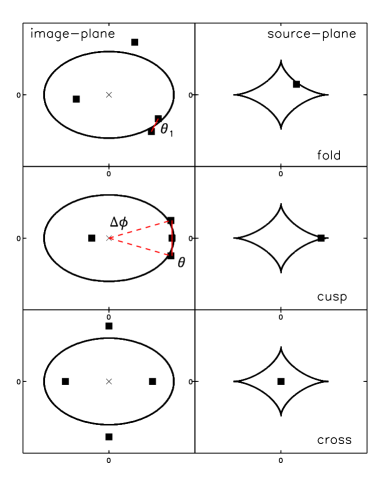
Figure 1: Three basic image configurations: fold (top), cusp (middle), and cross (bottom), with respect to the tangential critical curves in the image plane (on the left), and corresponding source positions with respect to the central caustics in the source plane (on the right). The image separation $\theta_{1}$ of a close pair is labeled for the fold configuration; image opening angle $\Delta\phi$ and separation $\theta$ of a close triplet are labeled for the cusp configuration.

2.1 The cusp relation and the violation due to small-scale structures

In any smooth lens potential that produces multiple images (of a single source) of a cusp configuration, a specific magnification ratio (i.e., also the flux ratio) of the image triplet will approach zero asymptotically, as the source approaches a cusp of the tangential caustic. This is known as the “cusp relation” (Blandford & Narayan 1986; Schneider & Weiss 1992; Zakharov 1995; Keeton et al. 2003), mathematically defined as:

$$R_{\rm cusp}\equiv\frac{|\mu_{A}+\mu_{B}+\mu_{C}|}{|\mu_{A}|+|\mu_{B}|+|\mu_{C}|}\rightarrow 0~{}~{}~{}(\Delta\beta\rightarrow 0),$$ (1)

where $\Delta\beta$ is the offset between the source and the nearest cusp of the caustic, $\mu_{A,B,C}$ denote the triplet’s magnifications, whose signs indicate image parities.

Because $\Delta\beta$ cannot be directly measured, we therefore follow the practice of Keeton et al. (2003), using $\Delta\phi$ and $\theta/\theta_{\rm Ein}$ to quantify a cusp image configuration. As labeled in Fig.1, $\Delta\phi$ is defined as the angle between the outer two images of a triplet, measured from the position of the lens centre; $\theta/\theta_{\rm Ein}$ is the maximum image separation among the triplet, normalized by the Einstein radius $\theta_{\rm Ein}$. In general, when the source moves towards the nearest cusp, both $\Delta\phi$ and $\theta/\theta_{\rm Ein}$ will decrease to zero.

Small-scale structures, either within the lens or projected by chance along the line of sight, will perturb the lens potential and alter fluxes of one or more images. In this case, $R_{\rm cusp}$ will become unexpectedly large. The cusp relation, i.e., $R_{\rm cusp}\rightarrow 0$ when $\Delta\beta\rightarrow 0$, will then be violated (e.g., see Fig.2 of Xu et al. 2012 for an illustration).

2.2 The fold relation and the violation due to small-scale structures

For an image pair in a fold configuration produced by any smooth lens potential, there is also a generic magnification relation, namely the “fold relation” (Blandford & Narayan 1986; Schneider & Weiss 1992; Schneider et al. 1992; Petters et al. 2001). In this paper, we take the form as in Keeton et al. (2005):

$$R_{\rm fold}\equiv\frac{|\mu_{\rm min}|-|\mu_{\rm sad}|}{|\mu_{\rm min}|+|\mu_{\rm sad}|}\rightarrow 0~{}~{}~{}(\Delta\beta\rightarrow 0),$$ (2)

where $\Delta\beta$ is the offset of the source from the fold caustic, $\mu_{\rm min,sad}$ denote magnifications of the minimum ($\mu>0$) and saddle ($\mu<0$) images. To quantify a fold image configuration, similar to the practice of Keeton et al. (2005), we use $\theta_{1}/\theta_{\rm Ein}$ to indicate how close the pair of images are. As labelled in Fig.1, $\theta_{1}/\theta_{\rm Ein}$ is defined as the separation, in unit of the Einstein radius $\theta_{\rm Ein}$, between the saddle image and the nearest minimum image. When small-scale structures are present, $R_{\rm fold}$ will also become unexpectedly large; the fold relation, i.e., $R_{\rm fold}\rightarrow 0$ when $\Delta\beta\rightarrow 0$, will then be violated.

We can study small-scale structures by investigating the resulting violations to the cusp and fold relations in extreme systems where $\Delta\beta\sim 0$. However, the detected number of such systems is zero. For observed lenses, $\Delta\beta\neq 0$, and the exact values of $R_{\rm cusp}$ and $R_{\rm fold}$ depend on $\Delta\beta$ and on the lens potentials. Without detailed lens modelling, we can identify cases of violations as outliers of some general distributions of $R_{\rm cusp}$ and $R_{\rm fold}$ for smooth lenses. A series of comprehensive and detailed studies on this topic have been carried out by e.g., Keeton et al. (2003, 2005), whose methods are largely followed in this work (see Sect.3.1).

2.3 A sample of cusp and fold lenses

As adding CDM substructures to smooth lens potentials would change the distributions of $R_{\rm cusp}$ and $R_{\rm fold}$, resulting in anomalous flux ratios, we can compare simulation results to a reasonable observational sample to see how well the CDM substructure models can explain observations. There are more than twenty lenses with $R_{\rm cusp}$ and $R_{\rm fold}$ measured at optical, near-infrared (NIR) and radio wavelengths (CfA-Arizona Space Telescope Lens Survey, http://cfa-www.harvard.edu/castles). Nearly half of them show anomalous flux ratios in the sense that the measured $R_{\rm cusp}$ and $R_{\rm fold}$ cannot be reproduced by the lens models that best fit their image positions (Keeton et al. 2003, 2005).

As the fluxes measured at optical and NIR (Sluse et al. 2013) wavelengths can be significantly affected by microlensing and dust extinction, we will only take those systems with $R_{\rm cusp}$ and $R_{\rm fold}$ measured at radio wavelengths.

In our previous studies, we used all (five) existing radio lenses that have triplet image opening angles $\Delta\phi\leqslant 120^{\circ}$. All of them have surprisingly large $R_{\rm cusp}$ values that cannot be reproduced by the best-fit lens models. In this work, we take all radio quads (four distinct point-like images from one single source) in either cusp or fold configurations that have both $R_{\rm cusp}$ and $R_{\rm fold}$ measurements. This forms a sample of a total of eight lenses; three “cusp”, and five “fold”.

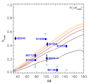
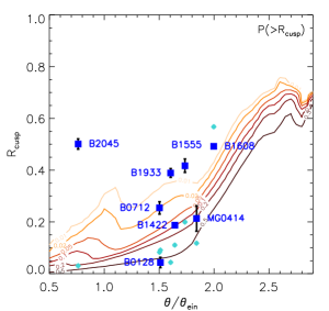
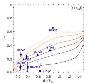
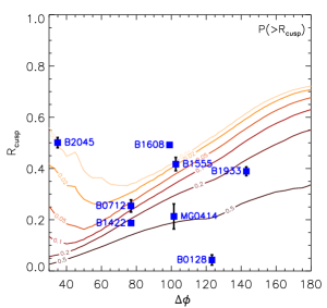
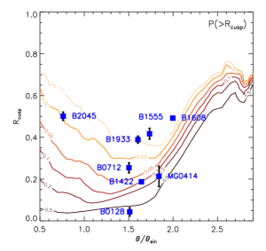
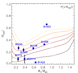
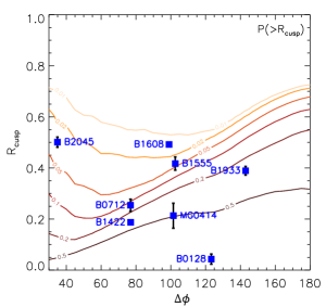
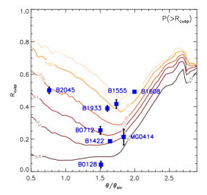
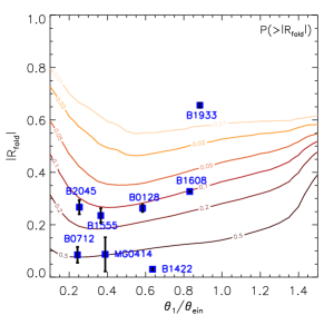
Figure 2: Probability contour maps of conditional probabilities $P(>R_{\rm cusp}\mid\Delta\phi)$ (left column), $P(>R_{\rm cusp}\mid\theta/\theta_{\rm Ein})$ (middle column) and $P(>|R_{\rm fold}|\mid\theta_{1}/\theta_{\rm Ein})$ (right column). Contour levels of 1, 2, 5, 10, 20 and 50 per cent (from light to dark) are plotted. Top: singular isothermal ellipsoidal potentials with axis ratio $q$ and higher-order perturbation amplitudes $a_{m}$ drawn from 847 observed galaxies (Hao et al. 2006), plus randomly oriented external shear. Middle: smooth potentials (as above) plus perturbations from a simulated subhalo population hosted by a Milky Way-sized halo of $M_{200}=10^{12}h^{-1}M_{\odot}$. Bottom: smooth potentials (as for the top panel) plus perturbations from a simulated subhalo population hosted by a group-sized halo of $M_{200}=5\times 10^{13}h^{-1}M_{\odot}$. More than $5\times 10^{6}$ realizations have been calculated for each case. Measured and model predicted flux ratios ($R_{\rm cusp}$ and $|R_{\rm fold}|$) of eight observed lenses are plotted as blue squares and cyan diamonds, respectively; measurement errors are also given. These distributions do not vary with the way that data are binned when using a reasonable range of bin sizes.

For each of the eight observed lenses, we take the basic image configuration measurements, namely, $\Delta\phi$, $\theta/\theta_{\rm Ein}$ and $\theta_{1}/\theta_{\rm Ein}$, as well as the measured and model predicted flux ratios of $R_{\rm cusp}$ (for the closest triple images) and $R_{\rm fold}$ (for the closest saddle-minimum image pairs), listed in Table 1. It can be seen that discrepancies at different levels exist between the observed flux ratios and the predictions from best-fit smooth models.

Table 1: Observed lenses with measurements of $R_{\rm cusp}$ and $R_{\rm fold}$ for the close triple images:

Lens	Type	$\Delta\phi$(∘)	$\theta/\theta_{\rm Ein}$	$R_{\rm cusp}$	$\theta_{1}/\theta_{\rm Ein}$	$R_{\rm fold}$	References
B0128+437	fold	123.3	1.511	0.043$\pm$0.020 (0.090)	0.584	0.263$\pm$0.014 (0.161)	1, 2
MG0414+0534	fold	101.5	1.841	0.213$\pm$0.049 (0.118)	0.388	0.087$\pm$0.065 ($-$0.029)	3, 4, 5, 6
B0712+472	cusp	76.9	1.503	0.254$\pm$0.024 (0.083)	0.243	0.085$\pm$0.030 ($-$0.037)	1, 7, 8, 9
B1422+231	cusp	77.0	1.643	0.187$\pm$0.004 (0.110)	0.636	$-$0.030$\pm$0.004 ($-$0.131)	1, 10, 11, 3
B1555+375	fold	102.6	1.735	0.417$\pm$0.026 (0.199)	0.365	0.235$\pm$0.028 (0.023)	1, 12
B1608+656	fold	99.0	1.997	0.492$\pm$0.002 (0.568)	0.831	0.327$\pm$0.003 (0.411)	13, 14
B1933+503	fold	143.0	1.605	0.389$\pm$0.017 (0.040)	0.884	0.656$\pm$0.009 (0.257)	15, 16, 17
B2045+265	cusp	34.9	0.762	0.501$\pm$0.020 (0.030)	0.253	0.267$\pm$0.027 ($-$0.163)	1, 9, 18, 19

Notes: the quoted $R_{\rm cusp}$ and $R_{\rm fold}$ are measurements at radio wavelengths; their uncertainties are derived from the uncertainties in flux measurements. Values in brackets are predicted by the best-fit lens model, see our Sect.5.1. References: (1) Koopmans et al. 2003; (2) Phillips et al. 2000; (3) Falco et al. 1999; (4) Lawrence et al. 1995; (5) Katz et al. 1997; (6) Ros et al. 2000; (7) Jackson et al. 1998; (8) Jackson et al. 2000; (9) Cfa-Arizona Space Telescope Lens Survey (CASTLES, see http://cfa-www.harvard.edu/castles); (10) Impey et al. 1996; (11) Patnaik et al. 1999; (12) Marlow et al. 1999; (13) Koopmans & Fassnacht 1999; (14) Fassnacht et al. 1996; (15) Cohn et al. 2001; (16) Sykes et al. 1998; (17) Biggs et al. 2000; (18) Fassnacht et al. 1999; (19) McKean et al. 2007; .

In order to see how observations would compare to smooth model predictions and how frequently they are expected to violate smooth predictions, we produce expected flux-ratio probability distributions with a total of $5\times 10^{6}$ realizations for a generalized smooth lens population, which are modelled by isothermal ellipsoidal potentials with axis ratios and high-order multipole perturbations drawn from 847 observed galaxies (Hao et al. 2006) plus external shear (see Sect.3.1 for more details).

The results are presented in the top panels of Fig.2, where probability contours of $P(>R_{\rm cusp}\mid\Delta\phi)$, $P(>R_{\rm cusp}\mid\theta/\theta_{\rm Ein})$ and $P(>|R_{\rm fold}|\mid\theta_{1}/\theta_{\rm Ein})$ are plotted. A small (large) probability $P$ means that it is less (more) likely for a flux ratio, either $R_{\rm cusp}$ or $|R_{\rm fold}|$, to be larger than a given value, at a given image configuration, described by $\Delta\phi$, $\theta/\theta_{\rm Ein}$ or $\theta_{1}/\theta_{\rm Ein}$.

On top of the probability contours in Fig.2, measured $R_{\rm cusp}$ and $|R_{\rm fold}|$ of the eight lenses in our sample are plotted as blue squares, together with measurement errors. Flux ratios predicted by the lens model that best fits image positions are also given, plotted as cyan diamonds. As can be seen, the majority of model predicted flux ratios satisfy $P\gtrsim 20\%$, while most of the measured flux ratios have probabilities well below such a percentage, suggesting such a smooth lens population on its own is unlikely to account for most of the observed flux ratio anomalies.

3 Realization of a massive elliptical lens and its subhalo population

In order to see how CDM substructures could affect the flux-ratio probablity distributions and how well they can account for the observed flux-ratio anomalies in our sample, we add simulated CDM subhalo populations to generalized smooth lens potentials and predict the flux-ratio probablity distributions in the presence of substructures. In this section, we present the method of the numerical realization of massive elliptical lenses (Sect.3.1) and their substructure populations (Sect.3.2).

3.1 Smooth lens model

To model the main lens halo (which is responsible for producing multiple images), we adopt Keeton et al. (2003) smooth lens modelling, which allows us to predict generic distributions for the cusp and fold relations and to see how well the observational sample follows such distributions in the absence of CDM substructures.

Keeton et al. (2003, 2005) studied the generic flux-ratio relations in cusp and fold lenses and showed that they have a weak dependence on the radial profile (from point mass to isothermal) of the lens potential, but are sensitive to ellipticity $e$($\equiv 1-q$, where $q$ is the axis ratio), higher-order multipole amplitude $a_{m}$ and external shear $\gamma_{\rm ext}$. In this work, we use a generalized isothermal ellipsoidal profile with an Einstein radius of 1.0$\arcsec$ and also take into account the three aspects above. Detailed lens modelling is given in the Appendix.

For choosing $e$ and $a_{m}$, we use results from Hao et al. (2006), who measured ellipticities and higher-order multipoles ($m=3,~{}4$) of 847 Sloan galaxies. The mean and scatter of these shape parameters ($\bar{e}=0.23$, $\sigma_{e}=0.13$, $\bar{a}_{3}=0.005$, $\sigma_{a_{3}}=0.004$, $\bar{a}_{4}=0.010$, $\sigma_{a_{4}}=0.012$) are comparable to the values reported for the galaxy samples used in Keeton et al. (2003, 2005).

We note that by using the observed galaxy morphology distributions, we implicitly assume that the shape of dark matter distribution follows baryons in the inner parts of the halo where strong lensing occurs. This has been supported by lensing observations from e.g., Koopmans et al. (2006) and Sluse et al. (2012).

It is also worth noting that although we draw shape parameters ($e$ and $a_{m}$) for lens modelling from a galaxy sample at lower redshifts ($z<0.2$), as addressed in Keeton et al. (2003, 2005), such distributions are not expected to be significantly different from those of the observed lensing galaxies at intermediate redshifts; observations have shown no significant evolution in the mass assembly history of early-type galaxies since $z\approx 1$ (Thomas et al. 2005; Koopmans et al. 2006).

Standard lens modelling would also include external shear, which is required to account for the lensing effect from the lens environments (e.g., Keeton et al. 1997, Sluse et al. 2012). We follow the practice of Keeton et al. (2003), assuming a lognormal distribution of $\gamma_{\rm ext}$ with a median of 0.05 and $\sigma_{\gamma}=0.2$ dex.

To add simulated CDM subhalos to the generalized host lens potentials, we take 3600 different projections of subhalo distributions, and add each of them to one realization of the host lens potential. For any given host lens potential, to maintain the possible correlation between ellipticities and high-order multipoles, we draw the combination of measured ($e$, $a_{3}$, $a_{4}$) from the observed galaxy sample of Hao et al. (2006). We then add a randomly orientated external shear. For each constructed lens potential, we carry out standard lensing calculations, finding images for source positions that are uniformly distributed inside the tangential caustic with a number density of 20000 per arcsec² in the source plane. This naturally ensures that each realization will be weighted by their four-image cross section. We do not consider magnification bias in our statistical analysis, however we discuss the possible consequence in Sect.4 and Sect.5. In total we generate $\sim 5\times 10^{6}$ four-image lensing systems for the final inspection of cusp and fold violations.

3.2 CDM subhalos from the Aquarius and Phoenix simulations

To populate smooth lens potentials with CDM substructures, we take two sets of high-resolution cosmological $N$-body simulations: the Aquarius (Springel et al. 2008) and Phoenix (Gao et al. 2012) simulation suites. The former is composed of six Milky Way-sized halos ($M_{200}\sim 10^{12}h^{-1}M_{\odot}$) and the latter consists of nine galaxy cluster-sized halos ($M_{200}\sim 10^{15}h^{-1}M_{\odot}$; $M_{200}$ here is referred to as the virial mass, defined as the mass within $R_{200}$, the radius within which the mean mass density of the halo is 200 times the critical density of the Universe).

In order to estimate the lensing effects from a subhalo population hosted by group-sized dark matter halos and to study their dependencies on host halo properties, we rescale all these fifteen halos from both simulations to host halos of $M_{200}=10^{12}h^{-1}M_{\odot},~{}10^{13}h^{-1}M_{\odot},~{}{\rm and}~{}5\times 10^{13}h^{-1}M_{\odot}$. It is noteworthy to mention that we only use $M_{200}$ of individual halos to work out their rescaling relations, it is the subhalos (not the main halos) that we take, rescale and then add to the constructed host lens potentials (as described in Sect.3.1).

We define a rescaling factor $\mathfrak{R}$, which is the ratio between $M_{200}$ of the group-sized halo and that of a simulated halo. We rescale the masses of subhalos accordingly by a factor of $\mathfrak{R}$, and velocities, sizes and halo-centric distances of subhalos by a factor of $\mathfrak{R}^{\frac{1}{3}}$, so that characteristic densities remain the same.

We also require that the minimum mass of subhalos in rescaled group-sized halos should go down to $10^{6\sim 7}h^{-1}M_{\odot}$, so that we can analyze the lensing effects from small-scale structures in a wide mass range; perturbations on scales below $10^{6}h^{-1}M_{\odot}$ are not expected to alter radio flux ratios due to finite source size effect (see detailed discussion in Xu et al. 2012). For this reason we take both simulations at their second resolution levels (level-2), at which the minimum resolved subhalos have masses about seven orders of magnitude below the virial masses of their hosts. This means that a (rescaled) halo of $M_{200}=10^{12}h^{-1}M_{\odot}$, $10^{13}h^{-1}M_{\odot}$ and $5\times 10^{13}h^{-1}M_{\odot}$ would host a complete sample of subhalos down to a mass of $\sim 2\times 10^{5}h^{-1}M_{\odot}$, $\sim 2\times 10^{6}h^{-1}M_{\odot}$ and $\sim 10^{7}h^{-1}M_{\odot}$, respectively.

In Sect.4, we present results of cusp and fold violations caused by (rescaled) subhalo populations from halos at different mass scales, so that we can see the dependence on host halo masses. In the following, we present the rescaled subhalo properties, including mass function, characteristic velocities, sizes and spatial distributions.

3.2.1 Subhalo mass function

From Sect.4.1 and Fig.13 of Gao et al. (2012), no significant difference is seen between the shapes of subhalo mass functions of cluster-sized Phoenix halos and of Milky Way-sized Aquarius halos. The number of Phoenix subhalos is higher by 35% than the number of Aquarius subhalos at any fixed subhalo-to-halo mass ratio $m_{\rm sub}/M_{200}$. This is because clusters are dynamically younger than galaxies, therefore there are more subhalos surviving the tidal destruction.

3.2.2 Spatial distributions and projection effects

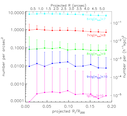
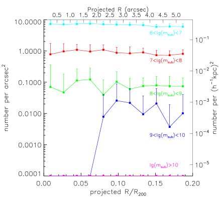
Figure 3: The radial distributions of projected subhalo number densities from the six level-2 Aquarius halos at redshift $z=0.6$. All halos are rescaled to $10^{12}h^{-1}M_{\odot}$. Five different subhalo mass ranges have been inspected: $10^{6\sim 7}h^{-1}M_{\odot}$ (cyan), $10^{7\sim 8}h^{-1}M_{\odot}$ (red), $10^{8\sim 9}h^{-1}M_{\odot}$ (green), $10^{9\sim 10}h^{-1}M_{\odot}$ (blue) and $>10^{10}h^{-1}M_{\odot}$ (pink). The $X$-axis at the top gives the projected radius in arcsec; the one at the bottom gives the projected radius normalized to $R_{200}$. The $Y$-axis on the left gives number per arcsec²; on the right gives number per ($h^{-1}$kpc)² (in physical scale). One-sided error bars indicate standard deviations. The top panel shows the result when 500 random projections are used per halo; the bottom panel when only three random projections are used per halo.

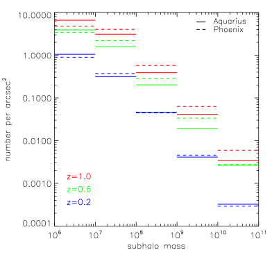
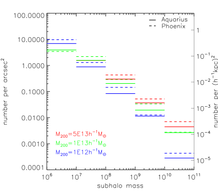
Figure 4: Projected subhalo number densities averaged within the central $R\leqslant 5\arcsec$ region, as a function of subhalo masses. The top panel shows the redshift dependence: host halos are rescaled to $M_{200}=10^{13}h^{-1}M_{\odot}$, taken at $z=0.2$ (blue), $z=0.6$ (green) and $z=1.0$ (red). The bottom panel shows the host mass dependence: halos taken at $z=0.6$, rescaled to $M_{200}=10^{12}h^{-1}M_{\odot}$ (blue), $10^{13}h^{-1}M_{\odot}$ (green) and $5\times 10^{13}h^{-1}M_{\odot}$ (red). 500 random projections are used per halo. The $Y$-axis on the left-hand side of each panel gives number per arcsec². The $Y$-axis on the right-hand side of the bottom panel also gives number per ($h^{-1}$kpc)² (in physical scale corresponding to a redshift at $z=0.6$). Solid lines show the number densities of the Aquarius subhalos; dashed lines are for the Phoenix subhalos.

From Sect.4.2 and Fig.15 of Gao et al. (2012), the spatial distribution of the Phoenix subhalos is slightly more concentrated (more abundant near the centre) than that of the Aquarius subhalos due to the assembly bias effect, as the Phoenix simulations start from high density regions.

For this work, the projected subhalo spatial distribution in terms of the radial distribution of projected subhalo number density is of particular interest, as it directly influences the lensing effects that subhalos induce. In this subsection, we show the mean projected spatial distributions obtained from averaging over hundreds of projections per host halo from both simulation suites.

The projected subhalo number density does not change significantly as a function of projected radius in the inner region of the host halo. This is seen for both Aquarius and Phoenix subhalos. Fig.3 plots mean projected spatial distributions of subhalos from six level-2 Aquaruis halos (rescaled to $M_{200}=10^{12}h^{-1}M_{\odot}$) at redshifts $z=0.6$, where 500 and 3 random projections are taken per halo for the left and right panels, respectively. The $Y$-axis on the left-hand side gives number per arcsec², on the right-hand side gives number per ($h^{-1}$kpc)² (in physical scale). Error bars show the standard deviations, and different colours indicate subhalos in different mass bins.

From Fig.3, we can also see how much our previous studies (Xu et al. 2009) could be biased from taking only three projections of each of the six Aquarius halos. Clearly, the projected spatial distribution of relatively massive subhalos ($m_{\rm sub}>10^{9}h^{-1}M_{\odot}$) could be strongly affected by small number statistics: the mean number densities drop to zero in the inner region if only three projections per halo are used, but will be restored if many more projections are taken per halo. Therefore, as Metcalf & Amara (2012) expected, our previous conclusion could have been affected due to halo-to-halo variations.

As the projected subhalo number densities remain constant in the inner part of a host halo, we take the mean values averaged within the central $R\leqslant 5\arcsec$ region and study their dependencies on host halo mass and redshifts. Fig.4 shows such mean number densities as a function of subhalo mass, plotted for host halos at different redshifts and of different $M_{200}$. Again we can see that Phoenix halos host more subhalos than Aquarius halos do. But more importantly, rescaling to more massive host halos will result in a higher number density of projected subhalos; the number per arcsec² also increases with redshift.

It can also be seen from Fig.4 that, as the subhalo mass goes down by one decade each time, there is an increase by roughly a factor of ten in the number density of projected subhalos, i.e., $dN/d\ln m_{\rm sub}\propto m_{\rm sub}^{-1}$. This is expected from the subhalo mass function ($dN/dm_{\rm sub}\propto m^{-1.9}$, Springel et al. 2008), where the logarithmic slope is close to $-$2.0.

Another clear feature of Fig.4 is the incompleteness of rescaled subhalo populations at lower masses. In particular, when rescaling host halos to $M_{200}=5\times 10^{13}h^{-1}M_{\odot}$, subhalos are only complete at $m_{\rm sub}\gtrsim 10^{7}h^{-1}M_{\odot}$. In order to include subhalos between $10^{6}h^{-1}M_{\odot}$ and $10^{7}h^{-1}M_{\odot}$ in our lensing calculation, we adopt the following method: for each subhalo that has a mass of $10^{7}h^{-1}M_{\odot}\leqslant m_{\rm sub}\leqslant 10^{8}h^{-1}M_{\odot}$ and is projected in the central strong lensing region (see Sect.3.2.3), we artificially generate another ten subhalos each with a mass of $0.1\times m_{\rm sub}$, projected at the same halo-centric distance but with a random azimuthal angle.

From Fig.4 we can directly read out the projected subhalo number densities $\eta^{\ast}$ for group-sized host halos ($M_{200}\geqslant 10^{13}h^{-1}M_{\odot}$), which satisfy:

$$\frac{d\eta^{\ast}}{d\ln m_{\rm sub}}\approx\big{(}\frac{m_{\rm sub}}{10^{6}h^{-1}M_{\odot}}\big{)}^{-1}(h^{-1}\,{\rm kpc})^{-2},$$ (3)

for subhalos more massive than $10^{6}h^{-1}M_{\odot}$. We can then roughly estimate the surface mass density in each mass decade to be $\approx 3\times 10^{6}h^{-1}M_{\odot}(h^{-1}\,{\rm kpc})^{-2}$. Consider a typical lens system with lens and source redshifts $z_{\rm l}=0.6$ and $z_{\rm s}=2.0$, the critical surface mass density $\Sigma_{\rm cr}\approx 3\times 10^{9}h^{-1}M_{\odot}(h^{-1}\,{\rm kpc})^{-2}$; then the total surface mass fraction in substructures (over five mass decades above $10^{6}h^{-1}M_{\odot}$) around/within the critical curve (where local surface convergence $\kappa_{\rm cr}\equiv\Sigma/\Sigma_{\rm cr}$ $\approx$ 0.5) is about 1%, which is higher than 0.2-0.3% as estimated in Xu et al. (2009). We attribute the underestimation in our previous study to a less abundant subhalo population in halos of lower masses, as well as to small number statistics from the limited number of projections used therein.

As mentioned in Sect.3.1, we take a total of 3600 different projections of simulated subhalo distributions and add them to generalized host lens potentials. To be precise, we take 300 projections from each of the six level-2 Aquarius halos and 200 projections from each of the nine level-2 Phoenix halos (so that the total numbers of projections are equal for Aquarius and Phoenix subhalo distributions). We assume the source redshift to be $z_{\rm s}=2.0$ and take simulated subhalo populations at five different redshifts: $z_{\rm l}=[0.2,~{}0.4,~{}0.6,~{}0.8,~{}1.0]$, which follows the lens redshift span of the CLASS survey, i.e., from $z=0.2-1$.

We have applied (1) a flat redshift distribution for the simulated subhalo populations, i.e., 60/40 projections per Aquarius/Phoenix halo at each of the five redshifts; and (2) a lensing cross-section weighted redshift distribution assuming the main lens to be a singular isothermal sphere with velocity dispersion $\sigma_{\rm SIS}=300$ km/s (and $z_{\rm s}=2.0$), which results in [26, 63, 79, 74, 58] projections per Aquarius halo and [17, 42, 53, 50, 38] projections per Phoenix halos at $z=[0.2,~{}0.4,~{}0.6,~{}0.8,~{}1.0]$, respectively. It is worth noting that in terms of flux ratio perturbation caused by CDM substructures, there is no significant difference between these two redshift distributions. Results presented below are calculated for a lensing cross-section weighted redshift distribution. These high numbers of projections ensure that biases due to halo-to-halo variations will not affect our conclusion.

3.2.3 Subhalo density profiles

The peak circular velocity $V_{\rm max}$ and the radius $r_{\rm max}$, at which $V_{\rm max}$ is reached, are two important shape parameters for a subhalo’s density profile. As can be seen from Fig.14 of Gao et al. (2012), the relation between $V_{\rm max}$ and $r_{\rm max}$ is the same for the Aquarius and the Phoenix subhalos.

Springel et al. (2008) studied the (3$D$) density profile of subhalos and found them to be well fit by Einasto profiles (Einasto 1965) with slope parameter $\alpha=0.18$,

$$\rho(r)=\rho_{-2}\exp\big{(}-\frac{2}{\alpha}\big{[}\big{(}\frac{r}{r_{-2}}\big{)}^{\alpha}-1\big{]}\big{)},$$ (4)

where $\rho_{-2}$ and $r_{-2}$ are the density and radius at which the local slope is $-$2. For $\alpha=0.18$, $\rho_{-2}$ and $r_{-2}$ are related to $V_{\rm max}$ and $r_{\rm max}$ by $r_{\rm max}=2.189~{}r_{-2}$ and $V^{2}_{\rm max}=11.19~{}Gr^{2}_{-2}\rho_{-2}$, where $G$ is the gravitational constant (see e.g., Springel et al. 2008 for more details about fitting Einasto profiles).

From both simulation sets, instead of taking particle distributions of subhalos for ray tracing, we take the measured $V_{\rm max}$ and $r_{\rm max}$ for each subhalo and assume an Einasto profile with $\alpha=0.18$. We truncate the profile at a truncation radius $r_{\rm trnc}$, which is set to be two times the half-mass radius $r_{\rm half}$ of the subhalo ($r_{\rm trnc}=2r_{\rm half}$); the mass enclosed within such a truncation radius differs from the quoted subhalo mass $m_{\rm sub}$ by less than 10%.

To speed up the lensing calculations, only subhalos that are projected with halo-centric distances $\mathcal{D}\leqslant R_{\rm ctr}+r_{\rm trnc}$, are treated as truncated Einasto profiles, where $R_{\rm ctr}$ is the radius of a central region for strong lensing and set to be 4.0$\arcsec$. We calculate their reduced deflection angles and the second-order derivatives of the lens potentials, and add them to those of smooth lenses.

For those subhalos who are projected outside the central region, i.e., $\mathcal{D}>R_{\rm ctr}+r_{\rm trnc}$, only if they are more massive than $10^{8}h^{-1}M_{\odot}$, they will be included in the model and treated as point masses, which means they will not contribute to the convergence $\kappa$ but only provide shear $\gamma$ in the central region. For those below $10^{8}h^{-1}M_{\odot}$ (most abundant), we (safely) exclude them from the lensing calculations to further speed up the process, as their overall contribution to shear at a radius of $\sim\theta_{\rm Ein}$ is $\gamma\lesssim 10^{-4}$.

We are aware that the Einasto parameter $\alpha$ could vary for different subhaloes (Vera-Ciro et al. 2013), and that $r_{\rm max}$ can not be measured as accurately as $V_{\rm max}$, especially for lower-mass subhalos. In reality, baryons may also play a role in shaping subhalo concentrations. An underestimation of concentration will underestimate cusp and fold violations. To see any potential change in the final result due to inaccurate measurements of subhalo profiles, we simply set $r_{\rm max}$ of each subhalo to be 0.5, 1 and 2 times its current value to carry out same lensing calculations.

Here we verify that quantitatively there is no significant difference in the final flux ratio probability distributions resulting from different adoptions of $r_{\rm max}$. This simply means that our results stably reflect the violations induced by substructures from the simulations we choose to use, and are not a fluke due to inaccurate estimate of subhalo profiles in simulations. But this does not mean that density profiles (concentrations) of subhalos will not play an important role in affecting the statistics of flux ratio anomalies. In fact, when fundamentally different density profiles are investigated, the violation probabilities strongly depend on subhalo density profiles (e.g., Rozo et al. 2006; Chen et al. 2011; Xu et al. 2012), which is beyond the scope of this paper.

4 Results

In this section, we present the flux-ratio probability distributions resulting from our lensing calculations for numerically generated smooth potentials plus CDM substructures.

The numerical method we use for the lensing calculation here is the same as in our previous studies: a grid mesh with resolution of 0.005$\arcsec$/pixel covers the lens plane, where deflection angles and second-order derivatives of the lens potentials from the host lens and from subhalos are calculated and tabulated onto the mesh. The Newton-Raphson iteration method is used to find images for any given point source; the convergence error of image positions is set to be $0.0001\arcsec$. The adopted lens-plane resolution also guarantees that any subhalo of $m_{\rm sub}\geqslant 10^{6}h^{-1}M_{\odot}$ will be resolved by at least one pixel at a radius where $\kappa=0.01$, and by at least 8-10 pixels at its half-mass radius.

4.1 Overall flux-ratio probability distributions

Fig.2 shows probability contour maps of conditional probabilities $P(>R_{\rm cusp}\mid\Delta\phi)$ (left), $P(>R_{\rm cusp}\mid\theta/\theta_{\rm Ein})$ (middle) and $P(>|R_{\rm fold}|\mid\theta_{1}/\theta_{\rm Ein})$ (right). Each panel follows the prescription of Sect.3.1 to derive the distribution of the host galaxy population. The top panels show the result from adopting such smooth models; the middle panels show results from using the smooth models plus a subhalo population hosted by a Milky Way-sized halo of $M_{200}=10^{12}h^{-1}M_{\odot}$; the bottom panels present results from taking a subhalo population hosted by a group-sized halo of $5\times 10^{13}h^{-1}M_{\odot}$. More than $5\times 10^{6}$ realizations have been calculated for each case. Observed $R_{\rm cusp}$ and $|R_{\rm fold}|$ of eight lenses in our sample are also plotted (with error bars).

A clear mass dependence can be seen from Fig.2: the more massive the host halos are, the higher probabilities there are for having large $R_{\rm cusp}$ and $R_{\rm fold}$. This is expected as the number of subhalos (projected in the inner region) increases with host halo mass (see Sect.3.2).

Another remarkable feature seen from Fig.2 is that adding substructures will significantly change the flux-ratio probability distributions for the image triplets/pairs that have small separations, but will not strongly affect the distributions on larger scales. Such different behaviors are expected, as image magnification $\mu\approx(1-2\kappa)^{-1}$, and thus $\delta\mu/\mu\propto\mu\delta\kappa$; $\mu\rightarrow\infty$ at around the critical curves. A close-by image configuration (i.e., in the case of small pair separations) suggests that the image pairs are located close to the critical curves, where a tiny density fluctuation can introduce a huge fluctuation in magnification.

When a perturber is located near an image which is further away from the critical curves (i.e., in the case for larger pair separations), it is less efficient in altering image magnification via density fluctuation. However, it could, if massive enough, shift the image to a new position, where the magnification is different. In this case, standard lens models (neglecting relatively massive perturbers if they are not luminous enough to be seen) would have difficulties fitting image positions. This is also referred to as “astrometric anomaly” (e.g., Chen et al. 2007).

Due to the shape of the subhalo mass function, magnification variations due to image position shifting (caused by relatively massive subhalos) are expected to be less frequent than magnification perturbation resulting from local density fluctuations (of lower-mass subhalos), which will mainly occur for image pairs with small separations around the critical curves. This is consistent with the fact that only a small fraction of flux anomaly systems are also reported to have astrometric anomalies (Biggs et al. 2004; McKean et al. 2007; Sluse et al. 2012).

Therefore in general, the effects of substructures on inducing magnification perturbations and thus changing the flux-ratio probability distributions are more prominent for image triplets/pairs with smaller separations than for their large-separation counterparts. This makes systems with smaller close-pair separations to be sensitive probes of CDM substructures via flux-ratio anomaly observations.

4.2 Comparisons to previous studies

In this subsection, we present comparisons to previous studies, in particular Xu et al. (2009, 2010), and the most recent work in this topic, i.e., Metcalf & Amara (2012), which parameterized the CDM subhalo populations from the Aquarius simulation and quantified their effects on flux ratio anomalies.

In order to compare with our previous work, here we calculate the same quantity, namely, $P(R_{\rm cusp}\geqslant 0.187|\Delta\phi\leqslant 90^{\circ})$, which is the probability for realizations that satisfy $\Delta\phi\leqslant 90^{\circ}$ to have $R_{\rm cusp}\geqslant 0.187$. The value 0.187 is the observed $R_{\rm cusp}$ for B1422, and the smallest $R_{\rm cusp}$ among observed cusp lenses.

In our previous work, an axis ratio $q=0.8$ was adopted for the SIE profile for smooth lens modelling. Without adding substructures, the flux ratio $R_{\rm cusp}$ is always less than 0.2 as long as $\Delta\phi\leqslant 90^{\circ}$, which leads to $P(R_{\rm cusp}\geqslant 0.187|\Delta\phi\leqslant 90^{\circ})\approx 0.0$ in the absence of substructures. Including them, $P(R_{\rm cusp}\geqslant 0.187|\Delta\phi\leqslant 90^{\circ})=10\%\sim 15\%$ reflects the “pure” contribution from substructures in Milky Way-sized lensing galaxies.

If we ignore higher-order multipole perturbations $a_{m}$ and external shear $\gamma_{\rm ext}$, and only take SIE with $q$ drawn from 847 observed sloan galaxies (Hao et al. 2006), then the derived $P(R_{\rm cusp}\geqslant 0.187|\Delta\phi\leqslant 90^{\circ})=22\%$ – in the absence of any substructures. Further including $a_{m}$ and $\gamma_{\rm ext}$ will result in another 2% increase for this quantity. This means that even without adding perturbations from subhalos to smooth lens potentials, but only using a wide range of axis ratios/elliptiticies can also substantially raise up the value of this statistical quantity $P(R_{\rm cusp}\geqslant 0.187|\Delta\phi\leqslant 90^{\circ})$.

We note that this quantity does not increase linearly with the amount of substructures added to the smooth potential, i.e., $P^{\rm total}\neq P^{\rm sub}+P^{\rm smooth}$. Including substructures from host halos of $M_{200}=10^{12}h^{-1}M_{\odot},~{}10^{13}h^{-1}M_{\odot}~{}{\rm and}~{}5\times 10^{13}h^{-1}M_{\odot}$, $P(R_{\rm cusp}\geqslant 0.187|\Delta\phi\leqslant 90^{\circ})=27\%,~{}31\%~{}{\rm and}~{}36\%$, respectively.

From these numbers above, it can be seen that, as Metcalf & Amara (2012) were concerned, the derived violation rates from our previous studies (Xu et al. 2009, 2010) have been underestimated due to restrictions to a small ellipticity in the lens modelling; furthermore, using Milky Way-sized dark matter halo simulations will indeed result in smaller violation probabilities than that for the more massive group-sized halos (and subhalo populations therein).

Metcalf & Amara (2012) compared flux-ratio probability distributions in the presence of CDM substructures to an observational sample of seven lenses and found rough consistency between CDM simulations and observational data. Here we also present a comparison between the probability distribution of $P(>R_{\rm cusp}\mid\Delta\phi)$ derived in this work and that from their simulations.

Using the generic lens models therein, only one system, i.e., B2045, out of a total of seven lenses in their observational sample was an outlier, which was defined as lying outside the 5% contour level of $P(>R_{\rm cusp}\mid\Delta\phi\leqslant 180^{\circ})$ in the absence of substructures. Using our generic lens models, if we also define outliers of the $R_{\rm cusp}$ distribution to be those outside the 5% contour level of $P(>R_{\rm cusp}\mid\Delta\phi\leqslant 180^{\circ})$ in the absence of any substructures, then apart from B2045, another two lenses B0712 and B1555 in our common sample, will also be outliers in this work. We attribute the difference to the slightly different ranges of smooth model parameters ($e$, $a_{3}$ and $a_{4}$, $\gamma_{\rm ext}$) between our and their lens models.

After adding substructures, it can be seen from Fig. 8 in Metcalf & Amara (2012) that for the fraction of outliers to be $>1/7(\approx 14\%)$ in the presence of CDM substructures, the subhalo surface number density $\eta^{\ast}$ needs to be $\gtrsim 0.16~{}\,{\rm kpc}^{-2}$ at $m_{\rm sub}\geqslant 10^{7}M_{\odot}$, or $\eta^{\ast}\gtrsim 0.03~{}\,{\rm kpc}^{-2}$ at $m_{\rm sub}\geqslant 10^{8}M_{\odot}$. Such number densities were considered in their subhalo models; however are not possible according to the simulated subhalos that we use here. In the presence of CDM subhalos of $m_{\rm sub}\geqslant 10^{7}M_{\odot}$, the fraction of outliers from our simulations can only reach $\sim 8\%$. The corresponding surface number density $\eta^{\ast}\approx 0.05~{}\,{\rm kpc}^{-2}$ for $m_{\rm sub}\geqslant 10^{7}M_{\odot}$, and $\eta^{\ast}\approx 0.005~{}\,{\rm kpc}^{-2}$ for $m_{\rm sub}\geqslant 10^{8}M_{\odot}$; in both cases a factor of a few smaller than those in Metcalf & Amara (2012).

As we are directly counting and averaging the number of projected subhalos using thousands of projections, we pick up the unbiased distribution of subhalos from the simulations. We caution that the analytical treatment in Metcalf & Amara (2012) could be too optimistic regarding the subhalo abundance towards the central region of the host.

4.3 Comparisons to our observational sample

In this subsection, we compare the simulation results to our observational sample. As explained in Sect.4.1, due to the behavior of magnifications near the critical curve, we should use systems with small close-pair separation as a safe probe to constrain substructures in lensing galaxies. Here in particular we will only discuss systems with (1) $\theta/\theta_{\rm Ein}$ no larger than the value observed for B1555, and (2) $\theta_{1}/\theta_{\rm Ein}$ no larger than the value observed for MG0414.

As can be seen from the $|R_{\rm fold}|$ probability distribution in Fig.2, among the lenses with small $\theta_{1}/\theta_{\rm Ein}$, B1555 and B2045 are outliers (defined as $P<5\%$) of the $|R_{\rm fold}|$ probability distribution in the absence of CDM substructures. After adding substructures, their probabilities increase to $\sim 10\%$.

From the $R_{\rm cusp}$ probability distributions in Fig.2, it can be seen that among the lenses with small $\theta/\theta_{\rm Ein}$, B0712, B1555, B1933 and B2045 are outliers (with $P<5\%$) of the $R_{\rm cusp}$ probability distributions in the absences of CDM substructures. After including substructures (expected for group-sized halos), the probability for B0712 increases from 2% to nearly 10%. For B1555, B2045 and B1933, the probabilities also markedly rise up, however, remain $\lesssim 5\%$.

The image pairs in both B1555 and B2045 are located very close to the critical curves and significantly magnified with $|\mu|>50$. Such image configurations are very rare cases; their detection suggests a significant magnification bias must be at work. This effect has not been accounted in our statistical analysis but is discussed in Sect.5.3. In addition, these systems harbor lenses either with peculiar morphology or in a complex environment: B1555 seems to be highly flattened on HST images, while B2045 show a prominent companion (McKean et al. 2007). Our generalized lens models that are used to calculate Fig.2 are not representative of these extreme systems, resulting in possibly biased the flux-ratio probability distributions.

As for B1933, although it has a seemingly small $\theta/\theta_{\rm Ein}$, the images in question are actually located further away from the critical curve with image magnifications $|\mu|<5$. Therefore local density perturbations from substructures might not be the true reason for the large discrepancy between the observed $R_{\rm cusp}$ and the value predicted by the best-fit lens model. We discuss other possible origins of flux anomalies in Sect.5.

There are two main limitations of using generalized smooth lens models: first, as pointed out earlier, the sample of lenses we use is likely biased towards large magnification systems, which are also more likely to show flux-ratio anomalies. Since the distributions of the lens and source populations are poorly known we could not estimate properly the selection function of our sample and thus calculate the expected magnification bias. However, we discuss in Sect.5.3 the impact of applying different magnification cuts on the probability of detecting a flux-ratio anomaly. Overall the final statistics of violation probabilities could boost up if taking magnification bias into account.

Second, the calculations are done for general lens models. In reality, complicated lens environments, as well as the interplay between dark matter and baryons in the inner parts of lensing galaxies, can introduce complexities beyond those that our simplified general lens models account for. When treated properly, all these aspects are likely to induce extra density fluctuations and thus cause magnification perturbations.

5 Detailed investigation of each system in our lens sample

As may be seen from the discussion in Sect.4, generic lens models cannot always fairly sample specific lens potentials and image configurations. For this reason, we further investigate the effects of adding substructures to specific lens models for our observed sample and see how substructures perturb magnifications at the observed image positions for individual cases.

For each system, we fit the observed image positions, as well as the positions of the lensing galaxies with standard lens modelling (see Sect.5.1), and add to the best-fit lens potential the simulated subhalo populations taken from redshifts close to the observed lens redshift, and draw 200 projections per host halo so that there are 3000 projections in total from all fifteen halos from the two simulation suites.

For each of the 3000 realizations of a given observed lens, we generate 500 source positions within a radius of $\sim 10\%$ of the size of the tangential caustic region around the model-constrained source position (with respect to the caustic), which results in a total of $1.5\times 10^{6}$ mock systems with image configurations close to the observed ones for the final inspection.

5.1 Macro models of the observed lenses

We use a singular isothermal ellipsoidal plus a constant external shear $\gamma_{\rm ext}$. A second lens, being either a satellite galaxy or a galaxy group, will also be included in the model if its optical/X-ray counterpart is seen in the same field (the induced shear then may not be treated as constant). This leads to four of our systems, namely B1422, B1608, B2045 and MG0414, being modelled including a second lens, which is treated as a singular isothermal sphere (SIS). Note that we use only astrometric measurements to constrain the best lens models, i.e., positions of lensing galaxies, and (VLBI/VLA) positions of lensed images, but we do not use image flux ratios. Table 2 lists parameters of our standard lens models (SIE+$\gamma$+SIS) for the eight observed lenses in our sample.

Table 2: Best SIE+$\gamma$ (N${}_{\rm lens}=1$) and SIE+SIS+$\gamma$ (N${}_{\rm lens}=2$) models for our sample:

Lens	$z_{\rm lens}$	$z_{\rm src}$	$N_{\rm lens}$	$\theta_{\rm Ein}$($\arcsec$)	$e,\theta_{e}(\rm deg)$	$\gamma,\theta_{\gamma}(\rm deg)$	$\Delta G($″$)$	$\chi^{2}$ (d.o.f.)	$\chi^{2}_{\rm ima},\chi^{2}_{\rm lens}$
B0128+4371	0.6	3.12	1	0.235	0.46, $-$27.72	0.213, 41.17	0.006	0.4 (1)	0.0, 0.4
MG0414+05341	0.96	2.64	2	1.100, 0.181	0.22, 82.65	0.099, $-$55.03	0.000	0.0 (0)	0.0, 0.0
B0712+472†2	0.41	1.34	1	0.699	0.36, $-$61.8	0.076, $-$13.35	0.028	2.0 (1)	1.95, 0.06
B1422+231††1	0.34	3.62	2	0.785, 4.450	0.21, $-$57.62	0.091, 77.47	0.000	0.0 (1)	0.0, 0.0
B1555+375†††3,4	0.6	1.59	1	0.238	0.32, 81.26	0.143, $-$81.97	0.012	0.16 (1)	0, 0.16
B1608+6561	0.63	1.39	2	1.049, 0.094	0.84, 71.69	0.223, $-$10.70	0.000	0.0 (0)	0.0, 0.0
B1933+503††††5	0.76	2.63	1	0.517	0.48, 43.51	0.032, 58.61	0.009	4.7 (1)	1.2, 3.5
B2045+2651	0.87	1.28	2	1.101, 0.032	0.11, 29.09	0.203, $-$67.07	0.000	0.0 (0)	0.0, 0.0

Notes: ($\dagger$) Unrealistic lens models are obtained when the nearby group positions of Fassnacht & Lubin (2002) or Fassnacht et al. (2008) are used; therefore the group is not included in our lens modelling. ($\dagger\dagger$) This model uses the X-ray centroid of the group by Grant et al. (2004). ($\dagger\dagger\dagger$) We assume $(z_{\rm lens},z_{\rm src})=(0.6,2.0)$ and use the galaxy position from CASTLES, $(\Delta_{\rm gal}{\rm RA},~{}\Delta_{\rm gal}{\rm DEC})$ = ($-$0.185, $-$0.150)$\pm$0.03$\arcsec$ with respect to image A. ($\dagger\dagger\dagger\dagger$) The model is based on positions of the lensing galaxy and the lensed images 1, 3, 4, 6 only. In the table, Col.4 gives the total number of lenses included for modelling; Col.6 provides the best-fit amplitude and orientation of the ellipticity; Col. 7 gives the external shear amplitude and the position angle of the shear mass; Col.8 provides the observed lensing galaxy position with respect to the best-fit lens position; Col.9 gives the total $\chi^{2}$ of the best-fit lens model; Col.10 provides the independent contribution from the image and lens astrometry to the total $\chi^{2}$. Note that flux ratios are not used to constrain the models. References: (1) Sluse et al. 2012; (2) Jackson et al. 2000; (3) Marlow et al. 1999; (4) Cfa-Arizona Space Telescope Lens Survey (CASTLES, see http://cfa-www.harvard.edu/castles); (5) Cohn et al. 2001.

5.2 Analysis of individual lensing systems

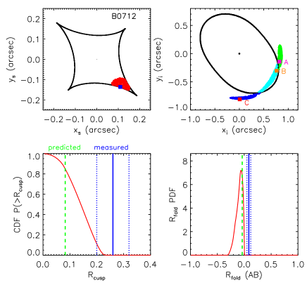
Figure 5: An example of the diagnostic plots, made for B0712$+$472, in the absence of CDM substructures. Top panels: the tangential caustic and critical curve from the best-fit lens model. Observed image positions of the close triplet (A, B, C) are plotted as squares in the image plane (on the right), the predicted source position is plotted as square in the source plane (on the left). $1.5\times 10^{6}$ source positions around the predicted source position are plotted in red, the corresponding close triple images are plotted in green, cyan and blue. Bottom panels: cumulative probability of $R_{\rm cusp}$ larger than a given value and the probability distribution function of $R_{\rm fold}$; measured and predicted flux ratios are indicated with blue and green lines, respectively. Blue dotted lines indicate error on the measurements.

Fig.5 gives an example of the diagnostic plots, made for B0712$+$472, in the absence of CDM substructures. Top panels show the tangential caustic and critical curve from the best-fit lens model; observed image positions of the close triplet are plotted in the image plane, and the corresponding source position is plotted in the source plane. $1.5\times 10^{6}$ source positions around the predicted source position are generated, and the corresponding close triple images are found. The bottom panels present the cumulative probability for $R_{\rm cusp}$ to be larger than a given value for the close image triplet and the probability distribution function of $R_{\rm fold}$ for the closest saddle-minimum image pair.

It is important to note that the cumulative probability of $R_{\rm cusp}$ does not drop sharply from 1.0 to 0.0 around the model predicted $R_{\rm cusp}$, due to the non-local effect resulting from including a wider range of source positions.

To select realizations that better resemble the observed systems, we have applied stricter criteria on the image configuration parameters $\Delta\phi$, $\theta/\theta_{\rm Ein}$ and $\theta_{1}/\theta_{2}$ of each simulated system, where $\theta_{2}$ is the distance between the second closest image pairs in the triplet configuration. We require the relative differences between the simulated and the observed quantities to be no larger than 10%:

$$\left\{\begin{array}[]{c}\bigg{|}\frac{(\Delta\phi)_{\rm sim}}{(\Delta\phi)_{\rm obs}}-1\bigg{|}\leqslant 10\%,\\ \bigg{|}\frac{(\theta/\theta_{\rm Ein})_{\rm sim}}{(\theta/\theta_{\rm Ein})_{\rm obs}}-1\bigg{|}\leqslant 10\%,\\ \bigg{|}\frac{(\theta_{1}/\theta_{2})_{\rm sim}}{(\theta_{1}/\theta_{2})_{\rm obs}}-1\bigg{|}\leqslant 10\%.\end{array}\right.$$ (5)

The choice of 10% is arbitrary. We are aiming at only selecting systems that most resemble the observed ones but also having enough realizations to be statistically significant. The choice of 10% results in at least $2\times 10^{4}$ realizations for each of the eight observed lenses, and the probability distribution functions for $R_{\rm cusp}$ and $R_{\rm fold}$ would not change much if using 20% instead of 10%.

There are two main advantages from studying individual systems via using their specific image configurations and their own lens models (plus CDM substructures). First, it gives us a handle to compensate for magnification bias to a certain level. Second, it may help us to identify other possible sources for flux anomalies apart from density perturbations due to substructures. Below we present results for each individual system.

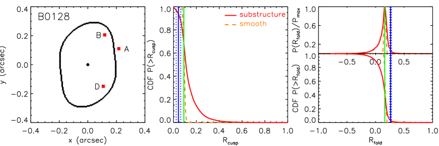
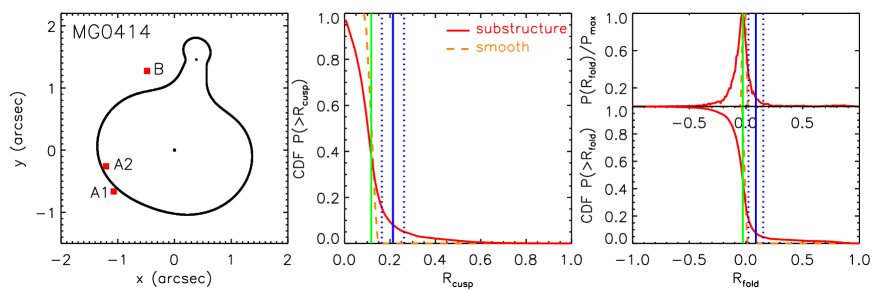
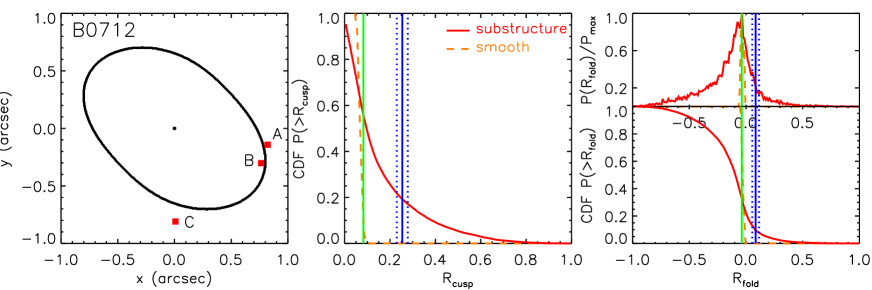
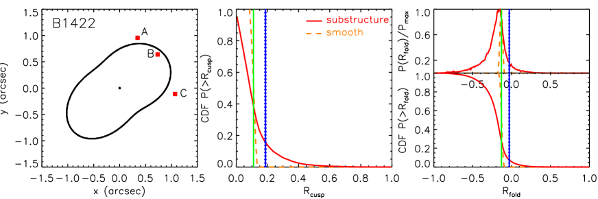
Figure 6: Diagnostic plots for B0128, MG0414, B0712 and B1422, after applying further criteria to select realizations that most resemble the observed image configurations. Left panel: critical curves and observed image positions; middle panel: cumulative probability distribution functions of $R_{\rm cusp}$; right panel: cumulative and probability distribution functions for $R_{\rm fold}$. Orange dashed lines indicate the distribution functions calculated under macro lens models in the absence of CDM substructures; red solid lines indicate those after adding CDM substructures. Measured and predicted flux ratios are indicated in blue and green lines, respectively. Blue dotted lines indicate error on the measurements.

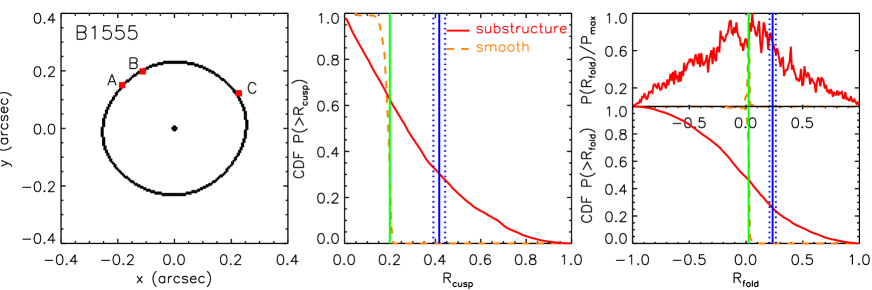
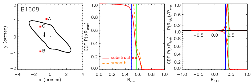
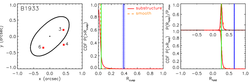
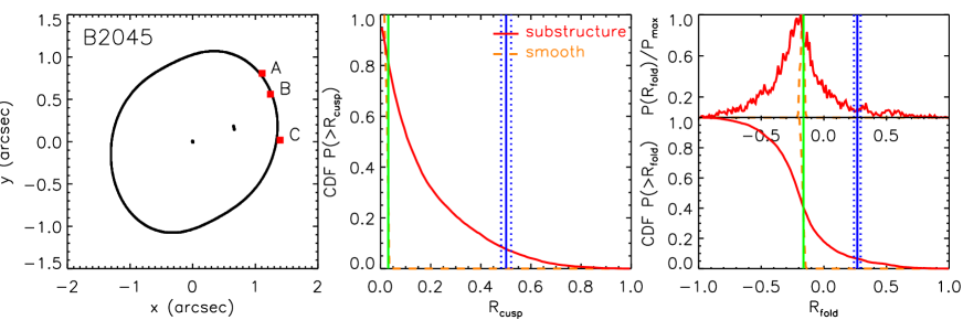
Figure 7: Same as Fig.6 but for B1555, B1608, B1933 and B2045.

5.2.1 B0128+437

The observed flux ratios are likely affected by complex systematic errors, as suggested by radio-frequency dependent flux ratios and by VLBI imaging. The VLBI data show that the source is composed of three aligned components, one being tentatively associated with a flat spectrum core and the other two with steep spectrum components of the jet. The lensed image $B$ only barely shows the “triple” structures, which are visible in image $A$, $C$ and $D$. Hence it is likely that image $B$ is affected by scatter broadening (Biggs et al. 2004). On the other hand, lens modelling using the VLBI data also suggests astrometric perturbation of image positions by substructures (Biggs et al. 2004).

Despite of these uncertainties affecting the observed flux ratios, B0128 is not an outlier of both $R_{\rm cusp}$ and $|R_{\rm fold}|$ distributions under smooth general lens models. However, our specific lens modelling indicates that the measured and predicted $R_{\rm fold}$ are incompatible within the measurement error. This discrepancy is less likely to be caused by density perturbations from substructures as the image pairs are located relatively far from the critical curve (image magnifications $|\mu|<10$), but could be related to the above mentioned systematic errors that affect the observed flux ratios, or due to simplified lens modelling.

5.2.2 MG0414+0534

MG0414+0534 is a fold system with a pair of images close to the critical curve (image magnifications $|\mu|>15$). The low-resolution radio observations of Lawrence et al. (1995) lead to roughly the same $R_{\rm cusp}=0.36$ at epochs separated by several months and at different frequencies from 5Ghz to 22 Ghz with the VLA, suggesting that the time delay between the lensed images is not a concern. However, a lower value of $R_{\rm cusp}=0.213$ was obtained from higher-resolution VLBI observations of Ros et al. (2000), which resolved the core+jet components of the source. The flux ratios from VLBI for the core images also agree well with the MIR flux ratios (Minezaki et al. 2009). The $R_{\rm fold}$ values from VLA, VLBI, MIR and extinction-corrected optical data all agree with each other within the measurement uncertainties. We use the VLBI results in both $R_{\rm cusp}$ and $R_{\rm fold}$ for our analysis.

MG0414 is not an outlier of either $R_{\rm cusp}$ or $|R_{\rm fold}|$ distributions predicted by general lens models in the absence of CDM substructures. However, specific lens modelling reveals inconsistency between the measurements and model predictions. Again the large image magnifications suggest the possibility for the flux ratios to be (easily) affected by local density perturbations. It can be seen that after adding CDM substructures to the macro lens model of this system (Fig.7), there is a probability of $\sim 10\%$ to have $R_{\rm cusp}$ and $R_{\rm fold}$ larger than the observed values. Interestingly, MacLeod et al. (2012) have also shown that the flux ratios between images $A1$ and $A2$ could be reproduced by adding a substructure of $\sim 10^{7}M_{\sun}$ close to image $A2$. Combining all these pieces of evidence above, CDM substructures are highly likely to be responsible for the observed flux anomalies in this system.

5.2.3 B0712+472

B0712+472 is a cusp/fold system with a close image configuration of $\Delta\phi=76.9^{\circ}$. The radio flux ratios seem relatively constant over time and radio frequencies (Jackson et al. 2000, Koopmans et al. 2003) but deviate significantly from the optical/NIR flux ratios, which are affected by differential extinction and microlensing (Jackson et al. 1998, 2000). This system shows discrepancies between the observed and model predicted $R_{\rm cusp}$ and $R_{\rm fold}$. Using general lens models, B0712 is an outlier of the $R_{\rm cusp}$ probability distributions in the absence of substructures.

From Fig.6 it can be seen that the probabilities to have $R_{\rm cusp}$ and $R_{\rm fold}$ larger than the observed values are 20% and 10%, respectively, again consistent with the statistical result from Sect.4. This is strong evidence for CDM substructures to be at least partly responsible for the observed flux anomalies.

On the other hand, the lens environment might also impact the flux ratios. Indeed, a galaxy group has been identified on the line of sight towards that system (Fassnacht & Lubin 2002, Fassnacht et al. 2008). We were unsuccessful in accounting for this group in the smooth lens model (Table 2) due to its uncertain X-ray centroid. A more detailed study of the lens environment in this system is needed to estimate its effect on the flux ratios.

5.2.4 B1422+231

B1422+231 is a classical cusp lens with $\Delta\phi=77^{\circ}$. The flux ratios measured at different radio frequencies and at different epochs and with different spatial resolution all agree with each other, as well as with mid-infrared (MIR) data (Patnaik et al. 1992, 1999; Koopmans et al. 2003; Chiba et al. 2005). Hence, the observed values of $R_{\rm cusp}$ and $R_{\rm fold}$ are robustly determined. As Keeton et al. (2003) pointed out, this system is not an outlier of the flux-ratio probability distributions using general lens models in the absence of CDM substructures. This can be seen again from the top panel of our Fig.2. However, discrepancies (larger than the measurement uncertainty) exist between measurements and best-fit model predictions for both $R_{\rm cusp}$ of the close triple image $A$, $B$ and $C$, and $R_{\rm fold}$ of the closest image pair $A$ and $B$ (but not for the second closest pair $B$ and $C$).

From Fig.6 we can see that the probability of $R_{\rm cusp}$ ($R_{\rm fold}$) larger than the observed value is 15% (10%) in the presence of CDM substructures, which is consistent with the statistical result from Sect.4 and with previous analysis of the flux ratios by Bradač et al. (2002). The discrepancy between the measured and the predicted flux ratios are therefore very likely to be caused by density fluctuations from CDM substructures around image $A$, which is also consistent with Dobler & Keeton (2006) using detailed lens modelling.

5.2.5 B1555+375

B1555+375 is a fold system, with a pair of images predicted to be very close to the critical curve (image magnifications $|\mu|>50$). Specific lens modellings indicate discrepancies between the observed and model predicted $R_{\rm cusp}$ and $R_{\rm fold}$ (here and also e.g., Keeton et al. 2003, 2005). As discussed in Sect.4, generic cusp and fold probability distributions would classify this system as an outlier, even in the presence of CDM substructures.

Considering the large image magnifications, the flux ratios could be easily affected by local density perturbations. Through specific lens modelling in the presence of CDM substructures, the probabilities reach as high as $\sim 30\%$ for $R_{\rm cusp}$ and $R_{\rm fold}$ larger than the observed values (see Fig.6). It is highly likely that substructures are responsible for the discrepancies between measurements and model predictions in this system.

We caution that the lens model however, might not be optimal as the position angles of the ellipticity and of the external shear are nearly orthogonal. The HST images of this system also suggest that it is a very flattened lens. All these strongly indicate a possibly missing ingredient in the lens model. Higher resolution radio images (only MERLIN data are currently available) as well as deep optical imaging and spectroscopy are needed for a better characterization to this system in order to draw firm conclusions about the macro lens model.

5.2.6 B1608+656

Many VLA data are available (including monitoring data) for this system and show consistently $R_{\rm fold}\sim 0.32$. The radio measurements of $R_{\rm cusp}$ and $R_{\rm fold}$ are larger than observed in the optical and NIR, where the source appears to be extended and significantly affected by differential extinction (Surpi & Blandford 2003).

For this system, both measured $R_{\rm cusp}$ and $R_{\rm fold}$ are smaller than model predictions. As all three images in the close triplet are located far away from the critical curve ($|\mu|<5$), we do not expect significant magnification variation caused by local density perturbations from CDM substructures. The main lens of B1608 is confirmed to be a spiral galaxy (Fassnacht et al. 1996). Such a system may host a massive disc component, which is not accommodated by our model but could affect flux ratios (Maller et al. 2000; Möller et al. 2003).

5.2.7 B1933+503

B1933+503 is also a fold system, showing discrepancies between the observed and model predicted $R_{\rm cusp}$ and $R_{\rm fold}$. The VLBI images presented in Suyu et al. (2012) reveal that the cores in images 1 and 4 show two peaks but not for image 3. This suggests that scatter broadening may modify the radio flux ratios. The $R_{\rm cusp}$ and $R_{\rm fold}$ obtained from this high resolution images also agree with lower resolution VLA and MERLIN data (Sykes et al. 1998).

On the other hand, all three images in the close triplet are located far away from the critical curve ($|\mu|<5$), such that we do not expect local density perturbations from CDM substructures to be responsible for the observed flux anomalies. This can also be seen from Fig.7, where CDM substructures can do almost nothing to increase the probability for the observed flux ratios for this system.

Overall, it seems that the uncertainties on the observed flux ratios and the use of a too simplified macro model (as suggested by a $\chi^{2}=4.7$, from our Table 2) may account for the anomalies in this system.

5.2.8 B2045+265

B2045+265 is a very extreme cusp lens with $\Delta\phi=34.9^{\circ}$. All three images are located (symmetrically) close to the critical curve with image magnifications $|\mu|>50$. The radio flux ratios are very robust at different spatial resolution (VLA, VLBA) over different periods of time, and consistent with the H-K wavelengths (Fassnacht et al. 1999, McKean et al. 2007). Koopmans (2003) identified significant intrinsic variability at radio wavelengths, but the amplitude of this effect is apparently small, at least on time scale of months. This lens shows flux anomalies in both $R_{\rm cusp}$ and $R_{\rm fold}$ through specific lens modelling. The VLBA data reveals a core+jet emission for image $A$, but not for the saddle point image $B$, which should be brighter than $A$ according to the models. This indicates a possibility of the presence of a substructure around image $B$ that demagnifies both the compact core and jet emissions.

Same as for B1555, this system would be an outlier of generic cusp and fold probability distributions, even in the presence of CDM substructures (see Sect.4). But the close configuration and large image magnifications suggest that the flux ratios can be easily affected by density perturbations from substructures. This can be seen clearly after adding CDM substructures to the best-fit lens potential of this system (Fig.7), the probabilities now reach $\sim 10\%$ for $R_{\rm cusp}$ and $R_{\rm fold}$ to be larger than the observed values.

5.3 Selection and magnification effects

The flux-ratio probability distributions presented in Fig.6 and 7 are calculated for realizations with image configurations that satisfy Eq.5. As the true selection function is hard to quantify and thus take into account, we caution that the statistical results may change if the sample is selected using different criteria. Here we investigate the flux-ratio probability distributions for realizations selected according to image magnification instead of image configuration.

The final statistics are very different for B0712, B1422 and B2045; but no significant differences are seen for the rest five systems, as for which, the magnification selection does not lead to a realization sample that is very different from using image configuration selection. Fig.8 presents the $R_{\rm cusp}$ probability distributions using two different criteria to select systems that most resemble the three systems above. In particular, the solid curves are for realizations whose saddle image magnifications $|\mu_{\rm sad}|\geqslant 20,~{}15~{}{\rm and}~{}70$, which are model predictions for B0712, B1422 and B2045, respectively.

It can be seen clearly that using realizations selected according to magnification criteria results in higher probabilities to have $R_{\rm cusp}$ as large as measurements. As a matter of fact, as the applied magnification cut goes up, such probabilities will increase accordingly. This again reflects the fact that images close to the critical curves thus having large magnifications, are more likely to be affected by substructures and thus show larger $R_{\rm cusp}$. Using magnification selection criteria, the probabilities for these three systems become $20\%\sim 30\%$, which again highly suggest that CDM substructures are responsible for the observed flux ratio anomalies therein.

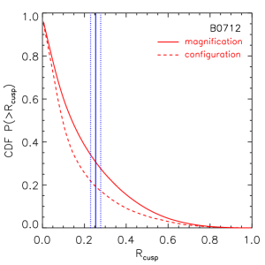
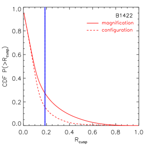
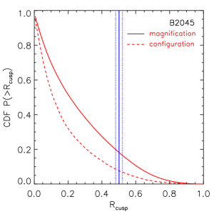
Figure 8: Cumulative distribution functions of $P(>R_{\rm cusp})$ for system B0712, B1422 and B2045. Dashed curves are for realizations selected according to image configurations that satisfy Eq.5; solid curves are for realizations whose saddle image magnifications are no less than those in B1422, B0712 and B2045. The blue vertical lines indicate the measured $R_{\rm cusp}$ with error bars.

6 DISCUSSION AND CONCLUSIONS

Discrepancies between the observed and model-predicted flux ratios in $R_{\rm cusp}$ and $R_{\rm fold}$ are seen in a number of radio lenses. The interpretation of these anomalies is that substructures present in lensing galaxies perturb the lens potentials and alter image magnifications (and thus flux ratios). These systems have therefore been used to constrain the subhalo abundance predicted in the CDM model of structure formation. Our previous studies (Xu et al. 2009 and 2010) found that the number of subhalos in high-resolution simulation of galactic CDM halos is insufficient to account for the observed frequency of flux anomalies.

However, our previous work suffered from three shortcomings: (1) We had access to only six high-resolution simulations which we projected along a small number of directions; halo-to-halo variations in the subhalo population and its projected spatial distribution could have led to biased results; (2) Our main lens models assumed relatively small ellipticities (axis ratios $q=0.8$) instead of the full range and this too could have resulted in flawed conclusions; (3) Most importantly, using the subhalo populations in $N$-body simulations of Milky Way-sized halos could have underestimated the flux anomaly frequency caused by the more abundant subhalo populations of group-sized halos, which are more likely to host the observed massive elliptical lenses.

In the first part of this work, we have attempted to overcome these shortcomings and establish whether or not CDM substructures can account for the flux ratio anomalies observed in the best currently available sample of quasars (see Table 1), nearly all of which show discrepancies between the measured $R_{\rm cusp}$ (and $R_{\rm fold}$) and those predicted by best-fit smooth models. We assume that the general smooth lens potentials can be modelled as isothermal ellipsoids with a wide range of axis ratios, higher-order multipole perturbations and randomly oriented external shear (Sect.3.1). We have analyzed two sets of state-of-the-art high resolution CDM cosmological simulations: the Aquarius suite of galactic halos and the Phoenix suite of cluster halos whose subhalo populations are rescaled to those expected in group-sized halos (Sect.3.2).

We find that each of the three shortcomings of our previous work can indeed lead to biased results. Firstly, a limited number of halo projections fails to fairly sample relatively massive subhalos. When a large number of projections are used instead the true spatial distributions are recovered in the inner parts of the host halos (Fig.3). Secondly, when a wide range of ellipticities are considered, larger flux ratios in $R_{\rm cusp}$ and $|R_{\rm fold}|$ are obtained even without the presence of substructures (Sect.4.2; also Keeton et al. 2003 and 2005, Metcalf & Amara 2012). Thirdly, the richer subhalo populations of group-sized halos result in significantly higher flux anomaly probabilities (Figs.2 and 4 and Sect.4). We now estimate the surface mass fraction in subhalos (in group-sized halos) within or around the tangential critical curve to be $\sim 1\%$ instead of 0.3% as in Xu et al. (2009).

Using a generalized smooth lens population plus subhalos hosted by group-sized halos we show in our Fig.2 and Sect.4 that substructures do not strongly change the flux-ratio probability distributions for image triplets or pairs with large separations; by contrast, for small separations the distributions are significantly affected, resulting in a substantial amount of flux-ratio variations (the anomalies). This is expected from the magnification behavior $\mu\approx(1-2\kappa)^{-1}$, and thus $\delta\mu/\mu\propto\mu\delta\kappa$; at around the critical curves, $\mu\rightarrow\infty$. As a result, a tiny density fluctuation near an image position that is close to the critical curve will significantly perturb the local image magnification; while a density fluctuation around an image that is further away from the critical curve will be far less efficient in altering the image magnification via density perturbation. For this reason, image triplets and pairs with small separations are best probes of substructure abundance in lensing galaxies.

The application of generic smooth lens potentials, however, has its limitations in at least the following two aspects: (1) without allowing for secondary lenses in the field, it cannot model systems with complex lens environments from e.g., satellite galaxies or nearby galaxy groups/clusters; (2) without considering magnification effects, it cannot fairly sample systems with extreme image configurations, for which although the corresponding source positions only occupy a tiny fraction of the region inside the caustic in the source plane, such rare events would be among the brightest detections in the Universe due to huge magnification effect.

To compensate for these limitations, in the second part of this work, we have added CDM substructures to the model-predicted specific lens potentials of individual systems in our sample and studied the perturbation effects of substructures in the observed specific image configurations; results are given in Table 2, Fig.6 and 7 in Sect.5.

We have also qualitatively investigated the effect of magnifications by applying different image magnification cuts, and compared the results between realizations selected using magnifications cuts and using configuration criteria (in Sect.5.3). We found that the higher the applied magnification cut is, the larger probability there is for the realization sample to have large $R_{\rm cusp}$, this again is because of the behavior of the magnification perturbation: $\delta\mu/\mu\propto\mu\delta\kappa$ around the critical curve.

Among the eight lenses in our sample, B1422, B0712, B1555, B2045 and MG0414 have image triplets or pairs with small separations, indicated by image magnifications $|\mu|>15$. For these systems, we find that the probability of obtaining the observed flux ratios as a result of perturbations by subhalos in group-sized halos are $20\%\sim 30\%$, strongly suggesting that CDM substructures can account for a non-negligible amount of the observed flux-ratio anomalies. This demonstrates that lensed quasars are very good probes of substructures in distant early-type galaxies, complementary to lensed galaxies showing surface brightness variations (Vegetti & Koopmans 2009; Vegetti et al. 2010, 2012).

It is important to bear in mind that, in addition to substructures within the halo of the lensing galaxy, objects along the line-of-sight to the lensed quasar can also perturb the lens potential and give rise to flux-ratio anomalies (Chen et al. 2003; Wambsganss et al. 2005; Puchwein & Hilbert 2009). The contribution of these interlopers can be as important as that of the intrinsic substructures within the lensing galaxy (e.g. Metcalf, 2005a, b; Miranda & Macciò, 2007; Xu et al., 2012).

Finally for systems with large close-pair image separations, e.g., B1933 in our sample (with image magnifications $|\mu|<5$), the observed flux-ratio discrepancies (between the observed and model-predicted) are unlikely due to substructure density perturbations. Instead we attribute them either to light propagation effects in the interstellar medium or to inaccuracies in simplified smooth lens models. Here we make a bold prediction that applying standard lens modelling techniques (e.g., as practiced here) to state-of-the-art hydrodynamic simulations, in which interaction between baryons and dark matter are taken into account, will reveal a good fraction flux-ratio anomalies in systems with large close-pair separations.

Appendix A Summary of the best flux ratios for the sample of lensed systems

We provide in Table  3 the best available flux ratio measurements for the sample of lenses studied in the main text. When flux ratios vary with spatial resolution due to resolved structures in images, we provide measurements obtained at different spatial resolution. When available, we also report flux ratios averaged over several epochs or corrected for time delays between images. In Table  3, VLBA and VLBI images have typical beam sizes of 2 ${\rm mas}^{2}$ while VLA and MERLIN frames have typical beam sizes of 50 ${\rm mas}^{2}$.

Table 3: Observed lenses with measurements of $R_{\rm cusp}$ and $R_{\rm fold}$ for the close triple images:

ID	Observation	$F_{1}$	$F_{2}$	$F_{3}$	$R_{\rm cusp}$	${R_{\rm fold}}$	Image name	References
B0128$\dagger$	VLA 5 Ghz 41 epochs	0.584$\pm$0.029	1.0$\pm$0.0	0.506$\pm$0.032	0.043$\pm$0.020	0.263$\pm$0.014	B*-A-D*	1
	VLBA 5 Ghz	2.8$\pm$0.28	10.6$\pm$1.06	4.8$\pm$0.48	0.165$\pm$0.055	0.582$\pm$0.034	-	2
	Merlin 5 Ghz	9.5$\pm$1	18.9$\pm$1	9.2$\pm$1	0.005$\pm$0.046	0.331$\pm$0.033	-	3
MG0414	VLBI 8.5 Ghz core	115.6$\pm$11.56	97$\pm$9.7	34$\pm$3.4	0.213$\pm$0.049	0.087$\pm$0.065	A1-A2*-B	4
	VLA 15 Ghz 4 epochs	157.0$\pm$5.5	138.75$\pm$5	138.75$\pm$2.25	0.361$\pm$0.012	0.062$\pm$0.024	-	5
	MIR	1.0$\pm$0.0	0.9$\pm$0.04	0.36$\pm$0.02	0.204$\pm$0.016	0.053$\pm$0.020	-	6
B0712	VLA 5 Ghz 41 epoch	1.0$\pm$0.0	0.843$\pm$0.061	0.418$\pm$0.037	0.254$\pm$0.024	0.085$\pm$0.030	A-B*-C	1
	VLBA 5 Ghz	10.7$\pm$0.15	8.8$\pm$0.15	3.6$\pm$0.15	0.238$\pm$0.009	0.097$\pm$0.010	-	7
B1422	VLA 5 Ghz 41 epochs	1.0$\pm$0.0	1.062$\pm$0.009	0.551$\pm$0.007	0.187$\pm$0.004	-0.030$\pm$0.004	A-B*-C	1
	VLBA 8.4 Ghz	152$\pm$2	164$\pm$2	81$\pm$1	0.174$\pm$0.006	-0.038$\pm$0.009	-	8
B1555	VLA 5 Ghz 41 epochs	1.0$\pm$0.0	0.62$\pm$0.059	0.507$\pm$0.073	0.417$\pm$0.026	0.235$\pm$0.028	A-B*-C	1
B1608$\dagger\dagger$	VLA 8.5 Ghz	2.045$\pm$0.01	1.037$\pm$0.01	1.0$\pm$0.001	0.492$\pm$0.002	0.327$\pm$0.003	A-C*-B	9
B1933$\dagger$	VLBA 5 Ghz	4.7$\pm$0.4	19.4$\pm$0.4	5.4$\pm$0.4	0.315$\pm$0.016	0.610$\pm$0.009	3*-4-6*	10
	VLA 15 Ghz	2.5$\pm$0.4	15.5$\pm$0.4	3.2$\pm$0.4	0.462$\pm$0.018	0.722$\pm$0.009	-	10
B2045	VLA 5 Ghz 41 epochs	1.0$\pm$0.0	0.578$\pm$0.059	0.739$\pm$0.073	0.501$\pm$0.020	0.267$\pm$0.027	A-B*-C	1
	VLBA 5 Ghz	1.0$\pm$0.01	0.61$\pm$0.01	0.93$\pm$0.01	0.520$\pm$0.003	0.242$\pm$0.007	-	11

Notes: ($\dagger$) Flux ratios are likely affected by systematic errors due to scattering. ($\dagger\dagger$) Quoted fluxes are after correction for the time delays. In the table, fluxes and errors (in Col.3, 4 and 5) are directly taken from literatures in their original units. When flux errors are not available, we take 10% of the measured fluxes as their uncertainties. Image names (in Col.8) associated with * indicate the images have negative parities. References (1) Koopmans et al. 2003; (2) Biggs et al. 2004 (Table 3); (3) Phillips et al. 2000; (4) Ros et al. 2000; (5) Lawrence et al. 1995; (6) Minezaki et al. 2009; (7) Jackson et al. 2000; (8) Patnaik et al. 1999; (9) Fassnacht et al. 1999; (10) Sykes et al. 1998; (11) McKean et al. 2007.

Appendix B Generalized isothermal lens with multipole perturbation and external shear

Consider a lens potential composed of a singular isothermal ellipsoidal, $m^{\rm th}$-mode multipole perturbation and external shear:

$$\psi(\theta,\phi)=\psi_{\rm SIE}(\theta,\phi)+\psi_{m}(\theta,\phi)+\psi_{\rm ext}(\theta,\phi)$$ (6)

where $\theta$ and $\phi$ are the image position $\vec{\theta}$=($\theta_{x}$, $\theta_{y}$) in polar coordinate: $\theta=\sqrt{\theta_{x}^{2}+\theta_{y}^{2}}$ and $\phi=\tan^{-1}(\theta_{y}/\theta_{x})$; $\psi_{\rm SIE}$, $\psi_{m}$ and $\psi_{\rm ext}$ are lens potentials of an singular isothermal ellipsoidal, $m^{\rm th}$-mode multipole perturbation and external shear, respectively. The deflection angles and second-order derivatives of the total lens potential are then given by:

$$\left\{\begin{array}[]{l}\alpha_{x}(\theta,\phi)\equiv\frac{\partial\psi}{\partial\theta_{x}}=\alpha_{\textrm{SIE},x}(\theta,\phi)+\alpha_{m,x}(\theta,\phi)+\alpha_{\textrm{ext},x}(\theta,\phi)\\ {}{}\\ \alpha_{y}(\theta,\phi)\equiv\frac{\partial\psi}{\partial\theta_{y}}=\alpha_{\textrm{SIE},y}(\theta,\phi)+\alpha_{m,y}(\theta,\phi)+\alpha_{\textrm{ext},y}(\theta,\phi)\\ {}{}\\ \psi_{11}(\theta,\phi)\equiv\frac{\partial^{2}\psi}{\partial\theta_{x}^{2}}=\psi_{\textrm{SIE},11}(\theta,\phi)+\psi_{m,11}(\theta,\phi)+\psi_{\textrm{ext},11}(\theta,\phi)\\ {}{}\\ \psi_{22}(\theta,\phi)\equiv\frac{\partial^{2}\psi}{\partial\theta_{y}^{2}}=\psi_{\textrm{SIE},22}(\theta,\phi)+\psi_{m,22}(\theta,\phi)+\psi_{\textrm{ext},22}(\theta,\phi)\\ {}{}\\ \psi_{12}(\theta,\phi)\equiv\frac{\partial^{2}\psi}{\partial\theta_{x}\theta_{y}}=\psi_{\textrm{SIE},12}(\theta,\phi)+\psi_{m,12}(\theta,\phi)+\psi_{\textrm{ext},12}(\theta,\phi).\end{array}\right.$$ (7)

In our numerical approach for lensing calculations, we tabulate to a Cartesian mesh ($\theta_{x}$, $\theta_{y}$) in the image plane values of the reduced deflection angle and second-order derivatives of the lens potential. Here below we give the exact analytical formulae for the lensing quantities in Eq.7.

For generalized isothermal lens (plus perturbation), the lens potential $\psi$ and convergence $\kappa$ follow the pair equations below (Keeton et al. 2003, Appendix B2):

$$\left\{\begin{array}[]{l}\psi(\theta,\phi)=\theta F(\phi)=\theta[F_{\rm SIE}(\phi)+\sum\limits_{m=3,4}F_{m}(\phi)]\\ {}{}\\ \kappa(\theta,\phi)=R(\phi)[2\theta]^{-1}=[R_{\rm SIE}(\phi)+\sum\limits_{m=3,4}\delta R_{m}(\phi)][2\theta]^{-1}.\end{array}\right.$$ (11)

From the Poisson equation $\nabla^{2}\psi=2\kappa$, $F(\phi)$ and $R(\phi)$ are related by: $R(\phi)=F(\phi)+F^{\prime\prime}(\phi)$. $F_{\rm SIE}(\phi)$ and $R_{\rm SIE}(\phi)$ are shape functions of a singular isothermal ellipsoidal lens, while $F_{m}(\phi)$ and $\delta R_{m}(\phi)$ describe the higher-order multipole perturbations. For the generic lens model used in this work, only $m=3$ and 4 are considered.

B.1 Singular isothermal ellipsoidal

Specifically, if the isothermal ellipsoidal’s major and minor axes coincide with the Cartesian axes, then the shape functions are given by (Kassiola & Kovner 1993; Kormann, Schneider & Bartelmann 1994; Keeton & Kochanek 1998):

$$\left\{\begin{array}[]{l}R_{\rm SIE}(\phi)=\frac{\theta_{\rm Ein}}{\sqrt{1-\epsilon\cos 2\phi}}\\ {}{}\\ F_{\rm SIE}(\phi)=\frac{\theta_{\rm Ein}}{\sqrt{2\epsilon}}\bigg{[}\cos\phi\tan^{-1}\bigg{(}\frac{\sqrt{2\epsilon}\cos\phi}{\sqrt{1-\epsilon\cos 2\phi}}\bigg{)}+\sin\phi\tanh^{-1}\bigg{(}\frac{\sqrt{2\epsilon}\sin\phi}{\sqrt{1-\epsilon\cos 2\phi}}\bigg{)}\bigg{]}.\end{array}\right.$$ (12)

where $\theta_{\rm Ein}$ is the Einstein radius of the singular isothermal ellipsoidal, $\epsilon=(1-q^{2})/(1+q^{2})$ and $q\in(0,1]$ is the axis ratio of the ellipsoidal. It can be shown that $R_{\rm SIE}(\phi)$ is the equation in polar coordinates of the ellipse at the critical curve, where $\kappa_{\rm SIE}=\frac{1}{2}$. $R_{\rm SIE}(\phi)$ corresponds to the ellipse’s equation in Cartesian coordinates:

$$\frac{\theta_{x}^{2}}{a^{2}}+\frac{\theta_{y}^{2}}{b^{2}}=1,~{}\textrm{where~{}~{}}a=\frac{\theta_{\rm Ein}}{\sqrt{1-\epsilon}},~{}b=aq=\frac{\theta_{\rm Ein}}{\sqrt{1+\epsilon}}.$$ (13)

As convergence $\kappa_{\rm SIE}(\theta,\phi)=\frac{R_{\rm SIE}(\phi)}{2\theta}$, the iso-$\kappa_{\rm SIE}$ contours follow the ellipse $R_{\rm SIE}(\phi)$ and are scaled by $\theta^{-1}$. The deflection angles are given by (e.g., Keeton & Kochanek 1998):

$$\left\{\begin{array}[]{l}\alpha_{\textrm{SIE},x}(\theta,\phi)=\frac{\theta_{\rm Ein}}{\sqrt{2\epsilon}}\tan^{-1}(\frac{\sqrt{2\epsilon}\cos\phi}{\sqrt{1-\epsilon\cos 2\phi}})\\ {}{}\\ \alpha_{\textrm{SIE},y}(\theta,\phi)=\frac{\theta_{\rm Ein}}{\sqrt{2\epsilon}}\tanh^{-1}(\frac{\sqrt{2\epsilon}\sin\phi}{\sqrt{1-\epsilon\cos 2\phi}}).\end{array}\right.$$ (14)

The second-order derivatives are given by:

$$\left\{\begin{array}[]{l}\psi_{\textrm{SIE},11}(\theta,\phi)=\frac{\theta_{\rm Ein}\sin^{2}\phi}{\theta\sqrt{1-\epsilon\cos 2\phi}}\\ {}{}\\ \psi_{\textrm{SIE},22}(\theta,\phi)=\frac{\theta_{\rm Ein}\cos^{2}\phi}{\theta\sqrt{1-\epsilon\cos 2\phi}}\\ {}{}\\ \psi_{\textrm{SIE},12}(\theta,\phi)=-\frac{\theta_{\rm Ein}\sin\phi\cos\phi}{\theta\sqrt{1-\epsilon\cos 2\phi}}.\end{array}\right.$$ (15)

B.2 System rotation

If the major axis of the isothermal ellipse is not aligned with the $x$-axis, but with a position angle of $\phi_{\rm rot}$, then an image position ($\theta,\delta$), where $\delta$ is the position angle measured from the (positive) major axis of the isothermal ellipse, after rotation will become ($\theta,\phi$) in the new polar coordinates, where $\phi=\delta+\phi_{\rm rot}$. The transformation of the lensing properties between the two systems before and after rotation is described by:

$$\left\{\begin{array}[]{l}\alpha_{x}(\theta,\phi)=\widetilde{\alpha_{x}}(\theta,\delta)\cos\phi_{\rm rot}-\widetilde{\alpha_{y}}(\theta,\delta)\sin\phi_{\rm rot}\\ {}{}\\ \alpha_{y}(\theta,\phi)=\widetilde{\alpha_{x}}(\theta,\delta)\sin\phi_{\rm rot}+\widetilde{\alpha_{y}}(\theta,\delta)\cos\phi_{\rm rot}\\ {}{}\\ \psi_{11}(\theta,\phi)=\cos^{2}\phi_{\rm rot}\widetilde{\psi_{11}}(\theta,\delta)+\sin^{2}\phi_{\rm rot}\widetilde{\psi_{22}}(\theta,\delta)-2\sin\phi_{\rm rot}\cos\phi_{\rm rot}\widetilde{\psi_{12}}(\theta,\delta)\\ {}{}\\ \psi_{22}(\theta,\phi)=\sin^{2}\phi_{\rm rot}\widetilde{\psi_{11}}(\theta,\delta)+\cos^{2}\phi_{\rm rot}\widetilde{\psi_{22}}(\theta,\delta)+2\sin\phi_{\rm rot}\cos\phi_{\rm rot}\widetilde{\psi_{12}}(\theta,\delta)\\ {}{}\\ \psi_{12}(\theta,\phi)=\sin\phi_{\rm rot}\cos\phi_{\rm rot}(\widetilde{\psi_{11}}(\theta,\delta)-\widetilde{\psi_{22}}(\theta,\delta))+(\cos^{2}\phi_{\rm rot}-\sin^{2}\phi_{\rm rot})\widetilde{\psi_{12}}(\theta,\delta)\end{array}\right.$$ (16)

where quantities on the left side of the equations are after rotation, those on the right and labeled with “$\sim$” are before rotation. As can be seen, the rotation transformation of the convergence $\kappa$ and shear $\gamma=\gamma_{1}+i\gamma_{2}$ in the two systems is then:

$$\left\{\begin{array}[]{l}\kappa(\theta,\phi)\equiv(\psi_{11}+\psi_{22})/2=\widetilde{\kappa}(\theta,\delta)\\ {}{}\\ \gamma_{1}(\theta,\phi)\equiv(\psi_{11}-\psi_{22})/2=\widetilde{\gamma_{1}}(\theta,\delta)\cos 2\phi_{\rm rot}-\widetilde{\gamma_{2}}(\theta,\delta)\sin 2\phi_{\rm rot}\\ {}{}\\ \gamma_{2}(\theta,\phi)\equiv(\psi_{12}+\psi_{21})/2=\widetilde{\gamma_{1}}(\theta,\delta)\sin 2\phi_{\rm rot}+\widetilde{\gamma_{2}}(\theta,\delta)\cos 2\phi_{\rm rot}.\end{array}\right.$$ (17)

In this work, we fix the major and minor axes of the isothermal ellipsoidal along the $x$- and $y$-axis, respectively, i.e., $\phi_{\rm rot}=0$. The derivations and equations given below are for this case; the orientations of the higher-order perturbation $\phi_{m}$ and external shear $\phi_{\rm ext}$ are both measured (counter-clockwise) from to the (positive) semi-major axis of the isothermal ellipsoidal.

B.3 Higher-order multipole perturbations

Now consider adding a higher-order multipole perturbation $\delta R_{m}(\phi)$ to the iso-$\kappa$ ellipse $R_{\rm SIE}(\phi)$, where $\delta R_{m}(\phi)$ is defined as (see Keeton et al. 2003, Appendix B2):

$$\delta R_{m}(\phi)=a_{m}^{\rm pert}\cos(m(\phi-\phi_{m}))$$ (18)

where $a_{m}^{\rm pert}$ ($>$0) and $\phi_{m}$ are the amplitude and “orientation” of the $m^{\rm th}$-order perturbation to the perfect ellipse $R_{\rm SIE}(\phi)$.

In a particular case for the 4^th-mode perturbation, an elliptical galaxy would be more disky if $\phi_{4}=0$, and more boxy if $\phi_{4}=\pi/4$ (which is the same as in the conventional definition that $\delta R_{4}(\phi)=a_{4}\cos(4\phi)$, where $a_{4}>0$ corresponds to a disky galaxy and $a_{4}<0$ corresponds to a boxy galaxy).

From Eq.11 it can be seen that, as convergence $\kappa(\theta,\phi)=[R_{\rm SIE}(\phi)+\Sigma\delta R_{m}(\phi)][2\theta]^{-1}$, now the new iso-$\kappa$ contours follow the perturbed ellipse $[R_{\rm SIE}(\phi)+\Sigma\delta R_{m}(\phi)]$ (at $\kappa=\frac{1}{2}$) and are scaled by $\theta^{-1}$.

The corresponding shape function $F_{m}(\phi)$ is given by (see Keeton et al. 2003):

$$F_{m}(\phi)=\frac{1}{1-m^{2}}a_{m}^{\rm pert}\cos(m(\phi-\phi_{m})).$$ (19)

The deflection angles and second order derivatives of the potential due to the $m^{\rm th}$ perturbation are given by:

$$\left\{\begin{array}[]{l}\alpha_{m,x}(\theta,\phi)=F_{m}(\phi)\cos\phi-F^{\prime}_{m}(\phi)\sin\phi\\ {}{}\\ \alpha_{m,y}(\theta,\phi)=F_{m}(\phi)\sin\phi+F^{\prime}_{m}(\phi)\cos\phi\\ {}{}\\ \psi_{m,11}(\theta,\phi)=[\theta]^{-1}\sin^{2}\phi[F_{m}(\phi)+F^{\prime\prime}_{m}(\phi)]=[\theta]^{-1}\sin^{2}\phi\delta R_{m}(\phi)\\ {}{}\\ \psi_{m,22}(\theta,\phi)=[\theta]^{-1}\cos^{2}\phi[F_{m}(\phi)+F^{\prime\prime}_{m}(\phi)]=[\theta]^{-1}\cos^{2}\phi\delta R_{m}(\phi)\\ {}\\ \psi_{m,12}(\theta,\phi)=-[2\theta]^{-1}\sin 2\phi[F_{m}(\phi)+F^{\prime\prime}_{m}(\phi)]=-[2\theta]^{-1}\sin 2\phi\delta R_{m}(\phi)\end{array}\right.$$ (20)

where $F^{\prime}_{m}=\frac{\partial F_{m}}{\partial\phi}$ and $F^{\prime\prime}_{m}=\frac{\partial^{2}F_{m}}{\partial\phi^{2}}$.

The physical quantity of $\delta R_{m}$ in Eq.18 is the same as in Hao et al. (2006), where a slightly different definition is given:

$$\delta R_{m}(\phi)=a_{m}\cos(m\phi)+b_{m}\sin(m\phi).$$ (21)

In their work, they studied the isophote shapes of 847 galaxies and presented mean $a_{m}/a$ and $b_{m}/a$ ($a$ is the semi-major axis length of the perfect ellipse) for $m=3,~{}4$, and mean ellipticity $e(\equiv 1-q)$ of the ellipse, averaged within the Petrosian half-light radius. We use these values in our main lens modelling. Notice that Eq.21 can also be re-written as: $\delta R_{m}(\phi)=\sqrt{a_{m}^{2}+b_{m}^{2}}\cos(m(\phi-\phi_{m}))$, where $\phi_{m}=\frac{1}{m}\tan^{-1}(b_{m}/a_{m})\in\frac{1}{m}[0,2\pi)$. Comparing with Eq.18, it can be seen that:

$$\left\{\begin{array}[]{l}a_{m}^{\rm pert}=\sqrt{a_{m}^{2}+b_{m}^{2}}\equiv\sqrt{(a_{m}/a)^{2}+(b_{m}/a)^{2}}\times a_{\rm SIE},\\ {}{}\\ \phi_{m}=\frac{1}{m}\tan^{-1}(b_{m}/a_{m})\end{array}\right.$$ (22)

where $a_{m}^{\rm pert}$ is re-normalized at $\kappa=\frac{1}{2}$; $a_{\rm SIE}=\frac{\theta_{\rm Ein}}{\sqrt{1-\epsilon}}$ as given in Eq.13. Therefore the model parameters for higher-order perturbations ($m=3,~{}4$) can be fixed using observational samples (Hao et al. 2006).

B.4 Constant external shear

The lens potential $\psi^{\rm ext}(\theta,\phi)$ caused by a constant external shear is given by:

$$\psi_{\rm ext}(\theta,\phi)=-\frac{\gamma_{\rm ext}}{2}\theta^{2}\cos(2(\phi-\phi_{\rm ext}))$$ (23)

where $\gamma_{\rm ext}(>0)$ is the shear amplitude and $\phi_{\rm ext}\in[0,\pi)$ is the position angle of the shear mass, measured counter-clockwise from the semi-major axis of the isothermal ellipsoidal. External shear will not contribute to external convergence, i.e., $\kappa_{\rm ext}=0$. The deflection angle and second-order derivatives are given by:

$$\left\{\begin{array}[]{l}\alpha_{\textrm{ext},x}(\theta,\phi)=-\theta\gamma_{\rm ext}\cos(\phi-2\phi_{\rm ext})\\ {}{}\\ \alpha_{\textrm{ext},y}(\theta,\phi)=\theta\gamma_{\rm ext}\sin(\phi-2\phi_{\rm ext})\\ {}{}\\ \psi_{\textrm{ext},11}(\theta,\phi)=-\gamma_{\rm ext}\cos(2\phi_{\rm ext})\\ {}{}\\ \psi_{\textrm{ext},22}(\theta,\phi)=\gamma_{\rm ext}\cos(2\phi_{\rm ext})\\ {}{}\\ \psi_{\textrm{ext},12}(\theta,\phi)=-\gamma_{\rm ext}\sin(2\phi_{\rm ext}).\end{array}\right.$$ (24)

In this work, we assume random external shear orientation in each simulated lensing system.

References

- Amara et al. (2006) Amara A., Metcalf R. B., Cox T. J., Ostriker J. P., 2006, MNRAS, 367, 1367
- Benson et al. (2002) Benson A. J., Frenk C. S., Lacey C. G., Baugh C. M., Cole S., 2002, MNRAS, 333, 177
- Biggs et al. (2004) Biggs A. D., Browne I. W. A., Jackson N. J., York T., Norbury M. A., McKean J. P., Phillips P. M., 2004, MNRAS, 350, 949
- Biggs et al. (2000) Biggs A. D., Xanthopoulos E., Browne I. W. A., Koopmans L. V. E., Fassnacht C. D., 2000, MNRAS, 318, 73
- Blandford & Narayan (1986) Blandford R., Narayan R., 1986, ApJ, 310, 568
- Bradač et al. (2004) Bradač M., Schneider P., Lombardi M., Steinmetz M., Koopmans L. V. E., Navarro J. F., 2004, A&A, 423, 797
- Bradač et al. (2002) Bradač M., Schneider P., Steinmetz M., Lombardi M., King L. J., Porcas R., 2002, A&A, 388, 373
- Bullock et al. (2000) Bullock J. S., Kravtsov A. V., Weinberg D. H., 2000, ApJ, 539, 517
- Chen et al. (2011) Chen J., Koushiappas S. M., Zentner A. R., 2011, ApJ, 741, 117
- Chen et al. (2003) Chen J., Kravtsov A. V., Keeton C. R., 2003, ApJ, 592, 24
- Chen et al. (2007) Chen J., Rozo E., Dalal N., Taylor J. E., 2007, ApJ, 659, 52
- Chiba et al. (2005) Chiba M., Minezaki T., Kashikawa N., Kataza H., Inoue K. T., 2005, ApJ, 627, 53
- Cohn et al. (2001) Cohn J. D., Kochanek C. S., McLeod B. A., Keeton C. R., 2001, ApJ, 554, 1216
- Congdon & Keeton (2005) Congdon A. B., Keeton C. R., 2005, MNRAS, 364, 1459
- Cooper et al. (2010) Cooper A. P., Cole S., Frenk C. S., White S. D. M., Helly J., Benson A. J., De Lucia G., Helmi A., Jenkins A., Navarro J. F., Springel V., Wang J., 2010, MNRAS, 406, 744
- Dalal & Kochanek (2002) Dalal N., Kochanek C. S., 2002, ApJ, 572, 25
- De Lucia et al. (2004) De Lucia G., Kauffmann G., Springel V., White S. D. M., Lanzoni B., Stoehr F., Tormen G., Yoshida N., 2004, MNRAS, 348, 333
- Dobler & Keeton (2006) Dobler G., Keeton C. R., 2006, MNRAS, 365, 1243
- Einasto (1965) Einasto J., 1965, Trudy Inst. Astroz. Alma-Ata, 51, 87
- Evans & Witt (2003) Evans N. W., Witt H. J., 2003, MNRAS, 345, 1351
- Falco et al. (1999) Falco E. E., Impey C. D., Kochanek C. S., Lehár J., McLeod B. A., Rix H.-W., Keeton C. R., Muñoz J. A., Peng C. Y., 1999, ApJ, 523, 617
- Fassnacht et al. (1999) Fassnacht C. D., Blandford R. D., Cohen J. G., Matthews K., Pearson T. J., Readhead A. C. S., Womble D. S., Myers S. T., Browne I. W. A., Jackson N. J., Marlow D. R., Wilkinson P. N., Koopmans L., de Bruyn A., Schilizzi R., Bremer M., Miley G., 1999, AJ, 117, 658
- Fassnacht et al. (2008) Fassnacht C. D., Kocevski D. D., Auger M. W., Lubin L. M., Neureuther J. L., Jeltema T. E., Mulchaey J. S., McKean J. P., 2008, ApJ, 681, 1017
- Fassnacht & Lubin (2002) Fassnacht C. D., Lubin L. M., 2002, AJ, 123, 627
- Fassnacht et al. (1996) Fassnacht C. D., Womble D. S., Neugebauer G., Browne I. W. A., Readhead A. C. S., Matthews K., Pearson T. J., 1996, ApJ Letters, 460, L103
- Font et al. (2011) Font A. S., Benson A. J., Bower R. G., Frenk C. S., Cooper A., De Lucia G., Helly J. C., Helmi A., Li Y.-S., McCarthy I. G., Navarro J. F., Springel V., Starkenburg E., Wang J., White S. D. M., 2011, MNRAS, 417, 1260
- Gao et al. (2012) Gao L., Navarro J. F., Frenk C. S., Jenkins A., Springel V., White S. D. M., 2012, MNRAS, 425, 2169
- Gao et al. (2004) Gao L., White S. D. M., Jenkins A., Stoehr F., Springel V., 2004, MNRAS, 355, 819
- Grant et al. (2004) Grant C. E., Bautz M. W., Chartas G., Garmire G. P., 2004, ApJ, 610, 686
- Guo et al. (2011) Guo Q., White S., Boylan-Kolchin M., De Lucia G., Kauffmann G., Lemson G., Li C., Springel V., Weinmann S., 2011, MNRAS, 413, 101
- Hao et al. (2006) Hao C. N., Mao S., Deng Z. G., Xia X. Y., Wu H., 2006, MNRAS, 370, 1339
- Impey et al. (1996) Impey C. D., Foltz C. B., Petry C. E., Browne I. W. A., Patnaik A. R., 1996, ApJ Letters, 462, L53
- Jackson et al. (1998) Jackson N., Nair S., Browne I. W. A., Wilkinson P. N., Muxlow T. W. B., de Bruyn A. G., Koopmans L., Bremer M., Snellen I., Miley G. K., Schilizzi R. T., Myers S., Fassnacht C. D., Womble D. S., Readhead A. C. S., Blandford R. D., Pearson T. J., 1998, MNRAS, 296, 483
- Jackson et al. (2000) Jackson N., Xanthopoulos E., Browne I. W. A., 2000, MNRAS, 311, 389
- Katz et al. (1997) Katz C. A., Moore C. B., Hewitt J. N., 1997, ApJ, 475, 512
- Keeton (2003) Keeton C. R., 2003, ApJ, 584, 664
- Keeton et al. (2006) Keeton C. R., Burles S., Schechter P. L., Wambsganss J., 2006, ApJ, 639, 1
- Keeton et al. (2003) Keeton C. R., Gaudi B. S., Petters A. O., 2003, ApJ, 598, 138
- Keeton et al. (2005) Keeton C. R., Gaudi B. S., Petters A. O., 2005, ApJ, 635, 35
- Keeton et al. (1998) Keeton C. R., Kochanek C. S., Falco E. E., 1998, ApJ, 509, 561
- Keeton et al. (1997) Keeton C. R., Kochanek C. S., Seljak U., 1997, ApJ, 482, 604
- Kochanek (1991) Kochanek C. S., 1991, ApJ, 373, 354
- Kochanek & Dalal (2004) Kochanek C. S., Dalal N., 2004, ApJ, 610, 69
- Kochanek et al. (2000) Kochanek C. S., Falco E. E., Impey C. D., Lehár J., McLeod B. A., Rix H.-W., Keeton C. R., Muñoz J. A., Peng C. Y., 2000, ApJ, 543, 131
- Komatsu et al. (2009) Komatsu E., Dunkley J., Nolta M. R., Bennett C. L., Gold B., Hinshaw G., Jarosik N., Larson D., Limon M., Page L., Spergel D. N., Halpern M., Hill R. S., Kogut A., Meyer S. S., Tucker G. S., Weiland J. L., Wollack E., Wright E. L., 2009, ApJ Suppl., 180, 330
- Koopmans et al. (2003) Koopmans L. V. E., Biggs A., Blandford R. D., Browne I. W. A., Jackson N. J., Mao S., Wilkinson P. N., de Bruyn A. G., Wambsganss J., 2003, ApJ, 595, 712
- Koopmans & Fassnacht (1999) Koopmans L. V. E., Fassnacht C. D., 1999, ApJ, 527, 513
- Koopmans et al. (2006) Koopmans L. V. E., Treu T., Bolton A. S., Burles S., Moustakas L. A., 2006, ApJ, 649, 599
- Koposov et al. (2008) Koposov S., Belokurov V., Evans N. W., Hewett P. C., Irwin M. J., Gilmore G., Zucker D. B., Rix H.-W., Fellhauer M., Bell E. F., Glushkova E. V., 2008, ApJ, 686, 279
- Koposov et al. (2009) Koposov S. E., Yoo J., Rix H.-W., Weinberg D. H., Macciò A. V., Escudé J. M., 2009, ApJ, 696, 2179
- Lawrence et al. (1995) Lawrence C. R., Elston R., Januzzi B. T., Turner E. L., 1995, AJ, 110, 2570
- Macciò & Miranda (2006) Macciò A. V., Miranda M., 2006, MNRAS, 368, 599
- Macciò et al. (2006) Macciò A. V., Moore B., Stadel J., Diemand J., 2006, MNRAS, 366, 1529
- MacLeod et al. (2012) MacLeod C. L., Jones R., Agol E., Kochanek C. S., 2012, ArXiv e-prints
- Maller et al. (2000) Maller A. H., Simard L., Guhathakurta P., Hjorth J., Jaunsen A. O., Flores R. A., Primack J. R., 2000, ApJ, 533, 194
- Mao et al. (2004) Mao S., Jing Y., Ostriker J. P., Weller J., 2004, ApJ Letters, 604, L5
- Mao & Schneider (1998) Mao S., Schneider P., 1998, MNRAS, 295, 587
- Marlow et al. (1999) Marlow D. R., Myers S. T., Rusin D., Jackson N., Browne I. W. A., Wilkinson P. N., Muxlow T., Fassnacht C. D., Lubin L., Kundić T., Blandford R. D., Pearson T. J., Readhead A. C. S., Koopmans L., de Bruyn A. G., 1999, AJ, 118, 654
- McKean et al. (2007) McKean J. P., Koopmans L. V. E., Flack C. E., Fassnacht C. D., Thompson D., Matthews K., Blandford R. D., Readhead A. C. S., Soifer B. T., 2007, MNRAS, 378, 109
- Metcalf (2005a) Metcalf R. B., 2005a, ApJ, 622, 72
- Metcalf (2005b) Metcalf R. B., 2005b, ApJ, 629, 673
- Metcalf & Amara (2012) Metcalf R. B., Amara A., 2012, MNRAS, 419, 3414
- Minezaki et al. (2009) Minezaki T., Chiba M., Kashikawa N., Inoue K. T., Kataza H., 2009, ApJ, 697, 610
- Miranda & Macciò (2007) Miranda M., Macciò A. V., 2007, MNRAS, 382, 1225
- Möller et al. (2003) Möller O., Hewett P., Blain A. W., 2003, MNRAS, 345, 1
- Morgan et al. (2008) Morgan C. W., Kochanek C. S., Dai X., Morgan N. D., Falco E. E., 2008, ApJ, 689, 755
- Morgan et al. (2006) Morgan C. W., Kochanek C. S., Morgan N. D., Falco E. E., 2006, ApJ, 647, 874
- Morgan et al. (2004) Morgan N. D., Caldwell J. A. R., Schechter P. L., Dressler A., Egami E., Rix H.-W., 2004, AJ, 127, 2617
- Patnaik et al. (1992) Patnaik A. R., Browne I. W. A., Walsh D., Chaffee F. H., Foltz C. B., 1992, MNRAS, 259, 1P
- Patnaik et al. (1999) Patnaik A. R., Kemball A. J., Porcas R. W., Garrett M. A., 1999, MNRAS, 307, L1
- Petters et al. (2001) Petters A. O., Levine H., Wambsganss J., 2001, Singularity theory and gravitational lensing
- Phillips et al. (2000) Phillips P. M., Norbury M. A., Koopmans L. V. E., Browne I. W. A., Jackson N. J., Wilkinson P. N., Biggs A. D., Blandford R. D., de Bruyn A. G., Fassnacht C. D., Helbig P., Mao S., Marlow D. R., Myers S. T., Pearson T. J., Readhead A. C. S., Rusin D., Xanthopoulos E., 2000, MNRAS, 319, L7
- Planck Collaboration et al. (2013) Planck Collaboration Ade P. A. R., Aghanim N., Armitage-Caplan C., Arnaud M., Ashdown M., Atrio-Barandela F., Aumont J., Baccigalupi C., Banday A. J., et al. 2013, ArXiv e-prints
- Puchwein & Hilbert (2009) Puchwein E., Hilbert S., 2009, MNRAS, 398, 1298
- Ros et al. (2000) Ros E., Guirado J. C., Marcaide J. M., Pérez-Torres M. A., Falco E. E., Muñoz J. A., Alberdi A., Lara L., 2000, A&A, 362, 845
- Rozo et al. (2006) Rozo E., Zentner A. R., Bertone G., Chen J., 2006, ApJ, 639, 573
- Rusin et al. (2003) Rusin D., Kochanek C. S., Falco E. E., Keeton C. R., McLeod B. A., Impey C. D., Lehár J., Muñoz J. A., Peng C. Y., Rix H.-W., 2003, ApJ, 587, 143
- Schechter & Wambsganss (2002) Schechter P. L., Wambsganss J., 2002, ApJ, 580, 685
- Schneider et al. (1992) Schneider P., Ehlers J., Falco E. E., 1992, Gravitational Lenses. XIV, p. 560, Springer-Verlag Berlin Heidelberg New York
- Schneider & Weiss (1992) Schneider P., Weiss A., 1992, A&A, 260, 1
- Sluse et al. (2012) Sluse D., Chantry V., Magain P., Courbin F., Meylan G., 2012, A&A, 538, A99
- Sluse et al. (2006) Sluse D., Claeskens J.-F., Altieri B., Cabanac R. A., Garcet O., Hutsemékers D., Jean C., Smette A., Surdej J., 2006, A&A, 449, 539
- Sluse et al. (2013) Sluse D., Kishimoto M., Anguita T., Wucknitz O., Wambsganss J., 2013, A&A, 553, A53
- Spergel et al. (2003) Spergel D. N., Verde L., Peiris H. V., Komatsu E., Nolta M. R., Bennett C. L., Halpern M., Hinshaw G., Jarosik N., Kogut A., Limon M., Meyer S. S., Page L., Tucker G. S., Weiland J. L., Wollack E., Wright E. L., 2003, ApJ Suppl., 148, 175
- Springel et al. (2008) Springel V., Wang J., Vogelsberger M., Ludlow A., Jenkins A., Helmi A., Navarro J. F., Frenk C. S., White S. D. M., 2008, MNRAS, 391, 1685
- Surpi & Blandford (2003) Surpi G., Blandford R. D., 2003, ApJ, 584, 100
- Suyu et al. (2012) Suyu S. H., Hensel S. W., McKean J. P., Fassnacht C. D., Treu T., Halkola A., Norbury M., Jackson N., Schneider P., Thompson D., Auger M. W., Koopmans L. V. E., Matthews K., 2012, ApJ, 750, 10
- Sykes et al. (1998) Sykes C. M., Browne I. W. A., Jackson N. J., Marlow D. R., Nair S., Wilkinson P. N., Blandford R. D., Cohen J., Fassnacht C. D., Hogg D., Pearson T. J., Readhead A. C. S., Womble D. S., Myers S. T., de Bruyn A. G., Bremer M., Miley G. K., Schilizzi R. T., 1998, MNRAS, 301, 310
- Thomas et al. (2005) Thomas D., Maraston C., Bender R., Mendes de Oliveira C., 2005, ApJ, 621, 673
- Tollerud et al. (2008) Tollerud E. J., Bullock J. S., Strigari L. E., Willman B., 2008, ApJ, 688, 277
- Vegetti & Koopmans (2009) Vegetti S., Koopmans L. V. E., 2009, MNRAS, 400, 1583
- Vegetti et al. (2010) Vegetti S., Koopmans L. V. E., Bolton A., Treu T., Gavazzi R., 2010, MNRAS, 408, 1969
- Vegetti et al. (2012) Vegetti S., Lagattuta D. J., McKean J. P., Auger M. W., Fassnacht C. D., Koopmans L. V. E., 2012, Nature, 481, 341
- Vera-Ciro et al. (2013) Vera-Ciro C. A., Helmi A., Starkenburg E., Breddels M. A., 2013, MNRAS, 428, 1696
- Vuissoz et al. (2008) Vuissoz C., Courbin F., Sluse D., Meylan G., Chantry V., Eulaers E., Morgan C., Eyler M. E., Kochanek C. S., Coles J., Saha P., Magain P., Falco E. E., 2008, A&A, 488, 481
- Wambsganss et al. (2005) Wambsganss J., Bode P., Ostriker J. P., 2005, ApJ Letters, 635, L1
- Wang et al. (2012) Wang J., Frenk C. S., Navarro J. F., Gao L., Sawala T., 2012, MNRAS, 424, 2715
- Woźniak et al. (2000) Woźniak P. R., Alard C., Udalski A., Szymański M., Kubiak M., Pietrzyński G., Zebruń K., 2000, ApJ, 529, 88
- Xu et al. (2012) Xu D. D., Mao S., Cooper A. P., Gao L., Frenk C. S., Angulo R. E., Helly J., 2012, MNRAS, 421, 2553
- Xu et al. (2010) Xu D. D., Mao S., Cooper A. P., Wang J., Gao L., Frenk C. S., Springel V., 2010, MNRAS, 408, 1721
- Xu et al. (2009) Xu D. D., Mao S., Wang J., Springel V., Gao L., White S. D. M., Frenk C. S., Jenkins A., Li G., Navarro J. F., 2009, MNRAS, 398, 1235
- Yoo et al. (2006) Yoo J., Kochanek C. S., Falco E. E., McLeod B. A., 2006, ApJ, 642, 22
- Zakharov (1995) Zakharov A. F., 1995, A&A, 293, 1
- Zentner et al. (2005) Zentner A. R., Berlind A. A., Bullock J. S., Kravtsov A. V., Wechsler R. H., 2005, ApJ, 624, 505