∎
GR-541 24, Thessaloniki, Greece,
22email: evzotos@physics.auth.gr 33institutetext: D. D. Carpintero 44institutetext: Facultad de Ciencias Astronómicas y Geofísicas Universidad Nacional de La Plata,
Paseo del Bosque S/N, 1900 La Plata, Argentina 44email: ddc@fcaglp.unlp.edu.ar 55institutetext: D. D. Carpintero 66institutetext: Instituto de Astrofísica de La Plata, Conicet-Universidad Nacional de La Plata, Paseo del Bosque S/N,
1900 La Plata, Argentina
Orbit classification in the meridional plane of a disk galaxy model with a spherical nucleus
Abstract
We investigate the regular or chaotic nature of star orbits moving in the meridional plane of an axially symmetric galactic model with a disk and a spherical nucleus. We study the influence of some important parameters of the dynamical system, such as the mass and the scale length of the nucleus, the angular momentum or the energy, by computing in each case the percentage of chaotic orbits, as well as the percentages of orbits of the main regular resonant families. Some heuristic arguments to explain and justify the numerically derived outcomes are also given. Furthermore, we present a new method to find the threshold between chaos and regularity for both Lyapunov Characteristic Numbers and SALI, by using them simultaneously.
Keywords:
Galaxies: kinematics and dynamics; galaxies: structure, chaos1 Introduction
Although there are loads of works about the chaoticity of orbital motions in different galactic potentials (see, e.g. Manos et al., 2008; Manos & Athanassoula, 2011; Zotos, 2012a, b, citing but a handful), few of them focused in the motion on the meridional plane of an axially symmetric potential. The study of this kind of motion can be traced back to the works of Contopoulos (1960) and Ollongren (1965, 1966). While Martinet & Mayer (1975) have studied resonant (regular) meridional plane orbits, and Manabe (1979) considered, as was common in those days, that almost any orbit in an axially symmetric potential should obey a third isolating integral of motion besides the angular momentum and the energy, Contopoulos (1979) claimed that the motion of stars in the meridional plane was one of the standing problems in galactic dynamics where integrability and stochasticity play a role. However, few contributions to this problem have arised so far. Greiner (1987, 1991) insisted in the lines of Manabe (1979), ignoring the chaoticity, while Caranicolas & Vozikis (1986) found chaotic motion but only when their galactic model was perturbed. Gerhard & Saha (1991) have also built orbits in the meridional plane, but, again, they focused in regular solutions claiming that most stars move on regular orbits. In the same line, Copin et al. (2000) have also studied orbits in the meridional plane but their scope was specifically to treat regular orbits. Karanis & Caranicolas (2001), on the other hand, have studied chaotic motion in a two-dimensional logarithmic potential as representative of the meridional plane potential of an elliptical galaxy with a dense bulge, although it lacks the necessary centrifugal term. Lees & Schwarzschild (1992), in a thorough study, analyzed the orbital content in the coordinate planes of triaxial potentials and in the meridional plane of axially symmetric potentials, but focusing, again, on the regular families. The chaotic motion in the meridional plane of axially symmetric galaxies, therefore, is still an open problem, and we will conduct here an investigation of this topic.
Knowing whether the orbits of a dynamical system are ordered or chaotic is a first step towards the understanding of the overall behavior of the system. But also of particular interest is the distribution of regular orbits into different families. Binney & Spergel (1982, 1984) proposed a technique, dubbed spectral dynamics, for this particular purpose. Later on this method has been extended and improved by Laskar (1993) and Carpintero & Aguilar (1998). In general terms, this method computes the Fourier transform of the coordinates of an orbit, identifies its peaks, extracts the corresponding frequencies, and search for the fundamental frequencies and their possible resonances. In the present work, we shall use a similar technique in order to classify regular orbits into different families.
The present paper is organized as follows: In Section 2 we present our gravitational galactic model. In Section 3 we describe the computational methods we used in order to explore the nature of orbits. In the following Section, we investigate how the basic parameters of the system influences the character of the orbits. In Section 5 we present some heuristic arguments, in order to support and explain the numerically obtained outcomes of the previous Section. We conclude with Section 6, where the discussion and the conclusions of this research are presented.
2 The galactic model
In the present work, we shall investigate the character of the motion in the meridional plane of an axially symmetric disk galaxy with a spherical nucleus. We use cylindrical coordinates , where is the axis of symmetry.
The total potential in our model is the sum of a disk potential and a central spherical component . The first one is represented by a Miyamoto-Nagai potential (Miyamoto & Nagai, 1975)
| (1) |
Here is the gravitational constant, is the mass of the disk, is the scale length of the disk, and corresponds to the disk’s scale height. For the description of the spherically symmetric nucleus we use a Plummer potential (e.g., Binney & Tremaine, 2008)
| (2) |
where and are the mass and the scale length of the nucleus, respectively. This potential has been used in the past to model the central mass component of a galaxy (see, e.g. Hasan & Norman, 1990; Hasan et al., 1993). Here we must point out that the nucleus is not intended to represent a black hole nor any other compact object, but a bulge; therefore, we don’t include relativistic effects.
We use a system of galactic units where the unit of length is 1 kpc, the unit of velocity is 10 km s-1, and . Thus, the unit of mass results , that of time is a,111We adhere to the recommended IAU symbol for year, i.e., “a” (Wilkins, 1989). the unit of angular momentum (per unit mass) is 10 km kpc s-1, and the unit of energy (per unit mass) is 100 km2s-2. We use throughout the paper the values (corresponding to M⊙, i.e., a normal disc galaxy mass), and . These last values were chosen having in mind a Milky Way-type galaxy (e.g., Allen & Santillán, 1991). The mass and the scale length of the nucleus, on the other hand, are treated as parameters.
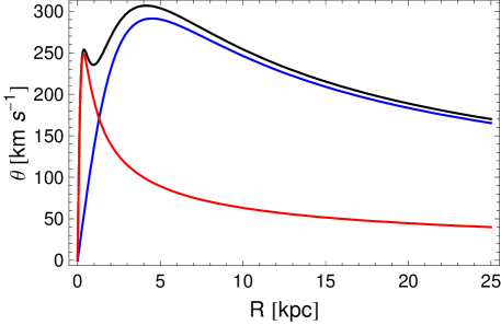
One important physical quantity in disk galaxies is the circular velocity in the plane ,
| (3) |
Replacing with our potential we obtain
| (4) |
A plot of for our galactic model with and is presented in Fig. 1, as a black curve. In the same plot, the red line shows the contribution from the spherical nucleus, while the blue curve is the contribution from the disk. It is seen that at small distances from the galactic center, kpc, the contribution from the spherical nucleus dominates, while at larger distances, kpc, the disk contribution is the dominant factor. We also observe the characteristic local minimum of the rotation curve which appears when fitting observed data to a Galactic model (e.g., Irrgang et al., 2013; Gómez et al., 2010).
Since the total potential is axisymmetric, the -component of the angular momentum is conserved. With this restriction, orbits can be described by means of the effective potential (e.g., Binney & Tremaine, 2008)
| (5) |
The term represents a centrifugal barrier; only orbits with small are allowed to pass near the axis of symmetry. The 3D motion is thus effectively reduced to a 2D motion in the meridional plane , which rotates non-uniformly around the axis of symmetry according to
| (6) |
where the dot indicates derivative with respect to time. The equations of motion on the meridional plane are
| (7) |
The equations governing the evolution of a deviation vector which joins the corresponding phase space points of two initially nearby orbits, needed for the calculation of the standard indicators of chaos, are given by the variational equations
| (8) |
The corresponding Hamiltonian to the effective potential given in Eq. (5) can be written as
| (9) |
where is the numerical value of the Hamiltonian, which is conserved. Therefore, an orbit is restricted to the area in the meridional plane satisfying .
3 Computational methods
In order to study the chaoticity of our models, we chose, for each set of values of the parameters of the potential, a grid of initial conditions in the plane, regularly distributed in the area allowed by the value of the energy. The points of the grid were separated 0.1 units in and 0.5 units in . For each initial condition, we integrated the equations of motion (7) with a double precision Bulirsch-Stoer algorithm (e.g., Press et al., 1992). Each orbit was integrated for time units, which corresponds to a time span of the order of hundreds of orbital periods. In all cases, the energy integral (Eq. (9)) was conserved better than one part in , although for most orbits it was better than one part in .
For our study, we want to know whether each orbit is regular or chaotic. Several indicators of chaos are available in the literature; we chose two of them, namely the standard Lyapunov exponents (e.g. Jackson, 1991) and the SALI indicator (Skokos et al., 2004). Of course, being the Lyapunov exponents defined for , only a finite time version of them (Lyapunov characteristic numbers) are numerically achievable. To compute these indicators, we integrated, along with each orbit, its corresponding variational equations (8) from unitary displacements in each of the Cartesian directions of the phase space of the meridional plane, thus allowing us to compute, along with the SALI, the full set of Lyapunov exponents using a Gram-Schmidt orthogonalization and a renormalization of the displacement vectors at each step, following the recipe of Bennetin et al. (1980).
To classify an orbit as regular or chaotic by using either the maximal Lyapunov characteristic number (MLCN) or the SALI, a threshold value should be established separating both types of orbit. This is a delicate issue, as these thresholds are generally obtained by some statistical procedure or, even, by eye inspection of plots of the indicators versus time. Besides, whereas the results of different chaos indicators agree in general, there are also “sticky” orbits (i.e., chaotic orbits that behave as regular ones during long periods of time), that may be misclassified by one or another method depending of the threshold value used.
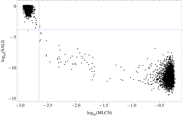
We established the thresholds by taking advantage of our computation of two chaos indicators, as follows. First, the set of orbits of a given grid was integrated, as we already said, for time units (i.e., about years, thus avoiding sticky orbits with a stickiness at least of the order of a Hubble time). Then, their MLCN and SALI were computed, and we looked for those values of the thresholds that maximised the agreement in the classification of both methods. To this end, we iterated the values of the thresholds until a minimum of disagreement has been achieved, choosing as initial values the mean of each indicator. We found that the values thus computed leave less than 1% of orbits differently classified by both methods. Fig. 2 shows an example of the resulting thresholds. The horizontal and vertical lines correspond to the established threshold values. We can see three red dots, corresponding to orbits for which the classifications of both indicators did not coincide. It is worth noticing that Kalapotharakos & Voglis (2005) also used a combination of MLCN and SALI, although they supplemented those indicators by adding the computation of the variation with time of the fundamental frequencies of the orbits, and they did not combine the indicators to establish their thresholds. As a reference, Table 1 shows the values of the thresholds thus obtained for each of the models studied in Section 4, plus the number of orbits which didn’t get the same classification.
| 0-500 | 0.25 | 10 | 74050 | 11 | |||
|---|---|---|---|---|---|---|---|
| 100 | 0.05-0.50 | 10 | 64092 | 11 | |||
| 400 | 0.25 | 1-50 | 71425 | 13 | |||
| 50 | 0.25 | 10 | 8993 | 1 | |||
| 50 | 0.25 | 10 | 8223 | 1 | |||
| 50 | 0.25 | 10 | 7429 | 2 | |||
| 50 | 0.25 | 10 | 6575 | 2 | |||
| 50 | 0.25 | 10 | 5665 | 2 | |||
| 50 | 0.25 | 10 | 4685 | 2 | |||
| 50 | 0.25 | 10 | 3613 | 0 | |||
| 50 | 0.25 | 10 | 2473 | 0 | |||
| 50 | 0.25 | 10 | 1309 | 0 | |||
| 50 | 0.25 | 10 | 255 | 0 | |||
| 100 | 0.15 | 10 | 9079 | 0 | |||
| 100 | 0.15 | 10 | 8314 | 0 | |||
| 100 | 0.15 | 10 | 7506 | 0 | |||
| 100 | 0.15 | 10 | 6644 | 0 | |||
| 100 | 0.15 | 10 | 5742 | 0 | |||
| 100 | 0.15 | 10 | 4758 | 0 | |||
| 100 | 0.15 | 10 | 3703 | 0 | |||
| 100 | 0.15 | 10 | 2550 | 0 | |||
| 100 | 0.15 | 10 | 1362 | 0 | |||
| 100 | 0.15 | 10 | 320 | 0 | |||
| 500 | 0.25 | 10 | 9592 | 1 | |||
| 500 | 0.25 | 10 | 8812 | 2 | |||
| 500 | 0.25 | 10 | 7991 | 2 | |||
| 500 | 0.25 | 10 | 7111 | 0 | |||
| 500 | 0.25 | 10 | 6189 | 0 | |||
| 500 | 0.25 | 10 | 5188 | 0 | |||
| 500 | 0.25 | 10 | 4111 | 0 | |||
| 500 | 0.25 | 10 | 2960 | 0 | |||
| 500 | 0.25 | 10 | 1755 | 0 | |||
| 500 | 0.25 | 10 | 642 | 0 |
Once the orbits have been classified into chaotic or non-chaotic, we considered those of this last set as regular orbits.222A regular orbit of a -dimensional potential obeys, by definition, or more isolating integrals of motion. On the other hand, a chaotic orbit is defined through its sensitivity to the initial conditions in phase space: if the initial conditions of the orbit are infinitesimally displaced, then the distance between the original orbit and the new orbit grows exponentially with time. These definitions do not complement each other. Whereas it can be proved that a regular orbit is not chaotic and a chaotic orbit is not regular (e.g., Jackson, 1991, Section 8.3), as far as we know it has not been proved that every irregular (i.e. not regular) orbit is chaotic, or, in other words, that every orbit obeying less than isolating integrals has sensitivity to the initial conditions. Nevertheless, to avoid confusion, we will follow here the widespread convention of considering irregular orbits and chaotic orbits as the same set. We then further classified these regular orbits into families, by using the frequency analysis of Carpintero & Aguilar (1998), although the extraction of frequencies was done with the frequency modified Fourier transform, an algorithm first developed by Laskar (1988) and later improved by Šidlichovský and Nesvorný (1996).
A note about the nomenclature of orbits. All the orbits of an axisymmetric potential are 3D loop orbits, i.e., orbits that rotate around the axis of symmetry always in the same direction. However, in dealing with the meridional plane the rotational motion is lost, so the path that the orbit follows onto this plane can take any shape, depending on the nature of the orbit. We will call an orbit according to its behaviour in the meridional plane. Thus, if for example an orbit is a rosette lying in the equatorial plane of the axisymmetric potential, it will be a linear orbit in the meridional plane, etc.
4 Results
In this Section, we will complement our indicators of chaos, MLCN and SALI, with the classical method of the Poincaré Surface of Section (PSS), in order to visually distinguish the regular or chaotic nature of motion. We used the initial conditions mentioned in Sec. 3 in order to build the respective PSSs, taking values inside the Zero Velocity Curve (ZVC) defined by
| (10) |
Since we want to investigate how the parameters of the dynamical system influence not only the level of chaos but also the percentages of the basic families of regular orbits, we chose to study the following seven basic families: (a) box orbits, (b) 1:1 linear orbits, (c) 2:1 banana-type orbits, (d) 2:3 fish-type orbits, (e) 4:3 resonant orbits, (f) 4:5 resonant orbits and (g) orbits with higher resonances, i.e., all resonant orbits not included in the former categories. It turns out that for these last orbits the corresponding percentage is less than 1% in all cases, and therefore their contribution to the overall orbital structure of the galaxy is insignificant. Note that every resonance is expressed in such a way that is equal to the total number of islands of invariant curves produced in the phase plane by the corresponding orbit. In Fig. 3 we present an example of each of the seven basic types of regular orbits, plus an example of a chaotic one. In all cases, we set (except for the chaotic orbit, where ), , , . The orbits shown in Figs. 3a and 3h were computed until time units, while the rest were computed until one period has completed. The curve circumscribing each orbit is the limiting curve in the plane defined as . Table 2 shows the initial conditions for each of the depicted orbits; for the resonant cases, the initial conditions and the period correspond to the parent periodic orbit.

| Orbit | Figure | |||
|---|---|---|---|---|
| box | 3a | 7.41800000 | 0.000000000 | - |
| 2:1 banana | 3b | 4.40634102 | 0.000000000 | 1.22699769 |
| 1:1 linear | 3c | 3.36734581 | 31.97732133 | 0.95200932 |
| 2:3 fish | 3d | 9.61363706 | 0.000000000 | 1.93809874 |
| 4:3 boxlet | 3e | 7.78008196 | 0.000000000 | 3.67094043 |
| 4:5 boxlet | 3f | 9.27613711 | 0.000000000 | 3.85375364 |
| 6:5 boxlet | 3g | 8.30441195 | 0.000000000 | 5.60252420 |
| chaotic | 3h | 10.72000000 | 0.000000000 | - |
It is worth noticing that the 1:1 resonance is usually the hallmark of loop orbits, both coordinates oscillating with the same frequency in their main motion. Their mother orbit is a closed loop orbit. Moreover, when the oscillations are in phase, the 1:1 orbit degenerates into a linear orbit (the same as in Lissajous figures made with two oscillators). In our meridional plane, however, 1:1 orbits do not have the shape of a loop. Their mother orbit is linear (as in Fig. 3c), and thus they don’t have a hollow (in the meridional plane) but fill a region around the linear mother, always oscillating in and with the same frequency. We will call them “1:1 linear open orbits” to differentiate them from true meridional plane loop orbits, which have a hollow and rotate always in the same sense.
4.1 Influence of the mass of the nucleus
To study how the mass of the nucleus influences the level of chaos, we let it vary while fixing all the other parameters of our model. As already said, we fixed the values , and . We chose as a fiducial value for the size of the nucleus, and integrate orbits in the meridional plane for the set . In all cases the energy was set to and the angular momentum of the orbits . Once the values of the parameters were chosen, we computed a set of initial conditions as described in Sec. 3, and integrated the corresponding orbits computing at the same time the two chaos indicators. The respective thresholds and resulting classifications were computed once the entire set was fully integrated.
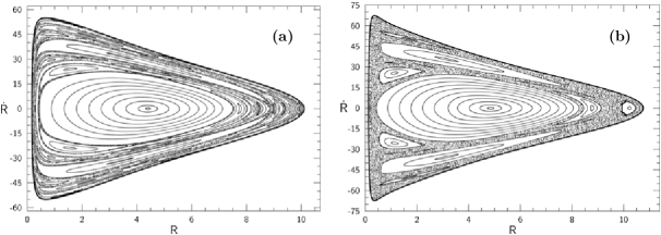
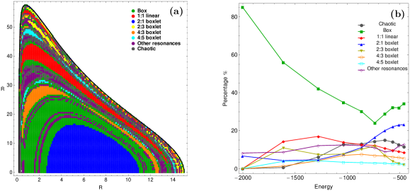
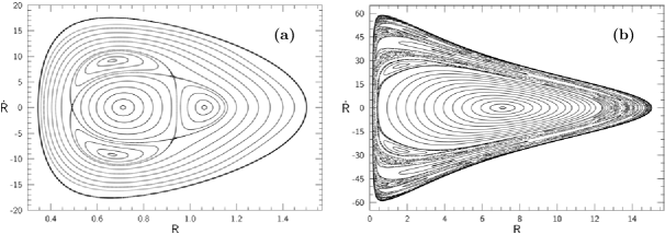
Fig. 4a depicts the phase plane when . One can observe that most of the phase space is covered by regular orbits, while there are also several chaotic layers which separate the areas of regularity. Thus, there is not a unified chaotic domain, at least in this slice of the phase space. The outermost thick curve is the ZVC. In Fig. 4b we present the phase plane when , i.e., a model with a more massive nucleus. It is evident that there are many differences with respect to Fig. 4a, being the most visible the growth of the region occupied by chaotic orbits, the presence of a large unified chaotic sea, and an increasing in the allowed radial velocity of the stars near the center of the galaxy.
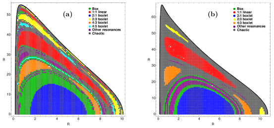
Figs. 5a and 5b show grids of orbits that we have classified on the PSS of Figs. 4a and 4b, respectively. Here we can see which of the regular families each of the islands seen in the PSSs belong to. In Fig. 5a appear the seven main families already mentioned: (i) 2:1 banana-type orbits correspond to the invariant curves surrounding the central periodic point in the corresponding PSS; (ii) box orbits are situated mainly outside of the 2:1 resonant orbits; (iii) 1:1 open linear orbits form the double set of elongated islands in the PSS; (iv) 2:3 fish-type orbits form the outer triple set of islands of the PSS; (v) 4:3 resonant orbits correspond to the middle triple set of islands in the PSS; (vi) 4:5 resonant orbits form the chain of five islands of the PSS; and (vii) there are many other types of resonances producing several chains of small islands in the PSS, embedded in the chaotic layers. The white dots inside the grid correspond to orbits that have been classified as regular by one of the indicators and chaotic by the other, being most probably sticky orbits. The outermost black thick curve is the ZVC. On the other hand, in Fig. 5b the basic families of orbits are still present except for the 4:5 family which has disappeared making room for chaotic orbits. Also, the portion of higher resonant orbits is considerably smaller than in Fig. 5a.
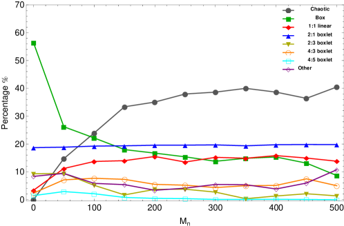
Fig. 6 shows the resulting percentages of chaotic orbits and of the mean families of regular orbits as varies. It can be seen that when the nucleus is absent, there is no chaos whatsoever, and most orbits are box orbits. However, a small nucleus is enough to trigger chaotic phenomena, whereas the box orbits are depleted. This trend continues, although at a lesser rate, as the nucleus grows in mass, i.e., the percentage of box orbits is reduced and that of chaotic orbits is increased. The rest of orbits change very little; the meridional bananas, in fact, are almost unperturbed by the shifting of the mass of the nucleus. From this figure, one may conclude that affects mostly the box and chaotic orbits in our galactic model.
4.2 Influence of the scale length of the nucleus
Now we proceed to investigate how the scale length of the nucleus influences the amount of chaos. Again, we let it vary while fixing all the other parameters of our galactic model, choosing as a fiducial value for the mass of the nucleus, and integrating orbits in the meridional plane for the set . As before, the energy was set to and .
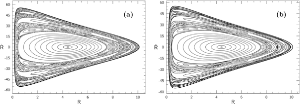
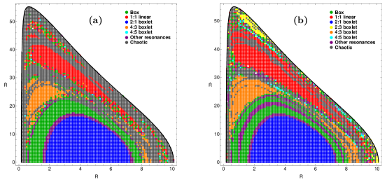
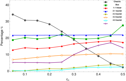
Fig. 7a presents the phase plane when . We observe that much of it is covered by islands of regular orbits, surrounded by a chaotic sea. Fig. 7b corresponds to the case, i.e., a less concentrated spherical nucleus. As can be seen, there are no big differences between both cases, the most prominent one being the shrinking of the area occupied by chaotic orbits. In fact, the chaotic sea has been separated into different regions which surround all the sets of invariant curves produced by the regular orbits. Fig. 8a, made as Fig. 5a but for the PSS of Fig. 7a, shows that there are present only six out of the seven main families of regular orbits: the 2:3 resonance is absent, while the islands of the 4:5 resonant orbits are so thin that they appear as lonely points in the grid. On the other hand, in Fig. 8b, corresponding to , all the basic families of regular orbits are present. Also, the region of orbits of high resonances is considerably larger than with . This trend is fairly visible in Fig. 9, where the resulting percentages of chaotic and regular orbits as varies are shown. It can be seen that there is a strong correlation between the percentage of chaotic orbits and the value of . At the same time, as the nucleus become less concentrated, there is a gradual increase in the percentage of almost all of the regular families, most noticeably the box and the high resonant boxlets. Once again, the meridional 2:1 bananas are immune to changes of the parameter. Thus, decreasing the scale length of the nucleus turns box and high resonant orbits into chaotic orbits, while those with low resonances are less affected.
4.3 Influence of the angular momentum
Zotos (2012b) showed, for an axially symmetric galactic model composed of a disk, a halo and a spherical nucleus, that one of the most important parameters that influences the orbital structure is the angular momentum . Here, we let vary along the set , while fixing , and . Fig. 10a depicts the phase plane when . We observe the existence of a large chaotic sea, while most of the regular orbits are located near the central region of the phase plane, although there are important islands of invariant curves surrounding them. In Fig. 10b, corresponding to , we can see that the amount of chaos is smaller, and that an additional inner chaotic layer has appeared besides the outer sea. In Fig. 10c we can see the phase plane when . It is seen that almost all the phase plane is covered by regular orbits. Nevertheless, we can still distinguish the presence of two distinct chaotic layers. In Fig. 10d, which shows the case , the entire phase plane is seen covered by regular orbits; the chaotic motion is negligible. From these figures we can draw two conclusions: (i) increasing causes a decreasing of the chaotic region, which eventually disappears almost completely and (ii) the permissible area on the phase plane is reduced as we increase the value of . Figs. 11(a-d) show the grids of orbits that we have classified, corresponding to the PSSs of Figs. 10(a-d) respectively. In Fig. 11a we note a lack of 4:5 boxlets orbits; they appear in Fig. 11b, although forming very thin islands. In Fig. 11c we observe a drastic decrease of chaotic orbits, thus leaving room to regular families. Fig. 11d shows that the regular orbits have taken almost all the phase plane. It is worth noticing that, at the highest angular momentum, the 4:3 resonance has been almost deleted from the phase plane.
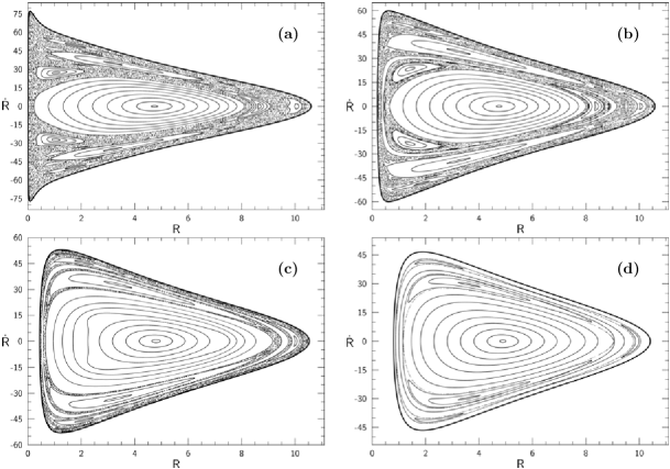
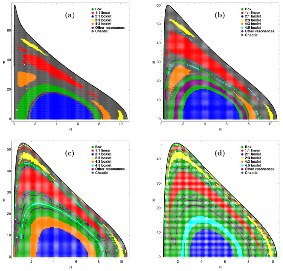
Fig. 12a presents the resulting percentages of chaotic and regular orbits as varies. It is clearly seen that, as increases, the percentage of chaotic orbits decreases almost linearly, while that of box orbits grows steadily when . In fact, when , they are the dominant type of orbits. The rest of orbits change less. In particular, the percentage of 2:1 bananas is little affected by the increase of the angular momentum, unlike the previous cases. It is also seen that when the percentage of the 4:3 family drops suddenly, remaining at very low values from then on. Summarizing, the angular momentum mostly affects box and chaotic orbits.
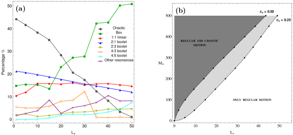
To further investigate the influence of , we define, for each set of values of the parameters, the critical value of the angular momentum as the maximum value of the angular momentum for which the orbits can display chaotic motion. Fig. 12b shows the numerically found relationship between and , for two values of the scale length of the nucleus, and . To obtain this, orbits were started near , with , and obtained from the energy integral with . Here, is the minimal root of the equation
| (11) |
The particular value of the energy was chosen so that in all cases kpc. It is seen in Fig. 12b that the relationship between and is nearly linear. This line divides the plane in two parts; orbits on the upper shaded part of the plot may be either regular or chaotic, while those on the lower part of the plot can only be regular. Moreover, it is interesting to notice that the extent of the chaotic domain is larger when the value of is smaller, that is, when the nucleus is more concentrated, which is in agreement with the results found in Fig. 9.
4.4 Influence of the energy
Another parameter that plays an important role is the value of the orbital energy . We investigated three cases: (i) A system with a small amount of chaos; for this case, we set , and . (ii) A system with a medium level of chaos, for which we chose , and . (iii) A system which presents a large amount of chaos, with , and . To select the energy levels, we chose for each case the ten energies which give , where is the maximum possible value of on the phase plane.
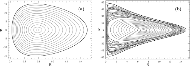
For the case (i), low level of chaos, Fig. 13a depicts the phase plane when which corresponds to . It is seen that the entire phase space is covered by regular orbits. In Fig. 13b we present the phase plane when (). Here, the chaotic orbits have taken a small region of the phase plane, which is nevertheless still mainly occupied by regular families. Fig. 14a shows a grid of orbits that we have classified on the PSS of Fig. 13b. We can see that all the different types of orbits are present, although most of them correspond to either box orbits or 2:1 banana-type orbits. Also, the 1:1 and 4:3 resonances occupy a significant portion of the PSS, while the 2:3 and the 4:5 resonances appear to be confined in small islands. Fig. 14b shows the resulting percentages of chaotic and regular orbits as varies. It can be seen that when the motion of stars is at very low energies, it is entirely regular, being the box orbits the all-dominant type. The percentage of box orbits is however reduced as the energy is increased, although they always remain the most populated family. It is also seen that the percentages of 1:1 and 2:3 boxlets start to grow as soon as the energy grows, but then they remain at relatively low values, the 2:3 family disappearing at high energies. The percentage of orbits of the 2:1 family, on the other hand, takes relatively high values at high energies. Only the 4:5 boxlet orbits remain almost unperturbed by the increase of the energy. These percentages show that, when there is a small amount of chaos, the value of the energy affects mostly the regular orbits by shifting the population of the different families.
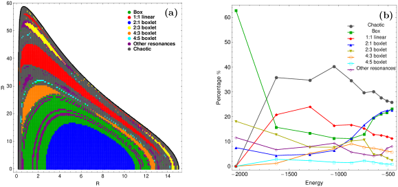
For the case (ii), Fig. 15a depicts the phase plane when which corresponds to . Once again, the phase plane is almost entirely covered by regular orbits, while the chaotic motion is negligible. In Fig. 15b we present the phase plane when and , where a chaotic outer area is clearly seen, and an additional inner thin chaotic layer can be observed. Fig. 16a shows a grid of orbits that we have classified on the PSS of Fig. 15b. It is seen that the majority of orbits correspond either to chaotic, box, or 2:1 banana-type orbits. The 1:1, 2:3 and 4:3 resonances occupy a significant portion of the PSS forming well-defined islands. It is also worth mentioning that there is a considerable amount of higher resonant orbits. Fig. 16b presents the resulting percentages of the different orbits as varies. Once again, low energy orbits, i.e., orbits which move near the center, are almost entirely box orbits (in the meridional plane). Also, the 2:1 bananas start to grow in percentage at high energies. But, unlike case (i), the percentage of box orbits is significantly reduced as grows, and, at the same time, the chaotic and the 1:1 orbits increase rapidly. The level of chaoticity remains relatively high, around 30-40%. At the higher energy studied in case (ii), the percentages of the chaotic, box and 2:1 orbits tend to a common value (around 25%), sharing three fourths of the entire phase plane.
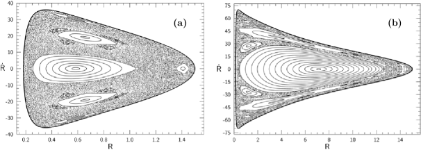
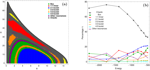
With respect to case (iii), high level of chaos, Fig. 17a shows the phase plane when which corresponds to . It is seen that most of the phase plane is covered by chaotic orbits. In Fig. 17b we present the phase plane when and . Here, we have a significant decrease in the region occupied by chaotic orbits. Fig. 18a shows the grid of orbits corresponding to the PSS of Fig. 17b. We see that most orbits are chaotic, although all the regular families, with the exception of the 4:5 family, occupy a significant portion of the PSS. In Fig. 18b, which presents the resulting percentages, it can be seen that the motion is highly chaotic throughout. Though the percentage of chaotic orbits is gradually reduced as the energy increases, it remains larger than any other individual regular family. From on, the decreasing of chaotic orbits is paired with a similar increasing of box and 2:1 orbits. As before, the 4:5 orbits remain unperturbed and with very low percentages
5 Analysis of the results
In the literature, the dynamical origin of the onset of chaos has proven elusive so far. A promising line of investigation, namely the curvature of the phase space, although theoretically sound, came up against many experimental counterexamples (e.g., Szydlowski, 1994). So, we will not attempt to explain which dynamical factors are responsible for the onset and growth of chaos, but try to isolate any behaviour that may be correlated with that.
Gerhard & Binney (1985) have shown that stars that pass near a density cusp, thus receiving a large acceleration, may depopulate the family of box orbits which supports the triaxial figure of a galaxy. Therefore, regions of large accelerations may be responsible for the onset of chaos. Since our potential is nowhere divergent, we do not have any cusps. But, the effective potential on the meridional plane does have a cusp at the origin, caused by the centrifugal term. Thus, we seek whether there is a relationship between chaos and a star going near the origin.
We computed, for each star of our models, their minimum distance (in the meridional plane) to the origin of coordinates. Fig 19a shows these minimum distances for all the orbits used to study the influence of the mass of the bulge , versus the value of their respective MLCNs; the horizontal line indicates the threshold between regular and chaotic orbits. It is seen that all the chaotic orbits pass near the center, i.e., they suffer at one time or another some sudden acceleration due to the centrifugal force. On the other hand, we can see that this is not a sufficient condition to be chaotic: regular orbits can also pass near the center. We’ve found exactly the same behaviour when using orbits from the rest of the cases analysed in Section 4. Therefore, we may draw the following conclusion: in the meridional plane of our galactic model, a necessary condition for an orbit to be chaotic is to pass near the center of the potential; a sufficient condition for an orbit to be regular is not to pass near the center of the potential.

From the results of the previous Section, all of the studied parameters, except the energy, have an almost monotonic influence on the percentage of chaos in the meridional plane. This percentage grows with the increment of the mass of the bulge (Fig. 6), the decrement of the scale length of it (Fig. 9), and the decrement of the angular momentum (Fig. 12, left). We’ve found (numerically) that in all the cases the position of the minimum of the effective potential, which is always located on the axis (e.g., Binney & Tremaine, 2008), nears the origin of coordinates whenever the percentage of chaos rises. Fig. 19b shows the minimum distance to the origin for the orbits shown in Fig 19a, versus their minimum distances to . We can see a consistent correlation between those quantities, hinting that the position of the minimum of the effective potential might influence the degree of chaos, although we weren’t be able to find an analytic proof of this.
The picture described above is consistent with the rising of the percentage of the chaotic motion with (Fig. 6), since the acceleration grows with the mass of the bulge (Sec. 2). Also, it is consistent with the behaviour of the chaotic percentage seen in Fig. 9, considering that the more concentrated is the nucleus, the more acceleration it causes near the center. It also explains why the percentage of chaotic motion diminishes when the angular momentum increases (Fig. 12a), given that a low angular momentum allows the star to approach the center of the potential. On the other hand, Fig. 6 shows that when the bulge is absent, there is no chaotic motion at all. Whereas this proves that the onset of chaos is driven by the presence of the nucleus, it also poses a question mark about the abovementioned role of the centrifugal force, since it is at work even in this full regular case.
On the other hand, as it was seen in the previous Section, the variation of the parameters , , and causes not only variations in the chaotic content, but also in the relative importance of the different regular families. In particular, the 4:5 resonance may be taken as a model, since it appears mainly when there is a low level of chaos, and decreases significantly or even disappears when we have a strong chaotic regime. Therefore, it is of particular interest to investigate how its stability is being influenced by the above-mentioned parameters. For this purpose, we used the theory of periodic orbits (Meyer & Hall, 1992), in which the stability criteria can be obtained from the elements of the monodromy matrix as follows:
| (12) |
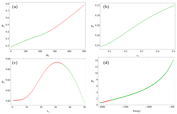
where Tr stands for the trace of the matrix, and is called the stability index. For each set of values of , , and , we first located, by means of an iterative process, the position of the parent 4:5 orbit onto the axis when . Then, using these initial conditions plus the value of obtained from the energy, we integrated the variational equations in order to obtain the matrix , with which we computed the index . The results are presented in Figs. 20 (a-d). In Fig. 20a we can see the evolution of the position and of the stability of the 4:5 resonance when varies, the values of all the other parameters being as in Fig. 6. Green dots correspond to stable periodic orbits, while red dots correspond to unstable ones. We can see that when the periodic orbit becomes unstable. Curiously, it is also unstable when . On the other hand, in Fig. 20b we see that the stability of the 4:5 parent periodic orbit is completely unaffected by the scale length of the nucleus. In this case, the values of all the other parameters are as in Fig. 9. In Fig. 20c, where we have used the values of the parameters as in Fig. 12 (left), it can been seen that there is a limit of stability around . It is worth noticing that, though in Fig. 11a there is no evidence of a 4:5 resonance, Fig. 20c indicates that the resonance is indeed present, although evidently deeply buried in the chaotic sea. Finally in Fig. 20d we present the influence of the value of the energy. The values of all the other parameters are as in Fig. 16 (right). One may see that most of the periodic orbits are stable, except the region in which the periodic orbits become unstable. It is clear, then, that the parameters of the model, as well as the isolating integrals of motion, play a fundamental role in the stability of the regular families, which in turn determines which ones are present in each case.
6 Discussion and Conclusions
We have investigated how influential are the parameters of a disc galaxy with bulge on the level of chaos and on the distribution of regular families among its orbits. We have used an analytic axisymmetric potential which embraces the general features of a disc galaxy with bulge, and have chosen to work in the meridional plane of the orbits, in order to simplify the study. Varying several of the constants of the potential, as well as the two global isolating integrals of the orbits, namely the angular momentum and the energy, we have found that the level of chaos and the distribution in regular families is indeed very dependent on all of these parameters.
Our study shows that the mass of the bulge, although spherically symmetric and therefore maintaining the axial symmetry of the whole galaxy, generates chaos in the meridional plane as soon as it is above zero. As the mass increases, this chaotic motion grows in percentage at the expense of the (meridional plane) box orbits, although it seems to saturate at % of the orbits once the mass of the bulge has reached some % of the mass of the disc. The concentration of the bulge plays a similar role: the percentage of chaotic motion depends almost linearly on this parameter. Once more, box orbits and high-resonance orbits (by which we mean resonant orbits with a rational quotient of frequencies made from integers ) are the ones that give way to the chaotic orbits. We also found that the angular momentum of the orbits influences the level of chaos in a similar fashion: orbits with low angular momenta have higher chances of being chaotic that those with high values of it. The relationship between chaos and angular momentum is close to linear, and, again, box orbits are the most affected by the percentage of chaos. The energy of the orbits, however, plays a different role. In a model with low level of chaos, varying the energy mainly shuffles the orbital content among the families of regular orbits. Interestingly, box orbits are again the family which suffers the most. Taking a model with a medium level of chaos, box orbits are the dominant family at low energies, but the percentage of chaos quickly grows as the energy increases, again by collapsing the percentage of box orbits. In this case, however, linear orbits (i.e., 3D hollowed out saucers) grow along with chaotic ones; also, further increasing the energy reverts these trends, and 2:1 bananas start to increase their share. With a high level of chaos model, the increase of the energy diminishes the percentage of chaos, while the box and 2:1 bananas take the field.
When taken into account that the effective potential in the meridional plane has a cusp caused by the centrifugal acceleration, all these behaviours turn out to be consistent with the analysis we made on Sec. 5, where we arrived to the conclusion that a necessary condition for an orbit to be chaotic is to pass near the center of the potential, and a sufficient condition for an orbit to be regular is not to pass near the center of the potential.
In the same vein, we also conducted an investigation on the stability of the 4:5 resonance, which was taken as a model, in an attempt to see whether it depends on the parameters of the galactic system and the integrals of motion. Our results indicate that, with the exception of the scale length of the nucleus, all the parameters affect substantially the stability of this family, hinting at a deep interplay between chaos and proportion of regular families.
We’ve also found that, by combining the MLCN and the SALI algorithms, we can obtain for both methods reliable thresholds separating chaotic from regular motion.
We consider the outcomes of the present research as an initial effort in the task of exploring the orbital structure of a disk galaxy with a central spherical nucleus. Since our results are encouraging, it is in our future plans to study the influence of all the available parameters, including the disk’s parameters , and . Moreover, we plan to obtain the entire network of periodic orbits and reveal the evolution of their stability with respect to all the parameters of the galactic model.
Acknowledgments
The authors would like to thank the anonymous referee for the careful reading of the manuscript and for all the aptly suggestions and comments which allowed us to improve both the quality and the clarity of our work. This work was supported with grants from the Universidad Nacional de La Plata (Argentina), the Consejo Nacional de Investigaciones Científicas y Técnicas de la República Argentina, and the Agencia Nacional de Promoción Científica y Tecnológica (Argentina).
References
- Allen & Santillán (1991) Allen, C., Santillán, A.: An improved model of the galactic mass distribution for orbit computations. Rev. Mex. Astron. Astrof. 22, 255-263 (1991)
- Bennetin et al. (1980) Bennetin, G., Galgani, G., Giorgilli, A., Strelcyn, J. M.: Lyapunov characteristic exponents for smooth dynamical systems and for Hamiltonian systems; a method for computing all of them. Part 1: theory; Part 2: numerical applications. Meccanica 15, 9-20, 21-30 (1980)
- Binney & Spergel (1982) Binney, J., Spergel, D.: Spectral stellar dynamics. ApJ 252, 308-321 (1982)
- Binney & Spergel (1984) Binney, J., Spergel, D.: Spectral stellar dynamics. II - The action integrals. MNRAS 206, 159-177 (1984)
- Binney & Tremaine (2008) Binney, J., Tremaine, S.: Galactic Dynamics, Princeton Univ. Press, Princeton, USA (2008)
- Caranicolas & Vozikis (1986) Caranicolas, N., Vozikis, Ch.: Orbital characteristics of dynamical models of elliptical galaxies. Cel. Mech. 39, 85-102 (1986)
- Carpintero & Aguilar (1998) Carpintero, D.D., Aguilar, L.A.: Orbit classification in arbitrary 2D and 3D potentials. MNRAS 298, 1-21 (1998)
- Contopoulos (1960) Contopoulos, G.: A third integral of motion in a galaxy. Z. Astroph. 49, 273-291 (1960)
- Contopoulos (1979) Contopoulos, G.: in Stochastic behavior in classical and quantum Hamiltonian systems, G. Casati and J. Ford Eds., p. 1–17. DOI: 10.1007/BFb0021732 (1979)
- Copin et al. (2000) Copin, Y., Zhao, H., de Zeeuw, P.: Probing a regular orbit with spectral dynamics. MNRAS 318, 781-797 (2000)
- Gerhard & Binney (1985) Gerhard, O., Binney, J.: Triaxial galaxies containing massive black holes or central density cusps. MNRAS 216, 467-502 (1985)
- Gerhard & Saha (1991) Gerhard, O., Saha, P.: Recovering galactic orbits by perturbation theory. MNRAS 251, 449-467 (1991)
- Gómez et al. (2010) Gómez, F., Helmi, A., Brown, A.G.A., Li, Y.-S.: On the identification of merger debris in the Gaia era. MNRAS 408, 935-946 (2010)
- Greiner (1987) Greiner, J.: A new kind of stellar orbit in a galactic potential. Cel. Mech. 40, 171-175 (1987)
- Greiner (1991) Greiner, J.: Higher order resonant orbits. Cel. Mech. and Dyn. Ast. 50, 387-394 (1991)
- Hasan & Norman (1990) Hasan, H., Norman, C.A.: Chaotic orbits in barred galaxies with central mass concentrations. ApJ 361, 69-77 (1990)
- Hasan et al. (1993) Hasan, H., Pfenniger, D., Norman, C.: Galactic bars with central mass concentrations - Three-dimensional dynamics. ApJ 409, 91-109 (1993)
- Irrgang et al. (2013) Irrgang, A., Wilcox, B., Tucker, E., Schiefelbein, L.: Milky Way mass models for orbit calculations. A&A 549, A137 (2013)
- Jackson (1991) Jackson E.A.: Perspectives of nonlinear dynamics, Cambridge Univ. Press, Cambridge (1991)
- Kalapotharakos & Voglis (2005) Kalapotharakos, C., Voglis, N.: Global Dynamics in Self-Consistent Models of Elliptical Galaxies. Cel. Mech. & Dyn. Astr. 92, 157-188 (2005)
- Karanis & Caranicolas (2001) Karanis, G.I., Caranicolas, N.D.: Transition from regular motion to chaos in a logarithmic potential. A&A 367, 443-448 (2001)
- Laskar (1988) Laskar, J.: Secular evolution of the solar system over 10 million years. A&A 198, 341-362 (1988)
- Laskar (1993) Laskar, J.: Frequency analysis for multi-dimensional systems. Global dynamics and diffusion. Physica D 67, 257-281 (1993)
- Lees & Schwarzschild (1992) Lees, J.F., Schwarzschild, M.: The orbital structure of galactic halos. ApJ 384, 491-501 (1992)
- Manabe (1979) Manabe, S.: Applicability of Approximate Third Integral of Motion for Stellar Orbits in the Galaxy. Pub. Ast. Soc. Japan 31, 369-394 (1979)
- Manos & Athanassoula (2011) Manos, T., Athanassoula, E.: Regular and chaotic orbits in barred galaxies - I. Applying the SALI/GALI method to explore their distribution in several models. MNRAS 415, 629-642 (2011)
- Manos et al. (2008) Manos, T., Skokos, Ch., Athanassoula, E., Bountis, T.: Studying the global dynamics of conservative dynamical systems using the SALI chaos detection method. Nonlin. Phenom. Complex Syst. 11, 171-176 (2008)
- Martinet & Mayer (1975) Martinet, L., Mayer, F.: Galactic orbits and integrals of motion for stars of old galactic populations. III - Conclusions and applications. A&A 44, 45-57 (1975)
- Meyer & Hall (1992) Meyer, K.R., Hall, G.R.: Introduction to Hamiltonian Dynamical Systems and the N-Body Problem. Springer-Verlag (1992)
- Miyamoto & Nagai (1975) Miyamoto, M., Nagai, R.: Three-dimensional models for the distribution of mass in galaxies. Publ. Astron. Soc. Jpn. 27, 533-543 (1975)
- Ollongren (1965) Ollongren, A.: Theory of stellar orbits in the galaxy. Ann. Rev. A&A 3, 113-134 (1965)
- Ollongren (1966) Ollongren, A.: Construction of galactic stellar orbits similar to harmonic oscillators. AJ 72, 436-442 (1967)
- Press et al. (1992) Press, H.P., Teukolsky, S.A, Vetterling, W.T., Flannery, B.P.: Numerical Recipes in FORTRAN 77, 2nd Ed., Cambridge Univ. Press, Cambridge, USA (1992)
- Šidlichovský and Nesvorný (1996) Šidlichovský, M., Nesvorný, D.: Frequency modified Fourier transform and its applications to asteroids. Cel. Mech. & Dyn. Ast. 65, 137-148 (1996)
- Skokos et al. (2004) Skokos, Ch., Antonopoulos, Ch., Bountis, T.C., Vrahatis, M.N.: Detecting order and chaos in Hamiltonian systems by the SALI method. J. Phys. A: Math. Gen. 37, 6269-6284 (2004)
- Szydlowski (1994) Szydlowski, M.: Curvature of gravitationally bound mechanical systems. J. Math. Phys. 35, 1850-1880 (1994)
- Wilkins (1989) Wilkins, G.A.: The IAU Style Manual, in IAU Transactions XXB, p. S23 (1989)
- Zotos (2012a) Zotos, E.E.: Trapped and escaping orbits in an axially symmetric galactic-type potential. PASA 29, 161-173 (2012)
- Zotos (2012b) Zotos, E.E.: Exploring the nature of orbits in a galactic model with a massive nucleus. New Astron. 17, 576-588 (2012)