Statistical pairing fluctuation and phase transition in ${}^{94}Mo$

Abstract

In the framework of BCS model, we have applied the isothermal probability distribution to take into account the statistical fluctuations in calculation of thermodynamical properties of nuclei. The energy and the heat capacity are calculated in ${}^{94}Mo$ nucleus using the mean gap parameter. The results are compared with the values obtained based on the most probable values, experimental data as well as some other theoretical models. We have shown that heat capacity versus temperature behaves smoothly instead of singular behavior predicted by the standard BCS model. Also a smooth peak in heat capacity is observed which is a signature of transition from normal to superfluid phase.
PACS numbers: 21.10.-k, 21.60.-n

I Introduction

Recently a lot of effort has been paid to describe the behavior of paired small systems, such as metallic clusters and nuclei. The starting point in all these methods is pairing hamiltonian of the system under study. Various methods are used to calculate the partition(or grand partition) function and they are different in how the constraint of fixed number of particles is considered in the calculations. Some of the methods such as the Static-Path Approximation(SPA) plus Random-Phase Approximation(RPA) rr ; kk use number projected partition function. Some others as Lipkin-Nogami method hj ; yn ; hc add non-extensive terms to the free energy to fix the particle number. In the BCS method jb ; lg2 grand partition function is used to obtain thermodynamic functions of the system. The BCS uses the most probable value of pairing gap parameter which for few particle systems like nucleus leads to prediction of some unreal singularities in heat capacity that is due to of ignoring the impact of fluctuations in such systems. Experiments conducted by Oslo Group kke show a very smooth variation of heat capacity versus temperature, with a peak which is believed to be due to a phase transition in nuclei. To tackle the problem of singularities in BCS we must take into account the effect of fluctuations. So we have used the isothermal probability distribution ld ; lg , which states the probability of a system to be in a specific configuration is proportional to the exponential of it’s free energy. Using this principal we calculate the mean value of gap parameter and then the thermodynamic properties of nuclei based on of the mean value of pairing gap parameter instead of the most probable value.

II Model

The BCS is the standard theory to deal with a system of fermions having pairing potential. The main tool which is used to obtain thermodynamic properties in this method is the grand potential of the system, $\Omega$, which has the following form in the mean field approximation:

$$\Omega=-\beta\sum(\varepsilon_{k}-\lambda-E_{k})+2\sum\ln(1+\exp(-\beta E_{k}))-\beta\frac{\Delta^{2}}{G}$$ (1)

where $\varepsilon_{k}$ is single particle energy of particles,$E_{k}=\sqrt{(\varepsilon_{k}-\lambda)^{2}+\Delta^{2}}$ is quasi particle energy, $G$ is the pairing strength, $\lambda$ is the chemical potential and $\beta=\frac{1}{T}$, where $T$ is the temperature. In this equation $\Delta$ is the gap parameter which is a measure of the pairing correlation. Thermodynamic quantities of the system, such as the number of particles $N$, the energy of the system $E$ and the entropy $S$ are calculated from following relations.

$$N=\frac{\partial\Omega}{\partial\alpha}\ \ \ ,\ \ \ E=-\frac{\partial\Omega}{\partial\beta}\ \ \ ,\ \ \ S=\Omega-\alpha N+\beta E\ \ \ \ \ \ \ \ (\alpha=\beta\lambda)$$ (2)

The standard procedure to calculate gap parameter is minimizing the free energy

$$\frac{\partial\Omega}{\partial\Delta}=0$$ (3)

which leads to the BCS gap equation

$$\sum\frac{1}{E_{k}}\tanh(\frac{1}{2}\beta E_{k})=\frac{2}{G}.$$ (4)

Using this equation, the following relations for thermodynamic quantities will be obtained:

$$N=\sum[1-\frac{\varepsilon_{k}-\lambda}{E_{k}}\tanh(\frac{1}{2}\beta E_{k})]$$ (5)

$$E=\sum\varepsilon_{k}[1-\frac{\varepsilon_{k}-\lambda}{E_{k}}\tanh(\frac{1}{2}\beta E_{k})]-\frac{\Delta^{2}}{G}$$ (6)

$$S=2\sum\ln[1+\exp(-\beta E_{k})]+2\beta\sum\frac{E_{k}}{1+\exp(\beta E_{k})}.$$ (7)

The specific heat of the system, $C$, is obtained using the entropy relation. Neglecting the small change in $\lambda$ versus temperature, the specific heat will be

$$C=\frac{1}{T}\frac{dS}{dT}=\frac{1}{2}\sum{sech^{2}(\frac{1}{2}\beta E_{k})[\beta^{2}E_{k}^{2}-\beta\Delta\frac{d\Delta}{dT}]}$$ (8)

where

$$\frac{d\Delta}{dT}=\frac{\frac{1}{2}\sum sech^{2}(\frac{1}{2}\beta E_{k})}{\Delta(\frac{\beta}{2}\sum\frac{sech^{2}(\frac{1}{2}\beta E_{k})}{E_{k}^{2}}-\sum\frac{\tanh(\frac{1}{2}\beta E_{k})}{E_{k}^{3}})}.$$ (9)

Applying the above formula for few body systems like nucleus dose not provide a good approximation of thermal properties since in calculation of the gap parameter, the most probable value of gap parameter is used while ignoring the important effect of thermal fluctuations on the behavior of probability density function of $\Delta$, $P(\Delta)$. Letting $P(\Delta)$ as the probability density of $\Delta$ to have a value in temperature $T$, then according to Landau principal it takes the form $P(\Delta)\propto\exp(\Omega(\beta,\Delta))$ and the mean value of gap parameter will be

$$\bar{\Delta}=\frac{\int_{0}^{\infty}exp(\Omega(\beta,\Delta))\Delta d\Delta}{\int_{0}^{\infty}exp(\Omega(\beta,\Delta))d\Delta}$$ (10)

Using $\bar{\Delta}$, the modified expressions for $E,N,S$ and $C$ will be

$$N=\frac{\partial\Omega}{\partial\alpha} = \sum[1-\frac{\varepsilon_{k}-\lambda}{E_{k}}\tanh(\frac{1}{2}\beta E_{k})]$$ (11)

$$+ \beta\bar{\Delta}\frac{\partial\bar{\Delta}}{\partial\alpha}(\sum\frac{\tanh(\frac{1}{2}\beta E_{k})}{E_{k}}-\frac{2}{G})$$

$$E= - \frac{\partial\Omega}{\partial\beta}=\sum\varepsilon_{k}[1-\frac{\varepsilon_{k}-\lambda}{E_{k}}\tanh(\frac{1}{2}\beta E_{k})]-\frac{\bar{\Delta}^{2}}{G}$$ (12)

$$- (\bar{\Delta}^{2}+\beta\bar{\Delta}\frac{\partial\bar{\Delta}}{\partial\beta})(\sum\frac{\tanh(\frac{1}{2}\beta E_{k})}{E_{k}}-\frac{2}{G})$$

$$S = 2\sum\ln[1+\exp(-\beta E_{k})]+2\sum\frac{\beta E_{k}}{1+\exp(\beta E_{k})}$$ (13)

$$+ \beta^{2}\bar{\Delta}(\lambda\frac{\partial\bar{\Delta}}{\partial\alpha}+\frac{\partial\bar{\Delta}}{\partial\beta})(\frac{2}{G}-\sum\frac{\tanh(\frac{1}{2}\beta E_{k})}{E_{k}})$$

where $E_{k}=\sqrt{(\varepsilon_{k}-\lambda)^{2}+\bar{\Delta}^{2}}$. The last term in the above equations is the product of gap equation by other terms, which is absent in the standard BCS formulation. According to this procedure the heat capacity will be

$$C= - \beta\frac{dS}{d\beta}=\frac{1}{2}\sum{sech^{2}(\frac{1}{2}\beta E_{k})[\beta^{2}E_{k}^{2}+\beta^{3}\bar{\Delta}\frac{d\bar{\Delta}}{d\beta}]}-\beta(2\beta\bar{\Delta}\lambda\frac{\partial\bar{\Delta}}{\partial\alpha}+\beta^{2}\lambda\frac{d\bar{\Delta}}{d\beta}\frac{\partial\bar{\Delta}}{\partial\alpha}$$ (14)

$$+ \lambda\beta^{2}\bar{\Delta}\frac{d}{d\beta}\frac{\partial\bar{\Delta}}{\partial\alpha}+2\beta\bar{\Delta}\frac{\partial\bar{\Delta}}{\partial\beta}+\beta^{2}\frac{d\bar{\Delta}}{d\beta}\frac{\partial\bar{\Delta}}{\partial\beta}+\beta^{2}\bar{\Delta}\frac{d}{d\beta}\frac{\partial\bar{\Delta}}{\partial\beta})(\frac{2}{G}-\sum\frac{\tanh(\frac{1}{2}\beta E_{k})}{E_{k}})$$

$$+ \beta^{3}\bar{\Delta}(\lambda\frac{\partial\bar{\Delta}}{\partial\alpha}+\frac{\partial\bar{\Delta}}{\partial\beta})\sum[\frac{sech^{2}(\frac{1}{2}\beta E_{k})}{E_{k}}(\frac{E_{k}}{2}+\frac{\beta}{2}\frac{\bar{\Delta}}{E_{k}}\frac{d\bar{\Delta}}{d\beta})-\frac{\bar{\Delta}}{E_{k}^{3}}\frac{d\bar{\Delta}}{d\beta}\tanh(\frac{1}{2}\beta E_{k})].$$

III Results And Discussion

In this work we assume neutrons and protons as two distinct non-interacting thermodynamic systems. Single particle energies of Nilsson potential with a specified quadrapole deformation, are used.

\begin{picture}(210.0,100.0)\put(0.0,-40.0){ \epsfbox{1.eps} } \end{picture}

Figure 1: Dependence of the probability density function $P(\Delta)$ on the gap parameter $\Delta$ for various temperatures for neutrons in ${}^{94}Mo$ nucleus.

We have taken the deformation parameter to be, $\beta=0.15$ for ${}^{94}Mo$ nucleus kke and we have used the following parameterizations as are used in the model for $k$ and $\mu$ sg , the spin-orbit and centrifugal parameters

$$k_{n}=0.06385 \mu_{n}=0.508004$$ ; (15)

$$k_{p}=0.06928 \mu_{p}=0.554006.$$ ; (16)

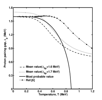
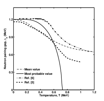
Figure 2: Temperature dependence of gap parameter in ${}^{94}Mo$ nucleus for the proton and the neutron system.

The values of the gap parameter at $T=0$ are $\Delta_{0p}=1.6Mev$ and $\Delta_{0n}=1.2Mev$ kke . which are used to calculate the interaction strength, $G$, by solving the gap equation (4) and equation (5) for protons and neutrons at zero temperature. In order to calculate $P(\Delta)$ as a function of temperature for both types of particles, particle number constraint, equation (11) is used. The results for neutrons in ${}^{94}Mo$ nucleus are given in fig.(1) in which $P(\Delta)$ is normalized. As it is seen its shape changes from symmetric Gaussian at temperatures lower than critical temperature $T_{c}=0.72MeV$, the temperature in which gap parameter becomes zero, We have extracted the following values of pairing gap at zero temperature, $\Delta_{0}$ for protons and neutrons, using the three point method pm to asymmetric shape at temperatures higher than $T_{c}$. In all temperatures the maximum value of $P(\Delta)$ is consistent with that of the most probable values. The resulted values of $\Delta$ versus temperature for protons and neutrons in ${}^{94}Mo$ nucleus are plotted in fig.(2). We have extracted the following values of pairing gap at zero temperature, $\Delta_{0}$ for protons and neutrons, using the three point method pm

$$\Delta_{0p}=1.7Mev \Delta_{0n}=1.15Mev$$ ; (17)

The results are also shown in fig.(2). The effect of different values of $\Delta_{0}$ on heat capacity will be discussed. The gradual decreasing of gap parameter with a sudden decrease is seen which can be comparable with the experimental values kk . The results obtained by K. Kaneko et.al,kke , are also shown for comparison. This is interpreted as a rapid breaking of nucleon Cooper pairs and the suppression of pairing correlation. Also this is correlated with the S shape of the heat capacity.

\begin{picture}(210.0,100.0)\put(0.0,-40.0){ \epsfbox{4.eps} } \end{picture}

Figure 3: Total energy versus temperature using the most and mean probable gap parameter in ${}^{94}Mo$ nucleus.

The mean gap parameter $\bar{\Delta}$ and its partial derivatives were applied to calculate energy as a function of temperature using equation(12) the total energy is $E=E_{n}+E_{p}$. The results are plotted in fig.(3) in comparison with the most probable energy from equation(6). This figure shows how using the mean value of the gap parameter leads to the smooth behavior of the energy near the critical temperature.

\begin{picture}(210.0,150.0)\put(0.0,-40.0){ \epsfbox{5.eps} } \end{picture}

Figure 4: Heat capacity as a function of temperature using the most and the mean probable gap parameter in ${}^{94}Mo$ nucleus.

\begin{picture}(210.0,150.0)\put(0.0,-40.0){ \epsfbox{6.eps} } \end{picture}

Figure 5: Heat capacity versus temperature using the mean probable gap parameter in ${}^{94}Mo$ nucleus. The experimental values and the calculated values from SPA and RPA+SPA methods(dashed and dotted-dashed lines, respectively, taken from kk ) are also plotted for comparison.

Based on the mean gap parameter, the heat capacity is calculated using equation (14). The results are plotted in fig.(4), for ${}^{94}Mo$ nucleus, for the two sets of $\Delta_{0}$, where $C=C_{n}+C_{p}$. Also in fig.(5) the experimental kke and the RPA+SPA heat capacities kk are plotted for comparison. The extracted results show the discontinuities have been disappeared and the heat capacity exhibits an S shape, very similar in shape with the experiments above $0.4MeV$. Below $0.5MeV$, the results of SPA, the NPSPA and this work are in coincidence.

In summery, taking into account thermal fluctuation, the discontinuity of the heat capacity is washed out and a continues S-shape around the critical temperature has been obtained as it is found experimentally kke . The S shape of the heat capacity is well correlated in temperature with the suppression of $\Delta_{p}$ and $\Delta_{n}$ as is shown in fig.(2). This is interpreted as a signature of the thermal pairing phase transition.

References

- (1) H. J. Lipkin, Ann of phys.9. 272(1960)
- (2) Y. Nogami, phys. Rev. B313. 134 (1964)
- (3) H. C. Pradhan, Y. Nogami and J.law, Nucl. phys. A201. 357 (1973)
- (4) R. Rossignoli, N. Canosa and P. Ring, Phys. Rev. Lett. 80. 9 (1990)
- (5) K. Kaneko and A. Shiller, Phys. Rev. C76. 064306 (2007)
- (6) K. Kaneko et al, Phys. Rev. C74. 024325 (2006)
- (7) L. D. Landau and E. M. Lifshitz, ”Statistical Physics” (Addision and Wesley, 1966) P. 348
- (8) L. G. Moretto, Phys. Lett. 1,40B (1972)
- (9) J. Bardeen, L. N. Cooper and J. R. Schrieffer, Phys. Rev. 108. 1175 (1957)
- (10) L. G. Moretto, Nucl. Phys. A185. 145 (1972)
- (11) S. G. Nilsson et al, Mat. Fys. Medd. K. Dan. Vidensk. Selsk. 32. 16 (1961)
- (12) P. Moller and I. R. Nix, Nucl. Phys. A 536,20 (1992)