Squeezing light with Majorana fermions

Abstract

Coupling a semiconducting nanowire to a microwave cavity provides a powerfull means to assess the presence or absence of isolated Majorana fermions in the nanowire. These exotic bound states can cause a significant cavity frequency shift but also a strong cavity nonlinearity leading for instance to light squeezing. The dependence of these effects on the nanowire gate voltages gives direct signatures of the unique properties of Majorana fermions, such as their self-adjoint character and their exponential confinement.

I Introduction

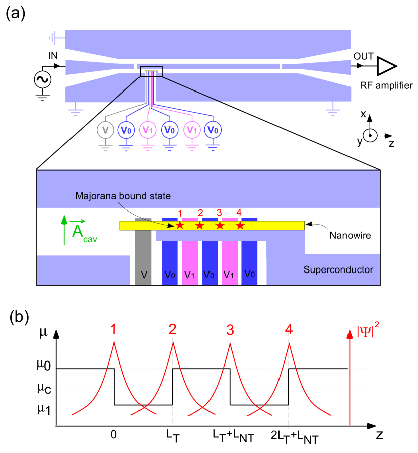
Figure 1: a. Scheme our our setup. The microwave cavity is made from the various superconducting contacts in purple. The nanowire (yellow) is placed between the center and ground conductors of the cavity. It is tunnel contacted to a grounded superconducting contact (purple) and capacitively contacted to three gate electrodes with voltage $V_{0}$ (blue) and two gate electrodes with voltage $V_{1}$ (pink) used to impose chemical potentials $\mu_{0}$ and $\mu_{1}$ in different sections of the nanowire. A normal metal contact (grey) with bias voltage $V$ is tunnel contacted to the nanowire to perform a conductance spectroscopy. b. Chemical potential (left axis) and schematic quasiparticle density probability (right axis) in the nanowire, versus coordinate $z$. Four MBSs appear at the boundaries between the topological ($\mu=\mu_{1}$) and non-topological ($\mu=\mu_{0}$) sections of the nanowire. In a finite length system, the MBSs wavefunctions overlap.

The observation of isolated Majorana fermions in hybrid nanostructures is one of the major challenges in quantum electronics. These elusive quasiparticles borrowed from high energy physics have the remarkable property of being their own antiparticleMajorana . They are expected to appear as zero energy localized modes in various types of heterostructuresreviews . One promising strategy is to use semiconducting nanowires with a strong spin-orbit coupling, such as InAs and InSb nanowires, placed in proximity with a superconductor and biased with a magnetic field Lutchyn ; Oreg . Most of the recent experiments proposed and carried out have focused on electrical transport which appears as the most natural probe in electronic devicesLutchyn ; Oreg ; Bolechetc ; Flensberg . While signatures consistent with the existence of Majorana fermions have been observed recentlyMouriketc , it is now widely accepted that alternative interpretations can explain most of the experimental findings observed so farLee ; Liu ; Pikulin ; Rainis ; Zareyan ; CottetSF ; Sau . One has therefore to do more than the early transport experiments to demonstrate unambiguously the existence of Majorana particles in condensed matter. Here, we propose to use the tools of cavity quantum electrodynamics to perform this task. Photonic cavities, or generally harmonic oscillators, are extremely sensitive detectors which can be used to probe fragile light-matter hybrid coherent statesWallraff:04 , non-classical light or even possibly gravitational wavesClerk . We show here that a photonic cavity can also be used to detect Majorana fermions and test their unique properties.

Recent technological progress has enabled the fabrication of nanocircuits based for instance on InAs nanowires inside coplanar microwave cavitiesDelbecq ; DQD ; Petersson . On the theory side, it has been suggested to couple nanowires to cavities to produce Majorana polaritons Trif , or build qubit architecturesTrif2 . Here, we adopt a different perspective which is the direct characterization of Majorana bound states (MBSs) through a photonic cavity. We consider a nanowire with four well defined Majorana bound states (MBSs), away from the nanowire topological transition. We find that these MBSs can be strongly coupled to the cavity when their spatial extension is large enough. When the four MBSs are coupled to the cavity, this leads to a transverse coupling scheme which induces a cavity frequency shift but also strong nonlinearities in the cavity behavior, such as light squeezingOng ; Kirchmair . Using electrostatic gates, it is possible to reach a regime where only two MBS remain coupled to the cavity. In this case, the cavity frequency shift and nonlinearity disappear. This represents a direct signature of the particle/antiparticle duality of MBSs. Indeed, the self-adjoint character of MBSs forces a longitudinal coupling to the cavity when only two MBSs are coupled to the cavity. The evolution of the cavity frequency shift and nonlinearity with the nanowire gate voltages furthermore enables an almost direct observation of the exponential localization of MBSs.

This article is organized as follows. In section II, we present the low-energy Hamiltonian model of the 4 Majorana nanowire considered in this article. In section III, we discuss the tunnel spectroscopy of this nanowire, through a normal metal contact placed close to one of the Majorana bound states. In section IV, we discuss the coupling between the nanowire and a microwave cavity. In section V, we discuss the behavior of the microwave cavity in the dispersive regime where the Majorana system and the cavity are not resonant. In section VI we discuss various simplifications used in our approach. Section VII concludes. For clarity, we have postponed various technical details and calculations to appendices. Appendix A presents a one-dimensional microscopic description of the nanowire, used to obtain the parameters occurring in the low energy Hamiltonian of section II and the coupling between the nanowire and the cavity used in section IV. Appendix B gives details on the calculation of the nanowire conductance. Appendix C discusses the behavior of the cavity in the classical regime, i.e. when a large number of photons are present in the cavity.

II Low-energy Hamiltonian model of the four Majorana nanowire

We consider a single channel nanowire subject to a Zeeman splitting $E_{z}$ and an effective gap $\Delta$ induced by a superconducting contact (Fig.1.a). The nanowire presents a strong Rashba spin-orbit coupling with a characteristic speed $\alpha_{so}$. The chemical potential $\mu$ in the nanowire can be tuned locally by using electrostatic gates. The details of the model are given in appendix A. For brevity, in this section, we discuss only the main features of the model which lead us to the effective low energy Hamiltonian used in the main text (Eqs.(1) and (2)). We note $\mu_{c}=\sqrt{E_{z}^{2}-\Delta^{2}}$ the chemical potential below which the wire is in a topological phaseLutchyn ; Oreg . The wire has two topological regions $\mu=\mu_{1}<\mu_{c}$ with length $L_{T}$ surrounded by three non topological regions $\mu=\mu_{0}>\mu_{c}$, with $L_{NT}$ the length of the central non topological region (Fig.1.b). MBSs appear in the nanowire at the interfaces between topological and non topological phases, for coordinates $z\simeq z_{i}$ with $i\in\{1,2,3,4\}$, $z_{1}=0$, $z_{2}=L_{T}$, $z_{3}=L_{T}+L_{NT}$, and $z_{4}=L_{NT}+2L_{T}$. In the topological phases, the wavefunction corresponding to MBS $i$ decays exponentially away from $z=z_{i}$ with the characteristic vector $k_{m}(\mu_{1})=(\Delta-\sqrt{E_{z}^{2}-\mu_{1}^{2}})/\hbar\alpha_{so}<0$ (see Appendix A for details). In the non-topological phases, the decay of the MBSs is set by the two characteristic vectors $k_{p/m}(\mu_{0})=(\Delta\pm\sqrt{E_{z}^{2}-\mu_{0}^{2}})/\hbar\alpha_{so}>0$. The difference in the number of characteristic vectors from the topological to the non-topological phases is fundamentally related to the existence of the topological phase transition in the nanowire. Away from the topological transition, one can introduce a Majorana fermionic operator $\gamma_{i}$ such that $\gamma_{i}^{{\dagger}}=\gamma_{i}$ and $\gamma_{i}^{2}=1/2$ to describe MBS $i$.

In a real system, due to the finite values of $L_{T}$ and $L_{NT}$, the different MBSs overlap. The resulting coupling can be described with the low energy Hamiltonian:

$$H_{wire}=2i\epsilon(\gamma_{1}\gamma_{2}+\gamma_{3}\gamma_{4})+2i\widetilde{\epsilon}\gamma_{2}\gamma_{3}$$ (1)

with $\epsilon\simeq\lambda_{\epsilon}e^{k_{m}(\mu_{1})L_{T}}$ and $\widetilde{\epsilon}\simeq\lambda_{\widetilde{\epsilon}}e^{-k_{m}(\mu_{0})L_{NT}}$. Note that $\epsilon$ and $\widetilde{\epsilon}$ are purely real because the Majorana operators are self-adjoint and $H$ must be Hermitian.  The coefficients $\lambda_{\epsilon}$ and $\lambda_{\widetilde{\epsilon}}$ depend on $\mu_{0}$, $\mu_{1}$, $E_{z}$ and $\Delta$ (see Appendix A.5). Importantly, the coupling energies $\epsilon$ and $\widetilde{\epsilon}$ depend exponentially on $L_{T}$ and $L_{NT}$, as a direct consequence from the exponentially localized nature of MBSs. Furthermore, the vectors $k_{m}(\mu_{1})$ and $k_{m}(\mu_{0})$ vanish for $\mu_{1}=\mu_{c}$ and $\mu_{0}=\mu_{c}$, respectively, or in other terms the spatial extension of the MBSs increases when one approaches the topological transition. In this limit, large values of $\epsilon$ and $\widetilde{\epsilon}$ can be obtained. However, it should be noted that the use of Eq.(1) is justified provided the nanowire is operated far enough from the topological transition. We have checked that this is the case for the parameters used in Figs. 2 and 5. This point will be discussed in more details in section VI.

III Tunnel spectroscopy of the nanowire

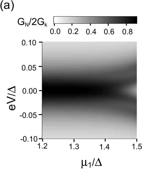
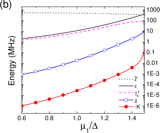
Figure 2: a. Conductance $G_{N}$ between the normal metal contact and the ground, versus the bias voltage $V$ and the chemical potential $\mu_{1}$. b. Coupling energies $\varepsilon$ and $\tilde{\varepsilon}$ (full and dotted black lines), transverse coupling $\gamma_{e}^{t}$ (pink dashed line), dispersive shift $\chi$ of the cavity frequency (blue line with open circles), and Kerr nonlinearity $K$ (red line with full circles) versus $\mu_{1}$. In this figure, we have used $\Delta=500~{}\mathrm{\mu eV}$, $E_{z}/\Delta=2$, $\mu_{0}/\Delta=1.9$, $\alpha_{so}\sim 8.10^{4}m.s^{-1}$, $L_{T}=L_{NT}=1000~{}\mathrm{nm}$, $\alpha_{c}V_{rms}=4~{}\mathrm{\mu V}$, $\omega_{cav}/2\pi=8~{}\mathrm{GHz}$, $\Gamma=2~{}\mathrm{\mu eV}$, $T=10~{}\mathrm{mK}$ and $G_{k}=e^{2}/h$. The topological transition is located well outside the $\mu_{1}$ range considered here since $\mu_{c}/\Delta=1.73$.

The simplest idea to probe MBSs is to perform a tunnel spectroscopy of the nanowire by placing a normal metal contact biased with a voltage $V$ on the nanowire, close to MBS 1 for instance (Fig.1.a). A current can flow between the normal metal contact and the ground, through the MBSs and the grounded superconducting contact shown in Fig.1a., which is tunnel coupled to the nanowire. To describe the main properties of the conductance $G_{N}$ between the normal metal contact and the ground, it is sufficient to assume an energy independent tunnel rate $\Gamma$ between MBS 1 and the contact. The details of the calculation are presented in appendix B. Figure 2.a shows $G_{N}$ as a function of $\mu_{1}$ and $V$, for realistic parameters (see legend of Fig.2). For $\mu_{0}$ and $\mu_{1}$ relatively close to $\mu_{c}$, $\epsilon$ and $\widetilde{\epsilon}$ can be comparable or larger than $\Gamma$ and the temperature scale $k_{B}T$. Hence, four conductance peaks appear at voltages corresponding to the eigenenergies $(\pm\hbar\omega_{e}\pm\hbar\omega_{o})/2$ of $H_{wire}$, with $\hbar\omega_{e}=2\sqrt{4\epsilon^{2}+\widetilde{\epsilon}^{2}}$ and $\hbar\omega_{o}=2\widetilde{\epsilon}$. In this regime, the current flows through the four MBSs which are coupled together, as represented in Fig.3.a. As $\mu_{1}$ decreases, the coupling between MBS 1 and the other MBSs

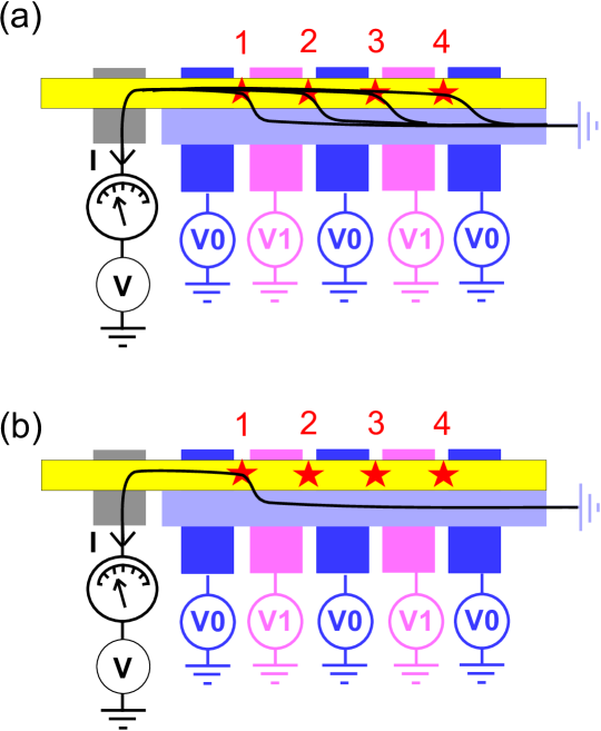
Figure 3: Schematic representation of the current flow in the nanocircuit depending on the value of $\mu_{1}$. Panel (a) corresponds to $\mu_{0}$ and $\mu_{1}$ close to $\mu_{c}$ so that $\varepsilon$ and $\widetilde{\varepsilon}$ are finite and the four MBSs are coupled together. In this regime the current flows from the superconducting contact (purple) to the normal metal contact (grey) through the four Majorana bound states. Panel (b) corresponds to a value of $\mu_{1}$ far below $\mu_{c}$ so that the coupling $\varepsilon$ between MBS1 and other MBSs vanishes.  In this case, the current flows from the superconducting contact to the normal metal contact through MBS 1 only.

disappear ($\epsilon\rightarrow 0$), so that there remains only a zero energy conductance peak which is due to transport through MBS 1, as represented in Fig.3.b. Similar features can be caused by other effects such as weak antilocalization, Andreev resonances or a Kondo effectLee ; Liu ; Pikulin ; Rainis ; Zareyan ; CottetSF . It is therefore important to search for other ways to probe MBSs more specifically. We show in the following that coupling the nanowire to a photonic cavity can give direct signatures of the self-adjoint character of MBSs and their exponential confinement. In the rest of the paper, we omit the explicit description of the normal metal contact. The Majorana system could be affected by decoherence, due to the normal metal contact or background charge fluctuators in the vicinity of the nanowire, for instance. However the detection scheme we present below is to a great extent immune to decoherence because it leaves the Majorana system in its ground state (we use $\hbar\omega_{e/o}\gg k_{B}T$).

IV Coupling between the nanowire and a microwave cavity

We assume that the nanowire is placed between the center and ground conductors of a coplanar waveguide cavity (Fig.1.a). We take into account a single mode of the cavity, corresponding to a photon creation operator $a^{{\dagger}}$. There exists a capacitive coupling between the nanowire and the cavity, which is currently observed in experimentsDelbecq ; DQD ; Petersson . More precisely, the nanowire chemical potential is shifted by $\mu_{ac}=e\alpha_{c}V_{rms}(a+a^{{\dagger}})$, with $V_{rms}$ the rms value of the cavity vacuum voltage fluctuations and $\alpha_{c}$ a capacitive ratio. This leads to the system Hamiltonian

$$H=H_{wire}+h_{int}(a+a^{{\dagger}})+\hbar\omega_{cav}a^{{\dagger}}a$$ (2)

with $h_{int}=2i\beta(\gamma_{1}\gamma_{2}+\gamma_{3}\gamma_{4})+2i\widetilde{\beta}\gamma_{2}\gamma_{3}$, $\beta\simeq\lambda_{\beta}(L_{T}/l_{c})\epsilon$, $\widetilde{\beta}\simeq\lambda_{\widetilde{\beta}}(L_{NT}/l_{c})\widetilde{\epsilon}$ and $l_{c}=\hbar\alpha_{so}/e\alpha_{c}V_{rms}$. Note that $\beta$ and $\widetilde{\beta}$ are purely real, due again to $\gamma_{i}^{{\dagger}}=\gamma_{i}$. The coefficients $\lambda_{\beta}$ and $\lambda_{\widetilde{\beta}}$ depend on $\mu_{0(1)}$ and $E_{z}$ (see appendix A.5). The term in $h_{int}$ is caused by the potential shift $\mu_{ac}$. Due to $h_{int}$, cavity photons modify the coupling between MBSs, as represented schematically in Fig.4.

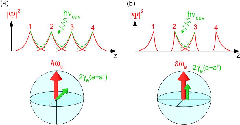
Figure 4: Schematic representation of the coupling mechanism between MBSs and cavity photons a. When $\mu_{0}$ and $\mu_{1}$ are close to the critical potential $\mu_{c}$, cavity photons modify the coupling between all consecutive MBSs. This yields a coupling between the nanowire and the cavity with a transverse component in the MBSs even charge sector, represented here on a Bloch sphere. b. When $\mu_{1}$ is far below $\mu_{c}$, only MBSs 2 and 3 remain coupled by cavity photons. In this case one can only have a longitudinal coupling in the nanowire even charge sector, as a direct consequence of the self-adjoint character of Majorana fermion operators.

Remarkably, $h_{int}$ has a form similar to $H_{wire}$, with coefficients $\beta$ and $\widetilde{\beta}$ containing the same exponential dependence on $L_{T}$ and $L_{NT}$ as $\epsilon$ and $\widetilde{\epsilon}$, because $\mu_{ac}$ is spatially constant along the nanowire. Hence, the amplitude of $h_{int}$ directly depends on the MBSs exponential overlaps.

One can reveal important properties of MBSs by varying $\mu_{1}$, with $\mu_{0}$ constant. Let us assume that $\mu_{0}$ is relatively close to $\mu_{c}$ so that $\widetilde{\epsilon}$ and $\widetilde{\beta}$ can be considered as finite. When $\mu_{1}$ is also close to $\mu_{c}$, $\epsilon$ and $\ \beta$ are finite, and in general $\beta\widetilde{\epsilon}\neq\widetilde{\beta}\epsilon$, so that $h_{int}$ and $H_{wire}$ are not proportional. This enables the existence of a transverse coupling between the Majorana system and the cavity, i.e. the cavity photons can induce changes in the state of the Majorana system, as we will see in more details below. In contrast, for $\mu_{1}$ far below $\mu_{c}$, $\epsilon$ and $\beta$ vanish because MBSs are strongly localized in the topological phases. This means that MBSs 2 and 3 remain coupled together and they are also coupled to the cavity, but MBSs 1 and 4 become isolated and thus irrelevant for the cavity (Fig 4.b). In this limit, $H$ takes the form of the Hamiltonian of a single pair of coupled Majorana fermions, i.e.

$$H^{\prime}\simeq 2i\widetilde{\epsilon}\gamma_{2}\gamma_{3}+2i\widetilde{\beta}\gamma_{2}\gamma_{3}(a+a^{{\dagger}})$$ (3)

Note that the eigenvalues of $H^{\prime}$ have a twofold degeneracy due to the existence of the isolated MBSs 1 and 4. Both terms in the Hamiltonian (3) have the same structure, or in other terms $h_{int}$ and $H_{wire}$ are proportional, due to constraints imposed by the self-adjoint character of Majorana fermions. Indeed, a quadratic Hamiltonian involving only MBSs 2 and 3 must necessarily be proportional to $i\gamma_{2}\gamma_{3}$ since the terms $\gamma_{2}^{{\dagger}}\gamma_{2}$ and $\gamma_{3}^{{\dagger}}\gamma_{3}$ are proportional to the identity and therefore inoperant for self-adjoint fermions. As a result, the coupling between the cavity and the Majorana system becomes purely longitudinal, as discussed in more details below.

To discuss more precisely the structure of the coupling between the nanowire and the cavity, it is convenient to reexpress $H$ in terms of ordinary fermionic operators. One possibility is to use the two fermions $c_{L}^{{\dagger}}=(\gamma_{1}-i\gamma_{2})/\sqrt{2}$ and $c_{R}^{{\dagger}}=(\gamma_{3}-i\gamma_{4})/\sqrt{2}$. A second possibility is to use $c_{m}^{{\dagger}}=(\gamma_{2}-i\gamma_{3})/\sqrt{2}$  and $c_{e}^{{\dagger}}=(\gamma_{1}-i\gamma_{4})/\sqrt{2}$. Depending on the cases, it is more convenient to use the first or the second possibility. We also define the occupation numbers $n_{f}=c_{f}^{{\dagger}}c_{f}$, for $f\in\{L,R,e,m\}$. In the discussion following, we recover the fact that in a closed system made of several Majorana bound states, the parity of the total number of fermions is conservedreviews . Note that in our system, the total fermions numbers $N_{tot}=n_{L}+n_{R}$ or $N_{tot}^{\prime}=n_{e}+n_{m}$ are not equivalent since they do not commute, but their parity $P=-4\gamma_{1}\gamma_{2}\gamma_{3}\gamma_{4}$ is the same.

For $\mu_{1}$ far below $\mu_{c}$, it is convenient to use the basis of the fermions $e$ and $m$ to reexpress the Hamiltonian as

$$H^{\prime}=(\widetilde{\epsilon}+\widetilde{\beta}(a+a^{{\dagger}}))(2n_{m}-1)+\hbar\omega_{cav}a^{{\dagger}}a$$ (4)

One can note that $c_{e}^{{\dagger}}$ and $c_{e}$ do not occur in $H^{\prime}$, therefore the $e$ fermionic degree of freedom can be disregarded. Moreover, one has $[H,n_{m}]=0$, which means that the number of fermions of type $m$ (or equivalently the parity of $n_{m}$) is a conserved quantity, as expected for an (effective) system of 2 Majorana bound states. Hence, the coupling to the cavity cannot change $n_{m}$, or in other terms it cannot affect the state of the Majorana fermions. This means that in this limit, the coupling between the nanowire and the cavity can only be longitudinal as already mentioned above.

When $\mu_{0}$ and $\mu_{1}$ are both close enough to $\mu_{c}$, it is more convenient to use the basis of fermions $L$ and $R$. We define $(0,0)=\left|0\right\rangle$, $(1,0)=c_{L}^{{\dagger}}\left|0\right\rangle$, $(0,1)=c_{R}^{{\dagger}}\left|0\right\rangle$, and $(1,1)=c_{L}^{{\dagger}}c_{R}^{{\dagger}}\left|0\right\rangle$. Since $\epsilon$, $\beta$, $\widetilde{\epsilon}$ and $\widetilde{\beta}$ are finite, we have a fully effective four-Majorana system whose Hamiltonian writes:

$$H =2\left(\epsilon+\beta(a+a^{{\dagger}})\right)(n_{L}+n_{R}-1)$$ (5)

$$+\left(\widetilde{\epsilon}+\widetilde{\beta}(a+a^{{\dagger}})\right)\left(c_{L}^{{\dagger}}c_{R}-c_{L}c_{R}^{{\dagger}}+c_{L}^{{\dagger}}c_{R}^{{\dagger}}-c_{L}c_{R}\right)$$

$$+\hbar\omega_{cav}a^{{\dagger}}a$$

One can check from this equation that the parity of $N_{tot}=n_{L}+n_{R}$ is conserved as expected. However, since we have now 2 fermionic degrees of freedom fully involved in the Hamiltonian, we have to consider the two parity subspaces $\mathcal{E}_{e}=\{(0,0),(1,1)\}$ and $\mathcal{E}_{o}=\{(0,1),(1,0)\}$, each with a dimension 2. The conservation of the total fermion parity forbids transitions between $\mathcal{E}_{e}$ and $\mathcal{E}_{o}$, as can be checked from the structure of Eq. (5). However, nothing forbids the cavity to induce transitions inside each of the parity subspaces, as shown by the structure of the term in $\widetilde{\beta}$. Therefore, when the 4 Majorana states are effective, a transverse coupling between the nanowire and the cavity is possible.

To push further our analysis, it is convenient to introduce effective spin operators $\overrightarrow{\sigma}_{e}=\{\sigma_{e,X},\sigma_{e,Z}\}$ and $\overrightarrow{\sigma}_{o}=\{\sigma_{o,X},\sigma_{o,Z}\}$ operating in the subspaces $\mathcal{E}_{e}$ and $\mathcal{E}_{o}$ respectively, i.e. $\sigma_{e,z}=1-c_{L}^{{\dagger}}c_{L}-c_{R}^{{\dagger}}c_{R}$, $\sigma_{e,x}=c_{L}^{{\dagger}}c_{R}^{{\dagger}}-c_{L}c_{R}$, $\sigma_{o,z}=c_{L}^{{\dagger}}c_{L}-c_{R}^{{\dagger}}c_{R}$, and $\sigma_{o,x}=(c_{L}^{{\dagger}}c_{R}-c_{L}c_{R}^{{\dagger}}).$ For convenience we rotate the spin operators as $\tilde{\sigma}_{e,z}=(-2\epsilon\sigma_{e,z}-\widetilde{\epsilon}\sigma_{e,x})/\sqrt{4\epsilon^{2}+\widetilde{\epsilon}^{2}}$, $\tilde{\sigma}_{e,x}=(-\widetilde{\epsilon}\sigma_{e,z}+2\epsilon\sigma_{e,x})/\sqrt{4\epsilon^{2}+\widetilde{\epsilon}^{2}}$ and $\tilde{\sigma}_{o,z}=-\sigma_{o,x}$. We finally obtain

$$H_{wire}=(\hbar\omega_{e}\tilde{\sigma}_{e,z}+\hbar\omega_{o}\tilde{\sigma}_{o,z})/2$$ (6)

and

$$h_{int}=\gamma_{e}^{t}\tilde{\sigma}_{e,x}+\gamma_{e}^{l}\tilde{\sigma}_{e,z}+\gamma_{o}^{l}\tilde{\sigma}_{o,z}$$ (7)

with

$$\gamma_{o}^{l}=\widetilde{\beta}$$ (8)

$$\gamma_{e}^{l}=(4\beta\epsilon+\widetilde{\beta}\widetilde{\epsilon})/\sqrt{4\epsilon^{2}+\widetilde{\epsilon}^{2}}$$ (9)

and

$$\gamma_{e}^{t}=\frac{2\left(\beta\widetilde{\epsilon}-\widetilde{\beta}\epsilon\right)\left(\sqrt{4\epsilon^{2}+\widetilde{\epsilon}^{2}}-2\epsilon\right)}{\sqrt{32\epsilon^{4}+12\epsilon^{2}\widetilde{\epsilon}^{2}+\widetilde{\epsilon}^{4}-4\epsilon(4\epsilon^{2}+\widetilde{\epsilon}^{2})^{3/2}}}$$ (10)

These expressions show that the cavity couples longitudinally to the odd charge sector, whereas the coupling to the even charge sector can have a transverse component $\gamma_{e}^{t}$ because $\beta\widetilde{\epsilon}\neq\widetilde{\beta}\epsilon$ in general (Fig 4.a). The absence of transverse coupling in the odd charge sector is a consequence of the particular symmetries that we have assumed in our system, as will be discussed in section VI. For $\mu_{1}$ far below $\mu_{c}$, $\epsilon$ and $\beta$ vanish thus $H^{\prime}\simeq{\textstyle\sum\nolimits_{j\in\{e,o\}}}H_{j}$ with

$$H_{j}=\frac{\hbar\omega_{j}}{2}\tilde{\sigma}_{j,z}+\gamma_{j}^{l}(a+a^{{\dagger}})\tilde{\sigma}_{j,z}$$ (11)

Both terms in the expression (11) have the same structure in the effective spin space. Thus, we recover again the fact that the coupling between the Majorana system and the cavity becomes purely longitudinal for $\mu_{1}$ far below $\mu_{c}$. The cancellation of the transverse coupling between the nanowire and the cavity is fundamentally related to the self-adjoint character of MBSs which imposes the forms (3), or equivalently (4) or (11) in the case of a 2 Majorana system.

In conclusion, one can reveal important properties of MBSs by varying $\mu_{1}$, with $\mu_{0}$ constant. The vanishing of $\gamma_{e}^{t}$ for $\mu_{1}$ far below $\mu_{c}$ in spite of the fact that $\widetilde{\epsilon}$ and $\widetilde{\beta}$ remain finite represents a strong signature of the self-adjoint character of MBSs. In addition, probing the dependence of $\gamma_{e}^{t}$ on $\mu_{1}$ could reveal the exponential confinement of MBSs since for $\mu_{1}$ sufficiently below $\mu_{c}$, $\gamma_{e}^{t}\simeq 4(\beta\widetilde{\epsilon}-\widetilde{\beta}\epsilon)/\widetilde{\epsilon}$ scales with $e^{k_{m}(\mu_{1})L_{T}}$. Also note that, in principle, for $\mu_{0}$ and $\mu_{1}$ close enough to $\mu_{c}$, $\gamma_{e}^{t}$ can be large due to the large spatial extension of MBSs (see Fig.2.b). To test these properties, it is important to have an experimental access to $\gamma_{e}^{t}$. We show below that this is feasible due to the strong effects of $\gamma_{e}^{t}$ on the cavity dynamics.

V Behavior of the microwave cavity in the dispersive regime

In the dispersive (i.e. non resonant) regime, the transverse coupling $\gamma_{e}^{t}$ between the effective spin $\overrightarrow{\tilde{\sigma}}_{e}$ and the cavity allows for fast high order processes in which the population of the effective spin is changed virtually. This effect can be described by using an adiabatic elimination followed by a projection on the nanowire ground stateCohen-Tannoudji . This yields an effective cavity Hamiltonian:

$$H_{adiab}=\hbar\omega_{cav}a^{{\dagger}}a+\chi a^{{\dagger}}a+K(a^{{\dagger}})^{2}a^{2}+o(\gamma_{e}^{6})$$ (12)

with $\omega_{cav}$ the cavity frequency,

$$\chi=\left(2(\gamma_{e}^{t})^{2}\omega_{e}/(\omega_{cav}^{2}-\omega_{e}^{2})\right)+o(\gamma_{e}^{4})$$ (13)

$$K =d^{-1}(\gamma_{e}^{t})^{2}(\gamma_{e}^{l})^{2}\omega_{e}(8\omega_{cav}^{4}+20\omega_{e}^{4}-28\omega_{e}^{2}\omega_{cav}^{2})$$ (14)

$$+d^{-1}(\gamma_{e}^{t})^{4}\omega_{e}(8\omega_{cav}^{4}-6\omega_{e}^{4}+22\omega_{e}^{2}\omega_{cav}^{2})+o(\gamma_{e}^{6})$$

and $d=(\omega_{e}^{2}-\omega_{cav}^{2})^{3}(4\omega_{cav}^{2}-\omega_{e}^{2})$. The transverse coupling $\gamma_{e}^{t}$ causes a cavity frequency shift $\chi$ and a non-linear term proportional to $K$, similar to the Kerr term widely used in nonlinear optics. Figure 2.b illustrates that $\epsilon$, $\gamma_{e}^{t}$, $\chi$ and $K$ quickly vanish when $\mu_{1}$ goes far below $\mu_{c}$. In this limit, $\chi$ and $K$ both scale with $(\gamma_{e}^{t})^{2}$ because due to $\gamma_{e}^{t}\ll\gamma_{e}^{l}\sim\widetilde{\beta}$, the first contribution in Eq.(14) dominates $K$. For the realistic parameters used in this figure, $\chi$ varies from about $14~{}$MHz to $9~{}10^{-4}~{}$MHz. In practice, $\chi$ can be measured straightforwardly by measuring the response of the cavity to an input signal with a small power, for values down to $-10^{-3}~{}$MHz at least. The upper value $\chi\simeq 14~{}\mathrm{MHz}$ is comparable to what has been obtained with strongly coherent two level systems slightly off-resonant with a microwave cavityMajer . Having a significant Kerr nonlinearity is more specific to the ultra-strong spin/cavity coupling regime, which we obtain in our system because MBSs have a large spatial extension near the topological transition. In Fig.2.b, the Kerr constant $K$ varies from $-0.31~{}$MHz to $-10^{-6}~{}$MHz. The value $K=-0.31~{}$MHz is comparable to nonlinearities obtained recently with microwave resonators coupled to Josephson junctionsOng ; Kirchmair . However, it is important to notice that our $\chi$ and $K$ term have an approximate exponential dependence on $\mu_{1}$ due to the factor $e^{k_{m}(\mu_{1})L_{T}}$ appearing in $\gamma_{e}^{t}$, which is very specific to MBSs.

Figure 5 illustrates how to measure $K$ by probing the response of the cavity to an input microwave signal. We note $\gamma_{in/out}$ the photonic coupling rate between the input/output port and the cavity, and $\gamma$ the total decoherence rate of cavity photons. If $K$ is small, it can be revealed by applying to the cavity a steady signal which drives the resonator into a semi-classical regime Ong (see details in Appendix C). The semiclassical response of the cavity to a forward and backward sweep of $\omega_{RF}$ becomes hysteretic for a critical power $P_{in}^{c}=4\gamma p_{in}^{0}/3\sqrt{3}\left|K\right|$ which can be used to determine $\left|K\right|$, with $p_{in}^{0}=\hbar\omega_{cav}\gamma^{2}/2\gamma_{in}$ the single photon input powerYurke (Fig.5.a). Such a technique should allow one to observe MBSs relatively far from the topological transition, by using a high input power which compensates for the smallness of $K$. For the measurement of $\chi$, one does not benefit from such an advantage, hence we believe that the measurement of $K$ can enable one to follow the behavior of MBSs on a wider range of $\mu_{1}$. For the highest values of $K$, the classically-defined critical power $P_{in}^{c}$ is so small that the resonator is still in a quantum regime at this power. In this case one can directly observe the cavity nonlinearity with a low input power, by performing a tomographic measurement of the cavity Husimi Q-function $Q(\alpha)=Tr[\rho_{cav}(t)\left|\alpha\right\rangle\left\langle\alpha\right|]$ at a time $\Delta t$ after switching off the input biasKirchmair (Fig.5.b). Here $\rho_{cav}(t)$ is the cavity density matrix, $\left|\alpha\right\rangle=e^{-\left|\alpha\right|^{2}/2}{\textstyle\sum\nolimits_{n}}\alpha^{n}\left|n\right\rangle/\sqrt{n!}$ denotes a cavity coherent state and $\left|n\right\rangle$ a cavity Fock state with $n$ photons. The $K$ term can produce a strong photon amplitude squeezing which can be calculated for $\hbar\omega_{cav}\gg k_{B}T$ following Ref.Milburn .

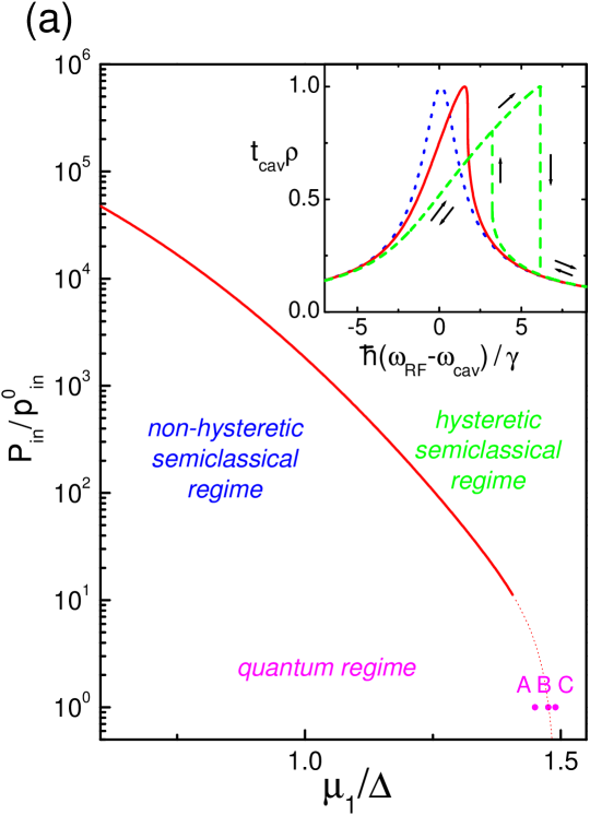
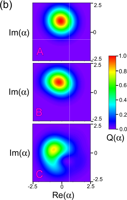
Figure 5: a. Diagram of the cavity behavior depending on the steady power $P_{in}$ applied to its input port and the nanowire potential $\mu_{1}$. For $P_{in}>P_{in}^{crit}$, the behavior of the cavity becomes hysteretic. Inset: Modulus $t_{cav}$ of the cavity transmission for a forward and backward sweep of $\omega_{RF}$, for $P_{in}=P_{in}^{crit}/4$ (blue dotted lines), $P_{in}=P_{in}^{crit}$ (full red lines) and $P_{in}=4P_{in}^{crit}$ (green dashed lines). b. Cavity Husimi function $Q(\alpha)$ at points A, B and C of Fig.4.a, at a time $\Delta t=175\mathrm{ns}$ after switching off an input power imposing a coherent cavity state $\left|i\right\rangle$. We have used the same parameters as in Fig.2, $\rho=\gamma/2\sqrt{\gamma_{in}\gamma_{out}}$ and $Q_{cav}=\hbar\omega_{cav}/2\pi\gamma=10000$.

VI Discussion

Before concluding, we discuss various simplifications used in the description of our results. First, we find that the nanowire odd charge sector does not have a transverse coupling to the cavity due to the symmetry between the sections 1-2 and 3-4 of the nanowire. If these sections had different lengths or parameters, a coupling to the odd charge sector would be possible, but we expect qualitatively similar results in this case because in the limit of $\mu_{1}$ far below $\mu_{c}$, the self-adjoint character of Majorana operators still imposes a system Hamiltonian of the form (3), or equivalently (4) or (11), and the coupling between MBSs 1 and 2 (3 and 4) should still depend exponentially on $L_{T}$. Second, with our nanowire model, a topological transition also occurs for $\mu=-\mu_{c}$. Therefore, upon decreasing $\mu$ the absolute values of $\epsilon$, $\beta$, $\gamma_{e}^{t}$, $\chi$ and $K$ reach minima for $\mu\sim 0$, and increase again when $\mu_{1}$ approaches $-\mu_{c}$. We have not discussed this limit because it gives results similar to $\mu\rightarrow\mu_{c}$.

Note that the use of the low energy Hamiltonian description, i.e. Eqs.(1) and (2), is justified provided the nanowire is operated far enough from the topological transition. This is essential to have large enough nanowire bandgaps. These bandgaps can be defined as $E_{b}^{1(0)}=(2\Delta^{2}+\mu_{1(0)}^{2}+\mu_{c}^{2}-2((\Delta^{2}+\mu_{1(0)}^{2})(\Delta^{2}+\mu_{c}^{2}))^{1/2})^{1/2}$ in the topological (non-topological) sections of the nanowire. With the parameters range considered in Figs. 2 and 4, one has $E_{b}^{1(0)}>35.6~{}\mathrm{GHz}$. In comparison, our hybridized Majorana bound states lie at frequencies $\pm\omega_{e}/2\pm\omega_{o}/2$ which lie in the interval $[-2.4~{}\mathrm{GHz}$, $2.4~{}\mathrm{GHz}]$. Therefore, these bound states are well separated from the continuum of states which exists above the nanowire gaps. With a typical cavity ($\omega_{cav}=8~{}\mathrm{GHz}$), it is thus not possible to excite quasiparticle above these gaps. Operating the device away from the topological transition also grants that possible fluctuations of the nanowire potentials due to charge fluctuators in the environment of the nanowire will not be harmful. For the range of parameters considered in Figs. 2 and 4, one has $\mid\mu_{0(1)}-\mu_{c}\mid>84~{}\mathrm{\mu eV}>eV_{ch}$, with $V_{ch}\simeq 10~{}\mathrm{\mu V}$ the typical amplitude for charge noise in semiconducting nanowires (see Ref. Petersson ). Charge noise is a low frequency effect which should mainly smooth the measured $\chi$ and $K$ if one stays away from the topological transition. This effect should not be dramatic since we expect the exponential variation of $\chi$ and $K$ to occur on a wide $\mu_{1}$ potential scale.

In more sophisticated models including disorder or several channels, the occurrence of MBSs can be more complex (see e.g. Pikulin ; Liu ; Brouwer ; Potter ; Lim ). Our setup precisely aims at testing whether their exists regimes where the four-MBSs low energy description of Eqs.(1) and (2) remains valid. In this limit, our findings are very robust since they only rely on the fact that MBS have a self-adjoint character and a gate-controlled spatial extension. Interestingly, a double quantum dot (DQD) can also be coupled transversely to a microwave cavityDQDth , which leads to a cavity frequency shift, as confirmed by recent experiments DQD ; Petersson . When the double dot and the cavity are coupled dispersively, and the two dot orbitals resonant, the cavity frequency shift and the DQD conductance are maximal. However, when the DQD orbital energies or interdot hopping are varied to decrease the cavity frequency shift, this also switches off the DQD conductance. In contrast, for the system we consider here, the low energy conductance peak will persist in spite of the decrease of $\chi$ and $K$. Hence, it can be useful to measure simultaneously the cavity response and the nanosystem conductance to discard spurious effects due to accidental quantum dots. Note that this does not make our proposal more difficult to realize experimentally. Such joint measurements are currently performed in experiments combining nanocircuits and coplanar microwave cavities. This is a recent but mature technology as can been seen in Refs. Delbecq ; DQD ; Petersson .

VII Conclusion

In conclusion, we have considered a semiconducting nanowire device hosting four MBSs coupled to a microwave cavity. This systems shows a cavity frequency shift and a Kerr photonic nonlinearity when the nanowire is close enough to the topological transition. These effects disappear when the nanowire gates are tuned such that only two MBSs remain coupled to the cavity, due to the self-adjoint character of MBSs which imposes strong constraints on the cavity/nanowire coupling. Meanwhile, the low energy conductance peak caused by the MBSs persists, a behavior which should be difficult to mimic with other systems. The gate dependences of the cavity frequency shift and of the Kerr nonlinearity should furthermore reveal the exponential confinement of MBSs.

We acknowledge discussions with G. Bastard, R. Feirrera, B. Huard, F. Mallet, M. Mirrahimi and J.J. Viennot. This work was financed by the EU-FP7 project SE2ND[271554] and the ERC Starting grant CirQys.

VIII Appendix A: One dimensional microscopic description of the semiconducting nanowire

VIII.1 A.1 Initial one-dimensional Hamiltonian for the semiconducting nanowire

We describe the electronic dynamics in the nanowire with an effective one-dimensional Hamiltonian

$$\mathcal{H}_{1D}={\textstyle\int}dz[\begin{array}[c]{cc}\Psi_{\uparrow}^{{\dagger}}(z)&\Psi_{\downarrow}^{{\dagger}}(z)\end{array}]H_{1D}\left[\begin{array}[c]{c}\Psi_{\uparrow}(z)\\ \Psi_{\downarrow}(z)\end{array}\right]$$ (15)

with

$$H_{1D}(z) =-\frac{\hbar^{2}}{2m}\frac{\partial^{2}}{\partial z^{2}}+E_{z}\sigma_{z}-\mu(z)-\mu_{ac}$$

$$-i\hbar(\alpha_{x}\sigma_{y}-\alpha_{y}\sigma_{x})\frac{\partial}{\partial z}$$ (16)

Here, $\Psi_{\sigma}^{{\dagger}}(z)$ creates an electron with spin $\sigma$ at coordinate $z$. An external magnetic field induces a Zeeman splitting $E_{z}$ in the nanowire. The chemical potential $\mu(z)$ can be controlled by using electrostatic gates. The constants $\alpha_{x}$ and $\alpha_{y}$ account for Rashba spin-orbit interactions corresponding to an effective electric field which we express here in terms of a velocity vector $\overrightarrow{\alpha_{so}}=\alpha_{x}\overrightarrow{u_{x}}+\alpha_{y}\overrightarrow{u_{y}}$. The vector $\overrightarrow{\alpha_{so}}$ is expected to be perpendicular to the nanowireNadj . Such a model is suitable provided the description of the nanowire can be reduced to the lowest transverse channelLutchyn2 . We describe the coupling between the nanowire and the cavity by using a potential term

$$\mu_{ac}=e\alpha_{c}V_{rms}(a+a^{{\dagger}})$$ (17)

with $V_{rms}$ the rms value of the cavity vacuum voltage fluctuations and $\alpha_{c}$ a dimensionless constant which depends on the values of the different capacitances in the circuit. This type of coupling between a nanoconductor and a cavity has been observed experimentallyDelbecq ; DQD ; Petersson . In recent experiments, $\alpha_{c}\sim 0.3$ has been measuredDelbecq . Optimization of the microwave designs could be used to increase this value.

VIII.2 A.2 Bogoliubov-De Gennes equations for the nanowire

One can describe the superconducting proximity effect inside the nanowire by using

$$\mathcal{H}_{BCS}=\mathcal{H}_{1D}+{\textstyle\int}dz(\Delta\Psi_{\uparrow}^{{\dagger}}(z)\Psi_{\downarrow}^{{\dagger}}(z)+\Delta^{\ast}\Psi_{\downarrow}(z)\Psi_{\uparrow}(z))$$ (18)

with $\Delta$ a proximity-induced gap. We perform a Bogoliubov-De Gennes transformation

$$\gamma_{n}^{\dagger} ={\textstyle\int}dz^{\prime}(u_{\uparrow}(z^{\prime})\Psi_{\uparrow}^{{\dagger}}(z^{\prime})+u_{\downarrow}(z^{\prime})\Psi_{\downarrow}^{{\dagger}}(z^{\prime})$$

$$+v_{\uparrow}(z^{\prime})\Psi_{\uparrow}(z^{\prime})+v_{\downarrow}(z^{\prime})\Psi_{\downarrow}(z^{\prime}))$$ (19)

such that $\mathcal{H}_{BCS}=\sum_{n}E_{n}\gamma_{n}^{\dagger}\gamma_{n}$. The coefficients $u_{\uparrow}$, $u_{\downarrow}$, $v_{\uparrow}$ and $v_{\downarrow}$ can be obtained by solving

$$h_{eff}(z)\left[\begin{tabular}[c]{l}$u_{\uparrow}$\\ $u_{\downarrow}$\\ $v_{\downarrow}$\\ $-v_{\uparrow}$\end{tabular}\ \ \right]=E_{n}\left[\begin{tabular}[c]{l}$u_{\uparrow}$\\ $u_{\downarrow}$\\ $v_{\downarrow}$\\ $-v_{\uparrow}$\end{tabular}\ \ \ \ \right]$$ (20)

with

$$h_{eff}(z)=\left[\begin{array}[c]{cc}H_{1D}(z)&\Delta\sigma_{0}\\ \Delta^{\ast}\sigma_{0}&-\sigma_{y}H_{1D}^{\ast}(z)\sigma_{y}\end{array}\right]$$ (21)

Using the above expression of $H_{1D}(z)$, one gets

$$h_{eff}(z)=h_{W}(z)+h_{C}(z)$$ (22)

with

$$h_{W}(z) =\left(\frac{p_{z}^{2}}{2m}-\mu(z)+p_{z}\left(\alpha_{x}\sigma_{y}-\alpha_{y}\sigma_{x}\right)\right)\tau_{z}$$

$$-\Delta\tau_{x}+E_{z}\sigma_{z}$$ (23)

and

$$h_{C}(z)=-\mu_{ac}\tau_{z}$$ (24)

In the following we disregard the term in $p_{z}^{2}/2m$ because we look for solutions with a low $p_{z}$.

VIII.3 A.3 Expressing $h_{W}(z)$ in a purely imaginary basis

We define

$$\alpha_{x} =\alpha_{so}\cos(\theta_{so})$$ (25)

$$\alpha_{y} =\alpha_{so}\sin(\theta_{so})$$ (26)

In the following, we work at first order in $p_{z}$ because we are only interested in the low energy eigenstates of $h_{eff}(z)$. It is convenient to express $h_{eff}(z)$ in a basis of self-adjoint operators. For this purpose we define

$$R=\left[\begin{array}[c]{cccc}-\frac{i}{\sqrt{2}}e^{-\frac{i\theta_{so}}{2}}&\frac{1}{\sqrt{2}}e^{-\frac{i\theta_{so}}{2}}&0&0\\ 0&0&\frac{1}{\sqrt{2}}e^{\frac{i\theta_{so}}{2}}&-\frac{i}{\sqrt{2}}e^{\frac{i\theta_{so}}{2}}\\ 0&0&\frac{1}{\sqrt{2}}e^{-\frac{i\theta_{so}}{2}}&\frac{i}{\sqrt{2}}e^{-\frac{i\theta_{so}}{2}}\\ -\frac{i}{\sqrt{2}}e^{\frac{i\theta_{so}}{2}}&-\frac{1}{\sqrt{2}}e^{\frac{i\theta_{so}}{2}}&0&0\end{array}\right]$$ (27)

One can check

$$\widetilde{h}_{W}(z) =R^{-1}h_{W}(z)R$$

$$=\mu(z)\sigma_{y}\tau_{z}-i\hbar\alpha_{so}\tau_{x}\sigma_{z}\frac{\partial}{\partial z}-E_{z}\sigma_{y}+\Delta\tau_{y}$$ (28)

$$\widetilde{h}_{C}(z)=R^{-1}h_{C}(z)R=-e\alpha_{c}V_{rms}\tau_{z}\sigma_{y}(a+a^{{\dagger}})$$ (29)

Since $\widetilde{h}_{W}^{\ast}(z)=-\widetilde{h}_{W}(z)$ it is possible to impose to all the zero energy eigenvectors

$$\widetilde{\mathcal{\phi}}(z)=(u_{a}(z),u_{b}(z),u_{c}(z),u_{d}(z))^{t}$$ (30)

of $\widetilde{h}_{W}$ to be real. These eigenvectors correspond to operators

$$\gamma_{n}^{\dagger} ={\textstyle\int}dz^{\prime}(u_{a}(z^{\prime})\gamma_{a}(z^{\prime})+u_{b}(z^{\prime})\gamma_{b}(z^{\prime})$$

$$+u_{c}(z^{\prime})\gamma_{c}(z^{\prime})+u_{d}(z^{\prime})\gamma_{d}(z^{\prime}))$$ (31)

with

$$\gamma_{a}(z) =-\frac{i}{\sqrt{2}}e^{-\frac{i\theta_{so}}{2}}\psi_{\uparrow}^{{\dagger}}(z)+\frac{i}{\sqrt{2}}e^{+\frac{i\theta_{so}}{2}}\psi_{\uparrow}(z)=\gamma_{a}^{{\dagger}}(z)$$

$$\gamma_{b}(z) =\frac{1}{\sqrt{2}}e^{-\frac{i\theta_{so}}{2}}\psi_{\uparrow}^{{\dagger}}(z)+\frac{1}{\sqrt{2}}e^{+\frac{i\theta_{so}}{2}}\psi_{\uparrow}(z)=\gamma_{b}^{{\dagger}}(z)$$

$$\gamma_{c}(z) =\frac{1}{\sqrt{2}}e^{\frac{i\theta_{so}}{2}}\psi_{\downarrow}^{{\dagger}}(z)+\frac{1}{\sqrt{2}}e^{-\frac{i\theta_{so}}{2}}\psi_{\downarrow}(z)=\gamma_{c}^{{\dagger}}(z)$$

$$\gamma_{d}(z) =-\frac{i}{\sqrt{2}}e^{\frac{i\theta_{so}}{2}}\psi_{\downarrow}^{{\dagger}}(z)+\frac{i}{\sqrt{2}}e^{-\frac{i\theta_{so}}{2}}\psi_{\downarrow}(z)=\gamma_{d}^{{\dagger}}(z)$$

With this representation one can easily check that a zero energy normalized eigenvector of $\widetilde{h}_{W}(z)$ corresponds to a Majorana bound state (MBS) $\gamma_{n}^{\dagger}=\gamma_{n}$ with $\gamma_{n}^{2}=1/2$.

VIII.4 A.4 Eigenstates of $\widetilde{h}_{W}(z)$

VIII.4.1 Uniform case

In the case of a spatially constant $\mu$, assuming $\left|\mu\right|<E_{z}$, the zero energy eigenstates of $\widetilde{h}_{W}(z)$ are $V_{k_{m}}^{+}\exp(k_{m}z)$, $V_{k_{m}}^{-}\exp(-k_{m}z)$, $V_{k_{p}}^{+}\exp(k_{p}z)$, and $V_{k_{p}}^{-}\exp(-k_{p}z)$ with

$$k_{m}(\mu) =\frac{\Delta-\sqrt{E_{z}^{2}-\mu^{2}}}{\hbar\alpha_{so}}$$ (32)

$$k_{p}(\mu) =\frac{\Delta+\sqrt{E_{z}^{2}-\mu^{2}}}{\hbar\alpha_{so}}$$ (33)

$$V_{m}^{+}(\mu) =(-\cos\phi(\mu),0,0,\sin\phi(\mu))^{t}$$ (34)

$$V_{m}^{-}(\mu) =(0,\cos\phi(\mu),\sin\phi(\mu),0)^{t}$$ (35)

$$V_{p}^{+}(\mu) =(\cos\phi(\mu),0,0,\sin\phi(\mu))^{t}$$ (36)

$$V_{p}^{-}(\mu) =(0,-\cos\phi(\mu),\sin\phi(\mu),0)^{t}$$ (37)

and

$$\phi(\mu)=\arctan(\sqrt{\frac{E_{z}-\mu}{E_{z}+\mu}})$$ (38)

Note that in order to find the above solutions, we have assumed that the term in $p_{z}^{2}/2m$ is smaller than the other terms of the Hamiltonian (23). This is valid provided

$$2m\alpha_{so}^{2}\gg\frac{\left(\Delta-\sqrt{E_{z}^{2}-\mu^{2}}\right)^{2}}{\min(\mu,E_{z},\Delta,\Delta-\sqrt{E_{z}^{2}-\mu^{2}})}$$ (39)

and

$$2m\alpha_{so}^{2}\gg\frac{\left(\Delta+\sqrt{E_{z}^{2}-\mu^{2}}\right)^{2}}{\min(\mu,E_{z},\Delta)}$$ (40)

This criterion is largely satisfied in our work considering that the scale $2m\alpha_{so}^{2}$ is typically huge ($\sim 40~{}\mathrm{meV}$) in comparison with $\Delta$ and $E_{z}$ ($\sim 500~{}\mathrm{\mu eV}$).

VIII.4.2 Non-uniform case, disregarding finite size effects

In the main text, we study a nanowire with topological ($\mu=\mu_{1}<\mu_{c}$)  and non-topological ($\mu=\mu_{0}>\mu_{c}$) regions, with $\mu_{c}=\sqrt{E_{z}^{2}-\Delta^{2}}$ the chemical potential at which the bulk topological transition occurs. We consider the $\mu(z)$ profile of the main text, Figure 1.b. For $L_{T}\rightarrow+\infty$ and $L_{NT}\rightarrow+\infty$, one has four MBSs appearing at $z=0$, $z=L_{T}$, $z=L_{T}+L_{NT}$, $z=2L_{T}+L_{NT}$, with corresponding eigenfunctions $\widetilde{\mathcal{\phi}}_{i}(z)$ such that $\widetilde{h}_{W}(z)\widetilde{\mathcal{\phi}}_{i}(z)=0$, with $i\in\{1,2,3,4\}$. These four states correspond to the Majorana operators $\gamma_{1}$, $\gamma_{2}$, $\gamma_{3}$ and $\gamma_{4}$ of the main text. One can check, for MBS 1:

$$\widetilde{\mathcal{\phi}}_{1}(z <0)=\frac{\mathcal{N}}{2}\Omega_{+}V_{m}^{+}(\mu_{0})\exp(k_{m}(\mu_{0})z)$$

$$+\frac{\mathcal{N}}{2}\Omega_{-}V_{p}^{+}(\mu_{0})\exp(k_{p}(\mu_{0})z)$$ (41)

$$\widetilde{\mathcal{\phi}}_{1}(z>0)=\mathcal{N}V_{m}^{+}(\mu_{1})\exp(k_{m}(\mu_{1})z)$$ (42)

and for MBS 2:

$$\widetilde{\mathcal{\phi}}_{2}(z<L_{T})=\mathcal{N}V_{m}^{-}(\mu_{1})\exp(-k_{m}(\mu_{1})(z-L_{T}))$$ (43)

$$\widetilde{\mathcal{\phi}}_{2}(z >L_{T})=\frac{\mathcal{N}}{2}\Omega_{+}V_{m}^{-}(\mu_{0})\exp(-k_{m}(\mu_{0})(z-L_{T}))$$

$$+\frac{\mathcal{N}}{2}\Omega_{-}V_{p}^{-}(\mu_{0})\exp(-k_{p}(\mu_{0})(z-L_{T}))$$ (44)

The vectors $V_{p}^{\pm}(\mu_{1})$ do not occur in these solutions because their symmetry is not compatible with the solutions in the non-topological phase (assuming we keep only normalizable solutions)Lutchyn ; Oreg ; Sticlet . Similarly, one has, for MBS 3:

$$\widetilde{\mathcal{\phi}}_{3}(z)=\widetilde{\mathcal{\phi}}_{1}(z-L_{T}-L_{NT})$$ (45)

and for MBS 4:

$$\widetilde{\mathcal{\phi}}_{4}(z)=\widetilde{\mathcal{\phi}}_{2}(z-L_{T}-L_{NT})$$ (46)

We have used above:

$$\Omega_{\pm}=\frac{\sin\phi(\mu_{1})}{\sin\phi(\mu_{0})}\pm\frac{\cos\phi(\mu_{1})}{\cos\phi(\mu_{0})}$$ (47)

and the normalization factor:

$$\mathcal{N}=\sqrt{\frac{2\Delta\left(\Delta^{2}+\mu_{0}^{2}-E_{z}^{2}\right)\left(\sqrt{E_{z}^{2}-\mu_{1}^{2}}-\Delta\right)}{\hbar\alpha_{so}(\mu_{0}-\mu_{1})\left(\Delta\mu_{1}+\mu_{0}\sqrt{E_{z}^{2}-\mu_{1}^{2}}\right)}}$$ (48)

VIII.5 A. 5 Coupling between Majorana bound states for finite $L_{T}$ and $L_{NT}$

For finite values of $L_{T}$ and $L_{NT}$, we have to take into account a DC coupling $\alpha_{ij}={\textstyle\int}\widetilde{\mathcal{\phi}}_{i}(z)\widetilde{h}_{W}(z)\widetilde{\mathcal{\phi}}_{j}(z)$ between adjacent MBSs $i$ and $j$. We disregard the coupling between non-adjacent bound states which is expected to be weaker. We use a perturbation approach to calculate $\alpha_{ij}$, similar to Ref.Shivamoggi . We obtain the Hamiltonian $H_{wire}$ of the main text, with $\epsilon$ and $\widetilde{\epsilon}$ real constants given by $\alpha_{12}=\alpha_{34}=i\epsilon$ and $\alpha_{23}=i\widetilde{\epsilon}$. One can check $\epsilon\simeq\lambda_{\epsilon}e^{k_{m}(\mu_{1})L_{T}}$ and $\widetilde{\epsilon}\simeq\lambda_{\widetilde{\epsilon}}e^{-k_{m}(\mu_{0})L_{NT}}$ with

$$\lambda_{\epsilon}=2\zeta\sqrt{E_{z}^{2}-\mu_{1}^{2}}$$ (49)

$$\lambda_{\widetilde{\epsilon}}=\zeta\left(\sqrt{(E_{z}^{2}-\mu_{1}^{2})}+\left((E_{z}^{2}-\mu_{0}\mu_{1})/\sqrt{E_{z}^{2}-\mu_{0}^{2}}\right)\right)$$ (50)

and

$$\zeta=\Delta(\mu_{0}^{2}-\mu_{c}^{2})(\mu_{1}^{2}-\mu_{c}^{2})/(E_{z}(\mu_{1}-\mu_{0})\vartheta)$$ (51)

with

$$\vartheta=E_{z}^{2}\mu_{0}+\mu_{1}\Delta^{2}-\mu_{0}\mu_{1}^{2}+\Delta(\mu_{0}+\mu_{1})\sqrt{E_{z}^{2}-\mu_{1}^{2}}$$ (52)

The expression of $\widetilde{\epsilon}$ has been approximated using

$$\exp[-2L_{NT}\sqrt{E_{z}^{2}-\mu_{0}^{2}})/\hbar\alpha_{Z}]\ll 1$$ (53)

Cavity photons couple to MBSs due to $\widetilde{h}_{C}(z)$ defined in Eq.(29). Again, it is sufficient to consider the coupling between consecutive MBSs. The constants $\beta$ and $\widetilde{\beta}$ of the main text correspond to $\beta(a+a^{{\dagger}})={\textstyle\int}\widetilde{\mathcal{\phi}}_{1}(z)\widetilde{h}_{C}(z)\widetilde{\mathcal{\phi}}_{2}(z)$ and $\widetilde{\beta}(a+a^{{\dagger}})={\textstyle\int}\widetilde{\mathcal{\phi}}_{2}(z)\widetilde{h}_{C}(z)\widetilde{\mathcal{\phi}}_{3}(z)$. Using (53), one finds the Hamiltonian $h_{int}$ of the main text with

$$\beta\simeq\lambda_{\beta}\frac{L_{T}}{l_{c}}\epsilon$$ (54)

$$\widetilde{\beta}\simeq\left(\gamma_{\widetilde{\beta}}\frac{eV_{rms}}{\mu_{0}}+\lambda_{\widetilde{\beta}}\frac{L_{NT}}{l_{c}}\right)\widetilde{\epsilon}$$ (55)

$$\lambda_{\beta}=\frac{\mu_{1}}{\sqrt{E_{z}^{2}-\mu_{1}^{2}}}$$ (56)

$$\gamma_{\widetilde{\beta}} =\frac{E_{z}^{2}\mu_{0}(\mu_{1}-\mu_{0})}{(E_{z}^{2}-\mu_{0}^{2})(E_{z}^{2}-\mu_{0}\mu_{1}+\sqrt{(E_{z}^{2}-\mu_{0}^{2})(E_{z}^{2}-\mu_{1}^{2})})}$$ (57)

$$\lambda_{\tilde{\beta}} =\frac{\mu_{0}\left((E_{z}^{2}-\mu_{0}^{2})\sqrt{E_{z}^{2}-\mu_{1}^{2}}+(E_{z}^{2}-\mu_{0}\mu_{1})\sqrt{E_{z}^{2}-\mu_{0}^{2}})\right)}{(E_{z}^{2}-\mu_{0}^{2})(E_{z}^{2}-\mu_{0}\mu_{1}+\sqrt{(E_{z}^{2}-\mu_{0}^{2})(E_{z}^{2}-\mu_{1}^{2})})}$$ (58)

For the realistic parameters we consider, the dimensionless parameters $\lambda_{\beta}$, $\gamma_{\widetilde{\beta}}$ and $\lambda_{\widetilde{\beta}}$ are of the order of $1$ while $eV_{rms}/\mu_{0}\ll L_{NT}/l_{c}$. This leads to

$$\widetilde{\beta}\simeq\lambda_{\widetilde{\beta}}\frac{L_{NT}}{l_{c}}\widetilde{\epsilon}$$ (59)

IX Appendix B: Conductance of the Majorana nanowire

The ensemble of the nanowire and the normal metal contact connected to MBS 1 can be described by a Hamiltonian $H_{wire}+H_{N}$ withBolechetc

$$H_{N}={\textstyle\sum\limits_{p}}\varepsilon_{p}c_{p}^{{\dagger}}c_{p}+t(c_{p}^{{\dagger}}-c_{p})\gamma_{1}$$ (60)

For simplicity, we assume that the coupling element $t$ between MBS 1 and the contact is energy independent. Since the nanowire is tunnel coupled to a grounded superconducting contact, a current can flow between this superconducting contact and the normal metal contact, though the MBSs. The conductance of the contact can be calculated asFlensberg

$$G=(2e^{2}/h){\textstyle\int}d\varepsilon g_{0}(\varepsilon)\frac{df(\varepsilon-eV)}{d\varepsilon}$$ (61)

with $f(\varepsilon)=1+\exp(\varepsilon/k_{B}T)$ the Fermi function , $\Gamma=2\pi\nu_{0}\left|t\right|^{2}$ the tunnel rate to between the contact and MBS 1, $\nu_{0}$ the density of states in the contact and

$$g_{0}=\frac{\Gamma^{2}\omega^{2}(\omega^{2}-4(\epsilon^{2}+\widetilde{\epsilon}^{2}))^{2}}{\left|16\epsilon^{4}+4\epsilon^{2}(i\Gamma-2\omega)\omega+\omega(-i\Gamma+\omega)(\omega^{2}-4\epsilon^{2})\right|^{2}}$$ (62)

Near the topological transition ($\varepsilon$ and $\widetilde{\varepsilon}$ finite), and if $\Gamma$ and $k_{B}T$ are small, the conductance $G$ displays four peaks at $eV\simeq(\pm\hbar\omega_{e}\pm\hbar\omega_{o})/2$ which correspond to the eigenenergies of Hamiltonian $H_{wire}$ of the main text. In this case, the current flows between the superconducting contact and the normal metal contact through the four MBSs which are coupled together (Fig.3.a). Far from the topological transition ($\varepsilon\rightarrow 0$), a single zero energy resonance is visible, because MBS1, which is the only bound state coupled directly to the normal metal contact, is disconnected from the other MBSs. In this case, the current flows between the superconducting contact and the normal metal contact through MBS 1 only (Fig.3.b).

X Appendix C: Kerr oscillator in the classical regime

Following Ref.Yurke , in the framework of the input/output theoryWalls , the modulus $t_{cav}$ of the cavity transmission is given by:

$$t_{cav}=\frac{2\sqrt{\gamma_{in}\gamma_{out}}}{\sqrt{(\hbar(\omega_{cav}-\omega_{RF})+2KE)^{2}+\gamma^{2}}}$$ (63)

with $\gamma_{in/out}$ the photonic transmission rate between the input/output port and the cavity, $\gamma$ the total decoherence rate of cavity photons and $E$ a semiclassical cavity photon number given by

$$E^{3}+\frac{\hbar\Delta\omega}{K}E^{2}+\frac{(\hbar^{2}\Delta\omega^{2}+\gamma^{2})}{4K^{2}}E=\frac{\gamma_{in}P_{1}^{in}}{K^{2}\hbar\omega_{RF}}$$ (64)

with $\Delta\omega=\omega_{cav}-\omega_{RF}$. Above, $P_{1}^{in}$ and $\omega_{RF}$ are the power and frequency of the input signal applied to the cavity. From Eq.(64), the cavity transmission becomes hysteretic for $P_{1}^{in}>P_{1}^{crit}$ with

$$P_{1}^{crit}=\frac{2}{3\sqrt{3}}\frac{\gamma^{3}}{\gamma_{in}\left|K\right|}\hbar\omega_{cav}$$ (65)

References

- (1) E. Majorana, Il Nuovo Cimento 14, 171-184(1937).
- (2) J. Alicea, Rep. Prog. Phys. 75, 076501 (2012), M. Leijnse and K. Flensberg, Semicond. Sci. Technol. 27, 124003 (2012), C.W.J. Beenakker, Annu. Rev. Con. Mat. Phys. 4, 113 (2013).
- (3) R. M. Lutchyn, J. D. Sau, and S. Das Sarma, Phys. Rev.Lett. 105, 077001 (2010)
- (4) Y. Oreg, G. Refael,, and F. von Oppen, Phys. Rev. Lett.105, 177002 (2010).
- (5) C. J. Bolech, and E. Demler, Phys. Rev. Lett. 98, 237002 (2007), S. Tewari et al., Phys. Rev. Lett. 100, 027001 (2008), J. Nilsson, A. R. Akhmerov, and C. W. Beenakker, Phys. Rev. Lett. 100, 027001 (2008), S. Walter, et al., Phys. Rev. B 84, 224510 (2011).
- (6) K. Flensberg , Phys. Rev. B 82, 180516(R) (2010).
- (7) V. Mourik, et al., Science 336, 1003 (2012), J. R. Williams, et al., D., Phys. Rev. Lett. 109, 056803 (2012), A. Das, et al., Nature Physics 8, 887 (2012), M. T. Deng, et al., Nano Lett. 12, 6414 (2012), L. P. Rokhinson, X. Liu, and J. K. Furdyna, Nature Physics 8, 795 (2012).
- (8) E. J. H. Lee et al., S, arXiv:1302.2611
- (9) Liu, J., et al., Phys. Rev. Lett. 109, 267002 (2012).
- (10) D. I. Pikulin, et al., New J. Phys. 14, 125011 (2012).
- (11) D. Rainis et al., Phys. Rev. B 87, 024515 (2013).
- (12) M. Zareyan, W. Belzig, and Yu. V. Nazarov, Phys. Rev. B 65, 184505 (2002).
- (13) A. Cottet and W. Belzig, Phys. Rev. B 77, 064517 (2008).
- (14) J. D. Sau, E. Berg, and B. I. Halperin, arXiv:1206.4596
- (15) A., Wallraff et al., Nature 431, 162 (2004).
- (16) A. A. Clerk, et al., Rev. Mod. Phys. 82, 1155 (2010).
- (17) M.R. Delbecq, et al.. Phys. Rev. Lett. 107, 256804 (2011), M.R. Delbecq et al., Nature Communications 4, Article number: 1400 (2013).
- (18) T. Frey, et al., Phys. Rev. Lett. 108, 046807 (2012), M. D. Schroer et al., Phys. Rev. Lett. 109, 166804 (2012), H. Toida, T. Nakajima, and S. Komiyama, Phys. Rev. Lett. 110, 066802 (2013), J. Basset et al., Phys. Rev. B 88, 125312 (2013), J.J. Viennot et al., arXiv:1310.4363, G.-W. Deng et al., arXiv:1310.6118.
- (19) K. D. Petersson, et al., Nature 490, 380 (2012)
- (20) M. Trif, and Y. Tserkovnyak, Phys. Rev. Lett. 109, 257002 (2012).
- (21) M. Trif, V. N. Golovach and D. Loss, Phys. Rev. B 77, 045434 (2008), T. L. Schmidt, A. Nunnenkamp, and C.Bruder, Phys. Rev. Lett. 110, 107006 (2013). T. Hyart et al., PRB 88, 035121 (2013), C. Müller, J. Bourassa and A. Blais, arXiv 1306.1539, E. Ginossar and E. Grosfeld, arXiv 1307.1159
- (22) F. R. Ong, et al., Phys. Rev. Lett. 106, 167002 (2011).
- (23) G. Kirchmair, et al., Nature 495, 205 (2013).
- (24) C. Cohen-Tannoudji, J. Dupont-Roc and G. Grynberg, Atom–Photon Interactions: Basic Processes and Applications (New York: Wiley) 1992.
- (25) J. Majer, et al., Nature 449, 443 (2007).
- (26) B. Yurke, and E. Buks, Journal of Lightwave Technology 24, 5054 (2007).
- (27) G. J. Milburn, and C. A. Holmes, Phys. Rev. Lett. 56, 2237–2240 (1986).
- (28) P. W. Brouwer et al., Phys. Rev. Lett. 107, 196804
- (29) C. A. Potter and P. A. Lee, Phys. Rev. Lett. 105, 227003 (2010).
- (30) Lim et al., Phys. Rev. B 86, 121103(R) (2012).
- (31) L. Childress, A. S. Sørensen, and M. D. Lukin, Phys. Rev. A 69, 042302 (2004), A. Cottet, C. Mora, and T. Kontos, Phys. Rev. B 83, 121311(R) (2011), P.-Q. Jin et al., Phys. Rev. B 84, 035322 (2011), C. Xu, and M. G. Vavilov, Phys. Rev. B 87, 035429 (2013), C. Bergenfeldt, and P. Samuelsson, Phys. Rev. B 87, 195427 (2013), L. D. Contreras-Pulido et al., New J. Phys. 15, 095008 (2013), N. Lambert, et al., Europhys. Lett. 103, 17005 (2013).
- (32) S. Nadj-Perge et al., Phys. Rev. Lett. 108, 166801 (2012).
- (33) R. M. Lutchyn , T. D. Stanescu, and S. Das Sarma, Phys. Rev. Lett. 106, 127001 (2011).
- (34) D. Sticlet, C. Bena, and P. Simon, Phys. Rev. Lett. 108, 096802 (2012).
- (35) V. Shivamoggi, G. Refael, and J. E. Moore, Phys. Rev. B 82, 041405(R) (2010).
- (36) D.F. Walls and G. J. Milburn, Quantum optics (Springer) 2008.