Statistical distribution of bonding distances in a unidimensional solid

Abstract

We study a Fermi-Pasta-Ulam-like chain with realistic potentials, which models a unidimensional solid in contact with heat baths at some temperature. We formulate an explicit analytical expression for the probability density of bonding distances between neighbor particles, which depends on temperature similarly to the distribution of velocities. Its validity is verified with a striking accuracy through simulations.

Keywords: probability distribution, phase space, bond length, Fermi-Pasta-Ulam chain.

1 Introduction

The unidimensional Fermi-Pasta-Ulam-like systems (FPU, Ref. [3]) are convenient models for both analytical and computational theoretical studies. Recently in Ref. [2] the open ended FPU-like chain was shown to mimic closely some thermo-elastic properties of real solids, such as the thermal expansion and elasticity. Therewith it inspires a certain enthusiasm into modeling thermodynamic properties of solids by efficient and yet simple means, e.g. Ref. [1].

We continue to study the one-dimensional chain of point particles, similar to that of Ref. [2], with one and with both ends opened to allow for the thermal expansion. We will concentrate the attention mainly on the statistical distribution of individual phase-space variables. For a particle in the ideal gas the normal probability distribution of velocity follows from the Maxwell-Boltzmann statistics, e.g. in Ref. [6]. The presence of interactions between particles through a potential introduces another form of energy allocation. An interpretation of the same rigor for the Maxwell-Boltzmann statistics is not available so far in such a general case. However, the Gaussian distribution of velocities is commonly found and thus consistently assumed to hold.

The distribution of spatial coordinates in the ideal gas is trivial. Clearly, the bonding potential energy causes configurational degrees of freedom to take certain tendencies that give rise to the pair-correlation function. In this article we investigate our FPU-like chain with Lennard-Jones nearest-neighbor interactions to find a statistical description of the bonding distances between particles, which provide for the system of generalized coordinates alternative to the Cartesian. In fact we show, that it is possible to give an analytical form for their probability density distribution ($\mathrm{PDF}[r]$), which is connected to the potential energy ($U_{LJ}$) in a way similar to how the kinetic energy ($K$) enters into the expression for the distribution of velocities ($\dot{x}$):

$$\begin{cases}\mathrm{PDF}[r]\propto&\exp(-\frac{U_{LJ}(r)}{k_{B}T})\\ \mathrm{PDF}[\dot{x}]\propto&\exp(-\frac{K(\dot{x})}{k_{B}T})\end{cases}$$ (1)

2 Model

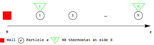
Figure 1: Scheme of the open chain model (see text).

The model consists of $N$ point particles of equal masses $M$ in one dimension arranged on a horizontal line, as sketched in Fig. 1. The particles interact solely with their nearest neighbors through the Lennard-Jones (LJ) potential: $U_{LJ}(r)=E_{LJ}[(r/r_{0})^{-12}-2(r/r_{0})^{-6}]$, where $r$ is the bonding distance and $E_{LJ}$ is the minimum of potential well at $r_{0}$. The particles, indexed in the order of increasing coordinate $x_{a}<x_{a+1},\,a=1..N$, obey the following equation of motion:

$$M\ddot{x}_{a}=-\frac{\partial U_{LJ}(x_{a}-x_{a-1})}{\partial x_{a}}-\frac{\partial U_{LJ}(x_{a+1}-x_{a})}{\partial x_{a}}$$ (2)

in the chain bulk.

The right-most particle (i.e. the last one from the origin, $a=N$) is in contact with a deterministic thermostat that operates according to the Nose-Hoover (NH) scheme at the target kinetic temperature $T$ (Ref. [5]). That is, the equation of motion for the last particle together with the evolution of the thermostatting variable $\chi_{R}$ comprise:

$$M\ddot{x}_{N} =-\frac{\partial U_{LJ}(x_{N}-x_{N-1})}{\partial x_{N}}-\chi_{R}M\dot{x}_{N}$$ (3)

$$\dot{\chi}_{R} =(K_{N}-\frac{1}{2}k_{B}T)/Q$$ (4)

where $K_{N}=M\dot{x}_{N}^{2}/2$ is the kinetic energy of the particle and $k_{B}$ is the Boltzmann constant; $Q$ is an adjustable parameter of thermostat with the characteristic time $\theta=\sqrt{2Q/(k_{B}T)}$.

Analogously, the left-most particle (the first from the origin, $a=1$) is coupled with another NH thermostat. However, we explore two settings of the boundary conditions at the left end. We refer to the open chain, when the first particle interacts by the same Lennard-Jones potential also with a fixed wall placed at the origin point on the left side. The corresponding equations are:

$$M\ddot{x}_{1} =-\frac{\partial U_{LJ}(x_{1})}{\partial x_{1}}-\frac{\partial U_{LJ}(x_{2}-x_{1})}{\partial x_{1}}-\chi_{L}M\dot{x}_{1}$$ (5)

$$\dot{\chi}_{L} =(K_{1}-\frac{1}{2}k_{B}T)/Q$$ (6)

We call the chain free, when the wall on the left side is removed. Then the equation of motion for the first particle reduces to:

$$M\ddot{x}_{1}=-\frac{\partial U_{LJ}(x_{2}-x_{1})}{\partial x_{1}}-\chi_{L}M\dot{x}_{1}$$ (7)

Differently from Ref. [2], there are 2 heat baths in our model, each acting on a single particle. Nonetheless we verified that our results agree with the global NH thermostat. In our computer experiments the case of 2 heat baths converged more quickly to the desired steady state. Furthermore, such setup is rather interesting, for it permits to expose the chain to temperature differences between the thermostats. Therefore to avoid repeating the same statements for both cases, our simulations with the global NH thermostat are not regarded onwards.

The molecular dynamics simulations of the model were performed using the classical Runge-Kutta integrator of 4th order with a time step $\Delta t$ (e.g. Ref. [4]). The programming code ensured that the order of particles relative position was preserved, i.e. $x_{a}<x_{a+1}$, terminating the execution otherwise. The basic units of measure, internally adopted in the computer experiments, were the mass $M$, the length $r_{0}$, and the unit of simulation time $\tau$. The derived unit of energy employed further in the text is defined as $\epsilon=Mr_{0}^{2}/\tau^{2}$. The cartesian coordinates and velocities of particles were sampled each time after $10^{5}$ steps of integration to render $10^{4}$ snapshots of the phase space.

Tbl. 1 introduces numerical parameters common to all the simulations. Note the dimensionless definition of Boltzmann constant implying that the temperature is reported in the units of energy and coincides numerically with the target average kinetic energy of particles.

3 Results

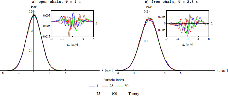
Figure 2: Velocity distributions: kernel density estimations for selected particles from simulations vs. the theoretical curve; the insets depict the deviation $\Delta=\mathrm{Hist}_{a}-\mathrm{PDF}[\dot{x}]$ of a smooth histogram $\mathrm{Hist}_{a}$ from the theory.

Assumed the system represents the canonical ensemble, the velocity $\dot{x}_{a}$ of each $a$-th particle is expected to be distributed normally over a sufficiently long time of simulation. Some smooth histograms constructed from our simulation data by the kernel density estimation method (Ref. [7]) are adduced in Fig. 2: the theoretical curve corresponds to the Probability Density Function (PDF) $\mathrm{PDF}[\dot{x}]\propto\exp(-\frac{K_{a}}{k_{B}T})$. The accurate coincidence of the predicted curve with the computational experiment confirms that the chain is in the state of desired properties.

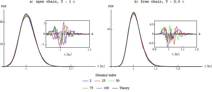
Figure 3: Distance distributions: kernel density estimations for selected bonding distances from simulations vs. the theoretical curve; the insets depict the deviation $\Delta=\mathrm{Hist}_{a}-\mathrm{PDF}[r]$ of a smooth histogram $\mathrm{Hist}_{a}$ from the theory.

As anticipated in the introduction, the distances between particles $r_{a}=x_{a}-x_{a-1},\,a=2..N$ (in the case of the open chain $r_{1}=x_{1}$) can be considered as the configurational degrees of freedom. Their statistical distribution over snapshots are illustrated in Fig. 3 by the smooth histograms alongside the theoretical curve, which is the principle result of the present article and is discussed in the following.

To construct the analytical expression for the distribution of bonding distances, we notice that the smooth histograms are bell-shaped curve centered around $r_{0}$ with the positive skewness. Thus as the first step we pose generically a Gaussian function $\mathrm{PDF}[r]\propto\exp(-\frac{W(r)}{2\sigma^{2}})$. As long as $W(r)$ is a quadratic polynomial of $r$, the very same expression describes the Normal distribution. The skewness accounts essentially for the thermal expansivity, causing the average value to shift from the peak of distribution. It can be controlled by an asymmetric form of $W(r)$.

The asymmetry of interaction potential plays a major role in the thermal expansion. E.g. the pure harmonic interaction, that corresponds to a quadratic polynomial, fails to describe realistically the phenomenon. Perhaps a straightforward way to reproduce this feature through the skewness of expression being derived is to put $W(r)=U_{LJ}(r)$. Next, the denominator under the exponent should have units of energy to respect the dimensionless nature of fraction. By the analogy with the distribution of velocities we take $2\sigma^{2}=k_{B}T$ to obtain:

$$\mathrm{PDF}[r]\propto p(r)=\exp(-\frac{U_{LJ}(r)}{k_{B}T})$$ (8)

Finally, the expression should be normalized to find the coefficient of proportionality $c_{r}$, say. However the integral of the formula built so far doesn’t converge on the support $r\in(0,\infty)$. This difficulty can be treated in various ways, some of which are discussed in the next section. Here to circumvent the problem we introduce a cutoff of the support $r\in(0,2r_{0}]$. It is to note that no cutoff distance was imposed on the interactions in the simulation model.

Indeed one can see from Fig. 3, that PDF drops down to zero very rapidly and practically vanishes outside the range $0.9r_{0}\leq r\leq 1.1r_{0}$. Therefore the suggested support is more than sufficiently representative and may be chosen even narrower. After the normalization on the interval $0\leq r\leq 2r_{0}$, the final formula is obtained:

$$\mathrm{PDF}[r]=\begin{cases}c_{r}\exp(-\frac{U_{LJ}(r)}{k_{B}T}),&\text{if }0\leq r\leq 2r_{0}\\ 0,&\text{if }r>2r_{0}\end{cases}$$ (9)

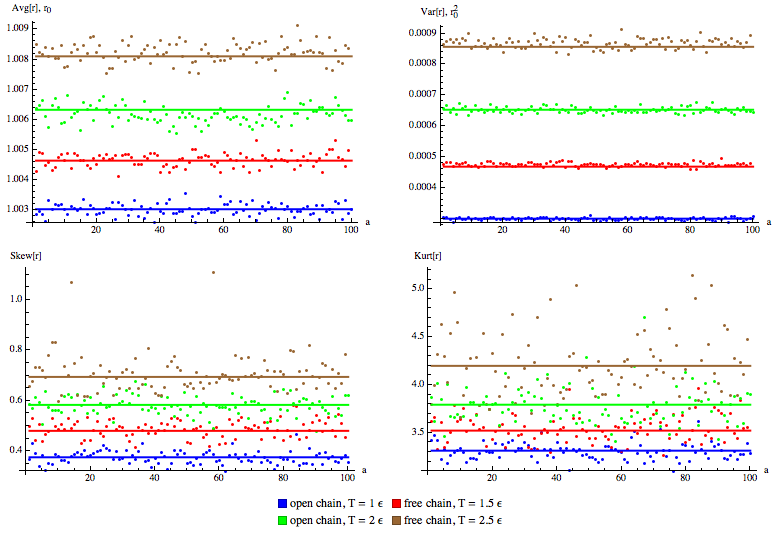
Figure 4: Statistics on inter-particle distances along the chain: theoretical prediction (solid lines) and the estimations from selected simulations (points); $a$ is the index of distance.

Upon the numerical evaluation of integrals required to normalize Eq. 9 at the proper temperatures, the theoretical curves were built in Fig. 3. The expression turns out to describe very accurately at least first 4 moments of the distribution, namely: the average value $\mathrm{Avg}[r]$, the variance $\mathrm{Var}[r]$, the skewness $\mathrm{Skew}[r]$ and the kurtosis $\mathrm{Kurt}[r]$. Fig. 4 compares the theoretical moments with the statistics from the simulations for each particle along. Moreover, they actually appeared almost insensitive to the chosen support on a broad range of the cutoff values. To enforce the argument, we adduce the numeric results in Tbl. 2, where the discrepancy is seen within the second or third significant digit between the theoretical values and the simulation statistics. For excessive lengths of the support notable deviations begin to emerge from the higher orders to the lowers. This effect is more evident at elevated temperatures, as shown in Tbl. 2.

4 Discussions

At first we discuss the alternative procedures to tackle the normalization of $p(r)$. The problem arises due to the limit $\underset{r\to\infty}{\lim}p(r)=1$, which makes the integral $\int_{0}^{\infty}\mathrm{d}rp(r)$ to diverge. A quite efficient solution we elaborated is to expand $U_{LJ}(r)$ in Taylor series around its minimum at $r_{0}$ up to an even power:

$$U_{LJ}(r)=c_{0}+c_{2}(r-r_{0})^{2}+\dots+c_{\alpha}(r-r_{0})^{\alpha}+\mathrm{O}(r^{\alpha+1})=U_{\alpha}(r)+\mathrm{O}(r^{\alpha+1})$$ (10)

where $\alpha$ is even. By the substitution of the truncated form $U_{\alpha}$ in place of $U_{LJ}$, one can recover the normalization on the support $r\in(0,\infty)$.

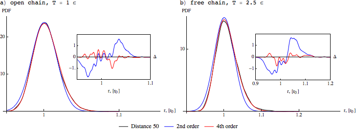
Figure 5: Distributions derived from the truncated expansions of the Lennard-Jones potential in power series around $r_{0}$; the insets depict the deviation $\Delta=\mathrm{Hist}_{50}-\mathrm{PDF}_{n}[r]$ of the smooth histogram $\mathrm{Hist}_{50}$ from the theoretical curve of order $n$.

Obviously, the second order expansion yields a Gaussian, which doesn’t describe appropriately the asymmetry of distribution tails. However, the truncation to power 4 (or greater) suffices to render a good agreement with the simulations. Fig. 5 depicts the just stated by comparison of the PDF curves. The curve of Eq. 9 is not reproduced on the plot, because PDF derived from the 4th order expansion would overlay with it, as well as with the ones procured from truncations to the higher powers.

Another efficient way of normalization on the unbound interval stemmed from an idea to form a product $p(r)f(r)$ with a factor $f(r)$ that tends to 0 at the infinite distance and thus cuts the diverging tail of original distribution. The function $f(r)=\exp\{-\frac{c_{f}(r-r_{0})^{2}}{k_{B}T}\}$ with a constant $c_{f}\leq\epsilon/r_{0}$ having the dimension of energy proved to work fine. We do not have a more specific prescription to choose the value of constant, as the sensitivity of results on $c_{f}$ is really very faint. Although the method certainly fails for $c_{f}\gg\epsilon$, it is difficult to propose any reasonably optimal recommendation, but to set it as small as possible.

The mechanism of the last method can be understood by considering again the expansion Eq. 10:

$$p(r)f(r)=\exp\{-\frac{c_{0}+(c_{1}+c_{f})(r-r_{0})^{2}+\mathrm{O}(r^{3})}{k_{B}T}\}$$ (11)

Thus the factor introduces a correction into the second order term of expansion, causing the power series to diverge and the exponent to vanish at $r\to\infty$. The original distribution is recovered for $c_{f}\to 0$.

By construction, the suggested normalizations are rather convenient approximations. Both methods produce good numerical predictions on statistics observed in simulations. Nonetheless Eq. 9 perhaps seems more fundamental. Indeed, one should account that as an artifact of low dimensionality the free and open chains with Lennard-Jones interactions may get broken sometimes during the simulation. In such cases, the broken pieces of chain can stand for long times at distances $r\gg 2r_{0}$. Consequently, one would find an outcast statistics and the distribution Eq. 9 would fail. Discarding these cases, the chain is implicitly assumed to stay bound, i.e. with particles within certain limits of separation distances.

On the contrary, when the larger distances are admitted in the support, the normalization constant $c_{r}$ tends to zero as the integral of $p(r)$ diverges. In that limit, distances of arbitrary values become equally probable coherently with the possibility of chain to break. In fact, the bound state we adopt to model a solid in the equilibrium can be viewed as a metastable state of our FPU-like chain, which is characterized by the Gaussian distribution of velocities and Eq. 9.

The bonding distances corresponds to the one-dimensional analogue of the so called internal coordinates. Once their distribution is known, statistics for the configurational degrees of freedom in alternative reference frames should be in principle derivable. E.g., in the open chain the Cartesian coordinate of $a$-th particle, say, is $x_{a}=\sum_{b=1}^{a}r_{a}$. Then it could be regarded as a sum of $a$ random variables. It follows though, that the distribution of Cartesian coordinates would vary by parameters from particle to particle. For this reason the consideration of distances occasionally is simpler, since they are directly related to the potential energy. In systems of the higher dimensionality, the internal coordinates would comprise also the angles. Therefore the generalization is not so straightforward.

5 Conclusion

The presented theoretical developments do not constitute a de principio mathematical derivation for the final expression. Nonetheless the stated heuristic formulation is strikingly supported by the computational approach with both numerical and qualitative arguments.

The distribution is valid for the bound state of the FPU-chain with realistic potentials, which models a solid in equilibrium with heat baths at its boundaries. The expression degrades consistently to zero, when the chain is allowed to break and to expand in space arbitrarily.

The statistics of bonding distances is central to many important characteristics of solids. The distributions themselves are fundamental for account of thermal vibrations in X-Ray analysis of the atomic structure. Their average values represent the equilibrium bond lengths. Finally, the distribution of their sum determines the thermal expansion. The assessment of the analytical form inspires much interest as the means to analyze and calculate immediately such properties.

Parameter	Value
Number of particles, $N$	100
Depth of potential, $E_{LJ}$	$100\,\epsilon$
Boltzmann constant, $k_{B}$	$2$
Thermostat constant, $Q$	$10\,Mr_{0}^{2}$
Integration time step, $\Delta t$	$10^{-4}\,\tau$
Total time of simulation	$10^{5}\,\tau$

Table 1: Numerical parameters of simulations

	Distances $r_{a}$			Theory on various supports
Statistics	25	50	100	$(0,1.2]$	$(0,2]$	$(0,10^{2}]$	$(0,10^{3}]$
Open chain, $T=1\,\epsilon$
$\mathrm{Avg}[r]\text{, }r_{0}$	1.00326	1.00278	1.00303	1.00303	1.00303	1.00303	1.00303
$\mathrm{Var}[r]\text{, }10^{-3}\cdot r_{0}^{2}$	0.298683	0.297016	0.305084	0.299494	0.299494	0.299494	0.299495
$\mathrm{Skew}[r]$	0.411562	0.349918	0.355817	0.376281	0.376281	0.3765	2.5735
$\mathrm{Kurt}[r]$	3.39459	3.24474	3.27969	3.31398	3.31398	13.4244	1.0 $\cdot 10^{6}$
Free chain, $T=2.5\,\epsilon$
$\mathrm{Avg}[r]\text{, }r_{0}$	1.00770	1.00756	1.00836	1.00810	1.00811	1.02316	2.51529
$\mathrm{Var}[r]\text{, }10^{-3}\cdot r_{0}^{2}$	0.854042	0.840263	0.893070	0.854428	0.856988	10022.9	1.0 $\cdot 10^{7}$
$\mathrm{Skew}[r]$	0.668215	0.666151	0.784553	0.674415	0.694886	236.632	74.7975
$\mathrm{Kurt}[r]$	3.98040	4.18547	4.47063	4.00426	4.19941	59733.9	5968.99

Table 2: Numerical comparison of statistics: selected distances from simulations and the theoretical predictions based on various cutoffs of the support.

References

- [1] Livia Conti, Paolo De Gregorio, Michele Bonaldi, Antonio Borrielli, Michele Crivellari, Gagik Karapetyan, Charles Poli, Enrico Serra, Ram-Krishna Thakur, and Lamberto Rondoni. Elasticity of mechanical oscillators in nonequilibrium steady states: Experimental, numerical, and theoretical results. Physical Review E, 85, 2012.
- [2] Paolo De Gregorio, Lamberto Rondoni, Michele Bonaldi, and Livia Conti. One-dimensional models and thermomechanical properties of solids. Physical Review B, 84, 2011.
- [3] Giovanni Gallavotti, editor. The Fermi-Pasta-Ulam Problem. Springer, 2008.
- [4] Ernst Hairer, Syvert P Nørsett, and Gerhard Wanner. Solving ordinary differential equations I. Springer, 2nd edition, 2008.
- [5] Owen G Jepps and Lamberto Rondoni. Deterministic thermostats, theories of nonequilibrium systems and parallels with the ergodic condition. Journal of Physics A: Mathematical and Theoretical, 43, 2010.
- [6] James P Sethna. Statistical mechanics: Entropy, Order Parameters and Complexity. Oxford University Press, 2006.
- [7] B W Silverman. Density Estimation for Statistics and Data Analysis. Chapman and Hall / CRC Press LLC, London, New York, 2000.