Direct model fitting to combine dithered ACS images

The information lost in images of undersampled CCD cameras can be recovered with the technique of ‘dithering’. A number of subexposures is taken with sub-pixel shifts in order to record structures on scales smaller than a pixel. The standard method to combine such exposures, ‘Drizzle’, averages after reversing the displacements, including rotations and distortions. More sophisticated methods are available to produce, e.g., Nyquist sampled representations of band-limited inputs. While the combined images produced by these methods can be of high quality, their use as input for forward-modelling techniques in gravitational lensing is still not optimal, because the residual artefacts still affect the modelling results in unpredictable ways. In this paper we argue for an overall modelling approach that takes into account the dithering and the lensing without the intermediate product of a combined image. As one building block we introduce an alternative approach to combine dithered images by direct model fitting with a least-squares approach including a regularization constraint. We present tests with simulated and real data that show the quality of the results. The additional effects of gravitational lensing and the convolution with an instrumental point spread function can be included in a natural way, avoiding the possible systematic errors of previous procedures.

1 Introduction

The light distribution detected by a CCD in an astronomical observation does not resemble the brightness distribution on the sky exactly but is affected by the properties of the optical instrument. The most important effect is the point-spread-function (PSF). If we neglect small variations of PSF with position, it can be described as a convolution of the true light distribution. The effect is caused by diffraction in the instrument and, for ground-based telescopes, by the atmospheric ‘seeing’.

In addition, the design of the instrument can cause a geometric distortion. In the case of the Advanced Camera for Surveys (ACS) of the Hubble Space Telescope (HST), the off-axis location of the detectors (tilted focal surface with respect to the light rays) and the Optical Telescope Assembly (OTA) cause anisotropic variations in the plate scale. The first ACS geometric distortion campaign observed the core of 47 Tucanae with the WFC (Wide Field Channel) and HRC (High Resolution Channel). A fit of a 4th order polynomial corrects the distortion to an accuracy of 0.1–0.2 pixels over the entire field of view (Clamping et al. 2000).

Each pixel integrates the light over its area (and slightly beyond) weighted with the ‘pixel response function’, assumed to be the same for all pixels. This can mathematically be described as a convolution with this response function and subsequent multiplication with a ‘bed-of-nails’ sampling function.

Therefore if we consider the true light distribution as $I^{*}$, we can write the observed light distribution as

$$I^{\textrm{obs}}=S\cdot R\star D\otimes P\star I^{*}.$$ (1)

Here $P$ represents the PSF, $D$ the effect of optical distortion, $R$ the response function and $S$ the sampling function. A convolution is denoted by $\star$, an arbitrary mapping by $\otimes$ and a multiplication by a dot. For our image analysis we either have to ‘invert’ this process, by trying to construct a realistic representation, e.g. band-limited, of the input image, or take it into account in a modelling process.

In order to reveal information on scales smaller than the pixel size, observations are ‘dithered’, i.e. split into several exposures that are shifted relative to each other by sub-pixel displacements. Inverting the convolution with $P$ requires the conservation of structures on scales smaller than the PSF width; the sampling must be sufficiently fine to resolve the PSF. For ground-based telescopes, $P$ is dominated by the atmospheric seeing, and modern CCD instruments generally have sufficient resolution. For the WFC of ACS, the pixel size of 0.05 arcseconds is comparable to the overall PSF width, and dithering is essential to recover any of the fine-scale structure of the PSF.

1.1 Image combination and lens modelling

There are a number of known methods that can invert (in the sense described above) the measurement process and produce an estimate of the true light distribution under certain assumptions for its properties (see below). Our main interest are gravitational lenses, and here the main goal is not a good estimate of the true (gravitationally lensed) sky brightness distribution. Instead we want to derive good models for the unlensed brightness distribution of the source and in particular good models for the mass distribution that causes the lensing effect.

Sophisticated methods are available that can invert the effect of the lens mapping in order to reconstruct the unlensed source and to determine the mass distribution of the lens (e.g. Jullo et al. 2007; Suyu et al. 2006; Warren & Dye 2003). However, they all rely on an accurate input image that is free of systematic artefacts. Because of the complexity of the overall problem, the effect of artefacts in the input image on the final result are not easy to judge. Even the best reconstruction methods will necessarily introduce errors into the reconstructed $I^{*}$, and the optimal way of doing the lens modelling is not to first make an optimal image and then use that as basis for the mass models of the lens. Instead we eventually want to combine both parts and include the lens effect as part of the measurement process and fit for the true brightness distribution of the source and the mass model of the lens, without the intermediate result of a combined image. Even though the final reconstructed image of the unlensed source will still suffer from minor systematic effects, the effect on the mass models will be less severe and much better understood.

In the notation of Eq. (1) the lens acts as another generally complicated mapping of the unlensed brightness distribution to form $I^{*}$. This mapping is linear in the brightness distribution but depends non-linearly on the lens model parameters. The final algorithm will thus consist of two nested parts, where the inner one determines the best brightness distribution of the source for a given lens model, while the outer one will vary the lens model itself to minimize the residuals.

This paper describes the first step in this direction, consisting of an algorithm that solves parts of Eq. (1) by explicitly modelling the optimal true brightness distribution that fits the data, taking into account the dithering with full correction for distortion, and at the same time obeys the necessary regularization constraints.

Some of the image combination methods described below reconstruct a Nyquist sampled representation of the observed sky brightness distribution that has to be band-limited as result of the finite instrumental aperture. Such an approach is not appropriate in our case, because the lens mapping will destroy this property for the brightness distribution of the source. Instead we employ a smoothness regularization constraint.

We emphasize that out modelling algorithm is not meant to replace other methods to produce combined images, but to provide a major part of a full algorithm that will include the action of the lens and the convolution with the PSF. As test of this part we nevertheless use the combined images as a demonstration.

1.2 Known image combination methods

A basic method to combine these dithered images is a linear technique, ‘shift-and-add’. In this method, pixels of each image are transferred to a finer grid, shifted to the same position and added to the output image. In the formalism introduced above this corresponds to a convolution with another function $R^{\prime}$ that represents the size and shape of the pixels. Neglecting the distortion for the moment, and assuming a uniform and complete dithering pattern (so that the sampling $S$ can be neglected), the result would correspond to $R^{\prime}\star R\star P\star I^{*}$. This additional convolution with the pixel size reduces the resolution of the result. The geometric distortion is generally not taken into account in this simple process.

‘Drizzle’, the standard method to combine dithered HST images, extends this approach by allowing for arbitrary shifts and rotations, by correcting for the distortion and by using more sophisticated techniques to transfer the images to finer grids. The general approach, however, is based on shift-and-add, and Drizzle always introduces a convolution function $R^{\prime}$ (Fruchter & Hook 2002).

Drizzle adds small high-frequency artefacts to the image (Figure 1 in Fruchter (2011) shows this effect) which is detrimental in cases where preservation of the true PSF is needed. On larger scales (larger than the original pixels) these artefacts are averaged out. More details are provided in Fruchter (2011).

With nearly interlaced dithered images, high-fidelity combined images can be created with the method introduced by Lauer (1999). This method attempts to predict the values of the output image based on dithered data but it can not handle image distortions. It is based in the Fourier transform of the images. The final image is computed as a linear combination of the transformed input images. In this process the aliased components are removed algebraically.

Rowe et al. (2011) present a method (Imcom) to combine undersampled images for band-limited data. Imcom is developed to process data based on linear algorithm approach in Fourier space. In this method, the assumed function for the PSF (including jitter, optics of the instrument and the response of the CCD) is specified for each pixel of the images. The required information to derive the function comes from the optical model for the instrument and/or stars in the field. The fully parametric model can be adopted for this PSF function.

Fruchter (2011) introduce the (iDrizzle) method, which is based on Drizzle but removes high frequency artefacts using the assumption of a band-limited image. The iterative Drizzle approach also eliminates the convolution with an additional kernel that is inherent in Drizzle.

The available methods have in common that they are designed to produce a combined image without direct forward modelling. They are thus not easily useable as part of the full lens modelling process.

2 The direct fitting method

The development of an alternative combining method was prompted by the case of the gravitational lens system B0218+357 (Patnaik et al. 1992). With 334 mas it has the smallest image separation of all known galaxy-scale lenses, and very accurate positions of the images relative to the lensing galaxy are required for a reliable determination of the Hubble constant from the time delay (Biggs et al. 1999). York et al. (2005) used Drizzle to combine the data to determine the position of the galaxy relative to the lensed images from deep ACS observations. They were able to improve the determination of $H_{0}$ in this way, but the accuracy of the result is limited by imaging artefacts and PSF inaccuracies.

Here we introduce an alternative method to combine the observed images. This method is based on fitting a brightness distribution to the observed exposures with a least-squares method. Since we want to overcome the undersampling problem, we use a finer grid for the model image. A smoothness constraint is employed in order to obtain a unique and realistic solution for the final result. Because the resolution in the output image is higher than in the original input images, it is obvious that such an additional constraint is required to avoid unconstrained output pixels.

The model is pixelized in the sky coordinates, and in the transformation between CCD and sky coordinates the geometric distortion correction is taken into account. We use a simplified (currently without explicit convolution with the PSF and pixel-response function) version of the imaging equation (1) to predict the observed brightness distributions in CCD coordinates for a given model. The deviations of these predictions from the real observations are then minimized by varying the model pixel values.

The function that is being minimized can be written as

$$f=\sum_{j=1}^{n_{\rm im}}\sum_{i=1}^{n_{\rm pix}}\frac{\left(I^{\textrm{mod}}_{\textrm{int}(j)}[i]-I^{\textrm{obs}}_{(j)}[i]\right)^{2}}{\sigma_{ij}^{2}}w_{ij}+\lambda R(n)$$ (2)

where ${n_{\rm im}}$ is the total number of images that we want to combine, ${n_{\rm pix}}$ is the number of CCD pixels per image, $I^{\textrm{mod}}$ is the brightness distribution model in sky coordinates, and $I_{(j)}^{\textrm{obs}}$ the observed image $j$. The subscript ‘int$(j)$’ denotes interpolation to the same grid as the observed image $j$, taking into account the distortion, shift and rotation in the conversion between CCD coordinates and sky coordinates. $\sigma_{ij}$ is the uncertainty of pixel $i$ in image $j$. The additional weight function $w_{ij}$ is set to zero for flagged or masked bad or unwanted pixels and to one otherwise. Most important is cosmic ray flagging using the data quality layer of the calibrated and flat fielded data (flt images). The strength of the smoothness constraint is given by the coefficient $\lambda$. More details on choosing this parameter can be found in section 3.

$R(n)$ is a quadratic operator that measures non-smoothness, where $n$ denotes the order of derivatives included. Most commonly used are gradient minimization ($n=1$) and curvature minimization ($n=2$):

$$R(1) = \sum_{i=1}^{n_{\rm modpix}}\left[\left(\frac{\partial I^{\textrm{mod}}}{\partial x}[i]\right)^{2}+\left(\frac{\partial I^{\textrm{mod}}}{\partial y}[i]\right)^{2}\right]$$ (3)

$$R(2) = \sum_{i=1}^{n_{\rm modpix}}\left(\frac{\partial^{2}I^{\textrm{mod}}}{\partial x^{2}}[i]+\frac{\partial^{2}I^{\textrm{mod}}}{\partial y^{2}}[i]\right)^{2}.$$ (4)

Here we are summing over all ${n_{\rm modpix}}$ model pixels which is generally different from ${n_{\rm pix}}$. The derivatives of the discrete model brightness distributions are determined using finite differences.

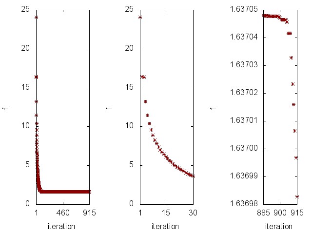
In our work we use $n=1$, but in order to study the effect of smoothing on our model, we also considered the case of $n=2$. The function $f$ is quadratic in the unknown parameters so that the mininization corresponds to solving a system of linear equations. This could in principle be done directly. However, this is not trivial given the size of the system. For a $(1{\rm k})^{2}$ model image, the matrix that has to be inverted has $10^{12}$ elements. Instead we use the more general numerical minimization scheme named after Broyden, Fletcher, Goldfarb & Shanno (BFGS). This quasi-Newtonian algorithm (Press et al. 1992) uses analytical gradients and builds up information on the Hessian matrix iteratively. We use a limited-memory version (L-BFGS) that does not require storage of the full matrix and allows us to process the data on normal desktop computers.

In order to study how the smoothness constraint affects the combined output image, we describe the effect as a convolution. If we assume small pixels (large ${n_{\rm pix}}$ and ${n_{\rm modpix}}$) and $\sigma=1$, we can write Eq. (2) with continuous integrals as

$$f=\iint\left[I^{\textrm{mod}}(x,y)-I^{\textrm{obs}}(x,y)\right]^{2}\,\mathrm{d}x\,\mathrm{d}y+\lambda R(n)$$ (5)

with

$$R(1) = \iint\left[\left(\frac{\partial I^{\textrm{mod}}}{\partial x}\right)^{2}+\left(\frac{\partial I^{\textrm{mod}}}{\partial y}\right)^{2}\right]\mathrm{d}x\,\mathrm{d}y,$$ (6)

$$R(2) = \iint\left(\frac{\partial^{2}I^{\textrm{mod}}}{\partial x^{2}}+\frac{\partial^{2}I^{\textrm{mod}}}{\partial y^{2}}\right)^{2}\mathrm{d}x\,\mathrm{d}y.$$ (7)

This approach is accurate in the limit of fine sampling of $I^{\textrm{mod}}$ and dense dithering patterns. Considering Parseval’s theorem, we can transfer this equation to Fourier space which makes the calculation simpler. This leads to a uniform expression for $n=1,2$,

$$f=\iint\left|\widehat{I^{\textrm{mod}}}(u,v)-\widehat{I^{\textrm{obs}}}(u,v)\right|^{2}\,\mathrm{d}u\,\mathrm{d}v+$$

$$\lambda^{\prime}\iint k^{2n}\left|\widehat{I^{\textrm{mod}}}(u,v)\right|^{2}\,\mathrm{d}u\,\mathrm{d}v,$$ (8)

where $k^{2}=u^{2}+v^{2}$ and $\lambda^{\prime}=(2\pi)^{2n}\lambda$. Minimizing $f$ requires that the integrand is minimized, which results in

$$\widehat{I^{\textrm{mod}}}(u,v)=\frac{\widehat{I^{\textrm{obs}}}(u,v)}{1+\lambda^{\prime}k^{2n}}.$$ (9)

From Fourier theory we know that the multiplication of two functions in Fourier space corresponds to the convolution of those functions in image space. We can determine this convolution function $C(x,y)$ from the inverse transform of $1/(1+\lambda k^{2n})$

$$C(x,y)=\iint\frac{1}{1+\lambda^{\prime}k^{2n}}\mathrm{e}^{2i\pi\@vec{k}\cdot\@vec{x}}\,\mathrm{d}u\,\mathrm{d}v\,,\,\@vec{k}=(u,v).$$ (10)

In the following we study this inverse transform for $n=1$ and $n=2$.

Gradient minimization, $n=1$:

We invert the Fourier transform in spherical coordinate with $(x,y)=r(\cos\phi,\sin\phi)$ and $(u,v)=k(\cos\theta,\sin\theta)$.

$$C(r) = \frac{1}{\lambda^{\prime}}\int\limits_{0}^{\infty}\int\limits_{0}^{2\pi}\frac{k}{\frac{1}{\lambda^{\prime}}+k^{2}}\mathrm{e}^{2i\pi kr\cos(\theta-\phi)}\,\mathrm{d}k\,\mathrm{d}\theta$$ (11)

$$= \frac{2\pi}{\lambda^{\prime}}\int\limits_{0}^{\infty}\frac{k}{\frac{1}{\lambda^{\prime}}+k^{2}}\mathrm{J}_{0}(2\pi kr)\,\mathrm{d}k$$ (12)

This integral is the definition of the Hankel transform of $(1/\lambda^{\prime}+k^{2})^{-1}$, which leads us to

$$C(r)=\frac{2\pi}{\lambda^{\prime}}\mathrm{H}\left\{\frac{1}{\frac{1}{\lambda^{\prime}}+k^{2}}\right\}.$$ (13)

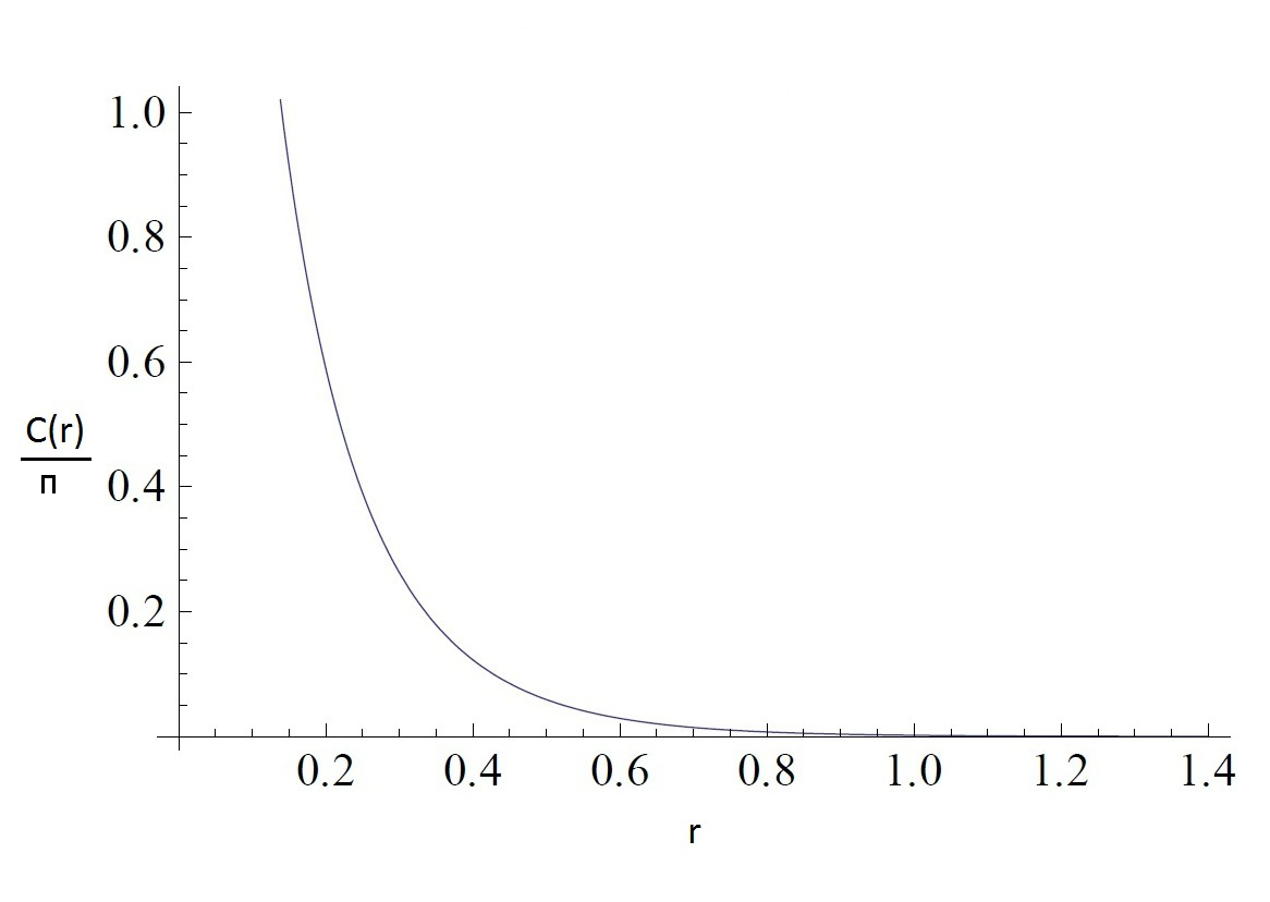
The Hankel transform of this function is the modified Bessel function of the second kind (Piessens 2000). Hence the convolution function becomes

$$C(r)=\frac{2\pi}{\lambda^{\prime}}\mathrm{K}_{0}\left(\frac{2\pi r}{\sqrt{\lambda^{\prime}}}\right).$$ (14)

The behaviour of this convolution function is shown in Figure 1.

Figure 1: Convolution function $C(r)$ for gradient minimization ($n=1$) with $\lambda^{\prime}=1$. The singularity at the origin is logarithmic.

Curvature minimization, $n=2$:

For this case, the convolution function becomes

$$C(r)=\frac{2\pi}{\lambda^{\prime}}\mathrm{H}\left\{\frac{1}{\frac{1}{\lambda^{\prime}}+k^{4}}\right\}.$$ (15)

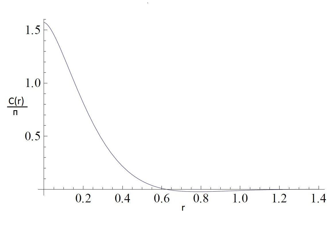
This results in the Kelvin function $\mathrm{Kei}_{0}$ (Piessens 2000):

$$C(r)=\frac{-2\pi}{\sqrt{\lambda^{\prime}}}\mathrm{Kei}_{0}\left(\frac{2\pi r}{\sqrt[4]{\lambda^{\prime}}}\right)$$ (16)

Figure 2 presents the behaviour of this convolution function.

Figure 2: Convolution function $C(r)$ for curvature minimization ($n=2$) with $\lambda^{\prime}=1$. In contrast to the case of $n=1$ this function is regular at the origin.

3 Tests of the direct fitting method

In our current implementation the algorithm consists of two separate parts. A Python script is used to calculate the mapping between CCD pixels and sky coordinates using the geometric distortions with parameters derived from the available meta-data. Particularly between different HST ‘visits’, the dither offsets from the FITS headers are generally not sufficiently accurate. In this case they have to be determined using cross-correlation techniques or by using the positions of reference stars. In the results presented here, this was not necessary. Information about the mapping is added to the FITS images which are then read by the main minimization program written in C. For the minimization we use the GSL (GNU Science Library) variant of L-BFGS.

In this section we present the combined images of simulated and real data based on our method. As real data we use observations of the two gravitational lensing systems B1608+656 and B0218+357.

Simulated Data

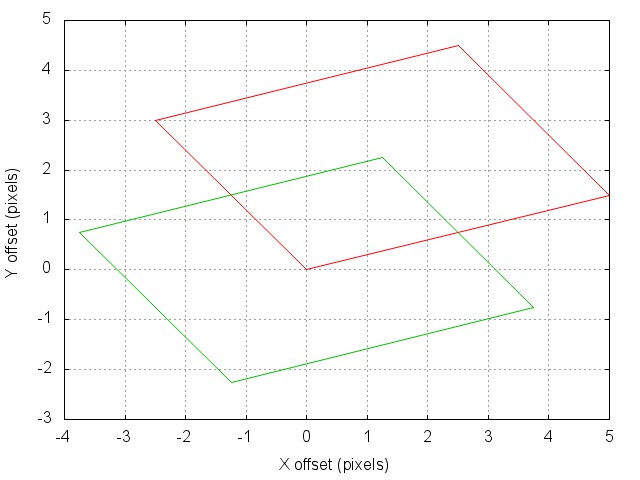
For the simulated data, we produced 20 images (a dithering pattern of the ACS as shown in figure 3 was used in the simulation) consisting of two sources with Gaussian brightness distributions at fixed separation. This setup was chosen to roughly resemble the case of B0218+357 in which relative positions are the most important parameter. Realistic Poisson noise was added to the simulated images.

Figure 3: Box dither pattern used for the simulated data and real data.

The simulated images were combined with our method using a model pixel size of 30 mas. We then used galfit (Peng et al. 2010) to fit the source parameters as a test of the reconstruction accuracy. To study the effects of a varying smoothing coefficient we used these simulated data and combined them with different $\lambda$ (Fig. 4).

Figure 4: Top: Fitting results for the simulated images using smoothing coefficients of $\lambda=10^{-1}$, $10^{-3}$ and $10^{-5}$. Bottom: Corresponding residuals relative to the input image.

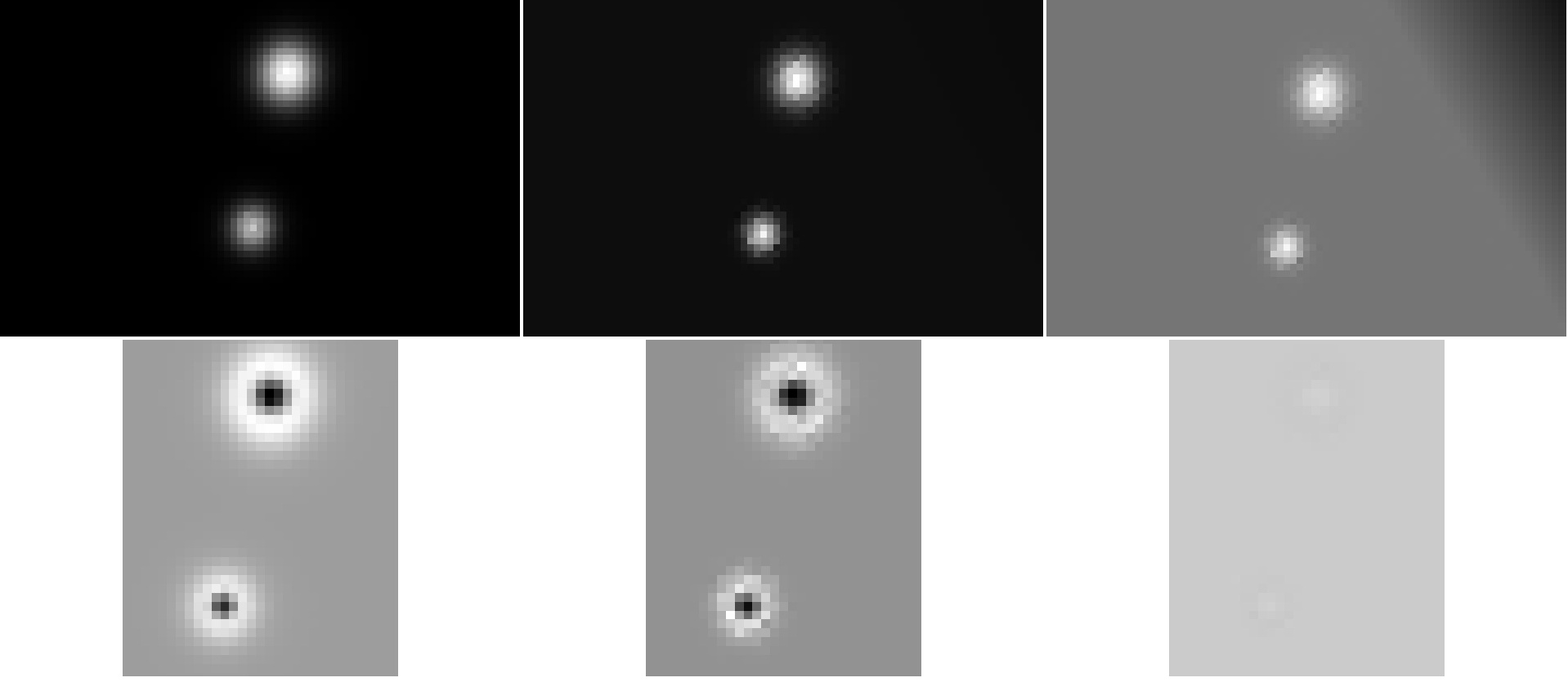
Table 1 presents the fitted separation of the sources in the combined image for different values of $\lambda$.

Table 1: Comparison between the true separation of 0.72358 and the separation determined by galfit.

$\lambda$	separation [arcsec]	error of separation [arcsec]
$10^{-1}$	0.7268	0.0032
$10^{-2}$	0.7260	0.0025
$10^{-3}$	0.7257	0.0022
$10^{-4}$	0.7251	0.0015
$10^{-5}$	0.7238	0.0002

As can be seen from the table, $\lambda=10^{-5}$ provides the best determination of the distance between the two simulated sources. For real observations, the coefficient $\lambda$ can be determined by comparing the $\chi^{2}$ of the fits for different values of $\lambda$ and selecting the one that is closest to the statistical expectation.

We conclude that the direct fitting approach can produce combined images that in principle allow relative position measurements with an accuracy well beyond 1mas.

B1608+656

As a first test of the method on real data, we used the strong lensing system B1608+656. We chose an observation consisting of 44 images observed in the F814W filter with the ACS/WFC.

We applied the direct fitting method with different smoothing coefficients and pixel sizes to find the optimal $\lambda$ for these data. Figure 5 shows the variation of $\chi^{2}$ as a function of $\lambda$ for different pixel sizes.

Figure 5: Reduced $\chi^{2}$ as a function of $\lambda$ for B1608+656. Different colours and symbols represent pixel sizes from 10 to 30 mas.

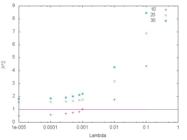
For a pixel size of 10 mas we find that $\lambda=10^{-3}$ results in a reduced $\chi^{2}$ of 1.029, very close to the expected 1. Generally smaller values for $\lambda$ produce a better fit, as expected. However, for pixel sizes of 20 and 30 mas, $\chi^{2}$ never drops below unity. In these cases the large pixels themselves serve as additional regularization that is too strong to achieve a reduced $\chi^{2}$ of unity.

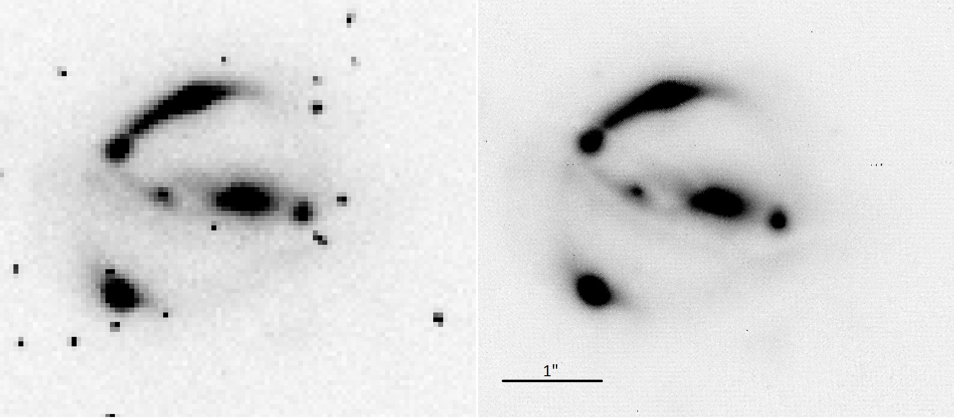
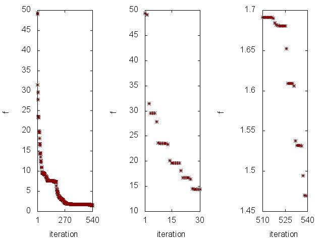
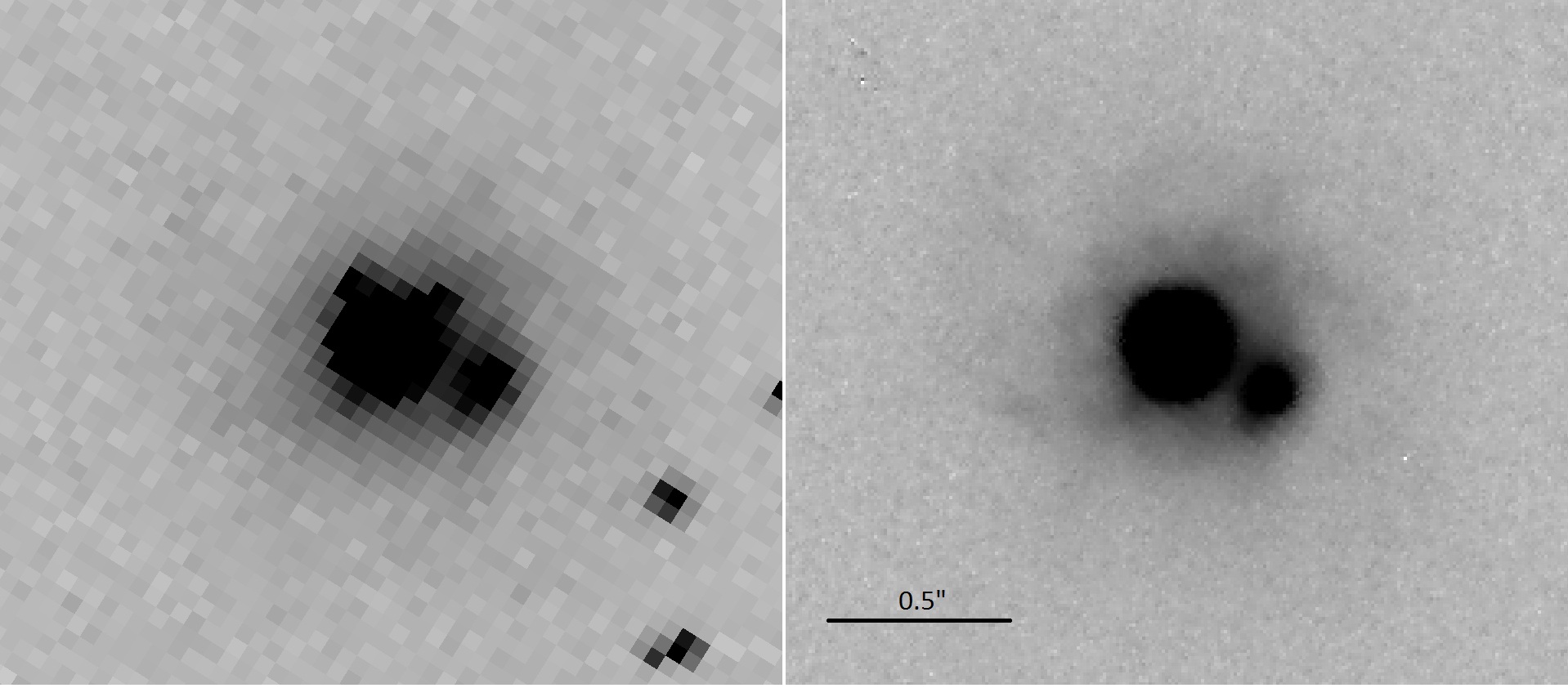
Figure 6 shows one of the raw images and the combined image using a pixel size of 10 mas and the optimal $\lambda=10^{-3}$.

Figure 6: Top: One of the raw images of B1608+656 and combined image using the direct fitting method with $\lambda=10^{-3}$ and pixels of 10 mas. Bottom: Progress of the minimization of $f$ for all iterations, for the first iterations and for the final iterations. The final reduced $\chi^{2}$ for the combined image is $1.029$.

B0218+357

A second test was performed for the system B0218+357 that provided our main motivation for the development of the fitting method.

Of the observations described by York et al. (2005) we restricted ourselves to visit 13, containing 20 images taken with ACS/WFC and the F814W filter. In order to determine the best $\lambda$ we used the same procedure as for B1608+656 and plotted the resulting $\chi^{2}$ for a range of $\lambda$ and pixel sizes (Fig. 7). We find that $\lambda=10^{-3}$ with $\chi^{2}=1.008$ is close to the optimum. A pixel size of 30 mas is again too large for a good fit, but 20 mas would just be sufficient for a smaller $\lambda$.

Figure 7: Reduced $\chi^{2}$ as function of $\lambda$ for B0218+357. Different colours and symbols represent pixel sizes from 10 to 30 mas.

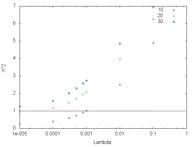
Figure 8 shows the combined image resulting from the direct fitting method with a pixel size of 10 mas.

Figure 8: Top: One of the raw images of B0218+357 and combined image using a pixels size of 10 mas and $\lambda=10^{-3}$. Bottom: Progress of the minimization of $f$ for all iterations, for the first iterations and for the final iterations.

4 Conclusions and outlook

In observations with undersampling cameras, many exposures with sub-pixel shifts (dithering) are usually taken to record information on scales smaller than a pixel. Drizzle and more sophisticated methods can be used to recover this information and produce combined images of high quality. However, even the best methods cannot avoid artefacts in the combined images, implying that such images are not well suited as input for further model fitting, e.g. in the case of gravitational lenses where the true (unlensed) brightness distribution of the source as well as the mass distribution causing the lensing are to be determined. In such a situation, a direct model-fitting approach is much more appropriate to tackle this inverse problem.

In this paper we presented a basic building block for such a fitting procedure. Instead of trying to combine the dithered images by shifting and adding, or by constructing a representation that is band-limited and consistent with all input images, we directly fit the true brightness distribution of the sky to the observed images. In this process we correct for the geometric distortion and take possible flagging into account. A smoothness constraint is added to allow for a unique solution and to avoid unrealistic small-scale fluctuations and noise amplification. This approach of direct model fitting has the advantage that the additional mapping caused by a gravitational lens can later be included easily.

Tests with real and simulated data show that the fitting method works well and produces accurate results. In the future we will use combined images of B0218+357 to determine the relative positions of the lensed images and the lensing galaxy with optimal accuracy. This is an essential input for modelling efforts that are needed to convert the measured time delay into a robust estimate of the Hubble constant. Previous attempts in this direction suffered from the shortcomings of Drizzle and corresponding difficulties in fitting the PSF (York et al. 2005). It is our hope that our alternative combining method can improve these results.

Currently the fitting approach does not include the convolution with the PSF and the pixel response function. These can be included in a natural way so that an extended version will be able to ‘invert’ these effects as well. Additionally, the effect of a gravitational lens also acts linearly on the brightness distribution, which allows for its inclusion in the same formalism. With such an overall algorithm, we will be able to fit the unlensed brightness distribution of the source directly. The optimal mass distribution of the lens can then be found by minimizing the remaining residuals. We hope that this approach of a global fit will be much more reliable and robust than the standard process of first combining the images, then deconvolving the PSF and pixel response function with subsequent inversion of the lensing effect. Similar applications are possible in other fields.