Quantum-defect theory for $-1/r^{4}$ type of interactions

Abstract

We present a quantum-defect theory (QDT) for the $-1/r^{4}$ type of long-range potential, as a foundation for a systematic understanding of charge-neutral quantum systems such as ion-atom, ion-molecule, electron-atom, and positron-atom interactions. The theory incorporates both conceptual and mathematical advances since earlier formulations of the theory. It also includes more detailed discussions of the concept of resonance spectrum and its representations, universal properties in charge-neutral quantum systems, and the QDT description of scattering resonances that is applicable to any $-1/r^{n}$ potential with $n>2$.

I Introduction

The quantum-defect theory (QDT) for $-1/r^{4}$ type of interactions, if broadly defined as a quantum theory that explicitly takes advantage of the universality due to the long-range potential, has existed in various forms for decades O’Malley et al. (1961); Watanabe and Greene (1980); Fabrikant (1986). Notably, the theory of O’Malley et al. O’Malley et al. (1961) gives an analytic description of ultracold electron-atom and ion-atom collision that has stood for many years. The theory of Fabrikant Fabrikant (1986) gives a theory of scattering that takes further advantage of the modified Mathieu functions Holzwarth (1973); Khrebtukov (1993); Olver et al. (2010). The theory of Watanabe and Greene Watanabe and Greene (1980) gives a more complete QDT formulation for $-1/r^{4}$ potential in that it treats both positive and negative energies in a consistent QDT manner which is important for, e.g., its application in a multichannel formulation to describe Fano-Feshbach resonances. Together, these theories have provided a solid theoretical backbone for our understanding of charge-neutral quantum systems in low-energy regimes or around a dissociation (detachment) threshold, and have served us well for many years, including in more recent applications such as Rydberg molecules Greene et al. (2000); Bendkowsky et al. (2009, 2010); Löw et al. (2012).

Renewed interest in QDT for $-C_{4}/r^{4}$ polarization potential has arisen with the emergence of cold ion-atom Côté and Dalgarno (2000); Grier et al. (2009); Idziaszek et al. (2009); Gao (2010a); Zipkes et al. (2010a, b); Schmid et al. (2010); Rellergert et al. (2011); Hall et al. (2011); Idziaszek et al. (2011) and ion-molecule interactions and reactions Willitsch et al. (2008); Staanum et al. (2008); Roth et al. (2008); Hudson (2009); Gao (2011a); Willitsch (2012). For such heavier systems, the QDT takes on a different magnitude of importance for three primary reasons. First, a same long-range polarization potential, which in the case of electron-atom interaction can only bind a few states or lead to a few resonances Buckman and Clark (1994), can bind many more states and lead to many more resonances. Their existence implies a rapid energy variation induced by the long-range interaction, making the QDT description far more important and necessary. Mathematically, this greater importance of long-range potential for heavier systems is reflected in the length scale, $\beta_{4}\equiv(2\mu C_{4}/\hbar^{2})^{1/2}$, and the corresponding energy scale, $s_{E}=(\hbar^{2}/2\mu)(1/\beta_{4})^{2}$, associated with a $-C_{4}/r^{4}$ interaction. The length scale $\beta_{4}$ scales with the reduced mass as $\mu^{1/2}$, and is hundreds times greater for ion-atom Gao (2010a) and ion-molecule Gao (2011a) systems than for electron-atom systems. The energy scale $s_{E}$ scales with the reduced mass as $\mu^{-2}$, and is typically $10^{9}$ times smaller Gao (2010a, 2011a). Between a fixed energy $\epsilon$ and the dissociation threshold $\epsilon=0$, the number of bound states or resonances due to the long-range potential is determined by the scaled energy $\epsilon/s_{E}$ (see Ref. Gao (2010a) and Sec. III.2.3), which is vastly greater for heavier systems. Second, at any fixed positive energy $\epsilon>0$ above the threshold, vastly many more partial waves, of the order of $\sqrt{2}(\epsilon/s_{E})^{1/4}$, contribute to ion-atom and ion-molecule interactions than to electron-atom interactions. At room temperature, e.g., hundreds of partial waves contribute to typical ion-atom scattering, while only one or a few to typical electron-atom scattering. An efficient and unified description of a large number of partial waves Gao (2001, 2008) is thus critically important to any systematic quantum theory of heavier charge-neutral systems that intends to cover a wide range of energies such as from absolute zero temperature to the room temperature. We emphasize that large number of partial waves and seemingly small de Broglie wave length do not guarantee classical behavior, there are subtle quantum effects such as shape resonances that can persist even when such conditions seem well satisfied. These “high temperature” resonances can be expected to play an important role in chemistry such as molecule formation in a dilute environment Chandler (2010); Barinovs and van Hemert (2006), and in thermodynamics. Third, ion-atom and ion-molecule interactions are extremely sensitive to the short-range potential Hechtfischer et al. (2002); Li and Gao (2012), due again to their large reduced mass Gao (1996). With the exception of H⁺+H and its isotopic variations Igarashi and Lin (1999); Esry et al. (2000); Krstić et al. (2004); Bodo et al. (2008), this sensitive dependence makes most theoretical predictions based on ab initio potentials unreliable. QDT and related multichannel quantum-defect theory (MQDT), especially though their partial-wave insensitive formulations Gao (2001); Gao et al. (2005), offer a prospect to overcome this difficulty by reducing their description to very few parameters that can be determined with a few experimental data points Carrington et al. (1988, 1993, 1995a, 1995b); Hechtfischer et al. (2002), without relying on the precise knowledge of the short-range potential Li and Gao (2012).

We present here a version of the QDT for the $-1/r^{4}$ potential that incorporates both recent conceptual advances in QDT Gao (2008, 2010a) and mathematical advances in the understanding of the modified Mathieu functions Gao (2010a); Idziaszek et al. (2011). A brief account of the theory, and its initial applications to ion-atom interactions and charge-neutral reactions, have been presented in Refs. Gao (2010a, 2011a); Li and Gao (2012). This work presents the details of the underlying QDT formulation, in preparation for its further applications. It includes derivations of the quantum reflection and transmission amplitudes for the $-1/r^{4}$ potential (important for understanding charge-neutral reactive processes Gao (2011a)), a more detailed discussion of the concept of resonance spectrum Gao (2010a) and its representations, universal properties in charge-neutral quantum systems especially ion-atom interactions, and the QDT description of scattering resonances that is applicable to any $-1/r^{n}$ potential with $n>2$. This presentation also serves as a concrete example showing how the general QDT structure of Ref. Gao (2008) is actually realized for a particular $n$.

We begin by recalling the keys steps in constructing a QDT for a $-C_{n}/r^{n}$ ($n>2$) potential Gao (2008). We want to first find solutions of the Schrödinger equation

$$\left[-\frac{\hbar^{2}}{2\mu}\frac{d^{2}}{dr^{2}}+\frac{\hbar^{2}l(l+1)}{2\mu r^{2}}-\frac{C_{n}}{r^{n}}-\epsilon\right]v_{\epsilon l}(r)=0\;,$$ (1)

where $\mu$ is the reduced mass, and $\epsilon$ is the energy. After scaling the length by the length scale

$$\beta_{n}\equiv(2\mu C_{n}/\hbar^{2})^{1/(n-2)}\;,$$ (2)

and the energy by a corresponding energy scale $s_{E}=(\hbar^{2}/2\mu)(1/\beta_{n})^{2}$. Eq. (1) takes the dimensionless form of

$$\left[\frac{d^{2}}{dr_{s}^{2}}-\frac{l(l+1)}{r_{s}^{2}}+\frac{1}{r_{s}^{n}}+\epsilon_{s}\right]v_{\epsilon_{s}l}(r_{s})=0\;,$$ (3)

where $r_{s}=r/\beta_{n}$ is a scaled radius, and $\epsilon_{s}=\epsilon/s_{E}$ is a scaled energy. We would like to find a pair of linearly independent solutions of Eq. (3), the so-called QDT base pair Gao (2008), defined by the small-$r_{s}$ asymptotic behavior of

$$f^{c}_{\epsilon_{s}l}(r_{s}) \stackrel{{\scriptstyle r_{s}\rightarrow 0}}{{\sim}} (2/\pi)^{1/2}r_{s}^{n/4}\cos\left(y-\pi/4\right)\;,$$ (4)

$$g^{c}_{\epsilon_{s}l}(r_{s}) \stackrel{{\scriptstyle r_{s}\rightarrow 0}}{{\sim}} -(2/\pi)^{1/2}r_{s}^{n/4}\sin\left(y-\pi/4\right)\;,$$ (5)

for all energies. Here $y=[2/(n-2)]r_{s}^{-(n-2)/2}$.

The large-$r_{s}$ asymptotic behaviors of such an pair, in the limit of $r_{s}\rightarrow\infty$, defines the $Z^{c}$ matrix for positive energies, and the $W^{c}$ matrix for negative energies, the combination of which gives one formulation of QDT for $-1/r^{n}$ potential Gao (2008). From the $Z^{c}$ and $W^{c}$ matrices, one can derive the quantum reflection and transmission amplitudes associated with the long-range potential, from which a different QDT formulation can be constructed Gao (2008). This latter formulation, namely QDT in terms of reflection and transmission amplitudes, especially its multichannel generalization Gao (2010b), is playing an important role in applications of QDT in reactions and inelastic processes Gao (2010b, 2011a).

For $n=4$, the solutions of Eq. (3) are given in terms of the modified Mathieu functions Holzwarth (1973); Khrebtukov (1993); Olver et al. (2010). While they are well-known mathematical special functions, their understanding and application in physics have been somewhat limited by their relative complexity. Our QDT for $-1/r^{4}$ potential includes an alternative method of solving and understanding Mathieu class of functions that may help to stimulate their further applications. The method further emphasizes the structural similarities of the $1/r^{4}$ solutions to solutions for $1/r^{6}$ Gao (1998a) and $1/r^{3}$ Gao (1999a) potentials, which should be helpful in understanding all such solutions.

The paper is organized as follows. In Sec. II, we present the QDT functions for $-1/r^{4}$ potential, including the reference wave functions, the $Z^{c}$ and $W^{c}$ matrices, the quantum reflection and transmission amplitudes, and the corresponding QDT functions for negative energies, such as the quantum order parameter introduced in Ref. Gao (2008). The key results of the corresponding single-channel QDT for $-1/r^{4}$ interaction are presented in Sec. III. It includes a unified understanding of both the bound spectrum and the resonance spectrum, their different representations, and a QDT description of scattering resonance that is applicable to any $-1/r^{n}$ potential with $n>2$. Section IV discusses the single-channel universal behaviors for charge-neutral quantum systems, especially ion-atom systems, as implied in the QDT formulation. In Sec. V, we briefly discuss the differences in applying the theory to ion-atom and to electron-atom interactions. Section VI concludes the article.

II QDT functions for $-1/r^{4}$ potential

II.1 The math reference pair

Specializing to the $-C_{4}/r^{4}$ potential with $C_{4}>0$, the length scale $\beta_{n}$ becomes $\beta_{4}\equiv(2\mu C_{4}/\hbar^{2})^{1/2}$, and Eq. (3) becomes

$$\left[\frac{d^{2}}{dr_{s}^{2}}-\frac{l(l+1)}{r_{s}^{2}}+\frac{1}{r_{s}^{4}}+\epsilon_{s}\right]v_{\epsilon_{s}l}(r_{s})=0\;.$$ (6)

One pair of its solutions, which we call the math pair, is given in terms of the modified Mathieu functions Holzwarth (1973)

$$\xi_{\epsilon_{s}l}(r_{s}) = r_{s}^{1/2}{\mathcal{M}}_{+\nu}(x)\;,$$ (7)

$$\eta_{\epsilon_{s}l}(r_{s}) = r_{s}^{1/2}{\mathcal{M}}_{-\nu}(x)\;.$$ (8)

Here $x=\epsilon_{s}^{1/4}r_{s}$, and ${\mathcal{M}}_{+\nu}(x)$ and ${\mathcal{M}}_{-\nu}(x)$ are the modified Mathieu functions with Laurent expansions Holzwarth (1973)

$${\mathcal{M}}_{+\nu}(x) = \sum_{m=-\infty}^{\infty}b_{m}x^{\nu+2m}\;,$$ (9)

$${\mathcal{M}}_{-\nu}(x) = \sum_{m=-\infty}^{\infty}b_{-m}x^{-\nu+2m}\;.$$ (10)

In Eqs. (9) and (10), the normalization is chosen such that $b_{0}=1$. The coefficients $b_{j}$ satisfy a set of well-known three-term recurrence relations for Mathieu class of functions Holzwarth (1973)

$$h_{m}b_{m+1}+b_{m}+h_{m}b_{m-1}=0\;,$$ (11)

with

$$h_{m}=\epsilon_{s}^{1/2}/[(\nu+2m)^{2}-\nu_{0}^{2}]\;.$$ (12)

Here $\nu_{0}=l+1/2$, and $\nu$ is the characteristic exponent for the $-1/r^{4}$ potential, discussed further in the Appendix A. We have solved this set of recurrence relations using the method developed earlier for $1/r^{6}$ Gao (1998a) and $1/r^{3}$ Gao (1999a) potentials to give

$$b_{j} = (-\Delta)^{j}\frac{\Gamma[1+(\nu-\nu_{0})/2]\Gamma[1+(\nu+\nu_{0})/2]}{\Gamma[j+1+(\nu-\nu_{0})/2]\Gamma[j+1+(\nu+\nu_{0})/2]}c_{j}(\nu)\;,$$ (13)

$$b_{-j} = (-\Delta)^{j}\frac{\Gamma[(\nu-\nu_{0})/2-j]\Gamma[(\nu+\nu_{0})/2-j]}{\Gamma[(\nu-\nu_{0})/2]\Gamma[(\nu+\nu_{0})/2]}c_{j}(-\nu)\;.$$ (14)

In Eqs. (13) and (14), $j$ is a positive integer, $\Delta=\epsilon_{s}^{1/2}/4$, and $\Gamma(x)$ is the standard gamma function Olver et al. (2010). The $c_{j}(\nu)$ coefficients are given by

$$c_{j}(\nu)=\prod_{m=0}^{j-1}Q(\nu+2m)\;,$$ (15)

in which $Q(\nu)$ is given by a continued fraction

$$Q(\nu)=\frac{1}{1-\frac{\epsilon_{s}}{[(\nu+2)^{2}-\nu_{0}^{2}][(\nu+4)^{2}-\nu_{0}^{2}]}Q(\nu+2)}\;.$$ (16)

With analytic expressions for $b_{j}$ as given by Eqs. (13) and (14), the asymptotic behaviors of the math pair, for both small $r_{s}$ and large $r_{s}$, can be derived directly from their Laurent expansions, using a method that is similar to what led to the large-$r$ behaviors of the $-1/r^{6}$ solutions Gao (1998a). For small $r_{s}$, we obtain

$$\xi_{\epsilon_{s}l} \stackrel{{\scriptstyle r_{s}\rightarrow 0}}{{\sim}} F_{\epsilon_{s}l}(-\nu)r_{s}^{1/2}\lim_{r_{s}\rightarrow 0}J_{-\nu}\left(y\right)$$ (17)

$$\sim F_{\epsilon_{s}l}(-\nu)(-1)^{l+1}(2/\pi)^{1/2}r_{s}$$

$$\times\left[\cos(\pi\nu/2)\cos\left(y-\pi/4\right)\right.$$

$$-\left.\sin(\pi\nu/2)\sin\left(y-\pi/4\right)\right]\;,$$

$$\eta_{\epsilon_{s}l} \stackrel{{\scriptstyle r_{s}\rightarrow 0}}{{\sim}} F_{\epsilon_{s}l}(+\nu)r_{s}^{1/2}\lim_{r_{s}\rightarrow 0}J_{\nu}\left(y\right)$$ (18)

$$\sim F_{\epsilon_{s}l}(+\nu)(2/\pi)^{1/2}r_{s}$$

$$\times\left[\cos(\pi\nu/2)\cos\left(y-\pi/4\right)\right.$$

$$+\left.\sin(\pi\nu/2)\sin\left(y-\pi/4\right)\right]\;.$$

where $y=[2/(n-2)]r_{s}^{-(n-2)/2}=1/r_{s}$ for $n=4$, $J_{\pm\nu}(x)$ are the Bessel functions Olver et al. (2010), and

$$F_{\epsilon_{s}l}(\nu)=2^{\nu}\epsilon_{s}^{-\nu/4}\Gamma[1+(\nu+\nu_{0})/2]\Gamma[1+(\nu-\nu_{0})/2]C_{\epsilon_{s}l}(\nu)\;,$$ (19)

in which

$$C_{\epsilon_{s}l}(\nu)=\lim_{j\rightarrow\infty}c_{j}(\nu)=\prod_{j=0}^{\infty}Q(\nu+2j)\;.$$ (20)

For large $r_{s}$, the asymptotic behaviors of the math pair are given for $\epsilon_{s}>0$ by

$$\xi_{\epsilon_{s}l} \stackrel{{\scriptstyle r_{s}\rightarrow\infty}}{{\sim}} F_{\epsilon_{s}l}(+\nu)r_{s}^{1/2}\lim_{r_{s}\rightarrow\infty}J_{\nu}\left(k_{s}r_{s}\right)$$ (21)

$$\sim F_{\epsilon_{s}l}(+\nu)(2/\pi k_{s})^{1/2}$$

$$\times\left[\cos[\pi(\nu-\nu_{0})/2]\sin(k_{s}r_{s}-l\pi/2)\right.$$

$$-\left.\sin[\pi(\nu-\nu_{0})/2]\cos(k_{s}r_{s}-l\pi/2)\right]\;,$$

$$\eta_{\epsilon_{s}l} \stackrel{{\scriptstyle r_{s}\rightarrow\infty}}{{\sim}} F_{\epsilon_{s}l}(-\nu)r_{s}^{1/2}\lim_{r_{s}\rightarrow\infty}J_{-\nu}\left(k_{s}r_{s}\right)$$ (22)

$$\sim (-1)^{l}F_{\epsilon_{s}l}(-\nu)(2/\pi k_{s})^{1/2}$$

$$\times\left[-\sin[\pi(\nu-\nu_{0})/2]\sin(k_{s}r_{s}-l\pi/2)\right.$$

$$+\left.\cos[\pi(\nu-\nu_{0})/2]\cos(k_{s}r_{s}-l\pi/2)\right]\;,$$

where $k_{s}=\epsilon_{s}^{1/2}$, and for $\epsilon_{s}<0$ by

$$\xi_{\epsilon_{s}l} \stackrel{{\scriptstyle r_{s}\rightarrow\infty}}{{\sim}} F_{\epsilon_{s}l}(+\nu)r_{s}^{1/2}\lim_{r_{s}\rightarrow\infty}I_{\nu}\left(\kappa_{s}r_{s}\right)$$ (23)

$$\sim F_{\epsilon_{s}l}(+\nu)\frac{1}{\sqrt{2\pi\kappa_{s}}}\left[-\sin(\pi\nu)e^{-\kappa_{s}r_{s}}+e^{+\kappa_{s}r_{s}}\right]\;,$$

$$\eta_{\epsilon_{s}l} \stackrel{{\scriptstyle r_{s}\rightarrow\infty}}{{\sim}} F_{\epsilon_{s}l}(-\nu)r_{s}^{1/2}\lim_{r_{s}\rightarrow\infty}I_{-\nu}\left(\kappa_{s}r_{s}\right)$$ (24)

$$\sim F_{\epsilon_{s}l}(-\nu)\frac{1}{\sqrt{2\pi\kappa_{s}}}\left[\sin(\pi\nu)e^{-\kappa_{s}r_{s}}+e^{\kappa_{s}r_{s}}\right]\;,$$

where $\kappa_{s}=(-\epsilon_{s})^{1/2}$, and $I_{\pm\nu}(x)$ are the modified Bessel functions Olver et al. (2010). An equivalent pair of solutions has been found independently by Idziaszek et al. Idziaszek et al. (2011), using a similar method Gao (1998a, 1999a).

II.2 The QDT base pair and the $Z^{c}$ and $W^{c}$ matrices

The QDT base pair, $f^{c}$ and $g^{c}$, has been defined in a way that they have energy and partial wave independent asymptotic behaviors in the region of $r\ll\beta_{4}$ ($r_{s}\ll 1$), given by [c.f. Eqs. (4) and (5)]

$$f^{c}_{\epsilon_{s}l}(r_{s}) \stackrel{{\scriptstyle r_{s}\ll 1}}{{\sim}} (2/\pi)^{1/2}r_{s}\cos\left(y-\pi/4\right)\;,$$ (25)

$$g^{c}_{\epsilon_{s}l}(r_{s}) \stackrel{{\scriptstyle r_{s}\ll 1}}{{\sim}} -(2/\pi)^{1/2}r_{s}\sin\left(y-\pi/4\right)\;,$$ (26)

for all energies Gao (2001, 2008). Here $y=1/r_{s}$ as defined earlier. They are normalized such that

$$W(f^{c},g^{c})\equiv f^{c}\frac{dg^{c}}{dr_{s}}-\frac{df^{c}}{dr_{s}}g^{c}=2/\pi\;.$$ (27)

From the definitions of $f^{c}$ and $g^{c}$, and the small-$r_{s}$ asymptotic behaviors of the math pair, it is straightforward to show that the QDT base pair is given in terms of the math pair by

$$f^{c}_{\epsilon_{s}l}(r) = \frac{1}{2\cos(\pi\nu/2)}\left[\frac{1}{F_{\epsilon_{s}l}(-\nu)}\xi_{\epsilon_{s}l}+\frac{1}{F_{\epsilon_{s}l}(+\nu)}\eta_{\epsilon_{s}l}\right],$$ (28)

$$g^{c}_{\epsilon_{s}l}(r) = \frac{1}{2\sin(\pi\nu/2)}\left[\frac{1}{F_{\epsilon_{s}l}(-\nu)}\xi_{\epsilon_{s}l}-\frac{1}{F_{\epsilon_{s}l}(+\nu)}\eta_{\epsilon_{s}l}\right]\;.$$ (29)

From the solutions for $\xi_{\epsilon_{s}l}$, $\eta_{\epsilon_{s}l}$, and the definition of $F_{\epsilon_{s}l}(+\nu)$, one can verify that $\xi_{\epsilon_{s}l}/F_{\epsilon_{s}l}(-\nu)$, $\eta_{\epsilon_{s}l}/F_{\epsilon_{s}l}(+\nu)$, and hence $f^{c}_{\epsilon_{s}l}$ and $g^{c}_{\epsilon_{s}l}$, are entire functions of $\epsilon_{s}$. Physically, this is what ensures that the short-range $K^{c}$ matrix, defined in reference to the QDT base pair, being meromorphic in energy Gao (2008). Mathematically, it allows analytic continuation of the base pair to negative energies (and complex energies if necessary) without explicitly solutions of the math pair for such energies.

The large-$r_{s}$ asymptotic behaviors of the QDT base pair, which give the $Z^{c}$ and the $W^{c}$ matrices, follow from Eqs. (28) and (29), and the large-$r_{s}$ behaviors of the math pair, as given by Eqs. (21)-(24). For $\epsilon_{s}>0$, we obtain

$$f^{c}_{\epsilon_{s}l}(r_{s}) \stackrel{{\scriptstyle r_{s}\rightarrow\infty}}{{\sim}} \left(\frac{2}{\pi k_{s}}\right)^{1/2}\left[Z^{c}_{fs}\sin\left(k_{s}r_{s}-\frac{l\pi}{2}\right)\right.$$ (30)

$$\left.-Z^{c}_{fc}\cos\left(k_{s}r_{s}-\frac{l\pi}{2}\right)\right],$$

$$g^{c}_{\epsilon_{s}l}(r_{s}) \stackrel{{\scriptstyle r_{s}\rightarrow\infty}}{{\sim}} \sqrt{\frac{2}{\pi k_{s}}}\left[Z^{c}_{gs}\sin\left(k_{s}r_{s}-\frac{l\pi}{2}\right)\right.$$ (31)

$$\left.-Z^{c}_{gc}\cos\left(k_{s}r_{s}-\frac{l\pi}{2}\right)\right],$$

with

$$Z^{c}_{fs}(\epsilon_{s},l) = \frac{\cos[\pi(\nu-\nu_{0})/2]}{2M_{\epsilon_{s}l}\cos(\pi\nu/2)}$$ (32)

$$\times\left\{1-(-1)^{l}M_{\epsilon_{s}l}^{2}\tan[\pi(\nu-\nu_{0})/2]\right\}\;,$$

$$Z^{c}_{fc}(\epsilon_{s},l) = \frac{\cos[\pi(\nu-\nu_{0})/2]}{2M_{\epsilon_{s}l}\cos(\pi\nu/2)}$$ (33)

$$\times\left\{\tan[\pi(\nu-\nu_{0})/2]-(-1)^{l}M_{\epsilon_{s}l}^{2}\right\}\;,$$

$$Z^{c}_{gs}(\epsilon_{s},l) = \frac{\cos[\pi(\nu-\nu_{0})/2]}{2M_{\epsilon_{s}l}\sin(\pi\nu/2)}$$ (34)

$$\times\left\{1+(-1)^{l}M_{\epsilon_{s}l}^{2}\tan[\pi(\nu-\nu_{0})/2]\right\}\;,$$

$$Z^{c}_{gc}(\epsilon_{s},l) = \frac{\cos[\pi(\nu-\nu_{0})/2]}{2M_{\epsilon_{s}l}\sin(\pi\nu/2)}$$ (35)

$$\times\left\{\tan[\pi(\nu-\nu_{0})/2]+(-1)^{l}M_{\epsilon_{s}l}^{2}\right\}\;.$$

For $\epsilon_{s}<0$, we obtain

$$f^{c}_{\epsilon_{s}l}(r_{s}) \stackrel{{\scriptstyle r_{s}\rightarrow\infty}}{{\sim}} \frac{1}{\sqrt{\pi\kappa_{s}}}\left[W^{c}_{f+}e^{-\kappa_{s}r_{s}}+W^{c}_{f-}e^{+\kappa_{s}r_{s}}\right]\;,$$ (36)

$$g^{c}_{\epsilon_{s}l}(r_{s}) \stackrel{{\scriptstyle r_{s}\rightarrow\infty}}{{\sim}} \frac{1}{\sqrt{\pi\kappa_{s}}}\left[W^{c}_{g+}e^{-\kappa_{s}r_{s}}+W^{c}_{g-}e^{+\kappa_{s}r_{s}}\right]\;,$$ (37)

with

$$W^{c}_{f+}(\epsilon_{s},l) = -\frac{\sin(\pi\nu/2)(1-M_{\epsilon_{s}l}^{2})}{2^{1/2}M_{\epsilon_{s}l}},$$ (38)

$$W^{c}_{f-}(\epsilon_{s},l) = \frac{1+M_{\epsilon_{s}l}^{2}}{2^{3/2}M_{\epsilon_{s}l}\cos(\pi\nu/2)},$$ (39)

$$W^{c}_{g+}(\epsilon_{s},l) = -\frac{\cos(\pi\nu/2)(1+M_{\epsilon_{s}l}^{2})}{2^{1/2}M_{\epsilon_{s}l}},$$ (40)

$$W^{c}_{g-}(\epsilon_{s},l) = \frac{1-M_{\epsilon_{s}l}^{2}}{2^{3/2}M_{\epsilon_{s}l}\sin(\pi\nu/2)}\;.$$ (41)

In the expressions for the $Z^{c}$ and $W^{c}$ matrices, we have used the definition

$$G_{\epsilon_{s}l}(\nu)\equiv 2^{\nu}|\epsilon_{s}|^{-\nu/4}\Gamma[1+(\nu+\nu_{0})/2]\Gamma[1+(\nu-\nu_{0})/2]C_{\epsilon_{s}l}(\nu)\;,$$ (42)

to define

$$M_{\epsilon_{s}l}(\nu) \equiv G_{\epsilon_{s}l}(-\nu)/G_{\epsilon_{s}l}(+\nu)\;,$$ (44)

$$= 2^{-2\nu}|\epsilon_{s}|^{\nu/2}\left(\frac{\Gamma[1-(\nu+\nu_{0})/2]}{\Gamma[1+(\nu+\nu_{0})/2]}\right)$$

$$\times\left(\frac{\Gamma[1-(\nu-\nu_{0})/2]}{\Gamma[1+(\nu-\nu_{0})/2]}\right)\left(\frac{C_{\epsilon_{s}l}(-\nu)}{C_{\epsilon_{s}l}(+\nu)}\right)\;,$$

for both the positive and the negative energies. We note the subtle difference between the $G_{\epsilon_{s}l}(\nu)$, defined by Eq. (42), and the $F_{\epsilon_{s}l}(\nu)$, defined by Eq. (19), which is the result of careful analytic continuation through entire functions .

Figure 1: (Color online) The (dimensionless) $Z^{c}$ matrix elements for the $-1/r^{4}$ potential and $l=2$. They, as are all QDT functions, are functions of a (dimensionless) scaled energy. The $Z^{c}$ matrix is defined only for positive energies, and is presented here on the natural energy scale of $\epsilon_{s}^{1/4}$ for the $-1/r^{4}$ potential.

Figure 2: (Color online) The (dimensionless) $W^{c}$ matrix elements for the $-1/r^{4}$ potential and $l=2$. The $W^{c}$ matrix is defined only for negative energies, and is presented here on the natural energy scale of $-(-\epsilon_{s})^{1/4}$ for the $-1/r^{4}$ potential.

The $M_{\epsilon_{s}l}$ function, which is function of the scaled energy $\epsilon_{s}$, is one of the most important mathematical entities in QDT for the $-1/r^{4}$ potential. All QDT functions of physical interest for the $-1/r^{4}$ potential can be represented in terms of $M_{\epsilon_{s}l}$ and the characteristic exponent $\nu$, which is itself a function of $\epsilon_{s}$ (see Appendix A). Furthermore, all singular behaviors at $\epsilon_{s}=0$ are isolated to the $|\epsilon_{s}|^{\nu/2}$ factor within $M_{\epsilon_{s}l}$.

The $Z^{c}$ and $W^{c}$ matrices, which are constrained by $\det(Z^{c})=1$ and $\det(W^{c})=1$, give one formulation of the QDT for $-1/r^{4}$ potential Gao (2008, 2009), to be discussed further in Sec. III. We note that the determinant constraints on $Z^{c}$ and $W^{c}$ are automatically ensured by their representations in terms of $M_{\epsilon_{s}l}$ and $\nu$.

The elements of $Z^{c}$ and $W^{c}$ matrices are illustrated for $l=2$ in Figs. 1 and 2, respectively, on the natural energy scales of $\epsilon_{s}^{1/4}$ for positive energies and $-(-\epsilon_{s})^{1/4}$ for negative energies. More generally for a $-1/r^{n}$ potential, there exist natural energy scales of $\epsilon_{s}^{(n-2)/2n}$ for positive energies and $-(-\epsilon_{s})^{(n-2)/2n}$ for negative energies. They are energy scales associated with the semiclassical behaviors away from the threshold Le Roy and Bernstein (1970); Gao (1999b); Flambaum et al. (1999); Friedrich and Trost (2004). In later figures covering both positive and negative energies, the natural energy scale for the $-1/r^{4}$ potential will be represented as $\mathrm{sgn}(\epsilon_{s})|\epsilon_{s}|^{1/4}$, with $\mathrm{sgn}(\epsilon_{s})$ defined by

$$\mathrm{sgn}(\epsilon_{s})=\left\{\begin{array}[]{ll}-1&\epsilon_{s}<0\;,\\ 0&\epsilon_{s}=0\;,\\ +1&\epsilon_{s}>0\;.\end{array}\right.$$

II.3 Quantum reflection and transmission amplitudes

Instead of the $Z^{c}$ matrices, QDT for positive energies can also be constructed in terms of the quantum reflection and transmission amplitudes associated with the long-range potential Gao (2008). Such a formulation, especially its multichannel generalization Gao (2010b), has clearer physical interpretation and has proven to be especially effective in treating and understanding reactive and inelastic processes Gao (2010b, 2011a).

There are four such amplitudes for each partial wave $l$. The two for reflection by the long-range potential can be written as Gao (2008)

$$r^{(oi)}_{l} = (-1)^{l}\sqrt{{\mathcal{R}}^{c}_{l}}\exp\left[i(\delta^{c}_{l}+\phi^{c}_{l})\right]\;,$$ (45)

$$r^{(io)}_{l} = \sqrt{{\mathcal{R}}^{c}_{l}}\exp\left[i(\delta^{c}_{l}-\phi^{c}_{l})\right]\;,$$ (46)

where $r^{(oi)}_{l}$ and $r^{(io)}_{l}$ represent the reflection amplitudes by the long-range potential for particles going outside-in (approaching each other) and inside-out (moving away from each other), respectively. The two amplitudes for transmission can be written as Gao (2008)

$$t^{(io)}_{l}=t^{(oi)}_{l}=\sqrt{{\mathcal{T}}^{c}_{l}}\exp\left(-il\pi/2-i\pi/2+i\delta^{c}_{l}\right)\;.$$ (47)

where $t^{(oi)}_{l}$ and $t^{(io)}_{l}$ represent the transmission amplitudes through the long-range potential for particles going outside-in and inside-out, respectively. Equations (45)-(47) imply that the two transmission amplitudes are always equal, while the two reflection amplitudes generally differ by a phase. All amplitudes can be determined from three independent functions: (a) the quantum reflection probability ${\mathcal{R}}^{c}_{l}$ or the quantum transmission probability ${\mathcal{T}}^{c}_{l}$, which are related by ${\mathcal{T}}^{c}_{l}=1-{\mathcal{R}}^{c}_{l}$, (b) the long-range (transmission) phase shift $\delta^{c}_{l}$, and (c) the reflection phase shift $\phi^{c}_{l}$, all of which can be determined from the $Z^{c}$ matrix Gao (2008).

From the $Z^{c}$ matrix of the previous section, we obtain for $-1/r^{4}$ potential the quantum reflection probability

$${\mathcal{R}}^{c}_{l}(\epsilon_{s}) = \frac{(Z^{c}_{fs}-Z^{c}_{gc})^{2}+(Z^{c}_{fc}+Z^{c}_{gs})^{2}}{(Z^{c}_{fs}+Z^{c}_{gc})^{2}+(Z^{c}_{fc}-Z^{c}_{gs})^{2}}\;,$$ (48)

$$= \frac{(1-M_{\epsilon_{s}l}^{2})^{2}}{1-2M_{\epsilon_{s}l}^{2}\cos(2\pi\nu)+M_{\epsilon_{s}l}^{4}}\;.$$ (49)

The related transmission probability is given by

$${\mathcal{T}}^{c}_{l}(\epsilon_{s}) = 1-{\mathcal{R}}^{c}_{l}(\epsilon_{s})$$ (50)

$$= \frac{2M_{\epsilon_{s}l}^{2}[1-\cos(2\pi\nu)]}{1-2M_{\epsilon_{s}l}^{2}\cos(2\pi\nu)+M_{\epsilon_{s}l}^{4}}\;.$$

Figure 3: (Color online) The quantum transmission (tunneling) probability, ${\mathcal{T}}^{c}_{l}(\epsilon_{s})$, through a $-1/r^{4}$ potential for different partial waves.

It is illustrated in Fig. 3 for the first few partial waves.

The quantum reflection probability, which also serves as a quantum order parameter for $\epsilon>0$, is illustrated in Fig. 4 together with the quantum order parameter ${\cal Q}_{c}$ for $\epsilon_{s}<0$ Gao (2008), to be discussed further in Sec. II.4. Together, they specify a range of energies, where they differ substantially from zero, as the region in which the quantum effects are important Gao (2008). In the semiclassical region defined by ${\mathcal{R}}^{c}_{l}\approx 0$, the effect of the long-range potential on scattering is fully characterized by the long-range phase shift $\delta^{c}_{l}$. In the quantum region, even a single channel scattering has contributions from multiple paths, which interfere with each other Gao (2008) to give rise to phenomena such as the shape resonance. A complete characterization of the effects of the long-range interaction on scattering in the quantum regime require all three QDT functions Gao (2008).

From again the $Z^{c}$ matrix elements, the long-range (transmission) phase shift $\delta^{c}_{l}$ and the reflection phase shift $\phi^{c}_{l}$, are determined, to within a $2\pi$, by

$$\sin\delta^{c}_{l} = \frac{Z^{c}_{gs}-Z^{c}_{fc}}{\sqrt{(Z^{c}_{fs}+Z^{c}_{gc})^{2}+(Z^{c}_{fc}-Z^{c}_{gs})^{2}}}\;,$$ (51)

$$= \frac{\cos(\pi\nu-\frac{1}{2}\pi\nu_{0})+(-1)^{l}M_{\epsilon_{s}l}^{2}\sin(\pi\nu-\frac{1}{2}\pi\nu_{0})}{\sqrt{1-2M_{\epsilon_{s}l}^{2}\cos(2\pi\nu)+M_{\epsilon_{s}l}^{4}}}\;,$$ (52)

$$\cos\delta^{c}_{l} = \frac{Z^{c}_{fs}+Z^{c}_{gc}}{\sqrt{(Z^{c}_{fs}+Z^{c}_{gc})^{2}+(Z^{c}_{fc}-Z^{c}_{gs})^{2}}}\;,$$ (53)

$$= \frac{\sin(\pi\nu-\frac{1}{2}\pi\nu_{0})+(-1)^{l}M_{\epsilon_{s}l}^{2}\cos(\pi\nu-\frac{1}{2}\pi\nu_{0})}{\sqrt{1-2M_{\epsilon_{s}l}^{2}\cos(2\pi\nu)+M_{\epsilon_{s}l}^{4}}}\;,$$ (54)

and

$$\sin\phi^{c}_{l} = \frac{Z^{c}_{fc}+Z^{c}_{gs}}{\sqrt{(Z^{c}_{fs}-Z^{c}_{gc})^{2}+(Z^{c}_{fc}+Z^{c}_{gs})^{2}}}\;,$$ (55)

$$= \cos(\pi\nu_{0}/2)\;,$$ (56)

$$\cos\phi^{c}_{l} = \frac{Z^{c}_{gc}-Z^{c}_{fs}}{\sqrt{(Z^{c}_{fs}-Z^{c}_{gc})^{2}+(Z^{c}_{fc}+Z^{c}_{gs})^{2}}}\;,$$ (57)

$$= -\sin(\pi\nu_{0}/2)\;,$$ (58)

from which we obtain $\phi^{c}_{l}=l\pi/2+3\pi/4$, independent of energy. This value for $\phi^{c}_{l}$ implies that, for the $-1/r^{4}$ potential, the two reflection amplitudes are related by $r^{(io)}_{l}=ir^{(oi)}_{l}$ (where $i=\sqrt{-1}$).

II.4 Quantum order parameter and other QDT functions below the threshold

Figure 4: (Color online) The quantum order parameter for the $-1/r^{4}$ potential, as represented by the quantum reflection probability $\mathcal{R}^{c}_{l}$ for positive energies and by the quantum order parameter $\mathcal{Q}^{c}_{l}$ for negative energies Gao (2008). The region where the quantum order parameter is approximately zero corresponds to the semiclassical region. The region where it differ substantially from zero corresponds to the quantum region Gao (2008).

As discussed in Ref. Gao (2008), the QDT for negative energies can be formulated using either the $W^{c}$ matrix, or three QDT functions including two phases $\Phi^{c}_{l}$ and $\Theta^{c}_{l}$, and one amplitude $D^{c}_{l}$. The latter formulation is convenient for, e.g., understanding the semiclassical limit away from the threshold.

Following Ref. Gao (2008), the functions $\Phi^{c}_{l}$, $\Theta^{c}_{l}$, and $D^{c}_{l}$ for $n=4$ are obtained in a straightforward manner from the $W^{c}$ matrix of Sec. II. We have

$$\sin\Phi^{c}_{l} = -W^{c}_{f-}/\sqrt{(W^{c}_{f-})^{2}+(W^{c}_{g-})^{2}}\;,$$ (59)

$$= -\sin(\pi\nu/2)\frac{1+M_{\epsilon_{s}l}^{2}}{\sqrt{1-2M_{\epsilon_{s}l}^{2}\cos(\pi\nu)+M_{\epsilon_{s}l}^{4}}}\;,$$ (60)

$$\cos\Phi^{c}_{l} = W^{c}_{g-}/\sqrt{(W^{c}_{f-})^{2}+(W^{c}_{g-})^{2}}\;,$$ (61)

$$= \cos(\pi\nu/2)\frac{1-M_{\epsilon_{s}l}^{2}}{\sqrt{1-2M_{\epsilon_{s}l}^{2}\cos(\pi\nu)+M_{\epsilon_{s}l}^{4}}}\;.$$ (62)

Together, they determine the quantum phase $\Phi^{c}_{l}$ to within a $2\pi$. The amplitude $D^{c}_{l}$ is given by

$$D^{c}_{l} = \sqrt{(W^{c}_{f+})^{2}+(W^{c}_{g+})^{2}}\;,$$ (63)

$$= \frac{1}{2^{1/2}M_{\epsilon_{s}l}}\sqrt{1+2M_{\epsilon_{s}l}^{2}\cos(\pi\nu)+M_{\epsilon_{s}l}^{4}}\;,$$ (64)

and the phase $\Theta^{c}_{l}$ is determined by

$$\sin\Theta^{c}_{l} = -W^{c}_{f+}/D^{c}_{l}\;,$$ (65)

$$= \sin(\pi\nu/2)\frac{1-M_{\epsilon_{s}l}^{2}}{\sqrt{1+2M_{\epsilon_{s}l}^{2}\cos(\pi\nu)+M_{\epsilon_{s}l}^{4}}}\;,$$ (66)

$$\cos\Theta^{c}_{l} = W^{c}_{g+}/D^{c}_{l}\;,$$ (67)

$$= -\cos(\pi\nu/2)\frac{1+M_{\epsilon_{s}l}^{2}}{\sqrt{1+2M_{\epsilon_{s}l}^{2}\cos(\pi\nu)+M_{\epsilon_{s}l}^{4}}}\;,$$ (68)

which give $\Theta^{c}_{l}$ to within a $2\pi$.

For most conventional applications, the most important QDT function for negative energies is the quantum phase $\Phi^{c}_{l}$, or the closely related $\chi^{c}_{l}$ function defined by $\chi^{c}_{l}=W^{c}_{f-}/W^{c}_{g-}=-\tan\Phi^{c}_{l}$ Gao (2008). They, together with the quantum defect, determine the bound spectrum, to be discussed further in Sec. III.2.1. In a multichannel formulation Gao et al. (2005); Gao (2011b), the same functions, and a short-range $K^{c}$ matrix, characterize not only the bound spectrum, but also the Fano-Feshbach resonances. A complete understanding of the negative energy states Gao (2008) will, however, generally require all three QDT functions, namely $D^{c}_{l}$ and $\Theta^{c}_{l}$, in addition to $\Phi^{c}_{l}$. Scattering at negative energy, to be discussed in Sec. III.1.2, is one such example.

Another useful QDT function for negative energies is the quantum “order parameter”, ${\mathcal{Q}}^{c}_{l}$, introduced in Ref. Gao (2008). From the $W^{c}$ matrix, we obtain for $-1/r^{4}$ potential

$${\mathcal{Q}}^{c}_{l} = -\frac{W^{c}_{f+}W^{c}_{f-}+W^{c}_{g+}W^{c}_{g-}}{\sqrt{[(W^{c}_{f+})^{2}+(W^{c}_{g+})^{2}][(W^{c}_{f-})^{2}+(W^{c}_{g-})^{2}]}}\;,$$ (69)

$$= -\cos(\Phi^{c}_{l}-\Theta^{c}_{l})\;,$$

$$= \frac{1-M_{\epsilon_{s}l}^{4}}{\sqrt{1-2M_{\epsilon_{s}l}^{4}\cos(2\pi\nu)+M_{\epsilon_{s}l}^{8}}}\;.$$ (70)

In terms of ${\mathcal{Q}}^{c}_{l}$, the quantum and the semiclassical regions of energies below the threshold can be characterized by ${\mathcal{Q}}^{c}_{l}\neq 0$ and ${\mathcal{Q}}^{c}_{l}\approx 0$, respectively. It is only in the semiclassical region of ${\mathcal{Q}}^{c}_{l}\approx 0$ that the semiclassical description of the bound spectrum Le Roy and Bernstein (1970) would apply. The ${\mathcal{Q}}^{c}_{l}$ is illustrated in Fig. 4 for the first few partial waves, together with the quantum reflection probability which serves as the quantum order parameter for positive energies Gao (2008). From Fig. 4, it can be recognized that the quantum regions of energies, for both positive and negative energies, grow as $\sim l^{4}$ for higher partial wave states.

III QDT for $-1/r^{4}$ potential

The QDT for a $-1/r^{n}$ potential describes two-body interactions with a $-C_{n}/r^{n}$ asymptotic potential in terms of (a) a set of universal QDT functions that are determined by $n$ and $l$, such as those for $n=4$ presented in the previous section, (b) a set of scaling factors, such as $\beta_{n}$ and $s_{E}$, that are determined by $C_{n}$ and the reduced mass, and (c) a dimensionless short-range parameter. There are different options for the short-range parameter, each with its distinctive utilities. The short-range $K^{c}$ matrix is defined by matching the radial wave function $u_{\epsilon l}(r)$, which is the solution of the radial Schrödinger equation with potential $V(r)$ and satisfies the boundary condition at the origin, to a linear combination of the QDT base pair, $f^{c}_{\epsilon_{s}l}$ and $g^{c}_{\epsilon_{s}l}$,

$$u_{\epsilon l}(r)=A_{\epsilon l}[f^{c}_{\epsilon_{s}l}(r_{s})-K^{c}(\epsilon,l)g^{c}_{\epsilon_{s}l}(r_{s})]\;,$$ (71)

at any radius $r>r_{0}$ where $V(r)$ has become well represented by its asymptotic behavior of $-C_{n}/r^{n}$. The $K^{c}(\epsilon,l)$ parameter encapsulates all effects of the short-range interaction on the wave function beyond $r_{0}$. It is a short-range $K$ matrix that is well defined at all energies and is a meromorphic function of both $\epsilon$ and $l$ Gao (2008). Closely related to the $K^{c}$ parameter is a short-range phase $\delta^{\mathrm{sr}}$ defined by $K^{c}=\tan\delta^{\mathrm{sr}}$.

Instead of the $K^{c}(\epsilon,l)$ parameter, the short-range physics can also be characterized by related parameters such as the quantum defect $\mu^{c}(\epsilon,l)$ or the $K^{c0}_{l}(\epsilon)$ parameter. For any $-1/r^{n}$ ($n>2$) potential, the quantum defect $\mu^{c}$, defined to have a range of $0\leq\mu^{c}<1$, is related to the $K^{c}$ parameter by $K^{c}(\epsilon,l)=\tan[\pi\mu^{c}(\epsilon,l)+\pi b/2]$ where $b=1/(n-2)$ Gao (2008). The $K^{c0}_{l}(\epsilon)$ parameter is defined by Gao (2008)

$$K^{c0}_{l}(\epsilon) = \frac{K^{c}(\epsilon,l)-\tan(\pi\nu_{0}/2)}{1+\tan(\pi\nu_{0}/2)K^{c}(\epsilon,l)}\;,$$ (72)

$$= \tan[\pi\mu^{c}(\epsilon,l)-\pi lb]\;.$$ (73)

Specializing to the case of $n=4$, they imply the following relations among the three parameters

$$K^{c0}_{l}(\epsilon)=\frac{K^{c}(\epsilon,l)-(-1)^{l}}{1+(-1)^{l}K^{c}(\epsilon,l)}\;,$$ (74)

and

$$K^{c0}_{l}(\epsilon)=\left\{\begin{array}[]{ll}\tan[\pi\mu^{c}(\epsilon,l)]\;,&l=\text{even}\\ -\cot[\pi\mu^{c}(\epsilon,l)]\;,&l=\text{odd}\end{array}\right.\;,$$ (75)

for the $-1/r^{4}$ potential. All parameters contains the same amount of physics and are well defined at all energies. Their different utilities Gao (2008, 2009) are further illustrated in subsequent examples and discussions.

III.1 Scattering

III.1.1 Scattering at positive energies

The single-channel scattering is described in QDT by Gao (2008)

$$K_{l}\equiv\tan\delta_{l}=\left(Z^{c(n)}_{gc}K^{c}-Z^{c(n)}_{fc}\right)\left(Z^{c(n)}_{fs}-Z^{c(n)}_{gs}K^{c}\right)^{-1}\;,$$ (76)

which gives the scattering phase shift. Here $Z^{c(n)}_{xy}(\epsilon_{s},l)$ for $n=4$ are elements of the $Z^{c}$ matrix given in the previous section. Implied in the QDT description is the physics that a long-range interaction of the type of $-1/r^{n}$ with $n>2$ affects the scattering not only through a long-range phase shift, as is the case for $n<2$, but also through quantum reflection and tunneling. This physics is more transparently reflected in an equivalent QDT description using reflection and transmission amplitudes Gao (2008). For example, Eq. (76) can be written as Gao (2008)

$$K_{l}=\frac{\sin(\delta^{\mathrm{sr}}+\delta^{c(n)}_{l})+\sqrt{{\mathcal{R}}^{c(n)}_{l}}\sin(\delta^{\mathrm{sr}}-\phi^{c(n)}_{l})}{\cos(\delta^{\mathrm{sr}}+\delta^{c(n)}_{l})-\sqrt{{\mathcal{R}}^{c(n)}_{l}}\cos(\delta^{\mathrm{sr}}-\phi^{c(n)}_{l})}\;,$$ (77)

where $\delta^{c(n)}_{l}$, ${\mathcal{R}}^{c(n)}_{l}$, and $\phi^{c(n)}_{l}$ for $n=4$ are QDT functions given in Sec. II. It is only for sufficiently high energies where ${\mathcal{R}}^{c(n)}_{l}\approx 0$ that the effects of the long-range potential reduce to that of a long-range phase shift, as represented by

$$K_{l}\stackrel{{\scriptstyle{\mathcal{R}}^{c(n)}_{l}\rightarrow 0}}{{\sim}}\tan(\delta^{\mathrm{sr}}+\delta^{c(n)}_{l})\;.$$ (78)

In the quantum region of ${\mathcal{R}}^{c(n)}_{l}\neq 0$, even a single channel scattering has contributions from multiple paths Gao (2008). It is the interference among such contributions that gives rise to the shape resonance structures. No such structure exists in the either the reflection or the transmission probabilities themselves (see Figs. 3 and 4).

Both QDT formulations of scattering, Eqs. (76) and (77), are completely general, and applicable regardless of whether or how the short-range parameters may depend on energy and/or $l$. For $n=4$, it is clear from the discussion of ${\mathcal{R}}^{c(n)}_{l}$ in Sec. II that the range of energies over which quantum reflection and tunneling remain important grows with $l$ as $\sim l^{4}$. A more quantitative characterization of this range is given by the critical scaled energy $B_{c}(l)$ Gao (2010a), to be discussed further in later sections.

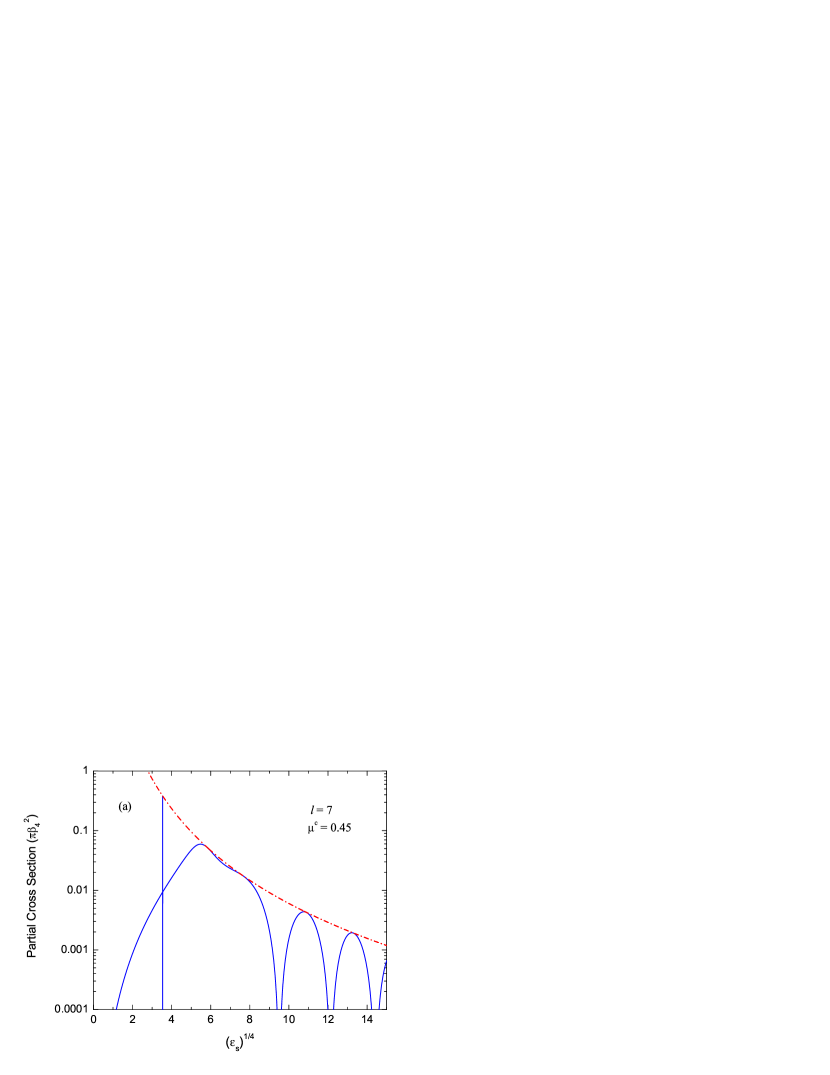
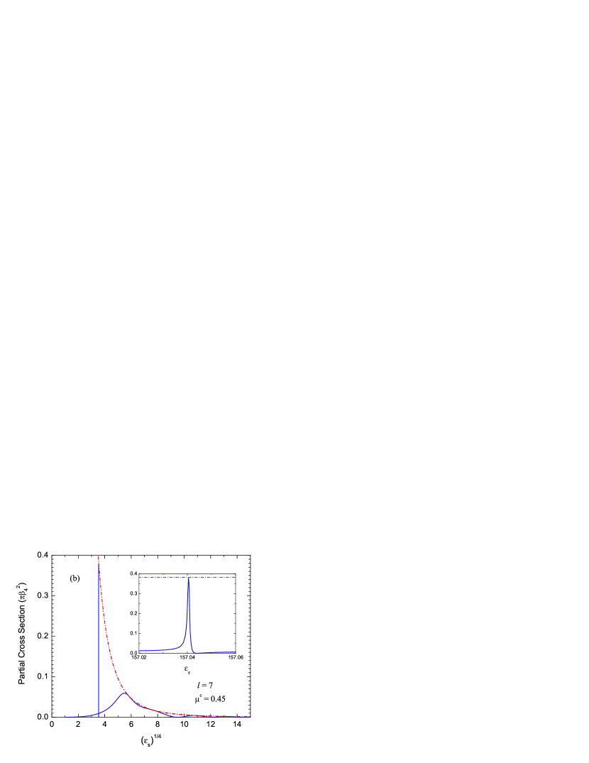
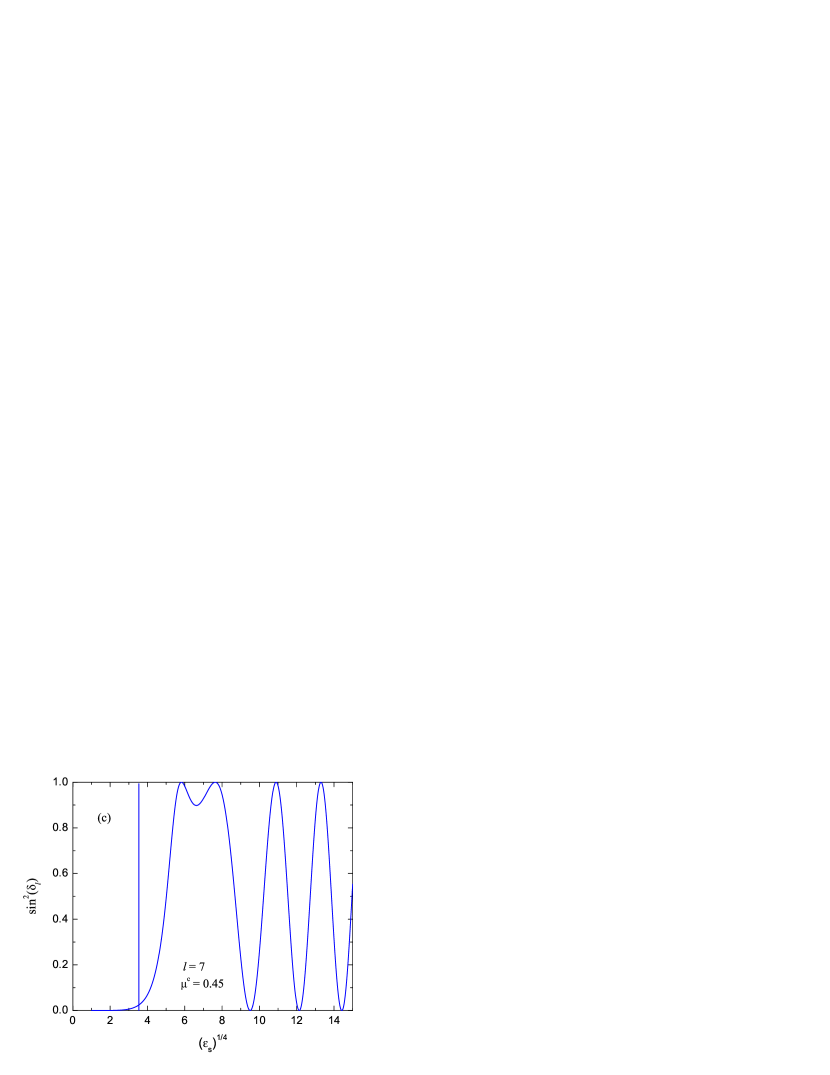
Figure 5: (Color online) Scattering characteristics for partial wave $l=7$ with a quantum defect of $\mu^{c}=0.45$. Both (a) and (b) show the partial cross section (solid line), with the dash-dot line representing the unitarity limit (see text) for $l=7$. Figure (a) shows the cross section on a LOG scale. Figure (b) shows it on a linear scale with a close-up of the narrow feature around $(\epsilon_{s})^{1/4}\approx 3.54$. Figure (c) shows the corresponding $\sin^{2}\delta_{l}$. The set of energies at which the cross section touches the unitarity limit, or $\sin^{2}\delta_{l}$ reaches 1, define the resonance spectrum to be discussed in Sec. III.2.2.

Figure 5 illustrates some of the scattering characteristics for $n=4$ in partial wave $l=7$. It assumes an energy-independent quantum defect of $\mu^{c}(\epsilon,l=7)=0.45$, corresponding to an energy-independent $K^{c}(\epsilon,l=7)\approx-1.37638$ and a $K^{c0}_{l=7}\approx-0.158384$. It is an example used here to motivate the concept of the resonance spectrum and to illustrate the existence of multiple shape resonances for sufficiently large $l$. Both were discussed briefly in Ref. Gao (2010a), and will be discussed in more detail in later sections.

Figure 5(a) shows, on a LOG scale, the partial scattering cross section

$$\sigma_{l}/(\pi\beta_{4}^{2})=[4(2l+1)/\epsilon_{s}]\sin^{2}\delta_{l}\;,$$

for $l=7$, over a range of energies of $0<\epsilon_{s}<50625$ or $0<\epsilon_{s}^{1/4}<15$. Figure 5(b) shows the same cross section on a linear scale, with a closer look at the narrow structure around $\epsilon_{s}^{1/4}\approx 3.54$ ($\epsilon_{s}\approx 157$). Figure 5(c) shows, instead of the partial cross section, the corresponding $\sin^{2}\delta_{l}=|S_{l}-1|^{2}/4$, where $S_{l}=e^{i2\delta_{l}}$ is the single-channel $S$ matrix Gao (2008); Taylor (2006). The $\sin^{2}\delta_{l}$ is basically the partial cross section scaled by its unitarity limit, given by $\sigma^{\mathrm{max}}_{l}/(\pi\beta_{4}^{2})=4(2l+1)/\epsilon_{s}=60/\epsilon_{s}$ for $l=7$. Together, they show that there are considerable structures in scattering. The structures at higher energies are less prominent in the cross section, but only because of the constraint of the unitarity limit. With proper scaling, of both energy and the cross section, there is little difference among the last 4 structures shown in Fig. 5.

Without the concepts of resonance spectrum, width function, and diffraction resonance Gao (2010a), the structures shown in Fig. 5 are easily missed, or unexplained. Potential existence of narrow resonances, such as the first one in Fig. 5, is a general characteristic of low-energy heavy particle (anything other than the electron) neutral-neutral and charge-neutral scattering. Without the resonance spectrum identifying the existence and the locations of such resonances, a standard numerical calculation, which is always performed on a discrete energy mesh, can easily miss some or all of them. They also occur far below the barrier where numerical stability becomes a problem. The concept of the diffraction resonance will help to distinguish the last three resonances from the first two, and the width function will help to provide precise characterizations of all resonances. They will be discussed in Secs. III.3 and IV.1.

III.1.2 Scattering at negative energies

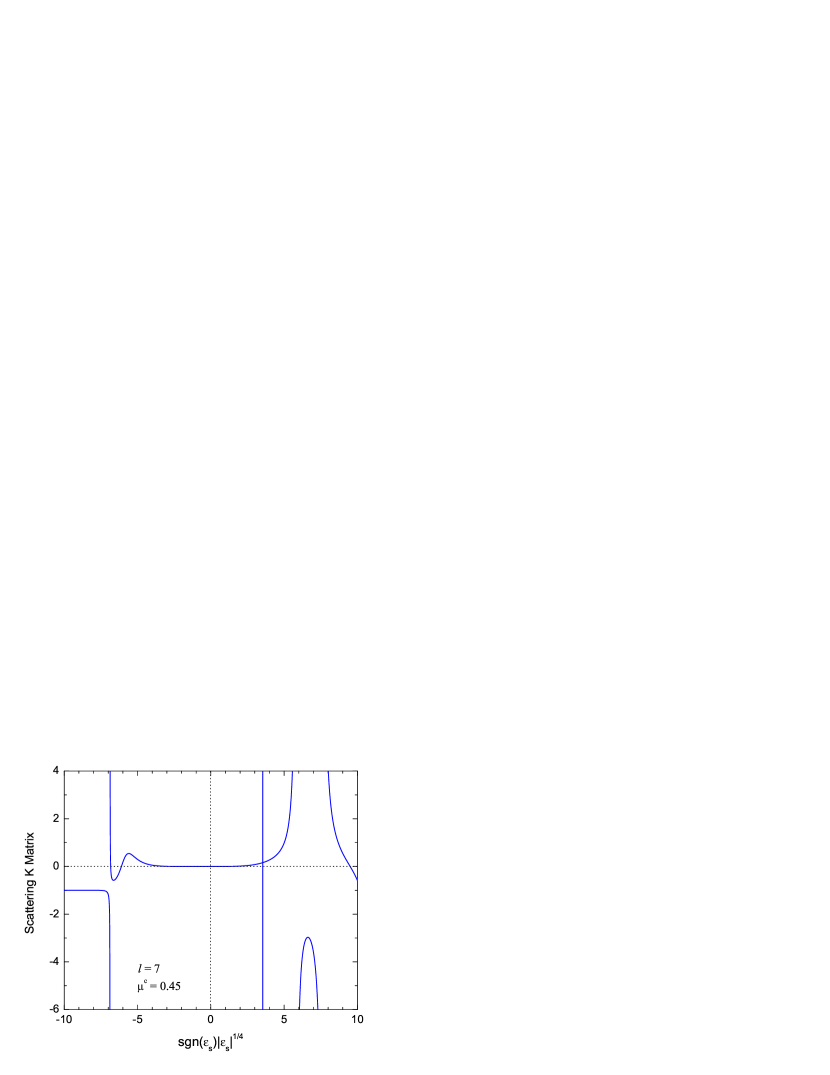
Figure 6: (Color online) An illustration of the generalized $K$ matrix, $\widetilde{K}_{l}$, for scattering at negative energies, together with the corresponding $K_{l}$ for positive energies, for partial wave $l=7$ and $\mu^{c}=0.45$.

In Ref. Gao (2008), we introduced, for negative energies, the generalized $K$ matrix, $\widetilde{K}_{l}$, given in QDT formulation by

$$\widetilde{K}_{l}= \frac{W^{c(n)}_{f-}+(-1)^{l}W^{c(n)}_{f+}-K^{c}[W^{c(n)}_{g-}+(-1)^{l}W^{c(n)}_{g+}]}{W^{c(n)}_{f-}-(-1)^{l}W^{c(n)}_{f+}-K^{c}[W^{c(n)}_{g-}-(-1)^{l}W^{c(n)}_{g+}]}\;,$$ (79)

$$= \frac{\sin(\Phi^{c(n)}_{l}+\delta^{\mathrm{sr}})+(-1)^{l}(D^{c(n)}_{l})^{2}\sin(\Phi^{c(n)}_{l}-\Theta^{c(n)}_{l})\sin(\Theta^{c(n)}_{l}+\delta^{\mathrm{sr}})}{\sin(\Phi^{c(n)}_{l}+\delta^{\mathrm{sr}})-(-1)^{l}(D^{c(n)}_{l})^{2}\sin(\Phi^{c(n)}_{l}-\Theta^{c(n)}_{l})\sin(\Theta^{c(n)}_{l}+\delta^{\mathrm{sr}})}\;.$$ (80)

where $W^{c(n)}_{xy}$, $\Phi^{c(n)}_{l}$, $D^{c(n)}_{l}$, and $\Theta^{c(n)}_{l}$ for $n=4$ are the QDT functions given in Sec. II.

The $\widetilde{K}_{l}(\epsilon<0)$ is a generalization of the $K_{l}(\epsilon>0)=\tan\delta_{l}$ to negative energies. It is well defined for all negative energies and give a more complete characterization of the negative energy states than merely the bound spectrum. This quantity, together with the concept of resonance spectrum Gao (2010a), makes our understanding of two-body interactions more symmetric and more complete for both positive and negative energies. The bound spectrum is contained within $\widetilde{K}_{l}(\epsilon<0)$ as the solutions of $\widetilde{K}_{l}=-1$. The resonance spectrum is contained within $K_{l}(\epsilon>0)$, as solutions of $K_{l}(\epsilon>0)=\infty$. The generalized $K$ matrix has applications in interaction in reduced dimensions Chen and Gao (2007), and in few-body Khan and Gao (2006) and many-body physics Gao (2004a, 2005).

In Fig. 6, we illustrate the $\widetilde{K}_{l}(\epsilon<0)$, together with $K_{l}(\epsilon>0)$, for the case of $l=7$ and $\mu^{c}=0.45$. The positive energy part is the $K_{l}$ corresponding to the scattering properties illustrated in Fig. 5. Figure 6 also serves to show the general feature that $\widetilde{K}_{l}$ evolves continuously to $K_{l}$ at zero energy. This evolution is however not analytic at $\epsilon=0$, with different functional representations in $\epsilon<0$ and $\epsilon>0$, respectively.

III.2 Spectrum

III.2.1 Bound spectrum

In single-channel QDT, the bound spectrum of a two-body system with $-1/r^{n}$ ($n>2$) type of long-range potential is given rigorously by the solutions of Gao (2001, 2008)

$$\chi^{c(n)}_{l}(\epsilon_{s})=K^{c}(\epsilon,l)\;.$$ (81)

Here $\chi^{c(n)}_{l}=W^{c(n)}_{f-}/W^{c(n)}_{g-}=-\tan\Phi^{c(n)}_{l}$ is a universal function of $\epsilon_{s}$, uniquely determined by $n$ and $l$. A conceptually useful equivalent of Eq. (81) is $\Phi^{c(n)}+\delta^{\mathrm{sr}}=j\pi$, where $j$ is an integer.

For $n=4$, we have, from the $W^{c}$ matrix of Sec. II,

$$\chi^{c(4)}_{l}=\tan(\pi\nu/2)\frac{1+M_{\epsilon_{s}l}^{2}}{1-M_{\epsilon_{s}l}^{2}}\;.$$ (82)

The resulting bound spectrum can be represented in a number of different manner as to be discussed in Sec. III.2.3.

III.2.2 Resonance spectrum

In Ref. Gao (2010a), we introduced the concept of resonance spectrum as a set of energies at which $\sin^{2}\delta_{l}=1$, namely the energies at which the partial scattering cross section reaches its unitarity limit, as illustrated in Fig. 5. Such locations can be determined as the roots of the denominator in Eq. (76). Defining a generalized $\chi^{c(n)}_{l}$ function for positive energies as $\widetilde{\chi}^{c(n)}_{l}(\epsilon_{s})\equiv Z^{c(n)}_{fs}/Z^{c(n)}_{gs}$, the resonance positions can be formulated in a manner similar to the bound spectrum, as the solutions of

$$\widetilde{\chi}^{c(n)}_{l}(\epsilon_{s})=K^{c}(\epsilon,l)\;.$$ (83)

For $n=4$, we have from the $Z^{c}$ matrix of Sec. II,

$$\widetilde{\chi}^{c(4)}_{l}=\tan(\pi\nu/2)\frac{1-(-1)^{l}M_{\epsilon_{s}l}^{2}\tan[\pi(\nu-\nu_{0})/2]}{1+(-1)^{l}M_{\epsilon_{s}l}^{2}\tan[\pi(\nu-\nu_{0})/2]}\;.$$ (84)

The $\widetilde{\chi}^{c(n)}_{l}$ function can be regarded as an extension of the $\chi^{c(n)}_{l}$ function to positive energies. They evolve continuously, but not analytically, into each other across $\epsilon_{s}=0$, with

$$\lim_{\epsilon_{s}\rightarrow 0-}\chi^{c(4)}_{l}=\lim_{\epsilon_{s}\rightarrow 0+}\widetilde{\chi}^{c(4)}_{l}=\tan(\pi\nu_{0}/2)=(-1)^{l}\;.$$

The $\widetilde{\chi}^{c(n)}_{l}$ function can be further used to define a phase $\widetilde{\Phi}^{c(n)}_{l}$, by $\widetilde{\chi}^{c(n)}_{l}=-\tan\widetilde{\Phi}^{c(n)}_{l}$, as an extension of the quantum phase $\Phi^{c(n)}_{l}$ to positive energies. In terms of $\widetilde{\Phi}^{c(n)}_{l}$, a conceptually useful equivalent of Eq. (83) is $\widetilde{\Phi}^{c(n)}+\delta^{\mathrm{sr}}=j\pi$, where $j$ is an integer. It is again a natural extension of the bound spectrum.

Similar to a bound spectrum, which describes, over a set of discrete energies, the rise of a phase from zero to a finite value at the threshold, a resonance spectrum describes its subsequent evolution (eventually) back towards zero. It also describes the evolution of a bound state into continuum, and the evolution of a resonance into a bound state. The potential existence of extremely narrow shape resonances for long-range interactions with $n>2$, as illustrated in Fig. 5 is another motivation for the introduction of resonance spectrum. The mathematical and practical necessity for such a concept will be discussed further in later sections.

III.2.3 Representations of the spectra

Figure 7: (Color online) One representation of the spectra for two-body quantum systems with $-1/r^{4}$ type of interactions, including both the bound spectra for $\epsilon_{s}<0$, where the curves plotted are the $\chi^{c(4)}_{l}$, and the resonance spectra for $\epsilon_{s}>0$, where the curves plotted are the $\widetilde{\chi}^{c(4)}_{l}$. For any two-body quantum system with $-1/r^{4}$ type of long-range potential, the bound spectra and the resonance spectra are given by the cross points between the curves plotted and a set of curves representing $K^{c}(\epsilon,l)$ for different partial waves $l$. For systems such as ion-atom, $K^{c}(\epsilon,l)$ is approximately an energy- and partial-wave-independent constant, allowing the determination of the entire rovibrational spectra, and the resonance spectra, from a single parameter. The curves representing $K^{c}(\epsilon,l)$ for different $l$ all appear in this case as a single horizontal line, as illustrated in the figure. The $\widetilde{\chi}^{c(4)}_{l}$ functions evolves from a piecewise monotonically decreasing function of energy to a piecewise monotonically increasing function of energy at the critical scaled energy $B_{c}(l)$.

Figure 8: (Color online) Representation of the spectra as the cross points between the curves plotted, $\chi^{\mu(4)}_{l}(\epsilon_{s})$ for $\epsilon_{s}<0$ and $\widetilde{\chi}^{\mu(4)}_{l}(\epsilon_{s})$ for $\epsilon_{s}>0$, and a set of curves representing $\mu^{c}(\epsilon,l)$ for different partial waves $l$. For ion-atom interaction, $\mu^{c}(\epsilon,l)$ is approximately an energy- and partial-wave-independent constant, allowing the determination of the entire spectra from a single parameter, as illustrated by a horizontal line in the figure corresponding to $\mu^{c}=0.45$.

There are a number of different representations of both the bound and the resonance spectra, corresponding to descriptions of the short-range physics using different parameters such as $K^{c}(\epsilon,l)$, $\mu^{c}(\epsilon,l)$, or $K^{c0}_{l}(\epsilon)$. They have different utilities and applications, and offer different physical insights.

$K^{c}$ representation: Figure 7 gives the most direct representation of Eqs. (81) and (83). It represents the bound spectra as the crossing points between the $K^{c}(\epsilon,l)$ and the $\chi^{c(n)}_{l}$ function for $\epsilon<0$, and the resonance spectra as the crossing points between the $K^{c}(\epsilon,l)$ and $\widetilde{\chi}^{c(n)}_{l}$ function for $\epsilon>0$. It is the base representation that is the most convenient for most computational purposes.

For negative energies, $\chi^{c(n)}_{l}$ is a piecewise monotonically decreasing function of energy with $d\widetilde{\chi}^{c(n)}_{l}/d\epsilon_{s}<0$. It evolves into $\widetilde{\chi}^{c(n)}_{l}$ at zero energy. For positive energies, $\widetilde{\chi}^{c(n)}_{l}$ continues to be piecewise monotonically decreasing until it reaches the critically scaled energy $B_{c}(l)$ defined by $\left.d\widetilde{\chi}^{c(n)}_{l}/d\epsilon_{s}\right|_{B_{c}(l)}=0$. Above $B_{c}(l)$, $\widetilde{\chi}^{c(n)}_{l}$ evolves into a piecewise monotonically increasing function of energy with $d\widetilde{\chi}^{c(n)}_{l}/d\epsilon_{s}>0$. In terms of the closely related quantum phase, the critical scaled energy $B_{c}(l)$ corresponds to the scaled energy at which the quantum phase evolves from monotonically increasing to monotonically decreasing with energy.

$\mu^{c}$ representation: In the second representation of the spectrum, the short-range physics is described using the $\mu^{c}(\epsilon,l)$ parameter. Specifically, Eqs. (81) and (83) can be rewritten as

$$\chi^{\mu(n)}_{l}(\epsilon_{s})=\mu^{c}(\epsilon,l)\;,$$ (85)

for the bound spectrum, and

$$\widetilde{\chi}^{\mu(n)}_{l}(\epsilon_{s})=\mu^{c}(\epsilon,l)\;,$$ (86)

for the resonance spectrum. Here $\chi^{\mu}_{l}$ is defined in terms of $\chi^{c}_{l}$ as $\chi^{\mu}_{l}=[\tan^{-1}(\chi^{c}_{l})-\pi b/2]/\pi$, in which $\tan^{-1}(\chi^{c}_{l})$ is taken to be within a range of $\pi$ of $[\pi b/2,\pi+\pi b/2)$, where $b=1/(n-2)$. The $\widetilde{\chi}^{\mu}_{l}$ is defined in terms of $\widetilde{\chi}^{c}_{l}$ in a similar manner. In this representation, the spectra are given by the crossing points between the $\mu^{c}(\epsilon,l)$ and the $\chi^{\mu(n)}_{l}$ function for $\epsilon<0$, and $\widetilde{\chi}^{\mu(n)}_{l}$ function for $\epsilon>0$, as illustrated in Fig. 8 for $l=5$-$9$. This representation is convenient for the visualization of the semiclassical limit Le Roy and Bernstein (1970); Flambaum et al. (1999); Friedrich and Trost (2004) and for understanding the structure of the rovibrational states around the threshold and the corresponding classification of molecules (molecular ions to be more precise here) Gao (2004b). Similar to $\widetilde{\chi}^{c(n)}_{l}$, the $\widetilde{\chi}^{\mu(n)}_{l}$ function evolves from being monotonically decreasing function of energy to being monotonically increasing function of energy at $B_{c}(l)$.

The semiclassical limit corresponds to regions in Fig. 8 where $\chi^{\mu}_{l}$ (or $\widetilde{\chi}^{\mu}_{l}$) becomes a set of equally-spaced parallel straight lines versus $(-\epsilon_{s})^{1/4}$ for $\epsilon<0$ (versus $\epsilon_{s}^{1/4}$ for $\epsilon>0$). The QDT, being an exact quantum theory, thus also provides a framework for testing various semiclassical approximations Gao (1999b) such as the WKB approximation Le Roy and Bernstein (1970); Flambaum et al. (1999); Friedrich and Trost (2004). From Fig. 8, it is clear that the greater the $l$, the greater the range of energies around the threshold in which the WKB approximation fails. This range is characterized by the quantum order parameter of Sec. II, and grows as $l^{4}$ both below and above the threshold. In the quantum region of negative energies, the number of states is reduced compared to what is to be expected from the WKB theory Le Roy and Bernstein (1970); Flambaum et al. (1999); Friedrich and Trost (2004). They are pushed into the quantum region above the threshold.

Figure 9: (Color online) Representation of the spectra as the cross points between the curves plotted, $\chi^{c0(4)}_{l}(\epsilon_{s})$ for $\epsilon_{s}<0$ and $\widetilde{\chi}^{c0(4)}_{l}(\epsilon_{s})$ for $\epsilon_{s}>0$, and a set of curves representing $K^{c0}_{l}(\epsilon)$ for different partial waves $l$. Unlike the $K^{c}(\epsilon,l)$ and the $\mu^{c}(\epsilon,l)$ parameters, $K^{c0}_{l}(\epsilon)$ is generally different for different $l$. For cases, such as ion-atom interactions, where $K^{c}$ and $\mu^{c}$ are approximately energy- and partial-wave-independent, there are approximately two related energy-independent $K^{c0}_{l}$s given by Eq. (74) or (75), with one describing all even partial waves and one describing all odd partial waves. For the example of $\mu^{c}=0.45$, $K^{c0}_{l}\approx 6.31375$ for all even partial waves, and $K^{c0}_{l}\approx-0.158384$ for all odd partial waves, as illustrated by two horizontal lines.

$K^{c0}$ representation: The third representation of the spectra corresponds to the description of the short-range physics using the $K^{c0}_{l}$ parameter. Eqs. (81) and (83) can be rewritten as

$$\chi^{c0(n)}_{l}(\epsilon_{s})=K^{c0}_{l}(\epsilon)\;,$$ (87)

for bound spectrum, and

$$\widetilde{\chi}^{c0(n)}_{l}(\epsilon_{s})=K^{c0}_{l}(\epsilon)\;,$$ (88)

for the resonance spectrum. Here

$$\chi^{c0(n)}_{l}(\epsilon_{s})=\frac{\chi^{c(n)}_{l}(\epsilon_{s})-\tan(\pi\nu_{0}/2)}{1+\tan(\pi\nu_{0}/2)\chi^{c(n)}_{l}(\epsilon_{s})}\;.$$ (89)

$$\widetilde{\chi}^{c0(n)}_{l}(\epsilon_{s})=\frac{\widetilde{\chi}^{c(n)}_{l}(\epsilon_{s})-\tan(\pi\nu_{0}/2)}{1+\tan(\pi\nu_{0}/2)\widetilde{\chi}^{c(n)}_{l}(\epsilon_{s})}\;.$$ (90)

For $n=4$, we obtain

$$\chi^{c0(4)}_{l}=\frac{\tan(\pi\Delta\nu/2)+(-1)^{l}M_{\epsilon_{s}l}^{2}}{1+(-1)^{l}M_{\epsilon_{s}l}^{2}\tan(\pi\Delta\nu/2)}\;,$$ (91)

$$\widetilde{\chi}^{c0(4)}_{l}=\tan(\pi\Delta\nu/2)\frac{1-M_{\epsilon_{s}l}^{2}}{1-M_{\epsilon_{s}l}^{2}\tan^{2}(\pi\Delta\nu/2)}\;.$$ (92)

Figure 9 illustrates this representation of the spectra. It is the most convenient representation for developing QDT expansion around the threshold Gao (2009), and for understanding the relationship between bound-state or resonance positions and the scattering length (see Sec. IV.2). All three representations of the spectra are general representations since $K^{c}(\epsilon,l)$, $\mu^{c}(\epsilon,l)$, and $K^{c0}_{l}(\epsilon)$ are well defined at all energies and for all partial waves. Similar to $\widetilde{\chi}^{c(n)}_{l}$ and $\widetilde{\chi}^{\mu(n)}_{l}$, the $\widetilde{\chi}^{c0(n)}_{l}$ function evolves from monotonically decreasing below $B_{c}(l)$ to monotonically increasing above $B_{c}(l)$.

Table 1: Energy bins for partial waves $l=5$ through $l=9$. The numbers in the parenthesis represent powers of ten. The $i$-th bound state of angular momentum $l$, with $i=1$ corresponding to the least-bound state, is to be found within $B_{-i}(l)\leq\epsilon_{s}<B_{-i+1}(l)$ for $i>1$, and within $B_{-1}(l)\leq\epsilon_{s}<0$ for $i=1$. Shape resonances of angular momentum $l$ can only exist between $0<\epsilon_{s}<B_{c}(l)$. The $i$-th diffraction resonance of angular momentum $l$, defined as a resonance with negative width, is to be found within $B_{i-1}(l)<\epsilon_{s}\leq B_{i}(l)$ for $i\geq 1$. A zeroth diffraction resonance may exist within $B_{c}(l)<\epsilon_{s}\leq B_{0}(l)$, depending on the quantum defect.

$B_{x}$	$l=5$	$l=6$	$l=7$	$l=8$	$l=9$
$B_{4}$	7.6023(4)	1.0928(5)	9.8278(4)	1.3698(5)	1.8587(5)
$B_{3}$	4.5573(4)	6.8266(4)	5.9353(4)	8.5880(4)	1.2030(5)
$B_{2}$	2.4932(4)	3.9430(4)	3.2379(4)	4.9310(4)	7.2101(4)
$B_{1}$	1.1826(4)	2.0212(4)	1.4762(4)	2.4382(4)	3.8074(4)
$B_{0}$	4.2509(3)	8.3146(3)	3.8643(3)	8.1816(3)	1.5005(4)
$B_{c}$	5.9473(2)	1.0880(3)	1.8636(3)	3.0457(3)	4.7668(3)
$B_{-1}$	-3.6177(3)	-5.2716(3)	-7.3558(3)	-9.9186(3)	-1.3008(4)
$B_{-2}$	-1.4428(4)	-1.9668(4)	-2.5999(4)	-3.3520(4)	-4.2327(4)
$B_{-3}$	-3.7224(4)	-4.8531(4)	-6.1818(4)	-7.7233(4)	-9.4923(4)
$B_{-4}$	-7.7955(4)	-9.8375(4)	-1.2189(5)	-1.4869(5)	-1.7899(5)

There are many applications of these spectra, which are the equivalents and the generalizations of the atomic Rydberg formula to charge-neutral quantum systems. They relate bound spectrum to scattering and vice versa Gao (1998b, 2001), and provide a systematic understanding for both. One such application is the concept of energy bins Gao (2000); Chin et al. (2010); Gao (2010a): the ranges of energies over which a bound or a resonance state is to be found. They have been given for the first few partial waves, $l=0$-$4$, in Ref. Gao (2010a). Table 1 gives the bins for higher partial waves $l=5$-$9$. In all representations of the spectra, they are determined by the set of scaled energies at which the relevant $\chi_{l}$ function has evolved back to its value at the threshold. In terms of the quantum phase due to the long-range potential, $\Phi^{c(n)}_{l}$ and $\widetilde{\Phi}^{c(n)}_{l}$, they correspond to a set of scaled energies at which the quantum phase differs from its value at the threshold by an integer multiple of $\pi$. Even in cases with substantial energy variations in the short-range parameter, the bins still give the number of states due to the long-range potential.

The energy bin concept Gao (2000); Chin et al. (2010); Gao (2010a) is useful not only in single-channel but also in multichannel formulations Gao et al. (2005); Gao (2011b), where it can be used, for instance, to estimate the number of Fano-Feshbach resonances. A detailed example will be given in a separate publication on MQDT for ion-atom interactions. Further applications of the spectra will be discussed in Secs. IV and V. We point out that for the $s$ wave bound states, Raab and Friedrich have developed a quantization rule by extrapolating between the quantum threshold behavior and the semiclassical behavior Raab and Friedrich (2009).

III.3 QDT description of scattering resonances

The resonance spectrum gives only resonance positions. The QDT equation for scattering, Eq. (76), contains additional information on scattering resonances including their widths and backgrounds that can be further extracted.

Around a scattering resonance located at $\epsilon_{sl}$, which is one of the solutions of Eq. (83), or equivalently Eq. (86) or (88), the scattering $K$ matrix as given by Eq. (76) can be written as

$$K_{l}(\epsilon)=K_{\text{bg}l}(\epsilon)-\frac{1}{2}\frac{\Gamma_{sl}}{\epsilon_{s}-\epsilon_{sl}}\;,$$ (93)

where both the background term, $K_{\text{bg}l}(\epsilon)$, and the scaled width $\Gamma_{sl}$ can be given in terms of a single function $f_{\Gamma}$ defined by

$$f_{\Gamma}\equiv\frac{\left(Z^{c(n)}_{gc}K^{c}-Z^{c(n)}_{fc}\right)/Z^{c(n)}_{gs}}{\left[\left(\widetilde{\chi}^{c(n)}_{l}-K^{c}\right)/(\epsilon_{s}-\epsilon_{sl})\right]}\;.$$ (94)

Specifically,

$$K_{\text{bg}l}(\epsilon) =\frac{f_{\Gamma}(\epsilon_{s})-f_{\Gamma}(\epsilon_{sl})}{\epsilon_{s}-\epsilon_{sl}}\;,$$ (95)

$$\Gamma_{sl} =-2f_{\Gamma}(\epsilon_{sl})\;.$$ (96)

The function $f_{\Gamma}$ is regular at $\epsilon_{sl}$, with a value of $f_{\Gamma}(\epsilon_{sl})=\lim_{\epsilon_{s}\rightarrow\epsilon_{sl}}f_{\Gamma}(\epsilon_{s})$. Using the property of $\det(Z^{c(n)})=1$ Gao (2008), we obtain

$$\Gamma_{sl}=-2\left\{\left[Z^{c(n)}_{gs}(\epsilon_{sl},l)\right]^{2}\left.\left[\frac{d\widetilde{\chi}^{c(n)}_{l}}{d\epsilon_{s}}-\frac{dK^{c}}{d\epsilon_{s}}\right]\right|_{\epsilon_{sl}}\right\}^{-1}\;.$$ (97)

For most true single-channel problems, the energy dependence of the $K^{c}$ is negligible, and $\Gamma_{sl}$ reduces to a universal function of the scaled resonance position, given by

$$\gamma^{(n)}_{sl}(\epsilon_{sl})=-2\left\{\left.\frac{d\widetilde{\chi}^{c(n)}_{l}}{d\epsilon_{s}}\right|_{\epsilon_{sl}}\left[Z^{c(n)}_{gs}(\epsilon_{sl},l)\right]^{2}\right\}^{-1}\;.$$ (98)

It will be called the universal width function. It is a function of the scaled resonance position that is uniquely determined by $n$ and $l$, and is given in terms of the QDT functions defined earlier.

This QDT description of scattering resonance is generally applicable to any long-range potential of the form of $-C_{n}/r^{n}$ with $n>2$. The $\gamma^{(n)}_{sl}$ for $n=4$ is discussed further in the next section. The more general expression for the scaled width, Eq. (97), will be useful in cases where the energy dependence of $K^{c}$ is not negligible. These include some cases of electron-atom interactions, and maybe more importantly, some cases corresponding to effective single-channel descriptions of Fano-Feshbach resonances, for which the effective $K^{c}$ parameter can have substantial energy dependence around a narrow resonance Gao (2011b).

IV Single-channel universal behaviors for $-1/r^{4}$ potential

Embedded in the QDT descriptions of spectra and scattering resonances are a set of universal properties followed in varying degrees by virtually all single-channel charge-neutral systems in a range of energies around the threshold. They correspond to a set of conclusions that can be drawn from the QDT formulation under the assumption that the short-range parameter, $K^{c}(\epsilon,l)$, $\mu^{c}(\epsilon,l)$, or $K^{c0}_{l}(\epsilon)$, is independent of energy. Mathematically, they can also be defined rigorously as the universal property at length scale $\beta_{4}$, emerging in the limit of other length scales going to zero in comparison Gao (2004a, 2005); Khan and Gao (2006). Among these properties, there is a subset of conclusions that can be drawn under the further assumption that the parameter $K^{c}(\epsilon,l)$ or $\mu^{c}(\epsilon,l)$ [but not $K^{c0}_{l}(\epsilon)$] are not only independent of energy, but also independent of $l$. This subset is applicable, e.g., to ion-atom interactions, for which they imply a set of relations among interactions in different partial waves Gao (2001, 2000, 2004b); Li and Gao (2012). They are not applicable to electron- or positron-atom interactions, for which the relationship between interactions in different $l$ depends on the details of the short-range potential.

IV.1 Universal width function

Figure 10: (Color online) Illustrations of the universal width function for $l=6$ and 7. The width diverges at the critical scaled energy $\epsilon_{sl}=B_{c}(l)$. It is positive below $B_{c}(l)$, in the region corresponding to shape resonances, and negative above $B_{c}(l)$, in the region corresponding to diffraction resonances.

We begin our discussion of universal behaviors with the universal width function, as it is required for further understanding and interpretation of the resonance spectra. Under the assumption of the short-range parameter being independent of energy, the scaled width $\Gamma_{sl}$ of a scattering resonance, given generally by Eq. (97), reduces to the universal width function $\gamma_{sl}$ given by Eq. (98). It implies that while the position of a scattering resonance depends generally on the short-range parameter such as $K^{c}$, the width of the resonance, as a function of the scaled resonance position $\epsilon_{sl}$, follows a universal behavior for an energy-independent $K^{c}$.

The most important characteristic of the universal width function is that it changes sign and diverges at a critical scaled energy $B_{c}(l)$. Below $B_{c}(l)$, $\widetilde{\chi}^{c(n)}_{l}$ is a piecewise monotonically decreasing function of energy with $d\widetilde{\chi}^{c(n)}_{l}/d\epsilon_{s}<0$, which, from Eq. (98), implies that all resonances occurring in the region of $0<\epsilon_{s}<B_{c}(l)$ have positive widths. Above $B_{c}(l)$, $\widetilde{\chi}^{c(n)}_{l}$ is piecewise monotonically increasing with $d\widetilde{\chi}^{c(n)}_{l}/d\epsilon_{s}>0$, implying that all resonances above $B_{c}(l)$ have negative widths.

Resonances of positive width are called shape resonances, consistent with the standard convention. Resonances of negative width are called diffraction resonances. Their distinction can be understood through the concept of the time delay and the closely related concept of the change of the density-of-states due to interaction Wigner (1955); Taylor (2006). Let $\Delta t_{s}\equiv\Delta t/s_{t}$ be the scaled time delay, where $s_{t}=\hbar/s_{E}$ is the time scale associated with the length scale $\beta_{n}$. Let $D_{sl}\equiv D_{l}/(1/s_{E})$ be the scaled change of the density-of-states due to interaction. They are related, and are given by

$$\Delta t_{s}=2\pi D_{sl}=2\frac{d\delta_{l}}{d\epsilon_{s}}=\frac{2}{1+K_{l}^{2}}\frac{dK_{l}}{d\epsilon_{s}}\;.$$ (99)

It is clear from this equation and Eq. (93) that a resonance of positive width corresponds to a time delay Wigner (1955); Taylor (2006) and an enhanced density-of-states, while a resonances of negative width (diffraction resonance) corresponds to a time advance Wigner (1955); Hammer and Lee (2010) and a reduced (negative change) density-of-states. For a long-range interaction of the type of $1/r^{n}$ with $n>3$, the total number of states is not changed by the interaction, as is reflected in the Levinson theorem Levinson (1949); Joachain (1975). Both the bound states and the shape-resonance states can be regarded as states taken from the continuum by the interaction. The diffraction resonances, which correspond to negative changes of the density-of-states, give the origin of the bound states and the shape-resonance states, namely where in continuum such states come from.

The proceeding discussion on the characterization of scattering resonances are applicable to arbitrary $-1/r^{n}$ potential with $n>3$. For the specific case of $n=4$, Figure 10 gives an illustration of both the width function and the concept of $B_{c}(l)$ for partial waves $l=6$ and 7. Unlike the width for a shape resonance which can be infinitely small, the absolute width for a diffraction resonance cannot be infinitely small. It has a lower limit as required by causality Wigner (1955); Hammer and Lee (2010).

Figure 11: (Color online) A closer look at the bound and resonance spectra for $l=6$ and $7$ in the $K^{c}$ representation, showing the potential existence of two shape resonances for $l\geq 7$. For $l\leq 6$, an energy-independent $K^{c}$, represented by a horizontal line, can have only a single crossing point with $\chi^{c}_{l}$ within the region of $0<\epsilon_{s}<B_{c}(l)$, regardless the value of $K^{c}$. For $l=7$ and with proper value of $K^{c}$, there can be two such points, corresponding to two shape resonances. The horizontal line illustrated at $K^{c}\approx-1.37638$ corresponds to $\mu^{c}=0.45$ example of Fig. 5.

The QDT formulations for the spectra, together with the concept of $B_{c}(l)$, also give the maximum number of shape resonances that can exist for a particular $l$. They show, e.g., that the minimum $l$ that can support two shape resonances through the long-range potential is $l=7$. Figure 11 gives a further illustration of the relevant concepts, and the difference in behavior between $l=6$ and $l=7$. In the $K^{c}$ and $\mu^{c}$ representations of the spectra, the maximum number of shape resonances corresponds to the maximum number of crossing points between the relevant $\chi_{l}$ function and a straight line that can exist in the region of $0<\epsilon_{s}<B_{c}(l)$. Figure 11 shows that there can only be one such point for $l\leq 6$, but there can be two such points, depending on the short-range parameter, for $l=7$. Similarly the $\chi_{l}$ functions for larger $l$ show that the minimum $l$ for the existence of 3 shape resonances is $l=19$. For partial wave $0<l<7$, the increase of the quantum phase $\widetilde{\Phi}^{c(n)}_{l}$ from the threshold to $B_{c}(l)$, where it reaches its maximum value, is less than $\pi$. The phase at $B_{0}(l)$ (c.f. Table 1) is the same as its value at the threshold. For $7\leq l<19$, the increase of the quantum phase $\widetilde{\Phi}^{c(n)}_{l}$ from the threshold to $B_{c}(l)$ is between $\pi$ and $2\pi$, and the quantum phase at $B_{0}(l)$ is greater than its value at the threshold by $\pi$. Similar consideration applies to higher partial waves.

Figure 12: (Color online) The critical scaled energies $B_{c}(l)$ and the scaled barrier height $H_{s}(l)$ for different partial waves. It illustrates that both $B_{c}(l)$ and $H_{s}(l)$ have $\sim l^{4}$ type of $l$ dependence. $B_{c}(l)$ is always greater than $H_{s}(l)$, substantially greater for large $l$, implying that a shape resonance can exist at a substantially greater energy above the top of the barrier.

Figure 12 shows the $B_{c}(l)$ for a large number of partial waves, together with the scaled barrier height for a $-1/r^{4}$ potential given by $H_{s}(l)=[l(l+1)]^{2}/4$. It illustrates that (a) both $B_{c}(l)$ and $H_{s}(l)$ have $\sim l^{4}$ type of $l$ dependence, and (b) $B_{c}(l)$ is always greater than $H_{s}(l)$, substantially greater for large $l$, implying that a shape resonance can exist at a substantially greater energy above the top of the barrier.

With the introduction and the interpretation of the universal width function, we can now provide a more complete characterization of the five resonances in Fig. 5. The resonance positions can be predicted from any of the three formulations of the spectrum in Sec. III, and the widths are evaluated from the universal width function. In partial wave $l=7$ with $\mu^{c}(l=7)=0.45$, there are two shape resonances located at $\epsilon_{s}=157.041$, and $\epsilon_{s}=1148.23$, with scaled widths of $1.099\times 10^{-3}$ and $1.851\times 10^{3}$, respectively. They are shape resonances with positive widths. The scaled barrier height for $l=7$ is $H_{s}(l=7)=784$. The narrow shape resonance is substantially below the barrier, and the broad shape resonance is above the barrier and below the $B_{c}(l=7)\approx 1863.58$. The other three resonances are located at $\epsilon_{s}=3390.55,14082.9$, and 31297, with scaled widths of $-6.220\times 10^{3}$, $-8.542\times 10^{3}$, and $-1.362\times 10^{4}$, respectively. They are diffraction resonances with negative widths. We emphasize that without the concept of the diffraction resonance, not all the features in Figure 5 would be accounted for. We further emphasize that from a pure mathematical point of view, any attempt to represent the $K$ matrix, namely the $K_{l}$ function, as a smooth background function plus a set of poles over the entire positive energy range can never ignore poles associated with diffraction resonances. The only difference between these poles and those associated with shape resonances is that they have a residue of a different sign.

IV.2 Universal spectral properties

Figure 13: (Color online) The universal spectra for quantum systems with a $-1/r^{4}$ type of long-range interaction, versus $\mu^{c}(l)$ for $l=5$-$9$. The applicability of each individual curve, which gives the spectrum of a particular partial wave $l$ from the corresponding short-range parameter $\mu^{c}(l)\equiv\mu^{c}(\epsilon=0,l)$, requires only the energy independence of the parameter. For systems such as ion-atom, for which $\mu^{c}(l)$ is approximately independent of $l$, a single $\mu^{c}(l=0)$ gives the entire spectra for all $l$. A similar figure for lower partial waves can be found in Ref. Gao (2010a).

Figure 14: (Color online) The universal spectra for quantum systems with a $-1/r^{4}$ type of long-range interaction, versus $K^{c0}_{l}\equiv K^{c0}_{l}(\epsilon=0)$ for $l=0$-$4$. Since $K^{c0}_{l}$ is related to the generalized scattering length by Eq. (104), this set of curves also represent the spectra as a function of the inverse of a reduced generalized scattering length, $1/(\widetilde{a}_{l}/\bar{a}^{(4)}_{l})$.

Under the assumption that the short-range parameter, $K^{c}(\epsilon,l)$, $\mu^{c}(\epsilon,l)$, or $K^{c0}_{l}(\epsilon)$, being independent of energy, they are constants that can be taken to be their values at the zero energy. Defining $K^{c}(l)\equiv K^{c}(\epsilon=0,l)$, $\mu^{c}(l)\equiv\mu^{c}(\epsilon=0,l)$, and $K^{c0}_{l}\equiv K^{c0}_{l}(\epsilon=0)$, the equations for the spectra can be solved (inverted) to give both the scaled binding energies and the scaled resonance positions, $\epsilon_{sl}$, as a function of a short-range parameter, $K^{c}(l)$, $\mu^{c}(l)$, or $K^{c0}_{l}$. Figures 13 and 14 illustrate the results versus $\mu^{c}(l)$ and $K^{c0}_{l}$, respectively. They are the $-1/r^{4}$ equivalents of the Rydberg formula for the Coulomb interaction, generalized to include also the resonance spectrum. They greatly generalize the well-known result of the effective range theory Schwinger (1947); Blatt and Jackson (1949); Bethe (1949), $\epsilon_{sl=0}\sim-(a_{l=0}/\beta_{4})^{-2}$, for the $s$ wave least-bound state, to more deeply bound states, to all partial waves, and to resonance positions. The representation in terms of $\mu^{c}(l)$, Fig. 13, is the most convenient for a systematic understanding of ion-atom spectra, for which the $\mu^{c}(l)$ has the additional characteristic of being approximately partial-wave-independent. The representation in terms of $K^{c0}_{l}$, Fig. 14, is most convenient for illustrating the dependence of the spectra on the scattering length or the generalized scattering length Gao (2009), as we now explain.

For any potential of the type of $-1/r^{n}$ with $n>3$, the $s$ wave scattering length is well defined (at zero energy), and is related to the other short-range parameters at zero energy through $K^{c}(\epsilon=0,l=0)$ by Gao (2003, 2004b)

$$a_{l=0}/\beta_{n}=\left[b^{2b}\frac{\Gamma(1-b)}{\Gamma(1+b)}\right]\frac{K^{c}(0,0)+\tan(\pi b/2)}{K^{c}(0,0)-\tan(\pi b/2)}\;,$$ (100)

where $b=1/(n-2)$. For $n=4$, this relation reduces to Li and Gao (2012)

$$a_{l=0}/\beta_{4}=\frac{K^{c}(0,0)+1}{K^{c}(0,0)-1}\;.$$ (101)

Combining it with Eq. (74), we have

$$K^{c0}_{l=0}(\epsilon=0)=\frac{1}{a_{l=0}/\beta_{4}}\;.$$ (102)

Equation (102) means that at least for the $s$ wave, Fig. 14 gives in fact a representation of the spectrum as a function of the inverse of a reduced scattering length.

Combining Eqs. (75) and (102) gives

$$a_{l=0}/\beta_{4}=\cot[\pi\mu^{c}(\epsilon=0,l=0)]\;,$$ (103)

which relates the $s$ wave scattering length to the $s$ wave quantum defect evaluated at the zero energy, with the range of $0\leq\mu^{c}(\epsilon=0,l=0)<0.5$ corresponding to positive $s$ wave scattering length, $0.5<\mu^{c}(\epsilon=0,l=0)<1$ corresponding to negative $s$ wave scattering length, and $\mu^{c}(\epsilon=0,l=0)=0.5$ corresponding to the zero $s$ wave scattering length.

For other partial waves, the scattering length is not defined in the conventional sense O’Malley et al. (1961); Levy and Keller (1963). However, in an upcoming publication, we will show that the concept of scattering length can be generalized to all partial waves through the QDT expansion Gao (2009) for the $-1/r^{4}$ potential. This generalized scattering length is related to $K^{c0}_{l}(\epsilon)$ at zero energy by

$$K^{c0}_{l}(\epsilon=0)=\frac{1}{\widetilde{a}_{l}/\bar{a}^{(4)}_{l}}\;,$$ (104)

where $\bar{a}^{(4)}_{l}=\bar{a}^{(4)}_{sl}\beta_{4}^{2l+1}$ is called the mean scattering length for the $-1/r^{4}$ potential in partial wave $l$, with

$$\bar{a}^{(4)}_{sl} = \frac{\pi^{2}}{2^{4l}(2l+1)^{2}[\Gamma(l+1/2)]^{2}}$$ (105)

$$= \frac{(2l+1)^{2}}{[(2l+1)!!]^{4}}\;,$$

being what we call the scaled mean scattering length for the $-1/r^{4}$ potential in partial wave $l$ Gao (2011a). Thus $K^{c0}_{l}$ at the zero energy is the inverse of a reduced generalized scattering length, not only for the $s$ wave, where Eq. (104) reduces to Eq. (102), but for all partial waves. Figure 14 gives the spectrum as a function of this inverse reduced generalized scattering length for all partial waves. The generalized scattering length is related to the quantum defect evaluated at the zero energy, by

$$\widetilde{a}_{l}/\bar{a}^{(4)}_{l}=\left\{\begin{array}[]{ll}\cot[\pi\mu^{c}(\epsilon=0,l)]\;,&l=\text{even}\\ -\tan[\pi\mu^{c}(\epsilon=0,l)]\;,&l=\text{odd}\end{array}\right.\;.$$ (106)

It reduces to Eq. (103) for the $s$ wave.

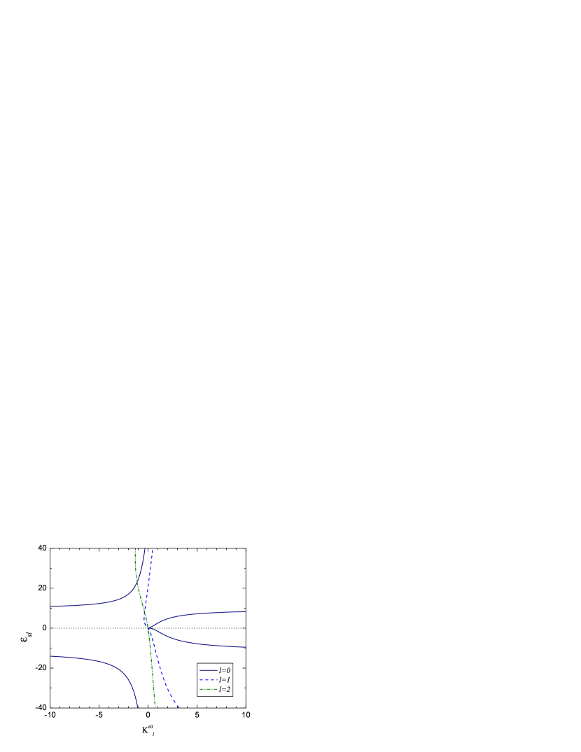
Figure 15: (Color online) A magnified view of a small region of Figure 14 around the threshold, showing the bound state energy and the resonance position $\epsilon_{sl}$ on a linear scale. It is easier to observe on this figure the expected $\epsilon_{sl=0}\sim-(a_{l=0}/\beta_{4})^{-2}$ behavior for the $s$ wave bound state energy around the threshold.

Figure 15 is a magnified view of a small region of Figure 14 around the threshold. It is used to illustrate the expected $\epsilon_{sl=0}\sim-(a_{l=0}/\beta_{4})^{-2}$ behavior for the $s$ wave bound state energy around the threshold.

All universal properties discussed up to this point assume only the energy independence of the short-range parameter. For single-channel ion-atom interactions, the spectra follow closely a set of universal behaviors that are derived under the further assumption that the short-range parameter, $K^{c}(\epsilon,l)$ or $\mu^{c}(\epsilon,l)$ [but not $K^{c0}_{l}(\epsilon)$], is not only independent of energy, but also independent of the partial wave $l$ Gao (2001, 2004b); Li and Gao (2012). In this case, interaction in different partial waves become related. Other than a single overall energy scaling factor $s_{E}$, every aspect of ion-atom interaction, including the entire rovibrational spectrum and all scattering properties in all partial waves, can be determined from a single parameter Gao (2001); Li and Gao (2012).

Some of the consequences on the spectra that emerge for an $l$ independent $\mu^{c}$ or $K^{c}$ have been discussed in Ref. Gao (2004b) in the general context of an arbitrary $-1/r^{n}$ potential with $n>2$. Figure 13, together with Figure 1 of Ref. Gao (2010a), illustrates explicitly how such properties manifest themselves in the spectra for the $-1/r^{4}$ potential. Specifically, they show explicitly the following characteristics of a single-channel ion-atom system. (a) Having a quasibound $s$ state right at the threshold means having a bound state right at the threshold for all even partial waves with $l=0+(n-2)j=2j$ where $j$ is a nonnegative integer. Similarly, having a $p$ wave bound state right at the threshold means having a bound state right at the threshold for all odd partial waves with $l=1+(n-2)j=2j+1$. (b) The least-bound state for a single-channel ion-atom system is either an $s$ state or a $p$ state, depending on the quantum defect Gao (2004b). For systems with $0\leq\mu^{c}<0.5$, corresponding to positive $s$ wave scattering lengths, the least bound state is an $s$ state. For systems with $0.5<\mu^{c}<1$, corresponding to negative $s$ wave scattering lengths, the least bound state is an $p$ state. (c) Systems with a quantum defect smaller than but close to 0.5, correspond to a small positive $s$ wave scattering length, have a set of narrow shape resonances in odd partial waves. Systems with a quantum defect smaller than but close to 1.0, corresponding to a large negative $s$ wave scattering length, have a set of narrow shape resonances in even partial waves.

IV.3 Universal total elastic cross section for single-channel ion-atom scattering

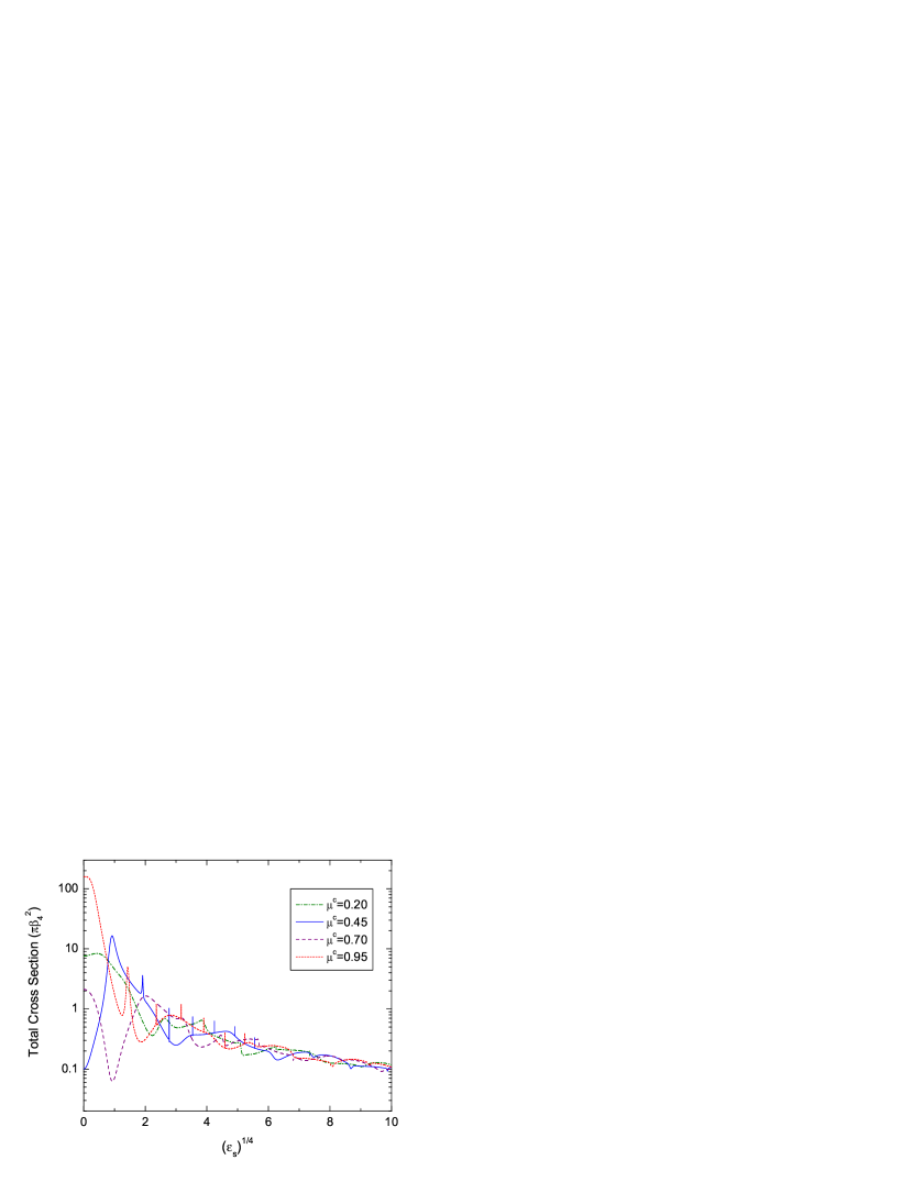
Figure 16: (Color online) Illustrations of universal single-channel ion-atom total elastic cross section. Different systems differ only in scaling as determined by the atomic polarizability, and a single quantum defect $\mu^{c}$, which can be determined from a single experimental measurement of either a resonance position or a bound state energy of a vibrationally highly-excited state. Note the existence of many narrow shape resonances, similar to that illustrated for $l=7$ in Fig. 5, for $\mu^{c}$ smaller than but close to either 0.5 or 1.

For single-channel ion-atom interactions, having a single parameter being able to describe multiple partial waves implies that not only a partial cross section would follow a universal behavior, but also the total cross section Li and Gao (2012). Figure 16 illustrates the universal behavior of the total cross section that is followed in varying degrees by all single-channels ion-atom systems. They include all ¹S+¹S type of ion-atom systems (corresponding to a single ${}^{1}\Sigma$ molecular state), such as a Group IA ion (e.g. Li⁺) or Group IIIA ion (e.g. Al⁺) with Group IIA atoms (e.g. Mg) or Group VIIIA atoms (e.g. Ar). It is also applicable to all ¹S+²S type of ion-atom interactions (a single ${}^{2}\Sigma$ molecular state) provided that the atoms involved are dissimilar, namely has different atomic number $Z$, and the ionization potentials of the atoms involved are such that there is either no charge transfer channel open at low energies or that the transfer cross section is small. The examples include interactions of Group IIA ions with Group VIIIA atoms, such as Mg⁺+Ar, Group IIA ions with Group IIA atoms of a difference species, such as Mg⁺+Ca, Group IIIA ion with Group IA atoms, Group IA atoms with Group IA ion of a different species, such as Li⁺+Na. For sufficiently small energies around the threshold, all such systems differ only in scaling as determined by the atomic polarizability, and a single quantum defect.

Figure 16 further illustrates the potential existence of extremely narrow shape resonances, many of which would almost definitely be missed on any calculation performed on a finite energy mesh. In order not to miss them, one needs first to identify their existence and locations using the resonance spectrum and to calculate their widths using the width function. A special mesh of energies are then generated around the narrow resonance locations using the width information. Cross section calculations performed on the special mesh are added to those on the regular mesh to give the results of Figure 16.

The single-channel universal behavior for ion-atom interaction has been verified through comparison with numerical calculations Li and Gao (2012). The energy range of applicability of the universal behavior, as measure in units of $s_{E}$, is determined by the length scale separation, more specifically by $\beta_{6}/\beta_{4}$, where $\beta_{6}=(2\mu C_{6}/\hbar^{2})^{1/4}$ is the length scale associated with the $-C_{6}/r^{6}$ term of the ion-atom potential, as in $V(r)\sim-C_{4}/r^{4}-C_{6}/r^{6}$. As illustrated in Ref. Li and Gao (2012), this range of energy is typically $10^{5}s_{E}$ if the atom involved is an alkali-metal atom. Beyond this range, accurate QDT calculations will require incorporation of the $l$ dependence of the short-range parameter, as will be illustrated elsewhere.

V Discussions

All equations of this work are formally applicable to both ion-atom and electron-atom or positron-atom interactions. There are however significant differences in how they are actually used in those different contexts, as already mentioned throughout this work. We briefly summarize some of the key differences here for the sake of clarity and future applications.

For ion-atom interactions, $K^{c}$ depends very weakly on energy on a scale of $s_{E}$, due to the fact the $\beta_{4}$ is much greater than other length scales in the system Gao (2010a); Li and Gao (2012). It also depends weakly on the partial wave $l$, a feature that is very important for its application beyond the ultracold regime Li and Gao (2012). For an accurate characterization of low-energy ion-atom interaction, the key difficulty is the sensitive dependence of the short-range parameter and the scattering length on the short-range potential Gao (1996); Li and Gao (2012). This difficulty is overcome in the QDT formulation through direct determination of such parameters from one or a few measurements of either the binding energy of a loosely-bound molecular ion Gao (1998b, 2001), or the resonance position. This is simply done by using the representations of the spectrum in reverse. For instance, knowing a single bound state energy $\epsilon_{l}$ in one particular partial wave $l$, we have from Eq. (81)

$$K^{c}(\epsilon_{l},l)=\chi^{c(n)}_{l}(\epsilon_{sl})\;.$$ (107)

In other words, the $\chi^{c(n)}_{l}$ function evaluated at $\epsilon_{sl}=\epsilon_{l}/s_{E}$ gives the value of $K^{c}$ in partial wave $l$ at $\epsilon_{l}$. Since $K^{c}$ depends weakly on both the energy and the partial wave, this single value is already sufficient to predict, in a region around the threshold, all other bound states and scattering properties in all partial waves. The generalized scattering length for any partial wave, which is but one special scattering property at zero energy, can be obtained in a number of ways. For example, from $K^{c}(\epsilon=0,l)\approx K^{c}(\epsilon_{l},l)$, we obtain $\mu^{c}(\epsilon=0,l)$, from which the generalized scattering length for partial wave $l$ can be obtained from Eq. (106). This prediction only assumes the energy independence of $K^{c}$ and $\mu^{c}$. Making further use of their $l$ independence, Eq. (106) would give the generalized scattering lengths for all partial waves. This procedure works the same for a resonance position, with the only difference being the $\chi^{c(n)}_{l}$ in the above equation being replaced by $\widetilde{\chi}^{c(n)}_{l}$. One or a few more experimental data points for bound state energy and/or resonance position would enable the extraction the $C_{4}$ coefficient (thus the atomic polarizability), in a procedure parallel to that of Ref. Gao (2001) for the $C_{6}$ coefficient. They would also enable a more accurate representation of $K^{c}(\epsilon,l)$, and thus a more accurate representation of the spectra and scattering properties, over a wider range of energies and partial waves.

For electron-atom interaction, we lose the weak dependence of $K^{c}$ on $l$ Gao (2001, 2008). One needs one short-range parameter for each partial wave. $K^{c}$ can also have a more significant energy dependence over a scale of $s_{E}$, at least for atoms in their ground states, for which the $\beta_{4}$ is not much greater than the size of an atom due to the small mass of the electron. These “complications” are countered by the fact that much fewer partial waves would contribute at a fixed energy. For example, electron-alkali interaction is dominated by $s$ wave scattering even at the room temperature of $\epsilon/k_{B}\sim 300$ K, where alkali interactions with alkali ions would have required hundreds of partial waves. For an accurate description of low-energy electron-atom interaction, the key difficulty and focus is instead on the accurate characterization of the energy dependence of the short range parameters for the first few partial waves Fabrikant (1986).

In the context of electron interaction with a ground-state atom, the energy bins, $B_{-1}(l)$, translate into upper bounds for electron affinities. For example, $B_{-1}$ for the $s$ wave translates into a upper bound for electron affinities $EA$ for all alkali-metal atoms and hydrogen, as $EA\leq 105.8078s_{E}$, which has been verified using the data in Ref. Hotop and Lineberger (1985).

VI Conclusions

In conclusion, we have presented a detailed QDT formulation for the $-1/r^{4}$ potential. The concepts of resonance spectrum, diffraction resonance, and universal width function, are discussed in detail in the general context of $-1/r^{n}$ potential and illustrated for the $-1/r^{4}$ potential. The theory provides a solid foundation for a systematic understanding of charge-neutral quantum systems that include ion-atom, ion-molecule, electron-atom, and positron-atom interactions. For example, the QDT description of narrow shape resonances gives hope for a better understanding of their effects on chemical reactions Chandler (2010), on radiative association Barinovs and van Hemert (2006), and on thermodynamics.

This presentation of QDT is the first general presentation since the works of Refs. Gao (2008, 2010a), and includes ingredients not found in earlier QDT formulations for $1/r^{6}$ Gao (1998b, 2001) and $1/r^{3}$ Gao (1999a, b) potentials. It should be clear from this work that the QDTs for $-1/r^{6}$ and $-1/r^{3}$ potentials can be recast, extended, and understood in a similar manner as the $-1/r^{4}$ theory presented here.

In Ref. Li and Gao (2012), we have demonstrated how this version of QDT, even in its simplest parametrization, provide a accurate characterization of ion-atom interaction over a much greater range of energies (by 5 orders of magnitude) than the effective-range expansion O’Malley et al. (1961), using the same parameters. In subsequent publications, we will show how an improved parametrization can provide a quantitative description over an even greater range of energies and for both single-channel and multichannel processes. The existence of such a systematic theory, together with similar theories for neutral-neutral quantum systems Gao et al. (2005); Gao (2008), offer a prospect, in our view, for new classes of quantum theories for few-body and many-body systems, including systems of mixed species, that will be applicable over a much greater range of temperatures and densities than theories based on the effective range descriptions of interactions Schwinger (1947); Blatt and Jackson (1949); Bethe (1949); O’Malley et al. (1961).

Appendix A The determination of the characteristic exponent

The characteristic exponent, $\nu$, as its name implies, plays a central role in the theory of Mathieu class of functions Olver et al. (2010), and similarly in solutions for $1/r^{6}$ and $1/r^{3}$ potentials Gao (1998a, 1999a). In all these cases, it characterizes the nature of the nonanalytic behavior of the solutions at $\epsilon=0$ in the energy space, and at both essential singularities, $r=0$ and $r=\infty$, in the coordinate space. In the context of solutions for Schrödinger equations, $\nu$ is a function of a scaled energy for each partial wave. Once $\nu$ is determined, every other aspect of the solution follows in a straightforward manner.

It is known that the characteristic exponent for Mathieu class of functions can be determined using two different methods Morse and Feshbach (1953). One is as the root of a Hill determinant. The other is as the root of a characteristic function. In the Hill determinant formulation, it is a solution of

$${\cal D}^{H}_{l}(\nu;\epsilon_{s})=0\;,$$ (108)

where ${\cal D}^{H}_{l}(\nu;\epsilon_{s})$ is the Hill determinant corresponding to the three-term recurrence relation, Eq. (11),

$${\cal D}^{H}_{l}\equiv\det\left(\begin{array}[]{ccccccc}\ddots&\vdots&\vdots&\vdots&\vdots&\vdots&\\ \dots&1&h_{-2}&0&0&0&\dots\\ \dots&h_{-1}&1&h_{-1}&0&0&\dots\\ \dots&0&h_{0}&1&h_{0}&0&\dots\\ \dots&0&0&h_{1}&1&h_{1}&\dots\\ \dots&0&0&0&h_{2}&1&\dots\\ &\vdots&\vdots&\vdots&\vdots&\vdots&\ddots\\ \end{array}\right)\;,$$ (109)

where $h_{m}$ is defined by Eq. (12).

In the characteristic function method, $\nu$ is a solution of

$$\Lambda_{l}(\nu;\epsilon_{s})=0\;,$$ (110)

where

$$\Lambda_{l}(\nu;\epsilon_{s})\equiv(\nu^{2}-\nu_{0}^{2})-\epsilon_{s}[\bar{Q}(\nu)+\bar{Q}(-\nu)]\;,$$ (111)

is the characteristic function, with $\bar{Q}(\nu)$ defined in terms of the $Q(\nu)$ function [cf. Eq. (16)] by

$$\bar{Q}(\nu)=\frac{1}{(\nu+2)^{2}-\nu_{0}^{2}}Q(\nu)\;.$$ (112)

It can be shown that the Hill determinant and the characteristic function are related by

$${\cal D}^{H}_{l}(\nu,\epsilon_{s})=\frac{1}{(\nu^{2}-\nu_{0}^{2})C_{\epsilon_{s}l}(\nu)C_{\epsilon_{s}l}(-\nu)}\Lambda(\nu;\epsilon_{s})\;.$$ (113)

This relationship, which we have not found elsewhere, not only makes it immediately clear that the two approaches to $\nu$ are equivalent, but also provides an efficient method for the evaluation of the Hill determinant and therefore the characteristic exponent.

Due to the special characteristics of a Hill determinant Whittaker and Watson (1996), the solution of Eq. (108) can be found through the evaluation of ${\cal D}^{H}_{l}(\nu;\epsilon_{s})$ at a single $\nu$ such as $\nu=0$. Defining ${\cal H}_{l}(\epsilon_{s})\equiv{\cal D}^{H}_{l}(\nu=0;\epsilon_{s})$, we have from Eq. (113)

$${\cal H}_{l}(\epsilon_{s})=\frac{1}{\nu_{0}^{2}[C_{\epsilon_{s}l}(0)]^{2}}\left[\nu_{0}^{2}+\frac{2\epsilon_{s}}{4-\nu_{0}^{2}}Q(0)\right]\;.$$ (114)

From ${\cal H}_{l}$, the $\nu$, as a function of the scaled energy, can be found as the solutions of Holzwarth (1973); Gao (2010a)

$$\sin^{2}(\pi\nu/2)={\cal H}_{l}(\epsilon_{s})/2\;.$$ (115)

For example, for ${\cal H}_{l}<0$ or ${\cal H}_{l}>2$, $\nu=\nu_{r}+i\nu_{i}$ is complex, with its imaginary part $\nu_{i}$ given by

$$\nu_{i} = \frac{1}{\pi}\cosh^{-1}\left(|1-{\cal H}_{l}|\right)\;,$$ (116)

$$= \frac{1}{\pi}\ln\left[|1-{\cal H}_{l}|+\sqrt{(1-{\cal H}_{l})^{2}-1}\right]\;.$$ (117)

Its real part is given by

$$\nu_{r}=\left\{\begin{array}[]{ll}l\;,&l=\mathrm{even}\\ l+1\;,&l=\mathrm{odd}\end{array}\right.\;,$$ (118)

for ${\cal H}_{l}<0$, and by

$$\nu_{r}=\left\{\begin{array}[]{ll}l+1\;,&l=\mathrm{even}\\ l\;,&l=\mathrm{odd}\end{array}\right.\;,$$ (119)

for ${\cal H}_{l}>2$. The real part of $\nu$ is defined within a range of 2. All $\nu+2j$, where $j$ is an integer, are equivalent.

Appendix B Comparison of notations

In presenting mathematical results for modified Mathieu functions, we have adopted notations derived from our earlier solutions of $1/r^{6}$ Gao (1998a) and $1/r^{3}$ Gao (1999a) potentials, to emphasize their structural similarities.

Prior to recent works Gao (2010a); Idziaszek et al. (2011), the most detailed study of modified Mathieu functions, in a domain most relevant to the solutions of the Schrödinger equation for $-1/r^{4}$ potential, has been the work of Holzwarth Holzwarth (1973). To make it easier to relate this work to earlier works Holzwarth (1973); Khrebtukov (1993), we summarize, in Table 2, the correspondence between our notations and notations of Holzwarth Holzwarth (1973).

Table 2: Comparison of notations of Holzwarth Holzwarth (1973) and our notations.

Holzwarth	Our notation	Holzwarth	Our notation
$\tau$	$\nu$	$K^{-}$	$G_{\epsilon_{s}l}(-\nu)$
$\Delta^{l}(0)$	${\mathcal{H}}_{l}$	$K^{-}/K^{+}$	$M_{\epsilon_{s}l}$
$K^{+}$	$G_{\epsilon_{s}l}(+\nu)$

References

- O’Malley et al. (1961) T. F. O’Malley, L. Spruch, and L. Rosenberg, J. Math. Phys. 2, 491 (1961).
- Watanabe and Greene (1980) S. Watanabe and C. H. Greene, Phys. Rev. A 22, 158 (1980).
- Fabrikant (1986) I. I. Fabrikant, J. Phys. B 19, 1527 (1986).
- Holzwarth (1973) N. A. W. Holzwarth, J. Math. Phys. 14, 191 (1973).
- Khrebtukov (1993) D. B. Khrebtukov, J. Phys. A 26, 6357 (1993).
- Olver et al. (2010) F. W. J. Olver, D. W. Lozier, R. F. Boisvert, and C. W. Clark, eds., NIST Handbook of Mathematical Functions (NIST and Cambridge University Press, Cambridge, 2010).
- Greene et al. (2000) C. H. Greene, A. S. Dickinson, and H. R. Sadeghpour, Phys. Rev. Lett. 85, 2458 (2000).
- Bendkowsky et al. (2009) V. Bendkowsky, B. Butscher, J. Nipper, J. P. Shaffer, R. Löw, and T. Pfau, Nature 458, 1005 (2009).
- Bendkowsky et al. (2010) V. Bendkowsky, B. Butscher, J. Nipper, J. B. Balewski, J. P. Shaffer, R. Löw, T. Pfau, W. Li, J. Stanojevic, T. Pohl, and J. M. Rost, Phys. Rev. Lett. 105, 163201 (2010).
- Löw et al. (2012) R. Löw, H. Weimer, J. Nipper, J. B. Balewski, B. Butscher, H. P. B chler, and T. Pfau, Journal of Physics B: Atomic, Molecular and Optical Physics 45, 113001 (2012).
- Côté and Dalgarno (2000) R. Côté and A. Dalgarno, Phys. Rev. A 62, 012709 (2000).
- Grier et al. (2009) A. T. Grier, M. Cetina, F. Oručević, and V. Vuletić, Phys. Rev. Lett. 102, 223201 (2009).
- Idziaszek et al. (2009) Z. Idziaszek, T. Calarco, P. S. Julienne, and A. Simoni, Phys. Rev. A 79, 010702(R) (2009).
- Gao (2010a) B. Gao, Phys. Rev. Lett. 104, 213201 (2010a).
- Zipkes et al. (2010a) C. Zipkes, S. Palzer, C. Sias, and M. Köhl, Nature 464, 388 (2010a).
- Zipkes et al. (2010b) C. Zipkes, S. Palzer, L. Ratschbacher, C. Sias, and M. Köhl, Phys. Rev. Lett. 105, 133201 (2010b).
- Schmid et al. (2010) S. Schmid, A. Härter, and J. H. Denschlag, Phys. Rev. Lett. 105, 133202 (2010).
- Rellergert et al. (2011) W. G. Rellergert, S. T. Sullivan, S. Kotochigova, A. Petrov, K. Chen, S. J. Schowalter, and E. R. Hudson, Phys. Rev. Lett. 107, 243201 (2011).
- Hall et al. (2011) F. H. J. Hall, M. Aymar, N. Bouloufa-Maafa, O. Dulieu, and S. Willitsch, Phys. Rev. Lett. 107, 243202 (2011).
- Idziaszek et al. (2011) Z. Idziaszek, A. Simoni, T. Calarco, and P. S. Julienne, New Journal of Physics 13, 083005 (2011).
- Willitsch et al. (2008) S. Willitsch, M. T. Bell, A. D. Gingell, S. R. Procter, and T. P. Softley, Phys. Rev. Lett. 100, 043203 (2008).
- Staanum et al. (2008) P. F. Staanum, K. Højbjerre, R. Wester, and M. Drewsen, Phys. Rev. Lett. 100, 243003 (2008).
- Roth et al. (2008) B. Roth, D. Offenberg, C. B. Zhang, and S. Schiller, Phys. Rev. A 78, 042709 (2008).
- Hudson (2009) E. R. Hudson, Phys. Rev. A 79, 032716 (2009).
- Gao (2011a) B. Gao, Phys. Rev. A 83, 062712 (2011a).
- Willitsch (2012) S. Willitsch, International Reviews in Physical Chemistry 31, 175 (2012).
- Buckman and Clark (1994) S. J. Buckman and C. W. Clark, Rev. Mod. Phys. 66, 539 (1994).
- Gao (2001) B. Gao, Phys. Rev. A 64, 010701(R) (2001).
- Gao (2008) B. Gao, Phys. Rev. A 78, 012702 (2008).
- Chandler (2010) D. W. Chandler, The Journal of Chemical Physics 132, 110901 (2010).
- Barinovs and van Hemert (2006) G. Barinovs and M. C. van Hemert, The Astrophysical Journal 636, 923 (2006).
- Hechtfischer et al. (2002) U. Hechtfischer, C. J. Williams, M. Lange, J. Linkemann, D. Schwalm, R. Wester, A. Wolf, and D. Zajfman, The Journal of Chemical Physics 117, 8754 (2002).
- Li and Gao (2012) M. Li and B. Gao, Phys. Rev. A 86, 012707 (2012).
- Gao (1996) B. Gao, Phys. Rev. A 54, 2022 (1996).
- Igarashi and Lin (1999) A. Igarashi and C. D. Lin, Phys. Rev. Lett. 83, 4041 (1999).
- Esry et al. (2000) B. D. Esry, H. R. Sadeghpour, E. Wells, and I. Ben-Itzhak, Journal of Physics B: Atomic, Molecular and Optical Physics 33, 5329 (2000).
- Krstić et al. (2004) P. S. Krstić, J. H. Macek, S. Y. Ovchinnikov, and D. R. Schultz, Phys. Rev. A 70, 042711 (2004).
- Bodo et al. (2008) E. Bodo, P. Zhang, and A. Dalgarno, New Journal of Physics 10, 033024 (2008).
- Gao et al. (2005) B. Gao, E. Tiesinga, C. J. Williams, and P. S. Julienne, Phys. Rev. A 72, 042719 (2005).
- Carrington et al. (1988) A. Carrington, I. R. McNab, and C. A. Montgomerie, Phys. Rev. Lett. 61, 1573 (1988).
- Carrington et al. (1993) A. Carrington, C. A. Leach, A. J. Marr, R. E. Moss, C. H. Pyne, and T. C. Steimle, The Journal of Chemical Physics 98, 5290 (1993).
- Carrington et al. (1995a) A. Carrington, C. A. Leach, A. J. Marr, A. M. Shaw, M. R. Viant, J. M. Hutson, and M. M. Law, The Journal of Chemical Physics 102, 2379 (1995a).
- Carrington et al. (1995b) A. Carrington, C. H. Pyne, and P. J. Knowles, The Journal of Chemical Physics 102, 5979 (1995b).
- Gao (2010b) B. Gao, Phys. Rev. Lett. 105, 263203 (2010b).
- Gao (1998a) B. Gao, Phys. Rev. A 58, 1728 (1998a).
- Gao (1999a) B. Gao, Phys. Rev. A 59, 2778 (1999a).
- Note (1) The negative energy solutions have also been independently verified through explicit solutions of Eq. (6) for negative energies.
- Gao (2009) B. Gao, Phys. Rev. A 80, 012702 (2009).
- Le Roy and Bernstein (1970) R. J. Le Roy and R. B. Bernstein, J. Chem. Phys. 52, 3869 (1970).
- Gao (1999b) B. Gao, Phys. Rev. Lett. 83, 4225 (1999b).
- Flambaum et al. (1999) V. V. Flambaum, G. F. Gribakin, and C. Harabati, Phys. Rev. A 59, 1998 (1999).
- Friedrich and Trost (2004) H. Friedrich and J. Trost, Physics Reports 397, 359 (2004).
- Gao (2011b) B. Gao, Phys. Rev. A 84, 022706 (2011b).
- Taylor (2006) J. R. Taylor, Scattering Theory (Dover Publications, Mineola, New York, 2006).
- Chen and Gao (2007) Y. Chen and B. Gao, Phys. Rev. A 75, 053601 (2007).
- Khan and Gao (2006) I. Khan and B. Gao, Phys. Rev. A 73, 063619 (2006).
- Gao (2004a) B. Gao, J. Phys. B 37, L227 (2004a).
- Gao (2005) B. Gao, Phys. Rev. Lett. 95, 240403 (2005).
- Gao (2004b) B. Gao, Euro. Phys. J. D 31, 283 (2004b).
- Gao (1998b) B. Gao, Phys. Rev. A 58, 4222 (1998b).
- Gao (2000) B. Gao, Phys. Rev. A 62, 050702(R) (2000).
- Chin et al. (2010) C. Chin, R. Grimm, P. Julienne, and E. Tiesinga, Rev. Mod. Phys. 82, 1225 (2010).
- Raab and Friedrich (2009) P. Raab and H. Friedrich, Phys. Rev. A 80, 052705 (2009).
- Wigner (1955) E. P. Wigner, Phys. Rev. 98, 145 (1955).
- Hammer and Lee (2010) H.-W. Hammer and D. Lee, Annals of Physics 325, 2212 (2010).
- Levinson (1949) N. Levinson, Kgl. Danske Videnskab. Selskab., Mat.-Fys. Medd. 25 (1949).
- Joachain (1975) C. J. Joachain, Quantum Collision Theory (North-Holland, Amsterdam, 1975) pp. 244–244.
- Schwinger (1947) J. Schwinger, Phys. Rev. 72, 738 (1947).
- Blatt and Jackson (1949) J. M. Blatt and D. J. Jackson, Phys. Rev. 76, 18 (1949).
- Bethe (1949) H. A. Bethe, Phys. Rev. 76, 38 (1949).
- Gao (2003) B. Gao, J. Phys. B 36, 2111 (2003).
- Levy and Keller (1963) B. R. Levy and J. B. Keller, J. Math. Phys. 4, 54 (1963).
- Hotop and Lineberger (1985) H. Hotop and W. C. Lineberger, Journal of Physical and Chemical Reference Data 14, 731 (1985).
- Morse and Feshbach (1953) P. Morse and H. Feshbach, Methods of theoretical physics, International series in pure and applied physics No. v. 1 (McGraw-Hill, 1953).
- Whittaker and Watson (1996) E. Whittaker and G. Watson, A Course of Modern Analysis, Cambridge Mathematical Library (Cambridge University Press, 1996).