Exploring Rigidly Rotating Vortex Configurations and their Bifurcations in Atomic Bose-Einstein Condensates

Abstract

In the present work, we consider the problem of a system of few vortices $N\leq 5$ as it emerges from its experimental realization in the field of atomic Bose-Einstein condensates. Starting from the corresponding equations of motion for an axially symmetric trapped condensate, we use a two-pronged approach in order to reveal the configuration space of the system’s preferred dynamical states. On the one hand, we use a Monte-Carlo method parametrizing the vortex “particles” by means of hyperspherical coordinates and identifying the minimal energy ground states thereof for $N=2,\dots,5$ and different vortex particle angular momenta. We then complement this picture with a dynamical systems analysis of the possible rigidly rotating states. The latter reveals supercritical and subcritical pitchfork, as well as saddle-center bifurcations that arise exposing the full wealth of the problem even at such low dimensional cases. By corroborating the results of the two methods, it becomes fairly transparent which branch the Monte-Carlo approach selects for different values of the angular momentum which is used as a bifurcation parameter.

I Introduction

Over the past fifteen years, there has been an intense interest on the dynamics of nonlinear waves and coherent structures that arise in the atomic physics realm of Bose-Einstein condensates pethick ; stringari ; emergent . A large component to the appeal of such states has been the apparent simplicity and controllability of this setting, which at the mean field level can be well approximated by the so-called Gross-Pitaevskii equation where such states as solitary waves and vortices have been widely explored emergent . Among the relevant coherent structures, vortices have, arguably, held a prominent position, perhaps in part due to the tantalizing analogies to earlier studies of their existence in fluids; relevant research activity focusing on vortices has now been summarized in multiple works donnely ; fetter1 ; fetter2 ; usmplb ; tsubota ; brianrl .

Some of the early interest in vortex structures has been centered around their experimental realization in various distinct ways. Additionally, vortices of higher topological charge were produced and their decay was explored middel16 . Finally, large scale lattices featuring triangular symmetry were demonstrated as the emerging ground state of the system under fast rotation middel13 . After what could be considered as a partial experimental research hiatus in the middle of the last decade, a series of recently devised techniques shifted the interests within the paradigm of vortices in BECs and gave rise to new possibilities accessible both in their creation and in their monitoring. In particular, the possibility to create the vortices by quenching through the condensation quantum phase transition BPA08 was coupled to minimally destructive imaging techniques freilich10 and enabled the visualization of single vortex precessions but also multi-vortex interactions. The latter included both the case of the counter-circulating vortex dipole BPA10 ; freilich10 ; middel_pra11 , but also more recently that of co-rotating sets of $N=2,\dots,5$ vortices corot_prl . The case of $N=3$ was also explored through different experimental techniques, involving the excitation of a quadrupolar mode in Ref. bagn . While such few vortex clusters were created early on in the experimental history of atomic BECs middel8 and were intensely studied theoretically castindum ; middel25 ; middel26 ; middel27 ; middel28 ; middel29 ; middel30 ; middel31 ; middel32 ; middel2010 , these recent works have shed new light into relevant static and dynamic possibilities that has, in turn, motivated further theoretical analysis middel24 ; middel_physd ; middel_pla ; middel_anis .

Our principal aim in the present work is to revisit and expand upon the recent experimental, computational and theoretical discussion of Ref. corot_prl . Given that the latter work offers a well established framework of ordinary differential equations for tracking the vortex motion, here we wish to advance to the extent possible our state of understanding of such low dimensional reductions of the system by employing a variety of computational and theoretical tools. In particular, on the computational side, we interweave two different approaches. On the one hand, we use a Monte-Carlo (MC) based technique involving a twist of a reparametrization method for the vortex “particles” based on hyperspherical coordinates. This approach will prove extremely efficient in unveiling the ground state of the system. On the other hand, we use the computational software package AUTO auto in order to provide a the bifurcation picture for the cases of $N=2$, $N=3$ and $N=4$. The combination of the two methods sheds further light on the parameter values (in this case, the angular momentum as discussed below) for which the MC jumps from one type of solution to a next. We corroborate these results by systematic analytical results on the co-rotating vortex states, whereby we explore not only the stability of the most standard polygonal state castindum , but also explore by-products of the bifurcations thereof. In the case of $N=2$, these are asymmetrically located anti-diametric vortices, for $N=3$, they form isosceles as opposed to equilateral triangles, for $N=4$, rhombi emerge instead of squares, etc.

Our presentation is structured as follows. In section II, we present the basic equations associated with the vortex dynamics and their mathematical framework (conserved quantities etc.). In section III, we analyze the Monte-Carlo method used to address the ground state solutions of this system of equations. In section IV, we present our numerical and analytical results, separating the cases of $N=2$, $N=3$, $N=4$ and even briefly touching upon $N=5$. Finally, in section V, we summarize our findings and present our conclusions as well as a number of directions of interest for future studies.

II The Equations of Motion and Conservation Laws

For the recent experimental results of Ref. corot_prl , it was argued by a combination of numerical and theoretical results (see for related recent analyses also the works of Refs. chang ; pelin ) that the dynamics for $N$ singled-charged BEC vortices trapped in an axially symmetric magnetic trap can be described by the following system of differential equations:

$$\dot{r}_{i} = \displaystyle-c\,\sum_{i\neq j}S_{j}\frac{r_{j}}{\rho_{ij}^{2}}\sin(\theta_{i}-\theta_{j}),$$ (1)

$$\dot{\theta}_{i} = \displaystyle\frac{S_{i}}{1-r_{i}^{2}}+c\,\sum_{i\neq j}S_{j}\left[\frac{1}{\rho_{ij}^{2}}-\frac{r_{j}}{r_{i}\,\rho_{ij}^{2}}\cos(\theta_{i}-\theta_{j})\right],$$

where $S_{i}$ is the charge of vortex $i$ and its position, rescaled by the Thomas-Fermi (TF) cloud radius $R_{\rm TF}$, is given in polar coordinates by $(r_{i},\theta_{i})$, $\rho_{ij}$ is the distance between vortices $i$ and $j$, and $c=\frac{1}{2}({\omega_{\rm vor}}/{\omega_{\rm pr}^{0}})$ is an adimensional parameter accounting for the ratio of the rotation frequency of two same charge vortices ($\omega_{\rm vort}/d^{2}$ when the vortices are separated by a distance $d$ again measured in units of $R_{\rm TF}$) and the rotational precession induced by the magnetic trap. The precession of a single vortex about the trap center can be approximated by $\omega_{\rm pr}={\omega_{\rm pr}^{0}}/({1-{r^{2}}})$, where the frequency at the trap center is $\omega_{\rm pr}^{0}=\ln\left(A\frac{\mu}{\Omega}\right)/R_{\rm TF}^{2}$, $\mu$ is the chemical potential, and $A$ is a numerical constant fetter1 ; freilich10 ; middel_pra11 ; middel_pla .

In the remainder of our work we will consider small clusters of vortices $N=1,...,5$ with same charge. Without loss of generality we consider $S_{i}=+1$ since the case $S_{i}=-1$ corresponds to exactly the same dynamics if $t\rightarrow-t$. It is straightforward to prove that the system of ODEs (1) possesses two conserved quantities corresponding to the angular momentum $L$ and Hamiltonian $H$. The angular momentum assumes the form:

$$L=\sum_{i=1}^{N}r_{i}^{2},$$ (2)

and the Hamiltonian is given by:

$$H = \frac{1}{2}\sum_{i=1}^{N}\ln(1-r_{i}^{2})$$ (3)

$$- \frac{c}{4}\sum_{i=1}^{N}\sum_{j\neq i}\ln(r_{i}^{2}+r_{j}^{2}-2r_{i}r_{j}\cos(\theta_{i}-\theta_{j})).$$

It is worth mentioning that it is possible to reduce this Hamiltonian to $2N-2$ degrees of freedom by using the conservation of angular momentum (2) and introducing it as a parameter and by defining the relative angles $\delta_{ij}=\theta_{j}-\theta_{i}$ and thus effectively eliminating the polar angle of, let us say, the first vortex by placing our dynamics in a frame rotating with the first vortex.

From a mathematical viewpoint the parameter $c$ might be chosen arbitrarily. However, all throughout our study we will use the nominal value $c=0.1$ that has been shown to accurately describe the experimental values for the quasi-2D case of rubidium atoms under the experimental trapping conditions of, e.g., Ref. corot_prl . It was also argued therein that variations of the number of atoms of the condensate system would only have a logarithmically weak effect on $c$, hence preserving this constant value of $c$ provides a reasonable approximation. For this fixed value of $c$ we will vary the angular momentum between $0$ and $1$, i.e., we will use the angular momentum as our bifurcation parameter.

At this point we should mention that it is straightforward to show that the first of Eqs. (1) can be written in vector form as follows:

$$\dot{r}^{2}_{i}=-c\left(\vec{r}_{i}\times\sum_{j\neq i}\frac{\vec{r}_{j}}{\rho_{ij}^{2}}\right)\cdot\hat{e}_{z},$$ (4)

where $\hat{e}_{z}$ is the unit vector along $z$-direction. Equation (4) has a straightforward geometric interpretation: each $r_{i}^{2}$ is conserved if the cross-product in the right-hand side of Eq. (4) vanishes; this is a necessary (but not sufficient) condition for the existence of a fixed point. There are two obvious cases for this cross product to become zero:

• The $\vec{r}_{i}$’s are all collinear.

• The $\vec{r}_{i}$ define a regular polygon of order $N$ inscribed in a circle of radius $\sqrt{\frac{L}{N}}$.

Since the first case does not satisfy the second one of Eqs. (1) for general $N$, we restrict our considerations to the second, more interesting candidate, namely the polygonal case. To establish its relevance, let the center of the polygon be at the origin of the axes in $(x,y)$-plane, and the considered polygon edge ($i$) lie at the positive $x$-axis. If $N$ is odd, all terms in the sum $\sum_{j\neq i}\frac{\vec{r}_{j}}{r_{ji}^{2}}$ can be grouped into doublets (axially symmetric with respect to the $x$-axis), such that their sum forms a vector parallel (or anti-parallel) to $\vec{r}_{i}$, thus leading to the vanishing of the associated cross-product. If $N$ is even, the grouping in doublets is possible for all $j$ except of one which is anti-parallel to $\vec{r}_{i}$. Thus in either case ($N$ odd or even) the cross-product vanishes and, therefore,

the $r_{i}^{2}$ are conserved in this case.

Additionally, for small enough $N$, e.g., for $N=2$ or $N=3$, if the vanishing of the cross product holds then the fixed-point equations for the polar angles $\theta_{i}$ are fulfilled as well. In fact, in such cases, one can obtain analytical expressions for the fixed point configurations. However, we should emphasize that these considerations only refer to the existence but not to the stability of the relevant symmetric configurations (e.g., equilateral or isosceles triangles for $N=3$). For $N>3$ the equations resulting from the vanishing of the cross product are less in number than the ones necessary to uniquely determine the fixed point configurations: this is due to the fact that there exist $N$ equations for $\dot{r}_{i}=0$ and $N(N-1)/2$ for $\dot{\theta}_{i}-\dot{\theta}_{j}=0$, hence it is not straightforward to generalize this intriguing geometric interpretation beyond $N=3$.

Our “deterministic” computational approach in seeking rigidly rotating states of the vortex particles (effectively steady states in their relative angle variables) will be based on the well-established continuation/bifurcation software AUTO auto . We do not discuss AUTO further here, but direct the interested reader to relevant resources mentioned above. Instead, we now provide more details on our Monte-Carlo approach to identifying the system’s ground state as a function of $L$.

III The Monte-Carlo Method

We employ the Metropolis Monte Carlo (MC) algorithm for obtaining the minimum energy state configurations of the vortices $\{r_{i},\theta_{i}\}$ of the Hamiltonian (3) for different numbers of vortices $N$. In order to exploit the conservation of the angular momentum, we introduce it as a parameter $L$ in the simulations and generate the $r_{i}$’s through hyperspherical coordinates, thus enforcing the constraint $L=\sum_{i=1}^{N}r_{i}^{2}$. Due to the singularity of the Hamiltonian (3) as $r_{i}\rightarrow 1$, for our purposes we have had to restrict the values of $L$ in the interval $[0,1]$. It should be noted here that the idea of using MC type approaches for particles interacting with logarithmic potentials (and also sustaining an external confinement) stemmed from the pioneering study of Ref. peeters , which, in turn, was motivated by experiments (and phase transitions observed) on systems of confined charged metallic balls peeters11 .

In particular, we begin with setting four different initial configurations: the symmetric configuration, i.e., $\{r_{i}=\sqrt{{L}/{N}},\theta_{i}={2(i-1)\pi}/{N}\}$ and three random ones. We then implement the Metropolis algorithm at an (artificial) ultra low temperature $kT=10^{-6}$, for each initial condition, until we reach equilibrium, a fact that is checked by the convergence of the energy time series for the different random walks. Each Monte Carlo step consists of the following procedural steps.

(1) We choose new configurations $\{\tilde{r}_{i},\tilde{\theta}_{i}\}$ such that they satisfy the constraints $L=\sum_{i=1}^{N}\tilde{r}_{i}^{2}$ and $0\leq\tilde{r}_{i}\leq 1$. A useful parametrization of the first condition in terms of the hyperspherical coordinates is defined through the relations:

$$\tilde{r}_{1} = \sqrt{L}\cos\phi_{1}$$

$$\tilde{r}_{2} = \sqrt{L}\sin\phi_{1}\cos\phi_{2}$$

$$\tilde{r}_{3} = \sqrt{L}\sin\phi_{1}\sin\phi_{2}\cos\phi_{3}$$ (5)

$$\cdots$$

$$\tilde{r}_{N-1} = \sqrt{L}\sin\phi_{1}\sin\phi_{2}\ldots\sin\phi_{N-2}\cos\phi_{N-1}$$

$$\tilde{r}_{N} = \sqrt{L}\sin\phi_{1}\sin\phi_{2}\ldots\sin\phi_{N-2}\sin\phi_{N-1}.$$

Note that we arrive at $N-1$ independent angles and thus $\tilde{r}_{N}$ is completely determined by the knowledge of the other $\tilde{r}_{i}$’s. In the following we denote the prefactors of $\cos\phi_{i}$ with $\alpha_{i}$, i.e., $\tilde{r}_{i}=\alpha_{i}\cos\phi_{i}$. We have to also fulfill the second constraint. It is easily shown that the requirement $\tilde{r}_{i}\geq 0$ is fulfilled, without loss of generality, by constraining the angles $\phi_{i}$ to the first quadrant, thus if $0\leq\phi_{i}\leq\frac{\pi}{2}$. In order to satisfy the condition $\tilde{r_{i}}\leq 1$ we need:

$$\alpha_{i}\cos\phi_{i}\leq 1\quad\Rightarrow\quad\cos\phi_{i}\leq\frac{1}{\alpha_{i}}.$$

However, since the $\tilde{r}_{i}$ are determined recursively we also need to ensure that with a random choice of $\tilde{r}_{j}$ all the $\tilde{r}_{i}$’s can be less than $1$. This is not trivial especially for large values of $L$. Beginning with $\tilde{r}_{1}$ we have that

$$\sum_{i=2}^{N}\tilde{r}_{i}^{2}\leq N-1 \Rightarrow L-\tilde{r}_{1}^{2}\leq N-1$$

$$\Rightarrow \tilde{r}_{1}^{2}\geq\alpha_{1}^{2}-(N-1).$$

Similarly, for $\tilde{r}_{2}$:

$$\sum_{i=3}^{N}\tilde{r}_{i}^{2}\leq N-2 \Rightarrow L-\tilde{r}_{1}^{2}-\tilde{r}_{2}^{2}\leq N-2$$

$$\Rightarrow L\sin^{2}\phi_{1}-\tilde{r}_{2}^{2}\leq N-2$$

$$\Rightarrow \tilde{r}_{2}^{2}\geq\alpha_{2}^{2}-(N-2).$$

Recursively, this leads to:

$$\tilde{r}_{i}^{2}\geq\alpha_{i}^{2}-(N-i)\quad\Rightarrow\quad\cos\phi_{i}\geq\sqrt{\frac{\alpha_{i}^{2}-(N-i)}{\alpha_{i}^{2}}}.$$

Gathering all these conditions together we are led to the requirement:

$$M_{i}\leq\cos\phi_{i}\leq m_{i},$$

where

$$M_{i}\equiv\sqrt{\max\left\{0,{\frac{\alpha_{i}^{2}-(N-i)}{\alpha_{i}^{2}}}\right\}}\,,$$

and

$$m_{i}\equiv\min\left\{1,\frac{1}{\alpha_{i}}\right\}.$$

We thus generate the $\left\{\tilde{r}_{i}\right\}$ in ascending order beginning with $\tilde{r}_{1}$, by choosing $\phi_{i}$’s randomly from a uniform distribution subject to the condition:

$$\cos^{-1}\left(m_{i}\right)\leq\phi_{i}\leq\cos^{-1}\left(M_{i}\right).$$ (6)

Concerning the angles $\tilde{\theta}_{i}$’s, for an index $j$ we choose $\tilde{\theta}_{j}$ randomly from a uniform distribution $0\leq\tilde{\theta}_{j}\leq 2\pi$. For all the other angles the old values are kept, namely $\tilde{\theta}_{i}=\theta_{i}$ for $i\neq j$.

(2) We then calculate the difference $\Delta E=E_{\rm new}-E_{\rm old}$, where $E_{\rm old}=H\left(\left\{r_{i},\theta_{i}\right\}\right)$ is the energy of the old configuration and $E_{\rm new}=H\left(\{\tilde{r}_{i},\tilde{\theta}_{i}\}\right)$ is the energy of the new one.

(3) If $\Delta E\leq 0$ the new configuration is accepted, i.e. $r_{i}=\tilde{r}_{i}$, $\theta_{i}=\tilde{\theta}_{i}$. Otherwise, we accept the new configuration with a probability $P$ given by the Boltzmann factor $P=\exp(-\beta E)$, where $\beta=1/kT$.

After reaching equilibrium, in our case typically after $5\cdot 10^{6}$ MC steps, we have practically the configurations for $T\approx 0$, i.e., the minimum energy configurations sought. In order to optimize our results in this step we perform a final MC simulation at $T=0$. This deterministic local search reduces some of the fluctuations and allows us to obtain the minimum configuration with a desirable accuracy, which in our simulations leads to an error of order $10^{-4}$.

We remark that the MC algorithm always converges to a minimum but it does not distinguish between local and global ones. In order to handle this problem usually a large number of initial conditions, or the use of more sophisticated techniques like simulated annealing are required. However, for the cases examined here with a small number of particles, four initial conditions are proven to be sufficient for identifying the global minimum. This is also justified by the coincidence of the MC results with those obtained by the solutions of the corresponding ODEs presented in the following section.

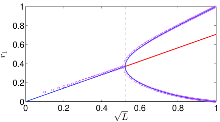
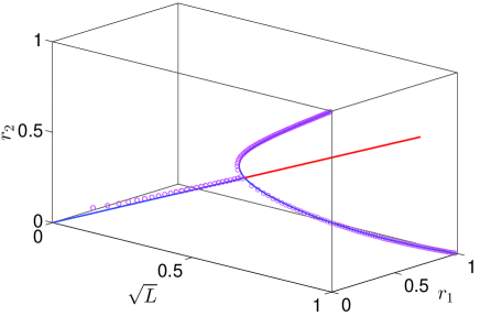
Figure 1: (Color online). Bifurcation scenario for $N=2$ same charge vortices and corresponding MC simulations. The bifurcation diagram, as a function of the square root of the angular momentum of the system ($\sqrt{L}$) is increased, obtained from the corresponding ODEs (1) is depicted by the solid lines where blue denotes a stable branch and red an unstable branch. The MC simulation results are depicted with the small magenta circles. The critical point beyond which (through a supercritical pitchfork bifurcation) the asymmetric configurations arise –and become a ground state of the system– is indicated by the vertical dashed line. Note how the MC simulations nicely follow the stable branches of the bifurcation diagram.

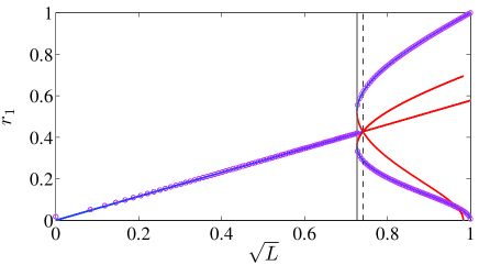
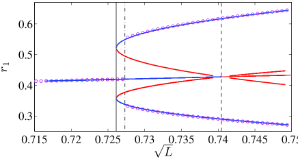
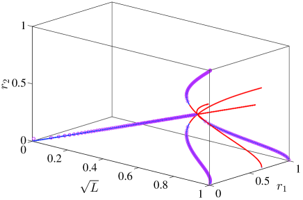
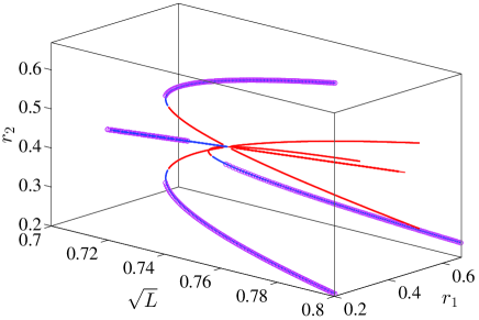
Figure 2: (Color online). Bifurcation scenario for $N=3$ same charge vortices and corresponding MC simulations. Same notation as in Fig. 1. The left panels correspond to the entire domain $0\leq L\leq 1$ while the right panels depict a zoomed in version near the bifurcation region. The top panels show the bifurcation diagrams in a planar view, namely $r_{i}$ vs. $\sqrt{L}$. The bottom panels depict the bifurcation diagram in the three dimensional space ($\sqrt{L},r_{1},r_{2}$) where the the $C_{3}$ symmetry of the solution is clearly visible. The thin dashed vertical line corresponds to the symmetry breaking bifurcation where the symmetric (equilateral triangle) loses its stability. The thin solid vertical line depicts the location of the saddle-center bifurcation of collisions between asymmetric (isosceles triangle) solutions. The thin dash-dotted vertical line corresponds to the location where the MC simulation switches branches (i.e., location where the energy minimum configuration switches from an equilateral to an isosceles one).

IV Results

We now present our results in terms of the (numerically) exact bifurcation diagrams of the coupled systems of ODEs (1) and the corresponding approximate (ground state) phase diagrams obtained by the MC methodology described in the previous section. We will perform this comparison for $N=2,3$, and $4$ vortices and present the MC results for $N=5$ vortices. In all of these cases, we complement our computations with analytical results, wherever possible.

IV.1 The N=2 Vortex Case

We start by examining for completeness (and in order to set the stage for follow-up observations) the case of $N=2$ that was previously considered in some detail in Ref. corot_prl . As discussed in that work, for values of the angular momentum $L<L_{cr}^{(2)}\equiv 2\sqrt{c}/(\sqrt{c}+2)$, i.e., for radial displacements of the vortices $r<r_{cr}^{(2)}\equiv\sqrt{\sqrt{c}/(\sqrt{c}+2)}$, the symmetric rigidly rotating vortex state, namely two vortices at equal distances from the center of the trap, is stable. However, for radii (or angular momenta) above this critical point, the symmetric state becomes structurally unstable and gives rise, through a super-critical, for the range of $c$’s of relevance to the experiment, pitchfork bifurcation (i.e., a spontaneous symmetry breaking), to the emergence of asymmetric, yet still anti-diametric, rigidly rotating states. In the latter, one of the vortices is always further away from the origin, say $r_{1}$, while the other is closer, say $r_{2}$ ($r_{2}<r_{1}$), such that the angular momentum constraint $L=r_{1}^{2}+r_{2}^{2}$ is satisfied and also

$$-r_{1}r_{2}(r_{1}+r_{2})^{2}+c(1-r_{1}^{2})(1-r_{2}^{2})=0.$$ (7)

This analytical expression identified in Ref. corot_prl by means of a direct solution of the equations of motion, along with the angular momentum constraint and the necessity that $\delta_{12}=\pi$ (i.e., anti-diametric vortices) fully characterize the class of asymmetric solutions in the case of $N=2$.

Our Monte-Carlo analysis does an excellent job of capturing the relevant minimizers of the energy. As it is clear from the (magenta) data points of Fig. 1, up to the critical point $L_{cr}^{(2)}$ (see vertical dashed line), the Monte-Carlo computation follows the symmetric branch (see blue line for $L<L_{cr}^{(2)}$), while past the critical point, it follows the newly emergent and stable (see blue curves for $L>L_{cr}^{(2)}$) asymmetric branch arising from the pitchfork bifurcation. This case serves as a useful benchmark between the analysis and the numerical MC computation, and as a prototypical example of the phenomenology that will follow, involving the spontaneous emergence of asymmetric rigidly rotating states and which will be progressively more complex as the number of vortices $N$ increases.

IV.2 The N=3 Vortex Case

For $N=3$, the symmetric rigidly rotating solution naturally persists (in fact, it persists for all the $N$’s that we have considered) with the relevant inter-vortex angle being $\delta_{ij}=2\pi/N=2\pi/3$ in this case. The angular momentum constraint for this equilateral solution reads $L=Nr^{2}=3r^{2}$. The stability of this solution can be also identified analytically. In particular, there is an eigenfrequency associated with it assuming the analytical form:

$$\omega^{2}=\frac{c^{2}}{r^{4}}-\frac{2c}{(1-r^{2})^{2}}.$$ (8)

The zero crossing of this squared eigenfrequency at $r=r_{cr}^{(3)}\equiv\sqrt{{\sqrt{c}}/({\sqrt{c}+\sqrt{2}})}=0.4275$ yields the destabilization point of the equilateral triangle. The corresponding critical angular momentum satisfies: $\sqrt{L_{cr,1}^{(3)}}=\sqrt{3}r_{cr}^{(3)}=0.7404$. This critical threshold is depicted by the thin vertical dashed line in Fig. 2 (and also Fig. 3).

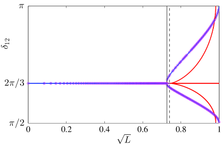
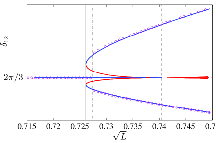
Figure 3: (Color online). Bifurcation scenario for the relative angles between vortices $\delta_{12}$ as a function of the (square root) of the angular momentum for $N=3$ vortices. The data is the same as Fig. 2 and the notation is also the same. The top panel is the full view while the bottom panel depicts a zoomed in version around the bifurcation region.

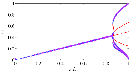
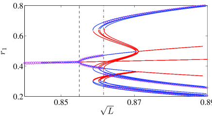
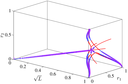
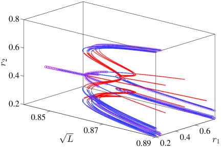
Figure 4: (Color online). Bifurcation scenario and corresponding MC simulations showing the complete dynamical picture associated with the transitions/instabilities in the case of $N=4$. Similarly to the $N=3$ case, the top panels show a planar representation of the solutions using only $r_{1}$ as a function of $\sqrt{L}$, while the bottom panels relay a 3-dimensional variant thereof with $r_{2}$, as a function of $r_{1}$ and $\sqrt{L}$. The blue lines are stable branches, while the red lines represent the unstable branches and the Monte-Carlo data are overlayed using small magenta circles. This conveys, not only how new branches (such as the rhombus and general quadrilateral) emerge through suitable bifurcations (supercritical pitchfork or saddle-center, respectively), but also when they become the global energy minimizers and hence are followed by the Monte-Carlo simulation. Specifically, the thin dashed vertical line corresponds to the symmetry breaking bifurcation where the symmetric (square) configuration loses its stability towards the newly created rhombus configuration, while the thin dash-dotted vertical line corresponds to the location where the MC simulation switches branches (i.e., transitions from the rhombic configuration to a more general quadrilateral without any apparent symmetry).

The $N=3$ case is richer than $N=2$. In particular, in addition to the symmetry-breaking pitchfork bifurcation that destabilizes the symmetric (equilateral triangle) solutions, which is equivalent to the one we described for the $N=2$ case, there is another bifurcation. This secondary bifurcation happens at the critical point $L_{cr,2}^{(3)}$ where new solutions emerge (see threshold depicted by the thin solid vertical line in Fig. 2). In fact, this is a pair of solutions with a trilateral symmetry ($C_{3}$) corresponding to the three possible isosceles triangles of vortices that can emerge as rigidly rotating solutions in the system. For these solutions, one of the vortices is at, say a longer distance from the origin, $r_{1}$, while the other two are at, say a shorter distance $r_{2}$. Then the angular momentum constraint reads $L=r_{1}^{2}+2r_{2}^{2}$, while the following conditions completely specify the relevant solution in an analytical form:

$$\delta_{12} = \delta_{31}=\frac{d\pm\sqrt{d^{2}+8}}{4},$$

$$\delta_{23} = 2\pi-2\delta_{12},$$ (9)

$$c = \frac{3r_{1}^{4}r_{2}^{2}+3r_{1}^{2}r_{2}^{4}-a\,r_{1}^{3}r_{2}^{3}}{(1-r_{1}^{2})(1-r_{2}^{2})(r_{1}^{2}-r_{2}^{2}-a\,r_{1}r_{2})}$$

where $\cos(d)\equiv(r_{1}^{2}+r_{2}^{2})/(2r_{1}r_{2})$, and $a^{2}\equiv{r_{1}^{4}+34r_{1}^{2}r_{2}^{2}+r_{2}^{4}}$.

While we have attempted to identify this secondary critical point in a tractable analytical form, it has not been possible given the complexity of the above solution. Nevertheless, we have been able to identify numerically that the relevant bifurcation that leads to the emergence of the isosceles triangles is a saddle-center one. Namely, each of the 3 (rotated by 120${}^{\,0}\deg$) triangles comes with an “unstable partner”. This saddle-center bifurcation arises numerically at $L_{cr,2}^{(3)}=0.527\Rightarrow\sqrt{L_{cr,2}^{(3)}}=0.726$, as illustrated by the thin solid vertical line in Fig. 2. It is in fact very close to this point that the Monte-Carlo computation will jump at this newly arising (stable such) branch. That is to say, almost as soon as the branch is born, it becomes the global minimum of the energy surface. Remarkably, it is the unstable partner of these isosceles saddle-center pairs which collides with the symmetric, equilateral solution at $L_{cr,1}^{(3)}=0.548\Rightarrow\sqrt{L_{cr,1}^{(3)}}=0.7404$ (see threshold depicted by a thin dashed vertical line in Fig. 2). Our dynamical and eigenvalue computations of Fig. 2 capture this transition but the Monte-Carlo is entirely insensitive to this step. This, in turn, suggests the relevance of the Monte-Carlo as a convenient tool for identifying the global energy minimum of the system but also the usefulness of the full dynamical systems analysis provided herein as a means of identifying metastable states and transitions between them. The combination of the two unveils some of the complexities of the full energy surface. While Fig. 2 focuses on the dependence of the radii of the particles as a function of the angular momentum $L$, Fig. 3 shows the corresponding relative angles between vortices ($\delta_{ij}$). These deviate from their equilateral value of $2\pi/3$ in an asymmetric manner, revealing the isosceles character of the triangle given that out of the three equal angles, only two remain equal while the third acquires a different value.

IV.3 The N=4 Vortex Case

We now turn to the more complex case of $N=4$. Here, too, the symmetric solution exists with $L=4r^{2}$ and $\delta_{ij}=\pi/2$. However, the linearization around it now features two internal modes. The first of them has the frequency

$$\omega_{1}^{2}=\frac{2c^{2}}{r^{4}}-\frac{4c}{(1-r^{2})^{2}},$$ (10)

and remarkably crosses zero (and thus marks the critical point for the destabilization of the configuration) at the same point as the $N=3$ case, i.e., at $r=r_{cr,1}^{(4)}\equiv\sqrt{{\sqrt{c}}/(\sqrt{c}+\sqrt{2})}$, which, however, now corresponds to the higher angular momentum $L_{cr,1}^{(4)}=4{\sqrt{c}}/({\sqrt{c}+\sqrt{2}})$. The second of these critical points corresponds to the eigenfrequency:

$$\omega_{2}^{2}=\frac{9c^{2}}{4r^{4}}-\frac{3c}{(1-r^{2})^{2}}$$ (11)

which vanishes at $r^{2}=(r_{cr,2}^{(4)})^{2}\equiv{\sqrt{3c}}/({\sqrt{3c}+2})$; this second critical point does not appear to be of particular interest to our study here.

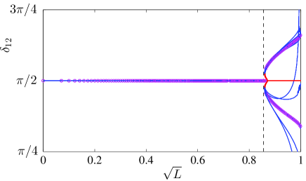
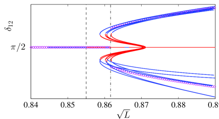
Figure 5: (Color online). Bifurcation scenario for the relative angles between vortices $\delta_{12}$ as a function of the (square root) of the angular momentum for $N=4$ vortices. The data is the same as Fig. 4 and the notation is also the same. The top panel is the full view while the bottom panel depicts a zoomed in version around the bifurcation region. Notice that between the transition from the square to the rhombus (dashed vertical line) and that from the rhombus to the general quadrilateral (dash-dotted vertical line), no modification is noticed by looking solely at the angles, as the rhombic configuration maintains $\delta_{12}=\pi/2$.

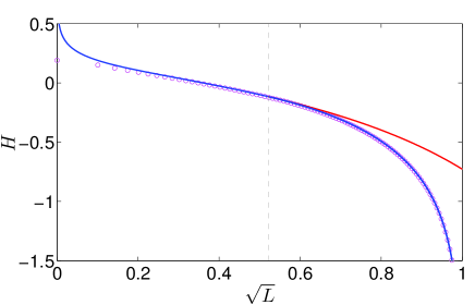
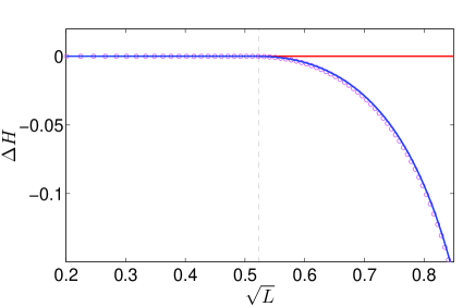
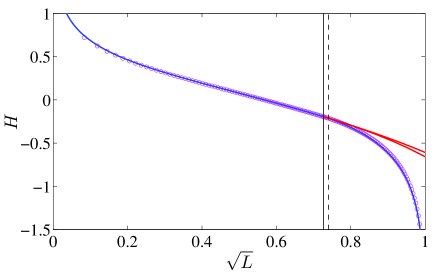
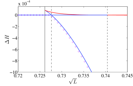
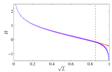
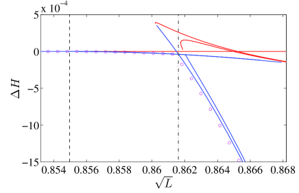
Figure 6: (Color online). Energy corresponding to all the bifurcation branches presented in the previous plots together with the energy computed from the MC simulations. As before, the bifurcation branches are depicted by a blue (red) line for stable (unstable) branches and the MC simulations are depicted with the magenta circles. The first, second and third rows of panels correspond, respectively, to the $N=2$, $3$ and $4$ cases. The left panels present the energy as computed from Eq. (3) over the entire range $0\leq L\leq 1$, while the right panels depict the corresponding energy difference $\Delta H$ between each configuration and the corresponding symmetric configuration for each value of $L$ (see text for more details).

In addition to the square configuration, we have again sought the possibility of unveiling analytically reduced symmetry solutions. An example that we have been able to identify in this case is a rhombic configuration with $r_{1}=r_{3}$ and $r_{2}=r_{4}$ in which case still all the $\delta_{ij}=\pi/2$. For this configuration we have been able to find that it consists of two longer and two shorter segments $r_{1}$ and $r_{2}$ such that $L=2(r_{1}^{2}+r_{2}^{2})$ and $r_{2}=\sqrt{c(1-r_{1}^{2})/(2r_{1}^{2}+c(r_{1}^{2}-1))}$. It is then straightforward to observe that this configuration “collides” with the square branch (i.e., $r_{2}=r_{1}$) exactly at $r=r_{cr,1}^{(4)}$ which is precisely where the square configuration loses its stability through the zero-crossing of the frequency $\omega_{1}$. From the above and since this solution exists only above this critical point, it can be inferred that the primary instability of the square configuration leads to a supercritical pitchfork bifurcation that, in turn, results in the emergence of the rhombic state. This is confirmed in Fig. 4 where the location of this primary bifurcation indeed occurs at $r_{cr,1}^{(4)}$, see dashed vertical line.

Numerically, we indeed observe this destabilization and the corresponding symmetry breaking bifurcation which is depicted in Fig. 4. In particular, a destabilization event for $c=0.1$ clearly arises at $\sqrt{L}=0.862$ in the Monte-Carlo (see vertical dash-dotted line), while the corresponding analytical prediction is at $(L_{cr,1}^{(4)})^{1/2}=0.855$ (see vertical dashed line). It is particularly interesting that close inspection of Fig. 4 reveals for a few points between $0.855$ and $0.862$ the transition from the square to the rhombi (although the growth rate of the associated instability in this interval is apparently so weak that the MC may still converge to the squares for some values of $\sqrt{L}$ within this interval). On the other hand, we also depict the relevant bifurcation for the relative angles $\delta_{ij}$ in Fig. 5. Remarkably but also naturally, between $0.855$ and $0.862$, and while the radii reveal (at least partially) the transition from the squares to the rhombi, $\delta_{12}$ remains invariant at $\pi/2$, as it is shared by both configurations. Hence, it is clear that one cannot use solely the radii or solely the relative angles, but a careful inspection of both unveils the full picture of configurational transitions. For slightly higher values of the angular momentum, i.e., for $\sqrt{L}>0.8626$, the Monte-Carlo jumps to another configuration which in this case does not appear to have any definite symmetry. While the relative angles $\delta_{ij}$, as discussed above, were unable to “discern” the first transition (the supercritical pitchfork from the square to the rhombus), nevertheless, they clearly distinguish the second transition, whereafter none of the angles is equal to $\pi/2$.

It should be clear at this point that, as in the $N=3$ case, in the $N=4$ examples as well, the dynamical picture offers a particularly useful complementing view which corroborates in an insightful manner the results of the Monte-Carlo approach. In particular, we clearly observe the transition from the square to the rhombus. The latter state, however, is apparently the ground state of the $N=4$ system only for a small interval of angular momenta. This is because already for $\sqrt{L}=0.859$ a pair of asymmetric (so-called irregular) quadrilaterals of vortices arise with unequal sides, yet rigidly rotating around the center of the trap. Remarkably, one of the highly asymmetric configurations that arise in this saddle-center bifurcation is dynamically stable and it is that one that becomes the global energy minimum beyond the second critical point, namely $\sqrt{L}=0.8626$. For these quadrilaterals it can be seen that approximately $r_{1}=r_{3}$, $r_{2}$ is close to $r_{1},r_{3}$ but clearly not equal and $r_{4}$ much larger (rotated versions of such quadrilaterals also obviously exist from symmetry). Interestingly, the dynamical picture reveals one more feature, namely that such quadrilaterals collide via a sub-critical pitchfork with the rhombic configuration for $L^{1/2}=0.87$. I.e., the full dynamics and stability picture is far more complicated, involving a series of bifurcations, a super-critical and a sub-critical pitchfork, as well as a saddle-center bifurcation, yet again the combination of the Monte-Carlo method and the bifurcation analysis yields a complete understanding of the system’s ground state features.

Finally, in order to more precisely illustrate the feature that the MC simulation is indeed converging to the stable state with minimum energy, we have followed the Hamiltonian (3) as the angular momentum is varied. The results for $N=2$, $3$ and $4$ are depicted in Fig. 6. The left column on the panels corresponds to the total energy as given by Eq. (3), while the right panels depict zoomed in versions for the energy difference $\Delta H$ between the configuration at hand and the symmetric state. Namely, we define $\Delta H=H-H_{0}$, where $H$ is computed using Eq. (3) for each configuration and $H_{0}=H(r_{i}=r^{*},\delta_{i,i\pm 1}=\delta^{*})$ where $(r^{*},\delta^{*})$ correspond to the radius and relative angle for a symmetric polygonal configuration. Namely, for $N$ vortices these correspond to $r^{*}=\sqrt{L/N}$ and $\delta^{*}=2\pi/N$. In the case of $N=2$, the picture is very clear: as soon as the asymmetric anti-diametric configuration emerges, the MC converges to it. For $N=3$, the emergence of the asymmetric isosceles states occurs well before the destabilization of the equilateral, co-rotating triangle branch. Nevertheless, very shortly after the saddle-center bifurcation of this new branch (cf. the vertical solid with the vertical dash-dotted line in the middle right panel Fig. 6), the MC jumps to the newly emergent, asymmetric branch as soon as the latter becomes energetically favorable, yet well before the instability of the equilateral branch (occurring at the location of the vertical dashed line). The case of $N=4$ is more complex. Here we can see that once the square configuration destabilizes towards the rhombic one (vertical dashed line), the MC follows the rhombi until very shortly after the emergence of the irregular quadrilateral branch; the latter, is generated by the saddle-center bifurcation, and acquires lower energy than the rhombi (vertical dash-dotted line). Immediately thereafter, the MC approach traces this and jumps to it. It is clear from the results presented in Fig. 6 that the MC simulations indeed converge, for a given $L$ to the stable state which has the lowest energy among the different vortex configurations.

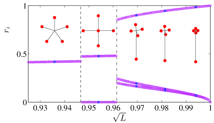
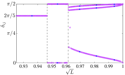
Figure 7: (Color online) Monte-Carlo results for $N=5$ vortices. The top and bottom panel depict, respectively, the MC results for the radii ($r_{i}$) and the relative angles ($\delta_{ij}$). Two transitions are observed. The first transition at $L^{1/2}=0.9467$ (location depicted by the vertical dashed line) indicates where the configuration with a single vortex at the center turns into the ground state of the system. The second transition observed at $L^{1/2}=0.9615$ (location depicted by the vertical dash-dotted line) indicates where the asymmetric configuration (a tight cluster of 4 vortices plus a single vortex further away from the center) turns into the ground state of the system. The filled (blue) dots along the different branches indicate the locations of the displayed vortex configurations in the top panel.

IV.4 The N=5 Vortex Case

For the case of $N=5$, the relevant calculations both analytical and numerical become, arguably, very complex. Nevertheless, we have still been able to analyze the stability of the pentagon configuration with $r=r_{i}$, $L=5r^{2}$ and $\delta_{ij}=2\pi/5$. Such configurations will be stable, remarkably, until the same principal critical point as were $N=3$ and $N=4$ polygons, namely $r^{2}=(r_{cr,1}^{(5)})^{2}\equiv{\sqrt{c}}/({\sqrt{c}+\sqrt{2}})$, although, of course this corresponds to a higher angular momentum for this case, namely $L_{cr,1}^{(5)}=5(r_{cr,1}^{(5)})^{2}$. On the other hand, we have also been able to identify a second critical point which arises at $r^{2}=(r_{cr,2}^{(5)})^{2}\equiv{\sqrt{c}}/({\sqrt{c}+1})$, i.e., at a higher radius. This first critical point occurs analytically at $\sqrt{L}=0.956$, while the Monte-Carlo numerically appears to deviate from the pentagon configuration for the earlier value of $\sqrt{L}=0.9467$. However, as is clear from the Monte-Carlo results of Fig. 7, the bifurcation occurring at this point cannot be a supercritical pitchfork one, given the sizeable “jump” of the values of the $r_{i}$’s occurring at this point. Under close inspection, this first transition captured by the MC simulations corresponds to a value for the angular momentum where another, independent configuration branch becomes the ground state of the system. In fact, apparently, for values of the angular momentum in $0.9467<L^{1/2}<0.9615$, the configuration bearing a single vortex at the center surrounded by a square of vortices has less energy than the pentagon. For larger values of the angular momentum, $L^{1/2}>0.9615$, the asymmetric configuration bearing a tight cluster of four vortices near the origin and a single vortex further away from the center, corresponds to the lowest energy configuration of the system. Identifying the conditions for the existence of windows where the configuration with a single vortex at the center with a polygon of $N-1$ vortices around it is more energetically favorable than a polygon of $N$ vortices remains an interesting open problem for future work.

V Conclusions and Future Work

In the present work, we have used a combination of analytical and numerical techniques to shed light on the (already fairly complex for small number of vortices) possible solutions and associated bifurcations of co-rotating vortices in atomic Bose-Einstein condensates. Building on the earlier establishment of a relevant model through comparisons with experimental results, e.g., in Refs. middel_pra11 ; corot_prl , we developed both a Monte-Carlo approach targeting the lowest energy states and an AUTO-based dynamical systems approach attempting to infer the relevant solutions and their pitchfork and saddle-center bifurcations into existence/termination. By corroborating the two techniques and using the angular momentum as a parameter, and the energy as well as the vortex positions as diagnostics, we were able to provide a full picture of how two rigidly rotating vortices remain anti-diametric but become asymmetric, three rigidly rotating vortices prefer to be in an isosceles rather than equilateral triangle, while four turn from squares to rhombi and from there to irregular quadrilaterals. All these transitions have been quantified as a function of increasing angular momenta and ultimately result from the competition of the two energetic contributions in Eq. (3), namely the precession of each vortex due to the trap and the pairwise interaction between the vortices. Whenever possible the numerical observations have been complemented by analytical solutions (e.g. identifying the destabilization points of symmetric configurations, or analytically characterizing the bifurcating solutions such as isosceles triangles and rhombi).

Nevertheless, naturally many open questions still remain and the system clearly merits further investigation. As an appetizer towards that direction, we presented the calculation of $N=5$, indicating a clearly subcritical event that must be leading to the destabilization of the pentagons. Our computational approaches have natural limitations that arise both for the dynamical systems AUTO-based analysis and for the Monte-Carlo efficient ground state tracking method. We now briefly discuss these limitations and present a view towards overcoming them in the future which would indeed enable a systematic categorization of larger vortex particle clouds.

On the one hand, the AUTO calculation is extremely useful in identifying the relevant bifurcations, but given that it tracks the different branches of solutions, it provides a progressively more complex and difficult to parse picture as $N$ is increased. Hence, it is necessary to use multiple and different suitably chosen diagnostics in order to be able to systematically scale up the picture to cases of larger $N$. It would be particularly meaningful of a task to try to develop such diagnostics and it is part of our currently ongoing effort. On the other hand, the Monte-Carlo approach suffers from a different limitation most notably the divergence of vortex precessional frequencies (and logarithmic associated single vortex energy contributions) when $r_{i}\rightarrow 1$. It is precisely for that reason that we have confined our consideration on the MC side to $L<1$. It naturally turns out that when $L\geq 1$, the energy minimization can be trivially (but meaninglessly, as far as the physical problem is concerned) be realized by means of one (or more) of the $r_{i}\rightarrow 1$ and hence $H\rightarrow-\infty$. Hence, it is of paramount importance in that regard to amend the “pathological” precessional frequency expression with one that more accurately predicts the $r\rightarrow 1$ regime in comparison to the partial differential equation (PDE) (see also the relevant partial disparity in Fig. 1a of Ref. corot_prl , for vortices at distances very proximal to the TF radius). A combination of variants of the above tools devoid of these technical limitations (for small and intermediate $N$) and possible intriguing tools from PDE theory about vortex “densities” (for large $N$) in the spirit e.g. of the recent work of Ref. theo can provide valuable insights for future studies of vortices, but also of other types of solitonic populations, such as dark solitons in 1D or vortex rings in 3D BECs ourexpo . Such studies are currently in progress and will be reported in future publications.

Finally, it is important to note that the results we present in this manuscript are based on the assumption of an axially symmetric trapping potential. If one relaxes this symmetry and considers different trapping strengths along the longitudinal directions, the vortex precession rate has to be adjusted and depends on the angular position of the vortex with respect to the trapping axes Fetter_Svidzinsky_2000 ; see also Ref. middel_anis for multi-vortex settings. The dynamics for asymmetric trapping is much richer than the one presented here and will be showcased in a future publication.

- (1) C.J. Pethick and H. Smith, Bose-Einstein condensation in dilute gases, Cambridge University Press (Cambridge, 2002).
- (2) L.P. Pitaevskii and S. Stringari, Bose-Einstein Condensation, Oxford University Press (Oxford, 2003).
- (3) P.G. Kevrekidis, D.J. Frantzeskakis, and R. Carretero-González, Emergent Nonlinear Phenomena in Bose-Einstein Condensates, Springer-Verlag, Berlin, 2008.
- (4) R.J. Donnelly, Quantized Vortices in Helium II, Cambridge University Press, New York, 1991;
- (5) A.L. Fetter and A.A. Svidzinsky, J. Phys.: Condens. Matter 13, R135 (2001).
- (6) A.L. Fetter, Rev. Mod. Phys. 81, 647 (2009).
- (7) P.G. Kevrekidis, R. Carretero-González, D.J. Frantzeskakis, and I.G. Kevrekidis, Mod. Phys. Lett. B 18, 1481 (2004).
- (8) M. Tsubota, K. Kasamatsu, and M. Kobayashi, arXiv:1004.5458.
- (9) B.P. Anderson, J. Low Temp. Phys. 161, 574 (2010).
- (10) A.E. Leanhardt, A. Görlitz, A.P. Chikkatur, D. Kielpinski, Y. Shin, D.E. Pritchard, and W. Ketterle, Phys. Rev. Lett. 89, 190403 (2002); Y. Shin, M. Saba, M. Vengalattore, T.A. Pasquini, C. Sanner, A.E. Leanhardt, M. Prentiss, D.E. Pritchard, and W. Ketterle, Phys. Rev. Lett. 93, 160406 (2004).
- (11) C. Raman, J.R. Abo-Shaeer, J.M. Vogels, K. Xu, and W. Ketterle, Phys. Rev. Lett. 87, 210402 (2001).
- (12) C. Weiler, T. Neely, D. Scherer, A. Bradley, M. Davis, and B.P. Anderson, Nature 455, 948 (2008).
- (13) D.V. Freilich, D.M. Bianchi, A.M. Kaufman, T.K. Langin, and D.S. Hall, Science 329, 1182 (2010).
- (14) T.W. Neely, E.C. Samson, A.S. Bradley, M.J. Davis, and B.P. Anderson, Phys. Rev. Lett. 104, 160401 (2010).
- (15) S. Middelkamp, P. J. Torres, P. G. Kevrekidis, D. J. Frantzeskakis, R. Carretero-González, P. Schmelcher, D. V. Freilich, and D. S. Hall, Phys. Rev. A 84, 011605 (2011).
- (16) R. Navarro, R. Carretero-González, P.J. Torres, P.G. Kevrekidis, D.J. Frantzeskakis, M.W. Ray, E. Altuntas and D.S. Hall, Phys. Rev. Lett. 110, 225301 (2013).
- (17) J.A. Seman, E.A.L. Henn, M. Haque, R.F. Shiozaki, E.R.F. Ramos, M. Caracanhas, P. Castilho, C. Castelo Branco, P.E.S. Tavares, F.J. Poveda-Cuevas, G. Roati, K.M.F. Magalhães, and V.S. Bagnato, Phys. Rev. A 82, 033616 (2010).
- (18) K.W. Madison, F. Chevy, W. Wohlleben, and J. Dalibard, Phys. Rev. Lett. 84 806 (2000).
- (19) Y. Castin, R. Dum, Eur. Phys. J. D 7, 399 (1999).
- (20) L.-C. Crasovan, V. Vekslerchik, V.M. Pérez-García, J.P. Torres, D. Mihalache, and L. Torner, Phys. Rev. A 68 063609 (2003).
- (21) M. Möttönen, S.M.M. Virtanen, T. Isoshima, and M.M. Salomaa, Phys. Rev. A 71, 033626 (2005).
- (22) V. Pietilä, M. Möttönen, T. Isoshima, J.A.M. Huhtamäki, and S.M.M. Virtanen, Phys. Rev. A 74, 023603 (2006).
- (23) L.C. Crasovan, G. Molina-Terriza, J.P. Torres, Ll. Torner, V.M. Pérez-García, and D. Mihalache, Phys. Rev. E 66, 036612 (2002).
- (24) G. Molina-Terriza, Ll. Torner, E.M. Wright, J.J. García-Ripoll, and V.M. Pérez-García, Opt. Lett. 26 1601 (2001).
- (25) A. Klein, D. Jaksch, Y. Zhang, and W. Bao, Phys. Rev. A 76, 043602 (2007).
- (26) W. Li, M. Haque, and S. Komineas, Phys. Rev. A 77, 053610 (2008).
- (27) J. Brand and W.P. Reinhardt, Phys. Rev. A 65, 043612 (2002).
- (28) S. Middelkamp, P.G. Kevrekidis, D.J. Frantzeskakis, R. Carretero-González, and P. Schmelcher, Phys. Rev. A 82, 013646 (2010).
- (29) P. Kuopanportti, J.A.M. Huhtamäki, and M. Möttönen, Phys. Rev. A 83, 011603(R) (2011).
- (30) S. Middelkamp, P.G. Kevrekidis, D.J. Frantzeskakis, R. Carretero-González, and P. Schmelcher, Phys. D 240, 1449 (2011).
- (31) P.J. Torres, P. G. Kevrekidis, D. J. Frantzeskakis, R. Carretero-González, P. Schmelcher, and D. S. Hall, Phys. Lett. A 375, 3044 (2011).
- (32) J. Stockhofe, S. Middelkamp, P. G. Kevrekidis, and P. Schmelcher, EPL 93, 20008 (2011).
- (33) http://indy.cs.concordia.ca/auto/
- (34) S.-M. Chang, W.-W. Lin, and T.-C. Lin, Int. J. Bif. Chaos 12, 739 (2002).
- (35) D.E. Pelinovsky and P.G. Kevrekidis, Nonlinearity 24, 1271 (2011).
- (36) S.W.S. Apolinario, B. Partoens, and F.M. Peeters, Phys. Rev. E 72, 046122 (2005).
- (37) M. Saint Jean and C Guthmann, J. Phys: Condens. Matter 14, 13653 (2002).
- (38) Y. Chen, T. Kolokolnikov, and D. Zhirov, Proceedings of the Royal Society A 469, 20130085 (2013).
- (39) See, e.g., for an overview discussion encompassing the different structures: Dynamical Systems Magazine, October 2011, P.G. Kevrekidis, R. Carretero-González, and D.J. Frantzeskakis. “Vortices in Bose-Einstein Condensates: (Super)fluids with a twist”. URL: http://www.dynamicalsystems.org/ma/ma/display?item=397
- (40) A.A. Svidzinsky and A.L. Fetter, Phys. Rev. Lett. 84, 5919 (2000).