$(N+1)$-dimensional Lorentzian evolving wormholes supported by polytropic matter

Abstract: In this paper we study $(N+1)$-dimensional evolving wormholes supported by energy satisfying a polytropic equation of state. The considered evolving wormhole models are described by a constant redshift function and generalizes the standard flat Friedmann-Robertson-Walker spacetime. The polytropic equation of state allows us to consider in $(3+1)$-dimensions generalizations of the phantom energy and the generalized Chaplygin gas sources.

I Introduction

Wormholes are exotic solutions of Einstein’s field equations representing tunnels through space-time connecting two different regions of our Universe or even another Universe. The focus of studying wormhole geometries has intensively increased since the publication of works of Morris and Thorne 1 ; 1A ; Visser , where it was proposed the possibility of the existence of traversable wormholes allowing to travel through space and time. The idea of such a travel always has been interesting for the humanity so a lot of works has studied wormhole models with different types of matter supporting them StaticWH ; StaticWHA ; StaticWHB ; StaticWHC ; StaticWHD ; StaticWHE ; StaticWHF ; StaticWHG ; StaticWHH ; StaticWHI ; StaticWHJ ; StaticWHK ; StaticWHL ; StaticWHM ; StaticWHN ; StaticWHO , or in alternative theories of gravity Alternative ; AlternativeA ; AlternativeB ; AlternativeC . Most considered models are stationary spherically symmetric wormholes. The matter responsible for sustaining a traversable wormhole is exotic since it violates the standard null and weak energy conditions. In other words, it would only be possible to cross such a stationary wormhole if exotic matter with negative energy density sustain it. Constructed static spherically symmetric wormholes are described by the metric 1 ; Visser

$$ds^{2} = -e^{\Phi(r)}dt^{2}+\frac{dr^{2}}{1-\frac{b(r)}{r}}+d\Omega^{2},$$ (1)

where $\Phi(r)$ is the redshift function and $b(r)$ the shape function. These functions depend on the form assumed for the energy-momentum tensor coupled to the metric  (1). In order to have a wormhole geometry the redshift and shape functions must obey some specific conditions such as for example $\Phi(r)$ must be finite everywhere for guaranteeing the absence of horizons and singularities in the space-time, $b(r=r_{0})=r_{0}$ at a throat, $b(r)/r\leq 1$ and, in order to have an asymptotically Minkowskian space-time, the condition $b(r)/r\rightarrow 0$ at $r\rightarrow\infty$ must be required.

This wormhole concept can be extended to time-dependent wormhole geometries. The metric considered for describing such an evolving wormhole may be written in the form

$$ds^{2} = -e^{-2\Phi(t,r)}dt^{2}+a^{2}(t)\left[\frac{dr^{2}}{1-\frac{b(r)}{r}}+r^{2}d\Omega^{2}\right],$$ (2)

where the redshift function now depends on the time and radial coordinates, and the new function $a(t)$ is the scale factor. This function controls the expansion of the wormhole, and its evolution is dictated by Einstein’s field equations.

In this paper we want to discuss wormhole models supported by polytropic phantom energy, resulting in an extension of the polytropic wormholes discussed in Ref. jamil . The generalization goes in two ways. First, we are interested in obtaining a static $(N+1)$-dimensional extension of zero-tidal-force wormhole models studied in Ref. jamil . The second extension consists in their dynamic generalization by introducing a scale factor with the help of the metric (2).

It must be noticed, for example, that in four dimensional spherically symmetric spacetimes analytical solutions for polytropic star configurations are known just for a few particular values of the polytropic index (excluding the linear equation of state $p=\omega\rho$). An interesting discussion involving polytropic equations of state for general relativistic stars is given in Ref. Nilsson . In Ref. 4 , authors found solutions for a compressible polytropic fluid sphere in gravitational equilibrium. A study on polytropic stars in three-dimensional space-time is made in Sa . It therefore seems of interest to find spherically symmetric gravitational models supported with matter fields obeying a polytropic equation of state.

The organization of the paper is as follows: In Sec. II we present the dynamical field equations for wormhole models with a matter source obeying a polytropic equation of state. In Sec. III solutions to these field equations are studied, and in Sec. IV we conclude with some remarks.

II $(N+1)$-dimensional evolving wormholes

Let us now consider the $(N+1)$-dimensional extension of the metric (2), with a vanishing redshift function, described in comoving coordinates $(t,r,\theta_{1},...\theta_{N-1})$ by the metric

$$ds^{2} = -dt^{2}+a^{2}(t)\left[\frac{dr^{2}}{1-\frac{b(r)}{r}}+r^{2}d\Omega^{2}_{N-1}\right],\,\,\,\,\,\,\,$$ (3)

where $d\Omega^{2}_{N-1}$ is the metric on a $(N-1)$ sphere. Since $\Phi(t,r)=0$ this metric describes a zero-tidal-force wormholes, ensuring the absence of horizons and singularities in the considered space-time. It is clear that the metric (3) becomes an $(N+1)$-dimensional static zero-tidal-force wormhole if $a(t)\rightarrow\textrm{constant}$ and, as $b(r)\rightarrow 0$, it becomes a flat $(N+1)$-dimensional extension of the Friedmann-Robertson-Walker (FRW) metric.

In order to simplify the analysis we shall rewrite the metric as

$$ds^{2} = -\theta^{(t)}\theta^{(t)}+\theta^{(r)}\theta^{(r)}+\sum_{i=1}^{N-1}{\theta^{(\theta_{i})}\theta^{(\theta_{i})}},$$ (4)

where the following $(N+1)$-dimensional proper orthonormal basis of one-forms

$$\theta^{(t)} = dt,$$ (5)

$$\theta^{(r)} = a(t)\frac{dr}{\sqrt{1-\frac{b(r)}{r}}},$$ (6)

$$\theta^{(\theta_{1})} = a(t)rd_{\theta_{1}},$$ (7)

$$\theta^{(\theta_{2})} = a(t)r\sin{\theta_{1}}d_{\theta_{2}},$$ (8)

$$\theta^{(\theta_{N-1})} = a(t)r\prod_{i=1}^{N-2}{\sin{\theta_{i}}d\theta_{N-1}},$$ (9)

has been introduced. We shall consider a matter source described by an inhomogeneous and anisotropic fluid with a diagonal energy-momentum tensor. Then the only nonzero components of the energy-momentum tensor in the basis (5)-(9) are:

$$T_{(t)(t)} = \rho(t,r),$$ (10)

$$T_{(r)(r)} = p_{r}(t,r),$$ (11)

$$T_{(\theta)(\theta)} =...= T_{(\theta_{N-1})(\theta_{N-1})}=p_{l}(t,r),$$ (12)

where $p_{r}(t,r)$ and $p_{l}(t,r)$ are the radial and lateral pressures and $\rho(t,r)$ the energy density of the fluid for an observer who always remain at rest at constant $r$, $\theta_{1}$, …, $\theta_{N-1}$.

Thus for the metric (3), and the energy-momentum tensor given by expressions (10)-(12), the Einstein’s equation with cosmological constant $\Lambda$ may be written in the following form:

$$\frac{(N-1)}{2a^{2}r^{3}}[rb^{\prime}(r)+(N-3)b(r)]+$$

$$\frac{N(N-1)}{2}H^{2} = \kappa\rho+\Lambda,$$ (13)

$$-\frac{(N-1)(N-2)}{2}H^{2}-(N-1)\frac{\ddot{a}}{a}-$$

$$(N-1)(N-2)\frac{b}{2r^{3}a^{2}} = \kappa p_{r}-\Lambda,$$ (14)

$$-\frac{(N-1)(N-2)}{2}H^{2}-(N-1)\frac{\ddot{a}}{a}-$$

$$\frac{(N-2)}{2r^{3}a^{2}}[rb^{\prime}(r)+(N-4)b(r)] = \kappa p_{l}-\Lambda,$$ (15)

where $\kappa=8\pi G$, $H=\dot{a}(t)/a(t)$ and a prime and an overdot denote differentiation $d/dr$ and $d/dt$ respectively.

Using the conservation of the energy-momentum tensor $T^{\mu}_{\ \nu;\mu}=0$, we obtain the following equations:

$$\frac{\partial\rho}{\partial t}+H\left[p_{r}+(N-1)p_{l}+N\rho\right] = 0,$$ (16)

$$\frac{\partial p_{r}}{\partial r}-\frac{(N-1)}{r}(p_{l}-p_{r}) = 0.$$ (17)

Additionally, in order to close the system (13)-(15) a constitutive equation, relating the radial pressure $p_{r}(t,r)$ to the energy density $\rho(t,r)$, can be introduced. We are interested in studying polytropic equations of state. Strictly speaking, this means that one should consider the equations of state $p_{r}(t,r)=\omega\rho(t,r)^{\gamma}$, where $\omega$ and $\gamma$ are the state parameter and the polytropic index of the cosmic fluid respectively. For $\gamma=1$ we obtain the standard barotropic equation of state.

In this paper we are interested in considering the energy density as a function with separated variables, i.e. having the form

$$\rho(t,r) = \rho_{c}(t)\rho_{w}(r).$$ (18)

where we have introduced the functions $\rho_{c}$ and $\rho_{w}$, which depend on the time and radial coordinates respectively. Thus the radial pressure should take the form

$$p_{r}(t,r)=\omega\rho_{c}^{\gamma}(t)\rho_{w}^{\gamma}(r).$$ (19)

Unfortunately, it can be shown that in general such polytropic solutions do not exist. Effectively, by putting Eqs. (18) and (19) into Eqs. (13) and (14) we conclude, after a little algebra, that for having evolving wormholes the condition $\gamma=1$ must be fulfilled, while for solutions with $\gamma\neq 1$ the condition $a(t)=const$ must be required. Barotropic evolving wormhole geometries for $\gamma=1$ were considered in Ref. cataldo , and polytropic static wormholes with $a(t)=const$ were studied in Ref. jamil .

In the following, we shall study polytropic solutions for the considered field equations by introducing a special equation of state, which we shall dub “partially polytropic equation of state”. In order to do this we shall consider that the radial pressure can be written as

$$p_{r}(t,r) = \omega\rho_{c}(t)\rho_{w}^{\gamma}(r),$$ (20)

Clearly, if $\rho_{c}(t)=const$ we obtain the polytropic equation of state $p_{r}(r)=\omega\rho(r)^{\gamma}$ considered in Ref. jamil . The constants $\omega$ and $\gamma$ are the barotropic state parameter and the polytropic index of the proposed cosmic fluid respectively. Notice that from Eqs. (17), (18) and (20) we conclude that the lateral pressure may be written as

$$p_{l}(t,r) = p_{lc}(t)p_{lw}(r).$$ (21)

By introducing Eqs. (18)-(21) into the field Eqs. (13)-(15) we can rewrite Einstein’s equations in the following form:

$$\frac{(N-1)}{2a^{2}r^{3}}[rb^{\prime}(r)+(N-3)b(r)]+$$

$$\frac{N(N-1)}{2}H^{2} = \kappa\rho_{w}(r)\rho_{c}(t)+$$ (22)

$$\Lambda,$$

$$-\frac{(N-1)(N-2)}{2}H^{2}-(N-1)\frac{\ddot{a}}{a}-$$

$$(N-1)(N-2)\frac{b}{2r^{3}a^{2}} = \kappa\omega\rho_{c}(t)\rho_{w}^{\gamma}(r)-$$ (23)

$$\Lambda,$$

$$-\frac{(N-1)(N-2)}{2}H^{2}-(N-1)\frac{\ddot{a}}{a}-$$

$$\frac{(N-2)}{2r^{3}a^{2}}[rb^{\prime}(r)+(N-4)b(r)] = \kappa p_{lc}(t)p_{lw}(r)-$$ (24)

$$\Lambda.$$

III Wormhole solutions

For solving the field equations we shall use the method of separable variables. By dividing Eqs. (22)-(23) by $\rho_{c}(t)$, and Eq. (24) by $p_{lc}(t)$ we obtain

$$\Big{[}\frac{N(N-1)}{2}H^{2}-\Lambda\Big{]}\rho^{-1}_{c}(t) =$$

$$\kappa\rho_{w}(r)-\frac{(N-1)}{2a^{2}(t)\rho_{c}(t)r^{3}}[rb^{\prime}(r)+(N-3)b(r)],$$ (25)

$$\Big{[}\Lambda-\frac{(N-1)(N-2)}{2}H^{2}-(N-1)\frac{\ddot{a}}{a}\Big{]}\rho^{-1}_{c}(t) =$$

$$\ \ \ \ \ \ \ \ \ \ \ \ \ \ \frac{b(r)(N-1)(N-2)}{2r^{3}\rho_{c}(t)a^{2}(t)}+\kappa\omega\rho_{w}^{\gamma}(r),$$ (26)

$$\Big{[}\Lambda-\frac{(N-1)(N-2)}{2}H^{2}-(N-1)\frac{\ddot{a}}{a}\Big{]}p^{-1}_{lc}(t) =$$

$$\frac{(N-2)(rb^{\prime}(r)+(N-4)b(r))}{2r^{3}p_{lc}(t)a^{2}(t)}+\kappa p_{lw}(r).$$ (27)

The LHS of the above equations depends only on $t$, so by introducing the conditions

$$\rho_{c}(t) = \tilde{C}_{1}a^{-2}(t),$$ (28)

$$p_{lc}(t) = \tilde{C}_{2}a^{-2}(t),$$ (29)

where $\tilde{C}_{1}$ and $\tilde{C}_{2}$ are constants, the RHS of these equations depends only on the $r$-coordinate. This allows us to rewrite the field equations in the form

$$\Big{[}\frac{N(N-1)}{2}H^{2}-\Lambda\Big{]}a^{2}(t) =$$

$$\kappa\tilde{C}_{1}\rho_{w}(r)-\frac{(N-1)}{2r^{3}}[rb^{\prime}(r)+(N-3)b(r)]=-3C_{3},$$ (30)

$$\Big{[}\Lambda-\frac{(N-1)(N-2)}{2}H^{2}-(N-1)\frac{\ddot{a}}{a}\Big{]}a^{2}(t) =$$

$$\frac{b(r)(N-1)(N-2)}{2r^{3}}+\kappa\omega\tilde{C}_{1}\rho_{w}^{\gamma}(r)=-Q,$$ (31)

$$\Big{[}\Lambda-\frac{(N-1)(N-2)}{2}H^{2}-(N-1)\frac{\ddot{a}}{a}\Big{]}a^{2}(t) =$$

$$\frac{(N-2)(rb^{\prime}(r)+(N-4)b(r))}{2r^{3}}+\kappa\tilde{C}_{2}p_{lw}(r)=-Q,$$ (32)

where we have introduced the separation constants $C_{3}$ and $Q$, which are independent of the coordinates $t$ and $r$.

Let us first solve the time dependent part of these equations. From Eq. (30) we obtain that the scale factor of the universe is given by

$$a(t)=a_{0}\left(3NC_{3}(N-1)e^{\mp\sqrt{\frac{2\Lambda t}{N(N-1)}}}+e^{\pm\sqrt{\frac{2\Lambda t}{N(N-1)}}}\right),\,\,$$ (33)

for $\Lambda\neq 0$, and takes the form

$$a(t)=C_{1}\pm\sqrt{-\frac{C_{3}}{N(N-1)}}\,t$$ (34)

for $\Lambda=0$, where $a_{0}$ and $C_{1}$ are integration constants. It becomes clear that we have accelerated (decelerated) expansion for $\Lambda\neq 0$, while for $\Lambda=0$ and $C_{3}<0$ the space expands with constant velocity.

By putting Eq. (33) into Eq. (31) (or into Eq. (32)) we obtain the following relationship for the separation constants:

$$Q = \frac{3(2-N)C_{3}}{N}.$$ (35)

Now let us consider the static part of Eqs. (30)-(32). By replacing Eqs. (31) and (35) into Eq. (30) we obtain the differential equation

$$(\kappa\tilde{C}_{1})^{\frac{(\gamma-1)}{\gamma}}[-\omega]^{-1/\gamma}\Big{[}\frac{(N-1)(N-2)b(r)}{2r^{3}}-\frac{3(N-2)C_{3}}{N}\Big{]}^{1/\gamma}$$

$$-\frac{(N-1)}{2r^{3}}\left[rb^{\prime}(r)+(N-3)b(r)\right]=-3C_{3}.\,\,$$ (36)

The above equation does not have analytical solutions for an arbitrary $\gamma$. In order to find analytical solutions for any polytropic index $\gamma$ we shall make $C_{3}=0$, which implies from Eq. (35) that $Q=0$, obtaining

$$b(r)=\frac{2r^{3-N}}{N-1}\times\,\,\,\,\,\,\,\,\,\,\,\,\,\,\,\,\,\,\,\,\,\,\,\,\,\,\,\,\,\,$$

$$\left[F+\frac{(N-2)^{1/\gamma}}{N}\frac{(\kappa\tilde{C}_{1})^{\frac{(\gamma-1)}{\gamma}}}{(-\omega)^{1/\gamma}}r^{\frac{N(\gamma-1)}{\gamma}}\right]^{\frac{\gamma}{(\gamma-1)}},\,\,$$ (37)

where $F$ is an integration constant. For $N=3$ we obtain the solution discussed in Ref. jamil .

Now by replacing Eq. (III) into Eq. (30), and by using Eqs. (18) and (28), we obtain for the energy density

$$\rho(t,r) = \tilde{C}_{1}\left(\frac{(N-2)r^{-N}}{(-\omega)\kappa\tilde{C}_{1}}\right)^{1/\gamma}\Big{[}F+$$ (38)

$$\frac{(N-2)^{1/\gamma}}{N}\frac{(\kappa\tilde{C}_{1})^{\frac{(\gamma-1)}{\gamma}}}{(-\omega)^{1/\gamma}}r^{\frac{N(\gamma-1)}{\gamma}}\Big{]}^{\frac{1}{(\gamma-1)}}a^{-2}(t).\,\,\,\,\,\,\,\,\,\,\,\,\,$$

By taking into account Eq. (20) we have that the radial pressure is given by

$$p_{r}(t,r)=\frac{(2-N)r^{-N}}{\kappa}\times\,\,\,\,\,\,\,\,\,\,\,\,\,\,\,\,\,\,\,\,\,\,\,\,\,\,\,\,$$

$$\Big{[}F+\frac{(N-2)^{1/\gamma}}{N}\frac{\kappa^{\frac{(\gamma-1)}{\gamma}}}{(-\omega)^{1/\gamma}}r^{\frac{N(\gamma-1)}{\gamma}}\Big{]}^{\frac{\gamma}{(\gamma-1)}}a^{-2}(t),\,\,\,\,\,\,\,\,$$ (39)

and from Eqs. (21), (29), (32) and (III), we obtain for the lateral pressure

$$p_{l}(t,r)=\frac{(N-2)r^{-N}}{N-1}\times$$

$$\left(F+\frac{(N-2)^{1/\gamma}}{N}\frac{(\kappa\tilde{C}_{1})^{\frac{(\gamma-1)}{\gamma}}}{(-\omega)^{1/\gamma}}r^{\frac{N(\gamma-1)}{\gamma}}\right)^{\frac{1}{(\gamma-1)}}\times$$

$$\Big{[}F+\frac{(1-N)(N-2)^{1/\gamma}}{N}\frac{(\kappa\tilde{C}_{1})^{\frac{(\gamma-1)}{\gamma}}}{(-\omega)^{1/\gamma}}r^{\frac{N(\gamma-1)}{\gamma}}\Big{]}a^{-2}(t).$$ (40)

In this case the constraint $C_{3}=Q=0$ implies that the scale factor (33) becomes

$$a(t) =a_{0}e^{\pm\sqrt{\frac{2\Lambda}{N(N-1)}}t}.$$ (41)

If we choose the plus sign we have an $(N+1)$-dimensional de-Sitter space and if we choose the minus sign we have an $(N+1)$-dimensional anti de-Sitter space.

Notice that, since we have taken the separation constants $C_{3}$ and $Q$ to be zero, the shape function (III) is also the solution for the static $(N+1)$-dimensional generalization of zero-tidal-force wormhole models studied in Ref. jamil . The analytical $(N+1)$-dimensional extensions for the energy density $\rho(r)$ and pressures $p_{r}=\rho(r)^{\gamma}$ and $p_{l}(r)$ may be directly obtained from Eqs. (38)-(III) by making $a(t)=const=1$.

Now we shall consider the conditions for having a wormhole configuration (equally valid for evolving as well as for static wormhole geometries). The condition $b(r_{0})=r_{0}$ allows us to conclude that the integration constant $F$ may be written as

$$F = -\frac{(\kappa\tilde{C}_{1})^{\frac{(\gamma-1)}{\gamma}}(N-2)^{1/\gamma}}{N(-\omega)^{1/\gamma}}r_{0}^{\frac{N(\gamma-1)}{\gamma}}+$$ (42)

$$\left(\frac{(N-1)r_{0}}{2}\right)^{\frac{(N-2)(\gamma-1)}{\gamma}}.$$

From Eqs. (III) and (42) we obtain for the shape function

$$b(r)=\frac{2r^{3-N}}{N-1}\Big{[}\frac{(\kappa\tilde{C}_{1})^{\frac{(\gamma-1)}{\gamma}}(N-2)^{1/\gamma}}{N(-\omega)^{1/\gamma}}\Big{(}r^{\frac{N(\gamma-1)}{\gamma}}-r_{0}^{\frac{N(\gamma-1)}{\gamma}}\Big{)}$$

$$+\left(\frac{(N-1)r_{0}^{(N-2)}}{2}\right)^{\frac{\gamma-1}{\gamma}}\Big{]}^{\frac{\gamma}{(\gamma-1)}}.\,\,\,$$ (43)

Using the flare-out condition $b^{\prime}(r=r_{0})<1$ we obtain the following inequality:

$$\frac{2(3-N)}{N-1}+\frac{2(N-2)^{1/\gamma}(\kappa\tilde{C}_{1})^{(\gamma-1)/\gamma}}{(N-1)(-\omega)^{1/\gamma}}r_{0}^{2(\gamma-1)/\gamma}<1.\,\,\,\,\,\,$$ (44)

This is the $(N+1)$-dimensional extension of the flare-out condition studied for polytropic static wormholes of the Ref. jamil .

If we consider standard phantom matter we must put $\gamma=1$. Thus Eq. (44) implies that

$$\frac{2(N-2)}{\omega} > 7-3N.$$ (45)

Clearly, for $N=3$ we obtain that $\omega<-1$, i.e. the standard constraint of the state parameter of a phantom matter component. In $(3+1)$-dimensions, if $\gamma\neq 1$ then the state parameter $\omega$ is allowed to take values $\omega>-1$, implying that we have wormholes for phantom matter ($\omega<-1,C_{1}>0$), dark energy ($-1<\omega<-1/3,C_{1}>0$), matter with $-1/3<\omega<0,C_{1}>0$, and matter with $\omega>0,C_{1}<0$.

It is interesting to note that Eqs. (III)-(III) imply that if we require $\gamma<N/(N-1)$ then, in any dimension, the shape function is asymptotically proportional to $r^{3}$, and the energy density and pressures become time dependent only. Now, if $\gamma>N/(N-1)$, the shape function (III) asymptotically behaves as

$$b(r)\propto r^{3-N}.$$ (46)

From this relation we conclude that for $N\geq 3$ we have asymptotically Minkowskian space-times. In this case, the space slice $t=const$ of the metric (3) coincides with the space slice of the $(N+1)$-dimensional extension of the Schwarzschild black hole BHN .

On the other hand, if $F=0$, from Eqs. (III)-(III) we obtain

$$b(r) = \frac{2\kappa\tilde{C}_{1}}{N-1}\left(\frac{N-2}{N^{\gamma}(-\omega)}\right)^{\frac{1}{\gamma-1}}r^{3},$$ (47)

$$\rho(t) = \tilde{C}_{1}\left(\frac{N-2}{N(-\omega)}\right)^{\frac{1}{\gamma-1}}a^{-2}(t),$$ (48)

$$p_{r}(r) = -\tilde{C}_{1}\left(\frac{N-2}{N(-\omega)}\right)^{\frac{\gamma}{\gamma-1}}a^{-2}(t),$$ (49)

$$p_{l}(t) = -\tilde{C}_{1}\left(\frac{N-2}{N(-\omega)^{1/\gamma}}\right)^{\frac{\gamma}{\gamma-1}}a^{-2}(t).$$ (50)

where the scale factor is given by Eq. (41). In this case the energy density and the pressures only depend on the time coordinate, and the metric behaves like a FRW-metric with $k=-1,0,1$.

Now, in order to shed some light on the properties of the discussed solution (III)-(41), we shall consider a particular $(3+1)$-dimensional example by putting $\gamma=2$. As we can see from Eq. (III), this value for the polytropic index $\gamma$ ensures that the shape function is positive in any dimension $N\neq 1$. Thus for $N=3$ we obtain

$$b(r) = \left|\frac{\kappa\tilde{C}_{1}}{9\omega}\right|r^{3}\Big{[}1+\left(\frac{r_{0}}{r}\right)^{\frac{3}{2}}\left(3r_{0}^{-1}\sqrt{\frac{-\omega}{\kappa\tilde{C}_{1}}}-1\right)\Big{]}^{2},$$ (51)

$$\rho(t,r) = \frac{a_{0}\tilde{C}_{1}}{3|\omega|}\Big{[}1+\left(\frac{r_{0}}{r}\right)^{\frac{3}{2}}\left(3r_{0}^{-1}\sqrt{\frac{-\omega}{\kappa\tilde{C}_{1}}}-1\right)\Big{]}\times$$ (52)

$$e^{\pm\sqrt{\frac{\Lambda}{3}}t},$$

$$p_{r}(r,t) = -a_{0}\left|\frac{\tilde{C}_{1}}{9\omega}\right|\Big{[}1+\left(\frac{r_{0}}{r}\right)^{\frac{3}{2}}\left(3r_{0}^{-1}\sqrt{\frac{-\omega}{\kappa\tilde{C}_{1}}}-1\right)\Big{]}^{2}\times$$ (53)

$$e^{\pm\sqrt{\frac{\Lambda}{3}}t},$$

$$p_{l}(t,r) = a_{0}\left|\frac{\tilde{C}_{1}}{18\omega}\right|\Big{[}1+\left(\frac{r_{0}}{r}\right)^{\frac{3}{2}}\left(3r_{0}^{-1}\sqrt{\frac{-\omega}{\kappa\tilde{C}_{1}}}-1\right)\Big{]}\times$$ (54)

$$\Big{[}-2+\left(\frac{r_{0}}{r}\right)^{\frac{3}{2}}\left(3r_{0}^{-1}\sqrt{\frac{-\omega}{\kappa\tilde{C}_{1}}}-1\right)\Big{]}\times$$

$$e^{\pm\sqrt{\frac{\Lambda}{3}}t}.$$

From the above equations, we see that the relevant parameters of the solution are the state parameter $\omega$, the the location of the throat $r_{0}$ and the integration constant $\tilde{C}_{1}$. The flare out condition (44) in this case becomes

$$\sqrt{\frac{\kappa\tilde{C}_{1}}{-\omega}}\,r_{0}<1,$$ (55)

with the extra requirement $\tilde{C}_{1}\omega<0$. The energy density $\rho(t,r)$ will be positive for

$$r < r_{0}\left(1-\frac{3}{r_{0}}\sqrt{\frac{-\omega}{\kappa\tilde{C}_{1}}}\right)^{2/3},\ \textrm{and}\ \tilde{C}_{1}<0,\ \omega>0,\,\,\,\,\,\,\,\,\,$$ (56)

$$r > r_{0}\left(1-\frac{3}{r_{0}}\sqrt{\frac{-\omega}{\kappa\tilde{C}_{1}}}\right)^{2/3},\ \textrm{and}\ \tilde{C}_{1}>0,\ \omega<0,\,\,\,\,\,\,\,\,\,$$ (57)

and negative for

$$r > r_{0}\left(1-\frac{3}{r_{0}}\sqrt{\frac{-\omega}{\kappa\tilde{C}_{1}}}\right)^{2/3},\ \textrm{and}\ \tilde{C}_{1}<0,\ \omega>0,\,\,\,\,\,\,\,\,\,$$ (58)

$$r < r_{0}\left(1-\frac{3}{r_{0}}\sqrt{\frac{-\omega}{\kappa\tilde{C}_{1}}}\right)^{2/3},\ \textrm{and}\ \tilde{C}_{1}>0,\ \omega<0.\,\,\,\,\,\,\,\,\,$$ (59)

By using Eqs. (51)-(59) qualitative plots for $g^{-1}_{rr}$ and the energy density $\rho(t_{0},r)$, where $t_{0}=const$ are shown in Figs. 1 and 2. We can see from Fig. 1 that wormhole configurations are allowed to exist only for $r_{0}<r<r_{b}$, where at $r=r_{b}$ is located the mouth of the wormhole. This is because outside of this radial interval the $g_{rr}$ metric component changes its sign, so the metric holds the appropriate signature only at the radial interval $r_{0}<r<r_{b}$. In the Fig. 2 we show that it is possible to have wormholes with positive energy density for any value $\omega<0$, while for $\omega>0$ the energy density is always negative.

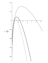
Figure 1: This figure shows the qualitative behavior of the metric component $g_{rr}^{-1}=1-\frac{b(r)}{r}$ with the shape function given by Eq. (51), for $\gamma=2$ and different values of the state parameter $\omega$. For the shown curves we have used $r_{0}=1$ and $\kappa=1$. The dashed and solid lines represent the behavior of $g_{rr}^{-1}$ with $\tilde{C}_{1}=\frac{1}{5}$ for $\omega=-2$ and $\omega=-\frac{1}{2}$ respectively. The dotted line represents the behavior of $g_{rr}^{-1}$ for $\omega=\frac{1}{3}$ and $\tilde{C}_{1}=-\frac{1}{5}$. The used parameter values satisfy the flare-out condition (55). The metric has the right signature $-+++$ for all $0<r_{0}<r<r_{b}$, allowing to exist wormhole configurations in this radial interval.

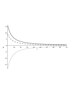
Figure 2: This figure shows the energy density $\rho(t_{0},r)$, where $t_{0}=const$, given by Eq. (52), for $\gamma=2$ and different values of the state parameter $\omega$. For the shown curves we have chosen $r_{0}=1$, $\kappa=1$ and $a_{0}=1$. The dashed and solid lines represent the behavior of the energy density for $\omega=-2$ and $\omega=-\frac{1}{2}$ respectively, choosing $\tilde{C}_{1}=\frac{1}{5}$. The dotted line represents the behavior of the energy density for $\omega=\frac{1}{3}$ and $\tilde{C}_{1}=-\frac{1}{5}$.

IV Discussion

In this paper we have obtained evolving $(N+1)$-dimensional wormhole solutions supported by polytropic matter. The considered wormhole models are described by a constant redshift function and generalizes the standard flat FRW spacetime. The matter source is defined by the “partially polytropic equation of state” (20), where the functions $\rho_{c}$ and $\rho_{w}$, depending on the time and radial coordinates respectively, have been introduced. This “partially polytropic equation of state” allows us to consider generalizations of the polytropic wormholes discussed in Ref. jamil . The generalization goes in two ways: first, we obtain a static $(N+1)$-dimensional extension of zero-tidal-force wormholes discussed by the authors of the mentioned Ref. jamil , and secondly a dynamic extension of the same static solution is obtained by introducing a scale factor with the help of the metric (2). The considered field equations lead to exponential expansion (contraction) of the scale factor due to the presence of the cosmological constant.

We discuss a particular $(3+1)$-dimensional expanding solution with the polytropic index $\gamma=2$. We show that it is possible to have wormhole geometries with positive energy density for any value $\omega<0$. For $\omega>0$ the energy density becomes always negative.

Finally, notice that from expression (III) we conclude that if $F\neq 0$, $N\geq 3$ and $0<\gamma\leq 1$, the solution is asymptotically flat FRW space-time at spatial infinity, since by requiring that $r\rightarrow\infty$ we obtain that $b(r)/r\approx r^{2-N}\rightarrow 0$. By taking into account Eq. (41) we conclude that the obtained asymptotic model corresponds to N+1-extension of the de-sitter cosmology for $\Lambda>0$. The Hubble rate is constant in any dimension. In standard 3+1-cosmology, the de-Sitter model is used to describe the early universe during cosmic inflation Burgess , and also the current accelerating expansion in the framework of the $\Lambda$CDM model LCDM . By neglecting ordinary matter, the dynamics of the universe is dominated by the cosmological constant, dubbed dark energy, and the expansion is exponential. The $\Lambda$CDM model has become the standard model for modern cosmology, since is the simplest model consistent with current observations.

In general, for $F\neq 0$, $N\geq 3$ and $0<\gamma\leq 1$, the obtained wormhole geometries far from the throat look like a flat FRW Universe. If the wormhole throat is located outside of the cosmological horizon of any observer, then he is not in causal contact with the throat. Thus, an observer located too far from the wormhole throat will see the Universe isotropic and homogeneous, and in principle he will be unable to make a decision about whether he lives in a space of constant curvature or in a space of a wormhole spacetime Cataldo15 .

V Acknowledgements

This work was partially supported by CONICYT through Grant FONDECYT N⁰ 1080530 and by the Dirección de Investigación de la Universidad del Bio-Bío through grants N⁰ DIUBB 121007 2/R and N⁰ GI121407/VBC (MC).

References

• (1) M. S. Morris, et al., Phys. Rev. Lett.  61, 1446 (1988);
• (2) M.S. Morris, K.S. Thorne, Am. J. Phys. 56, 395 (1988).
• (3) M. Visser, Lorentzian Wormholes: From Einstein to Hawking, (AIP, New York, 1995).
• (4) A. Anabalon and A. Cisterna, Phys. Rev. D 85, 084035 (2012).
• (5) G. A. S. Dias and J. P. S. Lemos, Phys. Rev.  D 82, 084023 (2010).
• (6) A. B. Balakin, J. P. S. Lemos and A. E. Zayats, Phys. Rev.  D 81, 084015 (2010).
• (7) M. Jamil, P. K. F. Kuhfittig, F. Rahaman and S. A. Rakib, Eur. Phys. J.  C 67, 513 (2010).
• (8) M. Jamil and M. U. Farooq, Int. J. Theor. Phys.  49, 835 (2010).
• (9) E. F. Eiroa, Phys. Rev.  D 80, 044033 (2009).
• (10) J. Estevez-Delgado and T. Zannias, Int. J. Mod. Phys. A 23, 3165 (2008).
• (11) M. Cataldo, P. Salgado and P. Minning, Phys. Rev.  D 66, 124008 (2002).
• (12) M. Cataldo, P. Meza and P. Minning, Phys. Rev.  D 83, 044050 (2011).
• (13) S. H. Hendi, J. Math. Phys.  52, 042502 (2011).
• (14) S. H. Hendi, Can. J. Phys.  89, 281 (2011).
• (15) I. Bochicchio and V. Faraoni, Phys. Rev.  D 82, 044040 (2010).
• (16) M. Jamil and M. Akbar, arXiv:0911.2556 [hep-th]; M. Jamil, Int. J. Theor. Phys.  50, 1602 (2011).
• (17) J. Hansen, D. i. Hwang and D. h. Yeom, JHEP 0911, 016 (2009).
• (18) A. DeBenedictis, R. Garattini and F. S. N. Lobo, Phys. Rev.  D 78, 104003 (2008).
• (19) P. F. Gonzalez-Diaz, Phys. Rev.  D 68, 084016 (2003).
• (20) O. Bertolami and R. Z. Ferreira, Phys. Rev. D 85, 104050 (2012).
• (21) F. Darabi, Can. J. Phys.  90, 461 (2012).
• (22) S. N. Sajadi and N. Riazi, Prog. Theor. Phys.  126, 753 (2011).
• (23) M. H. Dehghani and S. H. Hendi, Gen. Rel. Grav.  41, 1853 (2009).
• (24) M. Jamil et al., Eur. Phys. J. C 67, 513 (2010).
• (25) U. S. Nilsson, C. Uggla, Annals Phys.  286, 292 (2001).
• (26) S. Bayin, Phys. Rev. D 18, 2745 (1978).
• (27) P. M. Sa, Phys. Lett. B 467, 40 (1999).
• (28) M. Cataldo et al., Phys. Rev. D 79, 024005 (2009).
• (29) R. C. Myers, M. J. Perry, Ann. Phys.(NY) 172, 304 (1986).
• (30) C. P. Burgess, Class. Quant. Grav.  24, S795 (2007).
• (31) A. Kurek and M. Szydlowski, Astrophys. J.  675, 1 (2008); M. Douspis et al. [Archeops Collaboration], New Astron. Rev.  47, 755 (2003)
• (32) M. Cataldo and S. del Campo, Phys. Rev. D 85, 104010 (2012)