Theory of the Electron Spin Resonance in the Heavy Fermion Metal $\beta$-YbAlB${}_{4}\,$

Abstract

The heavy fermion metal $\beta$-YbAlB${}_{4}\,$exhibits a bulk room temperature conduction electron ESR signal which evolves into an Ising-anisotropic $f$-electron signal exhibiting hyperfine features at low temperatures. We develop a theory for this phenomenon based on the development of resonant scattering off a periodic array of Kondo centers. We show that the hyperfine structure arises from the scattering off the Yb atoms with nonzero nuclear spin, while the constancy of the ESR intensity is a consequence of the presence of crystal electric field excitations of the order of the hybridization strength.

Heavy fermion systems have been probed by a variety of experimental techniques and have provided great insights into the understanding of strong correlated systems. These systems are formed by a lattice of localized moments immersed in a conduction sea HF1 ; HF2 . An important class of heavy fermion metals exhibits the phenomenon of quantum criticality Si1 ; Si2 , and the recent discovery of an intrinsically quantum critical heavy fermion metal, $\beta$-YbAlB${}_{4}\,$Nak ; Mat ; Ram ; Far , with an unusual electron spin resonance (ESR) signal Hol has attracted great interest.

Traditionally, ESR is used as a probe of isolated magnetic ions in dilute rare-earth systems Bar . With the discovery of sharp bulk ESR absorption lines in certain heavy fermion materials, this experimental probe has emerged as a fascinating new tool to probe the low energy paramagnetic spin fluctuations in these materials. Normally, rare-earth ions display an ESR signal when they are weakly coupled to the surrounding conduction sea, acting as dilute “probe atoms”. A bulk $f$-electron ESR signal in heavy fermion metals is unexpected, for here, the lattice of local moments are strongly coupled to the conduction electron environment. Naively, one expects the ESR resonance to be washed out by the Kondo effect, yet surprisingly, sharp ESR lines have been seen to develop at low temperatures in a variety of heavy electron materials Kre ; Koc .

The case of $\beta$-YbAlB${}_{4}\,$, where the ESR signal evolves from a room temperature conduction electron signal into an Ising-anisotropic $f$-electron signal at low temperatures, is particularly striking. As the temperature is lowered, the $g$ factor changes from an isotropic $g\approx 2$ to an anisotropic $g$ factor characteristic of the magnetic Yb ions. Moreover, the signal develops hyperfine satellites characteristic of localized magnetic moments, yet the intensity of the signal remains constant, a signature of Pauli paramagnetism Hol . These results challenge our current understanding and motivate the development of a theory of spin resonance in the Anderson lattice.

Here, we formulate a phenomenological theory for the ESR of an Anderson lattice containing anisotropic magnetic moments. Our theory builds on earlier works AW ; Schl ; Han , focusing on the interplay between the lattice Kondo effect and the paramagnetic spin fluctuations while considering the effects of spin-orbit coupling, crystal electric field (CEF) and hyperfine coupling. We show that the key features of the observed ESR signal in $\beta$-YbAlB${}_{4}\,$, including the shift in the $g$ factor and the development of anisotropy, can be understood as a result of the development of a coherent many-body hybridization between the conduction electrons and the localized $f$ states. We are able to account for the emergence of hyperfine structure as a consequence of the static Weiss field created by the nuclei of the odd-spin isotopes of Yb. Moreover, using a spectral weight analysis, we show that the constancy of the intensity can be understood as a consequence of the intermediate value of the CEF excitations, comparable to the hybridization strength.

ESR measurements probe the low frequency transverse magnetization fluctuations in the presence of a static magnetic field. The power absorbed from a transverse ac electromagnetic field at fixed frequency $\nu_{0}$ as a function of the static external field $H$, is given by

$$P(\nu_{0},H)\propto\chi^{\prime\prime}_{+-}(\nu_{0},H),$$ (1)

where

$$\chi_{+-}(\nu,H)=-i\int_{0}^{\infty}dte^{i\nu t}\langle[M_{+}(t),M_{-}(0)]\rangle_{H}$$ (2)

is the dynamical transverse magnetic susceptibility and $M_{\pm}=M_{x}\pm iM_{y}$ are the raising and lowering components of the magnetization density.

In $\beta$-YbAlB${}_{4}\,$, the Yb ions are sandwiched between two heptagonal rings of boron atoms Nak , occupying a magnetic 4$f^{13}$ state with total angular momentum $J$=7/2. Crystal fields with sevenfold symmetry conserve $J_{z}$, splitting the $J$=7/2 Yb multiplet into four Kramers doublets, each with definite $|m_{J}|$. Based on the maximal degree of overlap, the Curie constant and the anisotropy of the magnetic susceptibility of $\beta$-YbAlB${}_{4}\,$, the low lying Yb doublet appears to be $|m_{J}=\pm 5/2\rangle$, with first excited state $|m_{J}=\pm 3/2\rangle$ And ; Lon .

We start with an infinite-$U$ Anderson lattice model, based on the overlap of the boron orbitals with the $|7/2,\alpha=\pm 5/2\rangle$ $f$-electron ground state doublet and the first excited CEF level, the pure $|7/2,\beta=\pm 3/2\rangle$ state, given by $H=H_{c}+H_{f}+H_{fc}-\mathbf{M}.\mathbf{H}$, where

$$H_{c} = \sum_{{\bf k},\sigma}\epsilon_{{\bf k}}c^{\dagger}_{{\bf k}\sigma}c_{{\bf k}\sigma},\qquad H_{f}=\sum_{j,\gamma}\epsilon_{f\gamma}f^{\dagger}_{\gamma}(j)f_{\gamma}(j),$$ (3)

$$H_{fc} = \sum_{j{\bf k}\sigma\gamma}(e^{-i{\bf k}{\bf R}_{j}}V_{{\bf k}\sigma\gamma}c^{\dagger}_{{\bf k}\sigma}X_{0\gamma}(j)+{\rm H.c.})$$ (4)

describe the conduction and $f$ bands, and the hybridization between them; $\mathbf{M}=\sum_{j}\mu_{B}\biggl{(}g_{c}\mathbf{S}_{c}(j)+g_{f}\mathbf{J}_{f}(j)\biggr{)}$ is the total magnetization, where $g_{c}=2$ and $g_{f}=8/7$ are the conduction and $f$-electron Landé $g$ factors and $\mathbf{J}_{f}$ is the total angular momentum operator of the $f$ states. The operator $c_{{\bf k}\sigma}^{\dagger}$ creates a conduction hole in the boron band with dispersion $\epsilon_{{\bf k}}$. The composite $X_{0\gamma}=(b^{\dagger}f_{\gamma})\equiv|4f^{14}\rangle\langle 4f^{13},\gamma|$ is the Hubbard operator between the $|4f^{13},\gamma\rangle\equiv f^{\dagger}_{\gamma}|0\rangle$, “hole” states of the Yb³⁺ ion and the filled shell Yb²⁺ state $|4f^{14}\rangle\equiv b^{\dagger}|0\rangle$, written using a slave boson representation. The azimuthal quantum number $\gamma\equiv m_{J}$ has values $\gamma\in[\pm 5/2,\pm 3/2]$ corresponding to the ground state doublet with energy $\epsilon_{f\pm 5/2}=\epsilon_{f}$ and the next CEF level, with energy $\epsilon_{f\pm 3/2}=\epsilon_{f}+{\Delta_{X}}$.

We employ a mean-field approximation $X_{0\gamma}(j)\rightarrow rf_{\gamma(j)}$, where the mean-field amplitude of the slave boson, $r=|\langle b_{j}\rangle|$ describes the emergence of the Abrikosov-Suhl resonance at each site, resulting from Kondo screening. In the mean field theory, $H\rightarrow H_{c}+\tilde{H}_{f}+\tilde{H}_{fc}$, where

$$\tilde{H}_{f} = \sum_{{\bf k}\gamma}\tilde{\epsilon}_{f\gamma}f_{{\bf k}\gamma}^{\dagger}f_{{\bf k}\gamma}+\lambda(r^{2}-1),$$ (5)

$$\tilde{H}_{fc} = \sum_{{\bf k}\sigma\gamma}\bigl{[}c^{\dagger}_{{\bf k}\sigma}\tilde{V}_{{\bf k}\sigma\gamma}f_{{\bf k}\gamma}+{\rm h.c.}\bigr{]},$$ (6)

with $\tilde{V}_{{\bf k}\sigma\gamma}=V_{{\bf k}\sigma\gamma}r$ and $\tilde{\epsilon}_{f\gamma}=\epsilon_{f\gamma}+\lambda$ the renormalized quasiparticle hybridization and $f$-level energy, and $\lambda$ the Lagrange multiplier that enforces the average constraint $\langle n_{f}\rangle+\langle b^{\dagger}b\rangle=1$. The temperature dependence of the many body amplitude $r(T)$ and $\lambda(T)$ determines the evolution of the ESR signal.

In the ground state, the ratio $\tilde{V}^{2}/W\sim T_{K}$ determines the Kondo temperature $T_{K}$, where $\tilde{V}$ is the characteristic size of the hybridization and $W$ is the conduction electron bandwidth. The degree of magnetic anisotropy in the Kondo lattice is set by the size of the crystal field splitting ${\Delta_{X}}$. In a Kondo impurity, one can project out the crystal field excited states, provided ${\Delta_{X}}/T_{K}{{\lower 4.0pt\hbox{$>$}}\atop\widetilde{\ \ \ }}1$, and crystal symmetry prevents any admixture of the projected states with the Abrikosov-Suhl resonance. However, in a Kondo lattice the nonconservation of crystal symmetry becomes important once $\Delta_{X}{{\lower 4.0pt\hbox{$>$}}\atop\widetilde{\ \ \ }}\tilde{V}\sim\sqrt{T_{K}W}$, a situation that can occur even though $\Delta_{X}\gg T_{K}$. In this situation, the hybridization will admix the mobile $f$ quasiparticles with the higher crystal field states. We shall show that this produces significant modification to the magnetization operator of the quasiparticles. Thus, there are three regimes of interest:

1. Ising limit: $\Delta_{X}/\tilde{V}\gg 1$, ${\Delta_{X}}/T_{K}\gg 1$,

2. Intermediate anisotropy: $\Delta_{X}/\tilde{V}{{\lower 4.0pt\hbox{$>$}}\atop\widetilde{\ \ \ }}1$, ${\Delta_{X}}/T_{K}\gg 1$,

3. Weak anisotropy: $\Delta_{X}/\tilde{V}<1$.

Although $\beta$-YbAlB${}_{4}\,$almost certainly lies in the second category, the Ising limit captures most of the physics. In this limit, the $\pm 3/2$ states are projected out, leading to a two-band model in which the matrix elements of the transverse $f$ magnetization $J_{f}^{\pm}$ are absent. The ESR signal, then, is determined by the spin dynamics of the conduction electrons in the presence of the lattice Kondo effect, given by $P(\nu,H)\propto\chi^{\prime\prime}_{c+-}(\nu,H)$. As a first step we examine this limit, using a simplified model in which the hybridization is spin diagonal and its complex momentum dependence is ignored, replacing $\tilde{V}_{{\bf k}\sigma\gamma}\rightarrow\tilde{V}\underline{1}$. In mean-field theory,

$$\chi_{c+-}(i\nu_{n})=-\mu_{B}^{2}T\sum_{m}G_{c\downarrow}({\bf k},i\tilde{\omega}_{m}+i\nu_{n})G_{c\uparrow}({\bf k},i\tilde{\omega}_{m})$$ (7)

where $G_{c\sigma}(z)=\left[z-\epsilon_{{\bf k}\sigma}-\Sigma_{c\sigma}(z)\right]^{-1}$ is the conduction electron propagator and $\Sigma_{c\sigma}(z)={V}^{2}r^{2}/(z-\tilde{\epsilon}_{f\sigma})$ is the self-energy generated by resonant scattering off $f$ states. Here vertex corrections have been neglected and the spin relaxation has been included as a white noise Weiss field acting on conduction and $f$ electrons, shifting the Matsubara frequency by the spin-relaxation rate, $\tilde{\omega}_{m}=\omega_{m}+i\frac{\Gamma}{2}{\rm sgn}(\omega_{m})$. Carrying out the momentum sum as an energy integral, and expanding the self-energy to linear order in frequency, at low temperatures we obtain

$$\chi_{c+-}(\nu-i\delta,H)=\mu_{B}^{2}Z_{c}N_{c}(0)\left(\frac{g^{*}\mu_{B}H+i\Gamma}{g^{*}{\mu}_{B}H+i\Gamma-\nu}\right).$$ (8)

Here, $N_{c}(0)$ is the density of states of the conduction electrons, $Z_{c}=(1-\partial\Sigma_{c}/\partial\omega)^{-1}=(1+V^{2}r^{2}/\tilde{\epsilon}_{f}^{2})^{-1}$ is the conduction electron quasiparticle weight and

$$g^{*}=g_{c}Z_{c}+g_{f}^{*}(1-Z_{c})$$ (9)

is the effective $g$ factor of the heavy quasiparticles at the Fermi surface (FS), where $g_{f}^{*}=g_{f}(2m_{J})=5.7$. At high temperatures, $g^{*}\approx 2$ reflects the conduction character of the FS, but as the temperature is lowered the $g$ factor rises towards $g_{f}^{*}$ as the FS acquires $f$ character. The evolution of $g^{*}(T)$, computed using the temperature-dependent mean-field parameters (Fig. 1), is qualitatively similar to that observed in $\beta$-YbAlB${}_{4}\,$, but the asymptotic value at low temperatures is twice as large as that seen experimentally. Details of the computation can be seen in the Supplemental Material. In the Ising limit, the $f$ band responds uniquely to $z$-axis fields, so that when a field is applied at an angle $\theta$ from the plane perpendicular to the $z$ axis, we may decompose the $g$ factor in components parallel and perpendicular to the $c$ axis:

$$g^{*}(\theta) = \sqrt{(g^{*}_{\parallel}\sin\theta)^{2}+(g^{*}_{\perp}\cos\theta)^{2}}.$$ (10)

At high temperatures, $g^{*}(\theta)=g_{c}$ is isotropic, but at low temperatures, $g^{*}(\theta)\sim 5g_{f}\sin\theta$ exhibits Ising anisotropy (Fig. 1 inset).

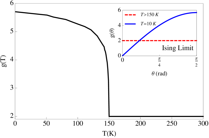
Figure 1: Temperature dependence of the thermally averaged $g$ factor. The parameters used were $\epsilon_{f}=-0.15eV$ and $V=0.26eV$. See details of the mean field solution in the Supplemental Material. The inset shows the anisotropy of the $g$ factor in the Ising limit.

Next, we consider the effect of hyperfine coupling on the Kondo lattice ESR signal. A small isotopic percentage ($n_{i}\approx$14%) of the Yb atoms in $\beta$-YbAlB${}_{4}\,$carry nuclear spins, which give rise to a hyperfine coupling between the $f$ states and the nuclei Hol . The $f$ electrons at these sites experience a Weiss field of magnitude $A$ that shifts the central energy $\tilde{\epsilon}_{f}$ of the Abrikosov-Suhl resonance. When we impurity average over the positions of the isotopic impurities, this modifies the conduction electron self-energy $\Sigma_{c\gamma}(z)\rightarrow\Sigma_{c\gamma}(z)+\delta\Sigma_{c\gamma}(z)$, where

$$\delta\Sigma_{c\gamma}(z) =$$ (11)

$$= \frac{n_{i}\tilde{V}^{2}}{2}\sum_{\sigma=\pm 1}\left(\frac{1}{z-\tilde{\epsilon}_{f\gamma}+A\sigma}-\frac{1}{z-\tilde{\epsilon}_{f\gamma}}\right)$$ (12)

with the crosses representing the hyperfine field $A\sigma$ ($\sigma=\pm 1$). The resulting electron self energy

$$\Sigma_{c\gamma}(z)=\frac{(1-n_{i})\tilde{V}^{2}}{z-\tilde{\epsilon}_{f\gamma}}+\frac{\frac{n_{i}}{2}\tilde{V}^{2}}{z-\tilde{\epsilon}_{f\gamma}+A}+\frac{\frac{n_{i}}{2}\tilde{V}^{2}}{z-\tilde{\epsilon}_{f\gamma}-A}$$ (13)

contains two extra resonances, shifted by the hyperfine coupling constant $A$, which lead to two corresponding side peaks in the ESR lines at low temperatures, as shown in Fig. 2. Thus, we are able to interpret the appearance of hyperfine peaks in the ESR signal of $\beta$-YbAlB${}_{4}\,$as a consequence of the hyperfine splitting of the resonant scattering in this Kondo lattice.

Figure 2: ESR signal computed using the mean-field theory, including the effect of hyperfine coupling in the Abrikosov-Suhl resonance. Here $A=7.5\times 10^{-6}eV$ and $\Gamma=7.2\times 10^{-7}eV$. The low temperature curve was rescaled by a factor of 10. Note the development of satellite peaks at low temperatures.

Now we turn to a discussion of the ESR signal intensity in $\beta$-YbAlB${}_{4}\,$. Here, we employ a sum rule relating the quasiparticle, or Pauli component of the magnetization to the ESR intensity. The ESR intensity is the field integral of the absorbed power, $I_{ESR}\propto\int_{0}^{H_{max}}\chi_{+-}^{\prime\prime}(\nu_{0},H)dH$, where $H_{max}$ is the maximum field applied and $\nu_{0}$ is the fixed ESR frequency. We can write this in the form

$$I_{ESR}\propto H_{0}\int_{0}^{H_{max}}\frac{\chi_{+-}^{\prime\prime}(\nu_{0},H)}{\nu_{0}}g^{*}\mu_{B}dH,$$ (14)

where $H_{0}=\nu_{0}/(2g^{*}\mu_{B})$ is the resonance field. Now since the integrand is an even function of $\nu_{0}-2g^{*}\mu_{B}H$, it follows that $\chi_{+-}^{\prime\prime}(\nu_{0},H)=\chi^{\prime\prime}_{+-}(\nu,H_{0})$, where $\nu=2g^{*}\mu_{B}H$. Writing $d\nu=2g^{*}\mu_{B}dH$, then

$$I_{ESR}\propto\frac{H_{0}}{2}\int_{0}^{\nu_{max}}\frac{\chi_{+-}^{\prime\prime}(\nu,H_{0})}{\nu}d\nu,$$ (15)

where $\nu_{max}=2g^{*}\mu_{B}H_{max}$ and we have used the narrowness of the peak to replace $\nu_{0}\rightarrow\nu$ in the denominator. There is also a sum rule for the total transverse static susceptibility, given by the Kramers-Krönig relation:

$$\chi_{+-}^{\prime}(0,H_{0})=\frac{1}{2\pi}\int_{-\infty}^{\infty}\frac{\chi^{\prime\prime}_{+-}(\nu,H_{0})}{\nu}d\nu.$$ (16)

In anisotropic $f$-electron systems like $\beta$-YbAlB${}_{4}\,$, the transverse susceptibility is dominated by Van Vleck paramagnetism, and is temperature independent. In this situation, (16) plays the role of a magnetic $f$-sum rule. In fact, the static susceptibility $\chi^{\prime}(\nu=0,H_{0})=\chi_{\rm Pauli}+\chi_{VV}$ is a sum of Pauli and Van Vleck (VV) susceptibilities, where the Pauli contribution derives from low-frequency spin-flip processes, lying within the frequency range detected by ESR, whereas the Van Vleck contributions derive from much larger crystal-field frequencies. In this way, we see that the ESR intensity measures the Pauli component of the transverse magnetization,

$$I_{ESR}(T)\propto 2\pi H_{0}\chi_{\rm Pauli}(T).$$ (17)

Experimentally, both the transverse static susceptibility ($\chi_{Total}(T)=\chi_{0}$, Mac ) and the ESR intensity ($I_{ESR}(T)=I_{0}$, Hol ) are temperature independent. While the large constant value of the total susceptibility reflects its Van Vleck character, telling us that the total spectral weight in Eq. (16) is conserved, the temperature independence of the ESR intensity means that the Pauli contribution to the spectral weight is also conserved. In the Ising limit, as the hybridization turns on, there is a large reduction in the conduction electron character of the FS, giving rise to a much reduced transverse magnetization and ESR intensity. Thus to account for these features we need to reinstate the finite CEF.

In the presence of a CEF level, the decomposition of the quasiparticles into conduction and $f$ electrons contains an additional amplitude to be in the excited crystal field state $|f_{3/2}\beta\rangle$,

$$|n{\bf k}\sigma\rangle=a_{n\sigma}|c{\bf k}\sigma\rangle+b_{n\alpha}|f_{5/2}\alpha\rangle+c_{n\beta}|f_{3/2}\beta\rangle.$$ (18)

The low temperature Pauli part of the transverse susceptibility is written as $\chi_{Pauli}=N^{*}(0)|\langle 1{\bf k}\uparrow|M_{+}|1{\bf k}\downarrow\rangle|^{2}$, where $N^{*}(0)\sim 1/T_{K}$ is the low temperature quasiparticle density of states; thus, the ratio between the zero and room temperature intensities is given by

$$\frac{I_{ESR}(0)}{I_{ESR}(T>T_{K})}\propto\frac{N^{*}(0)}{N_{c}(0)}\frac{|\langle 1{\bf k}\uparrow|M_{+}|1{\bf k}\downarrow\rangle|^{2}}{\mu_{B}^{2}},$$ (19)

where $N_{c}(0)\sim 1/W$ is the conduction electron density of states and the matrix element at high temperatures is equal to $\mu_{B}^{2}$. The matrix element of the lower band ($n$=1) is $|\langle 1{\bf k}\uparrow|M_{+}|1{\bf k}\downarrow\rangle|^{2}=\mu_{B}^{2}|a_{1\uparrow}a_{1\downarrow}+g_{f}\sqrt{3}(b_{1\uparrow}c_{1\downarrow}+c_{1\uparrow}b_{1\downarrow})|^{2}$. Transitions between the $5/2$ and $3/2$ states happens via an intermediate conduction state:

giving rise to a transition matrix element between the crystal field states of magnitude $\tilde{V}^{2}/W\sim T_{K}$. The ground-state quasiparticle amplitudes are, thus, of order $(\sqrt{T_{K}/W},1,{T_{K}/{\Delta_{X}}})$, respectively. In the pure Ising limit ($\Delta_{X}\rightarrow\infty$) we have $I_{ESR}(0)/I_{ESR}(T>T_{K})\sim T_{K}/W\ll 1$ but at intermediate anisotropy ($\Delta_{X}/\tilde{V}{{\lower 4.0pt\hbox{$>$}}\atop\widetilde{\ \ \ }}1$) new contributions to the transverse magnetization appear and it acquires a value of order unity, $I_{ESR}(0)/I_{ESR}(T>T_{K})\sim{WT_{K}}/{\Delta_{X}^{2}}=(\tilde{V}/\Delta_{X})^{2}\sim 1$.

The preservation of ESR intensity at low temperatures can also be understood in terms of magnetic sum rules (Fig. 3). From Eq.( 15), we see that the ESR signal is a kind of “magnetic Drude peak” in the dynamical spin susceptibility, slightly shifted from zero frequency by the applied magnetic field. In a simple hybridization model with Ising spins, there is a transfer of magnetic Drude weight to high energies, a magnetic analog of the spectral weight transfer which develops in the optical conductivity Aep . However, when a crystal field is introduced, the transfer of spectral weight to high energies is compensated by the downward transfer of spectral weight from the crystal field levels due to admixture of $\pm 3/2$ states into the heavy bands. This preserves a fraction of order $O(\tilde{V}/{\Delta_{X}})^{2}$ of the low frequency spectral weight.

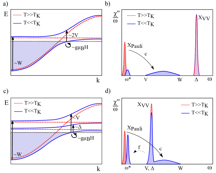
Figure 3: Schematic plots of the bands a) Ising limit and c) Intermediate anisotropy. The arrows indicate the order of magnitude of the possible excitations. Imaginary part of the transverse spin susceptibility b) Ising limit and d) Intermediate anisotropy The arrows indicate the flow of spectral weight as the temperature is lowered.

Although we have not calculated it in detail, we note that the intermediate anisotropy limit allows us to understand the reduction of the ESR anisotropy. In particular, the momentum-space anisotropy of the hybridization matrices $V_{{\bf k}\sigma\gamma}$ will introduce a $k$-dependent rotation of the field quantization axes. Quite generally, this effect will broaden the ESR line, reducing both the average value of the $g$ factor and the degree of anisotropy of the signal.

Our theory suggests various experiments to shed further light on our understanding of the spin paramagnetism of heavy fermion systems. In particular, since $\beta$-YbAlB${}_{4}\,$is a Pauli limited superconductor, we expect its upper critical field $H_{c2}$ to be inversely proportional to the effective $g$ factor, so measuring the angular dependence of $H_{c2}$ would allow us to independently confirm the size and anisotropy of the $g$ factor. It would also be interesting to examine whether similar Ising anisotropic systems, such as CeAl₃ or URu₂Si₂ and the quasicrystal YbAlAu Deg exhibit ESR signals. Our emergent hybridization model also raises many interesting questions. For example, what is the underlying origin of the sharp $f$-electron ESR line, which we have modeled phenomenologically? Moreover, is there a connection between the ESR resonance and quantum criticality in both $\beta$-YbAlB${}_{4}\,$Hol ; Nak ; Mat ; Ram ; Far and YbRh₂Si${}_{2}\,$Sic1 ; Cus ? Tantalizingly, $\alpha$-YbAlB₄, a system with a structure locally similar to the $\beta$ phase does not exhibit a $g$ shift, yet iron doping appears to drive it into quantum criticality where a $g$ shift develops in the ESR Pas , suggesting these two effects are closely related. Clearly, these are issues for further investigation.

The authors would like to thank E. Abrahams, P. G. Pagliuso, C. Rettori, R. R. Urbano, F. Garcia and L. M. Holanda for discussions related to the ESR phenomena. This research was supported by National Science Foundation Grants No. DMR-0907179 and No. DMR-1309929.

I Supplemental Material

As mentioned in the main text, we employ a mean-field approximation $X_{0\gamma}(j)\rightarrow rf_{\gamma}(j)$, where the mean-field amplitude of the slave boson, $r=|\langle b_{j}\rangle|$ describes the emergence of the Abrikosov-Suhl resonance at each site, resulting from Kondo screening. In the mean field theory, $H\rightarrow H_{c}+\tilde{H}_{f}+\tilde{H}_{fc}$, where

$$H_{c} = \sum_{{\bf k},\sigma}\epsilon_{{\bf k}}c^{\dagger}_{{\bf k}\sigma}c_{{\bf k}\sigma},$$ (20)

$$\tilde{H}_{f} = \sum_{{\bf k}\gamma}\tilde{\epsilon}_{f\gamma}f_{{\bf k}\gamma}^{\dagger}f_{{\bf k}\gamma}+\lambda(r^{2}-1),$$ (21)

$$\tilde{H}_{fc} = \sum_{{\bf k}\sigma\gamma}\bigl{[}c^{\dagger}_{{\bf k}\sigma}\tilde{V}_{{\bf k}\sigma\gamma}f_{{\bf k}\gamma}+{\rm h.c.}\bigr{]},$$ (22)

where $\tilde{V}_{{\bf k}\sigma\gamma}=V_{{\bf k}\sigma\gamma}r$ and $\tilde{\epsilon}_{f\gamma}=\epsilon_{f\gamma}+\lambda$ are the renormalized quasiparticle hybridization and f-level energy, respectively. The Lagrange multiplier $\lambda$ enforces the average constraint $\langle n_{f}\rangle+\langle b^{\dagger}b\rangle=1$.

Diagonalizing the mean field Hamiltonian within the assumption that the hybridization is momentum independent and spin-diagonal, one finds the energy bands:

$$E_{{\bf k}\sigma}^{\pm}=\frac{\epsilon_{{\bf k}\sigma}+\tilde{\epsilon}_{f\gamma}}{2}\pm\sqrt{\left(\frac{\epsilon_{{\bf k}\sigma}-\tilde{\epsilon}_{f\gamma}}{2}\right)^{2}+\tilde{V}^{2}}.$$ (23)

The temperature dependence of the ESR signal is determined by the temperature evolution of $r(T)$ and $\lambda(T)$. These are computed by the extremization the free energy, that can be written as:

$$F=-\beta^{-1}\sum_{{\bf k},\sigma,n}ln(1+e^{-\beta E_{{\bf k}\sigma}^{n}})+\lambda(r^{2}-1),$$ (24)

where $n=\pm$ is the band index and $\beta^{-1}=k_{B}T$.

The extremization of the free energy with respect to the mean field parameters $r$ and $\lambda$ are determined by:

$$\frac{\partial F}{\partial r}=0,\hskip 28.45274pt\frac{\partial F}{\partial\lambda}=0,$$ (25)

what gives two coupled equations:

$$\sum_{{\bf k},\sigma,n}f(E_{{\bf k}\sigma}^{n})\frac{\partial E_{{\bf k}\sigma}^{n}}{\partial r}+2\lambda r=0,$$ (26)

$$\sum_{{\bf k},\sigma,n}f(E_{{\bf k}\sigma}^{n})\frac{\partial E_{{\bf k}\sigma}^{n}}{\partial\lambda}+r^{2}-1=0$$ (27)

that are solved numerically.

For the numerical solution we use the equations above in a two dimensional square lattice with hopping parameter $t=1eV$, chemical potential $\mu=-0.2eV$. The location of the f-level is $\epsilon_{f}=-0.15eV$ and $V=0.26eV$. The temperature evolution of the mean field parameters is shown in the figure below:

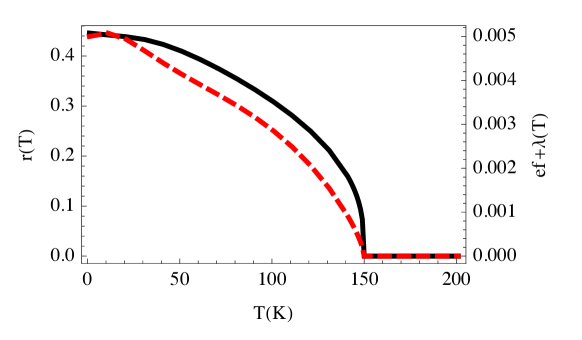
Figure 4: Temperature dependence of the mean field parameters r (solid line) and $\lambda$ (dashed line) solved numerically.

In the main text we define $g^{*}=g_{c}Z_{c}+g_{f}^{*}(1-Z_{c})$ as a simple closed form for the effective g-factor. This was a zero temperature calculation and gives only the value of the g-factor at the FS, what is a rough estimate of the real value of this parameter.

We calculated the temperature dependence of the g-factor from the ratio between the photon energy $\nu_{0}$ and the Zeeman energy $2\mu_{B}H_{res}(T)$ at the resonance field, $g(T)=\nu_{0}/2\mu_{B}H_{res}(T)$. $H_{res}$ was determined from the maximum of the imaginary part of the dynamical spin susceptibility

$$\chi_{c+-}(\nu_{0}-i\delta,H)=-\mu_{B}^{2}\sum_{{\bf k},n,m=\pm}Z_{{\bf k}\downarrow}^{n}Z_{{\bf k}\uparrow}^{m}\frac{f(E_{{\bf k}\downarrow}^{n})-f(E_{{\bf k}\uparrow}^{m})}{-\nu_{0}+E_{{\bf k}\downarrow}^{n}-E_{{\bf k}\uparrow}^{m}+i\Gamma},$$ (28)

where,

$$Z_{{\bf k}\sigma}^{n}=\frac{E_{{\bf k}\sigma}^{n}-\epsilon_{f\sigma}}{E_{{\bf k}\sigma}^{n}-E_{{\bf k}\sigma}^{-n}},$$ (29)

calculated at fixed frequency, as a function of field. In our actual calculations we used the experimental value for the fixed ESR frequency $\nu_{0}=3.9\times 10^{-5}$eV (for the X-band frequency of $9.5$ GHz) and $\Gamma=7.2\times 10^{-7}eV$. The numerical solution is plotted in Fig.1 in the main text.

References

- (1) A. C. Hewson, The Kondo problem to heavy fermions, Cambridge University Press (1993).
- (2) P. Coleman in Handbook of Magnetism and Advanced Magnetic Materials, Vol. 1, John Wiley and Sons (2007).
- (3) P. Gegenwart, Q. Si and F. Steglich, Nature Physics 4, 186 (2008).
- (4) Q. Si and F. Steglich, Science 329, 1161 (2010).
- (5) S. Nakatsuji, K. Kuga, Y. Machida, T. Tayama, T. Sakakibara, Y. Karaki, H. Ishimoto, S. Yonezawa, Y. Maeno, E. Pearson, G. G. Lonzarich, L. Balicas, H. Lee and Z. Fisk, Nat. Phys. 4, 603 (2008).
- (6) Y. Matsumoto, S. Nakatsuji, K. Kuga, Y. Karaki, N. Horie, Y. Shimura, T. Sakakibara, A. H. Nevidomskyy and P. Coleman, Science 21, 316 (2011).
- (7) A. Ramires, P. Coleman, A. H. Nevidomskyy and A. M. Tsvelik, Phys. Rev. Lett. 109, 176404 (2012).
- (8) E. C. T. O’Farrell, Y. Matsumoto, and S. Nakatsuji, Phys. Rev. Lett. 109, 176405 (2012).
- (9) L. M. Holanda, J. M. Vargas, W. Iwamoto, C. Rettori, S. Nakatsuji, K. Kuga, Z. Fisk, S. B. Oseroff and P. G. Pagliuso, Phys. Rev. Lett. 107, 026402 (2011).
- (10) S. E. Barnes, Adv. in Phys. 30, 801 (1980).
- (11) C. Krellner, T. Förster, H. Jeevan, C. Geibel and J. Sichelschmidt , Phys. Rev. Lett. 100, 066401 (2008).
- (12) B. I. Kochelaev, S. I. Belov, A. M. Skvortsova, A. S. Kutuzov, J. Sichelschmidt, J. Wykhoff, C. Geibel, F. Steglich, Eur. Phys. J. B 72, 485 (2009).
- (13) E. Abrahams and P. Wölfle, Phys. Rev. B 78, 104423 (2008).
- (14) P. Schlottmann, Phys. Rev. B 79, 045104 (2009).
- (15) K. Hanzawa, K. Yosida, K. Yamada, Prog. Theor. Phys. 81, 960 (1989).
- (16) A. H. Nevidomskyy and P. Coleman, Phys. Rev. Lett. 102, 077202 (2009).
- (17) D. A. Tompsett, Z. P.Yin, G. G. Lonzarich, W. E. Pickett, Phys. Rev. B 82, 235101 (2010).
- (18) R. T. Macaluso, S.Nakatsuji, K. Kuga, E. L. Thomas, Y. Machida, Y. Maeno, Z. Fisk and J. Y. Chan, Chem. Mater. 19, 1918 (2007).
- (19) Z. Schlesinger, Z. Fisk, Hai-Tao Zhang, M. B. Maple, J. F. DiTusa and G. Aeppli, Phys. Rev. Lett. 71, 1748 (1993).
- (20) K. Deguchi, S. Matsukawa, N. K. Sato, T. Hattori, K. Ishida, H.Takakura andT. Ishimasa, Nat. Mater. 11, 1013 (2012).
- (21) J. Sichelschmidt, V. A. Ivanshin, J. Ferstl, C. Geibel and F. Steglich, Phys. Rev. Lett. 91, 156401 (2003).
- (22) J. Custers, P. Gegenwart, H. Wilhelm, K. Neumaier, Y. Tokiwa, O. Trovarelli, C. Geibel, F. Steglich, C. Pépin and P. Coleman, Nature 424, 524 (2003).
- (23) P. G. Pagliuso, C. Rettori and L. M. Holanda (private communication).