Network Formation Games with Heterogeneous Players and the Internet Structure

Abstract

We study the structure and evolution of the Internet’s Autonomous System (AS) interconnection topology as a game with heterogeneous players. In this network formation game, the utility of a player depends on the network structure, e.g., the distances between nodes and the cost of links. We analyze static properties of the game, such as the prices of anarchy and stability and provide explicit results concerning the generated topologies. Furthermore, we discuss dynamic aspects, demonstrating linear convergence rate and showing that only a restricted subset of equilibria is feasible under realistic dynamics. We also consider the case where utility (or monetary) transfers are allowed between the players.

Eli .A. Meirom, Shie Mannor, Ariel Orda, 2014. Network Formation Games and the Internet Structure. This research was supported in part by the European Union through the CONGAS project (http://www.congas-project.eu/) in the 7th Framework Programme.

1 Introduction

The structure of large-scale communication networks, in particular that of the Internet, has carried much interest. The Internet is a living example of a large, self organized, many-body complex system. Understanding the processes that shape its topology would provide tools for engineering its future.

The Internet is composed of multiple Autonomous Systems (ASs), which are contracted by different economic agreements. These agreements dictate the routing pathways among the ASs. With some simplifications, we can represent the resulting network as a graph, where two nodes (ASs) are connected by a link if traffic is allowed to traverse through them. The statistical properties of this complex graph, such as the degree distribution, clustering properties etc., have been extensively investigated [15, 27, 25]. However, such findings per se lack the ability to either predict the future evolution of the Internet nor to provide tools for shaping its development.

Most models, notably “preferential attachment” [2], emulate the network evolution by probabilistic rules and recover some of the statistical aspects of the network. However, they fail to account for many other features of the network [11], as they treat the ASs as passive elements rather than economic, profit-maximizing entities. Indeed, in this work we examine some findings that seem to contradict the predictions of such models but are explained by our model.

Game theory is by now a widely used doctrine in network theory and computer science in general. It describes the behavior of interacting rational agents and the resulting equilibria, and it is one of the main tools of the trade in estimating the performance of distributed algorithms [9]. In the context of communication networks, game theory has been applied extensively to fundamental control tasks such as bandwidth allocation [18], routing [2, 23] and flow control [1]. It was also proven fruitful in other networking domains, such as network security [24] and wireless network design [10].

Recently, there has been a surge of studies exploring networks created by rational players, where the costs and utility of each player depend on the network structure. Some studies emphasized the context of wireless networks [21] whereas other discussed the inter-AS topology [5, 3]. These works fall within the realm of network formation games [17, 16]. The focus of those studies has been to detail some specific models, and then investigate the equilibria’s properties, e.g., establishing their existence and obtaining bounds on the “price of anarchy” and ”price of stability”. The latter bound (from above and below, correspondingly) the social cost deterioration at an equilibrium compared with a (socially) optimal solution. Taking a different approach,Lodhi et al. [19] present an analytically-intractable model , hence simulations are used in order to obtain statistical characteristics of the resulting topology.

Nonetheless, most of these studies assume that the players are identical, whereas the Internet is composed of many types of ASs, such as minor ISPs, CDNs, tier-1 ASs etc. Only a few studies have considered the effects of heterogeneity on the network structure. Addressing social networks, [26] describes a network formation game in which the link costs are heterogeneous and the benefit depends only on a player’s nearest neighbors (i.e., no spillovers). In [17], the authors discuss directed networks formation, where the information (or utility) flows in one direction along a link; the equilibria’s existence properties of the model’s extension to heterogeneous players was discussed in [3].

With very few exceptions, e.g., [6], the vast majority of studies on the application of game theory to networks, and network formation games in particular, focus on static properties. However, it is not clear that the Internet, nor the economic relations between ASs, have reached an equilibrium. In fact, dynamic inspection of the inter-AS network presents evidence that the system may in fact be far from equilibrium. Indeed, new ASs emergence, other quit business or merge with other ASs, and new contracts are signed, often employing new business terms. Hence, a dynamic study of inter-AS network formation games is called for.

The aim of this study is to address the above two major challenges, namely heterogeneity and dynamicity. Specifically, we establish an analytically-tractable model, which explicitly accounts for the heterogeneity of players. Then, we investigate both its static properties as well as its dynamic evolution.

We model the inter-AS connectivity as a network formation game with heterogeneous players that may share costs by monetary transfers. We account for the inherent bilateral nature of the agreements between players, by noting that the establishment of a link requires the agreement of both nodes at its ends, while removing a link can be done unilaterally. The main contributions of our study are as follows:

• We evaluate static properties of the considered game, such as the prices of anarchy and stability and characterize additional properties of the equilibrium topologies. In particular, the optimal stable topology and examples of worst stable topologies are expressed explicitly.

• We discuss the dynamic evolution of the inter-AS network, calculate convergence rates and basins of attractions for the different final states. Our findings provide useful insight towards incentive design schemes for achieving optimal configurations. Our model predicts the existence of a settlement-free clique, and that most of the other contracts between players include monetary transfers.

Game theoretic analysis is dominantly employed as a “toy model” for contemplating about real-world phenomena. It is rarely confronted with real-world data, and to the best of our knowledge, it was never done in the context of inter-AS network formation games. In this study we go a step further from traditional formal analysis, and we do consider real inter-AS topology data. A preliminary data analysis, which supports our findings, appears in the appendix.

The paper is organized as follows. In the next section, we describe our model. We discuss two variants, corresponding to whether utility transfers (e.g., monetary transfers) are allowed or not. We present static results in Section 3, followed by dynamic analysis in Section 4. Section 5 addresses the case of permissible monetary transfers, both in the static and dynamic aspects. Finally, conclusions are presented in Section 6. Full proofs and some technical details are omitted from this version and can be found in the appendix.

2 Model

Our model is inspired by the inter-AS interconnection network, which is formed by drawing a link between every two ASs that mutually agree to allow bidirectional communication. The utility of each AS, or player, depends on the resulting graph’s connectivity. We can imagine this as a game in which a player’s strategy is defined by the links it would like to form, and, if permissible, the price it will be willing to pay for each. In order to introduce heterogeneity, we consider two types of players, namely major league (or type-A) players, and minor league (or type-B) players. The former may represent main network hubs (e.g., in the context of the Internet, Level-3 providers), while the latter may represent local ISPs.

The set of type-A (type B) players is denoted by $T_{A}$ ( $T_{B}$). A link connecting node $i$ to node $j$ is denoted as either $(i,j)$ or $ij$. The total number of players is $N=|T_{A}|+|T_{B}|$, and we always assume $N\geq 3$. The shortest distance between nodes $i$ and $j$ is the minimal number of hops along a path connecting them and is denoted by $d(i,j)$. Finally, The degree of node $i$ is denoted by $deg(i)$.

2.1 Basic model

The utility of every player depends on the aggregate distance from all other players. Most of the previous studies assume that each player has a specific traffic requirement for every other player. This results in a huge parameter space. However, it is reasonable to assume that an AS does not have exact flow perquisites to every individual AS in the network, but would rather group similar ASs together according to their importance. Hence, a player would have a strong incentive to maintain a good, fast connection to the major information and content hubs, but would relax its requirements for minor ASs. Accordingly, we represent the connection quality between players as their graph distance, since many properties depend on this distance, for example delays and bandwidth usage. As the connection to major players is much more important, we add a weight factor $A$ to the cost function in the corresponding distance term. The last contribution to the cost is the link price, $c.$ This term represents factors such as the link’s maintenance costs, bandwidth allocation costs etc.

The structure of our cost function extends the work of Fabrikant et al. [14] and Corbo and Parkes [12]. This model was studied extensively, including numerous extenstions, e.g., Demaine et al. [13], Anshelevich et al. [4]. Here, we focus on the hetereogenous dynamic case.

We allow different types of players to incur different link costs, $c_{A},c_{B}$. For example, major player have greater financial resources, reducing the effective link cost. They have incorporate advanced infrastructure that allows them to cope successfully with the increased traffic. Alternatively, players may evaluate the relative player’s importance, which is expressed by the factor $A$, differently. For example, a search engine may spend significant resources in order to maintain a fast connection to a content provider, in order to be able to index its content efficiently. A domestic ISP or a university hub will care less about the connection quality. As it will turn out, the relevant quantity is $A/c$, and therefore it is sufficient to allow a variation in one parameter only, which for simplicity will assume it is the link cost $c.$ Formally, the (dis-)utility of players is represented as follows.

Definition 1.

The cost function,$\,C(i)$, of node $i$, is defined as:

$$C_{A}(i) \triangleq deg(i)\cdot c_{A}+A\sum_{j\in T_{A}}d(i,j)+\sum_{j\in T_{B}}d(i,j)$$

$$C_{B}(i) \triangleq deg(i)\cdot c_{B}+A\sum_{j\in T_{A}}d(i,j)+\sum_{j\in T_{B}}d(i,j)$$

where $A>1$ represents the relative importance of class A nodes over class B nodes.

Then, the social cost is defined as $\mathcal{S}=\sum_{i}C(i)$

Set $c\triangleq\left(c_{A}+c_{B}\right)/2$. We assume $c_{A}\leq c_{B}.$ The optimal (minimal) social cost is denoted as $\mathcal{S}_{optimal}$.

Definition 2.

The change in cost of player $i$ as a result of the addition of link $(j,k)$ is denoted by $\Delta C(i,E+jk)\triangleq C\left(i,E\cup(j,k)\right)-C\left(i,E\right)$.

We will sometimes use the abbreviation $\Delta C(i,jk)$. When $(j,k)\in E$, we will use the common notation $\Delta C(i,E-jk)\triangleq C\left(i,E\right)-C\left(i,E\setminus(j,k)\right)$.

Players may establish links between them if they consider this will reduce their costs. We take into consideration the agreement’s bilateral nature, by noting that the establishment of a link requires the agreement of both nodes at its ends, while removing a link can be done unilaterally. This is known as a pairwise-stable equilibrium[16, 6].

Definition 3.

The players’ strategies are pairwise-stable if for all $i,j\in T_{A}\cup T_{B}$ the following hold:

a) if $ij\in E$, then $\Delta C(i,E-ij)>0$;

b) if $ij\notin E$, then either $\Delta C(i,E+ij)>0$ or $\Delta C(j,E+ij)>0$.

The corresponding graph is referred to as a stabilizable graph.

2.2 Utility transfer

In the above formulation, we have implicitly assumed that players may not transfer utilities. However, often players are able to do so, in particular via monetary transfers. We therefore consider also an extended model that incorporates such possibility. Specifically, the extended model allows for a monetary transaction in which player $i$ pays player $j$ some amount $P_{ij}$ iff the link $(i.j)$ is established. Player $j$ sets some minimal price $w_{ij}$ and if $P_{ij}\geq w_{ij}$ the link is formed. The corresponding change to the cost function is as follows.

Definition 4.

The cost function of player $i$ when monetary transfers are allowed is $\tilde{C}(i)\triangleq C(i)+\sum_{j,ij\in E}\left(P_{ij}-P_{ji}\right)$.

Note that the social cost remains the same as in Def. 4 as monetary transfers are canceled by summation.

Monetary transfers allow the sharing of costs. Without transfers, a link will be established only if both parties, $i$ and $j$, reduce their costs, $C(i,E+ij)<0$ and $C(j,E+ij)<0$. Consider, for example, a configuration where $\Delta C(i,E+ij)<0$ and $\Delta C(j,E+ij)>0$. It may be beneficial for player $i$ to offer a lump sum $P_{ij}$ to player $j$ if the latter agrees to establish $(i,j)$. This will be feasible only if the cost function of both players is reduced. It immediately follows that if $\Delta C(i,E+ij)+\Delta C(i,E+ij)<0$ then there is a value $P_{ij}$ such that this condition is met. Hence, it is beneficial for both players to establish a link between them. In a game theoretic formalism, if the core of the two players game is non-empty, then they may pick a value out of this set as the transfer amount. Likewise, if the core is empty, or $\Delta C(i,E+ij)+\Delta C(j,E+ij)>0$, then the best response of at least one of the players is to remove the link, and the other player has no incentive to offer a payment high enough to change the its decision. Formally:

Corollary 5.

In the remainder of the paper, whenever monetary transfers are feasible, we will state it explicitly, otherwise the basic model (without transfers) is assumed.

3 Basic model - Static analysis

In this section we discuss the properties of stable equilibria. Specifically, we first establish that, under certain conditions, the major players group together in a clique (section 3.1). We then describe a few topological characteristics of all equilibria (section 3.2).

As a metric for the quality of the solution we apply the commonly used measure of the social cost, which is the sum of individual costs. We evaluate the price of anarchy, which is the ratio between the social cost at the worst stable solution and its value at the optimal solution, and the price of stability, which is the ratio between the social cost at the best stable solution and its value at the optimal solution (section 3.3).

3.1 The type-A clique

Our goal is understanding the resulting topology when we assume strategic players and myopic dynamics. Obviously, if the link’s cost is extremely low, every player would establish links with all other players. The resulting graph will be a clique. As the link’s cost increase, it becomes worthwhile to form direct links only with major players. In this case, only the major players’ subgraph is a clique. The first observation leads to the following result.

Lemma 6.

If $c_{B}<1$ then the only stabilizable graph is a clique.

If two nodes are at a distance $L+1$ of each other, then there is a path with $L$ nodes connecting them. By establishing a link with cost $c$, we are shortening the distance between the end node to $\sim L/2$ nodes that lay on the other side of the line. The average reduction in distance is also $\approx L/2$, so by comparing $L^{2}\approx 4c$ we obtain a bound on $L$, as follows:

Lemma 7.

The longest distance between any node $i$ and node $j\in T_{B}$ is bounded by $2\sqrt{c_{B}}$. The longest distance between nodes $i,j\in T_{A}$ is bounded by $\sqrt{(1-2A)^{2}+4c_{A}}-2\left(A-1\right)$. In addition, if $c_{A}<A$ then there is a link between every two type-A nodes.

Lemma 7 indicates that if $1<c_{A}<A$ then the type $A$ nodes will form a clique (the “nucleolus” of the network). The type $B$ nodes form structures that are connected to the type $A$ clique (the network nucleolus). These structures are not necessarily trees and will not necessarily connect to a single point of the type-A clique only. This is indeed a very realistic scenario, found in many configurations. In the appendix we compare this result to actual data on the inter-AS interconnection topology.

If $c_{A}>A$ then the type-A clique is no longer stable. This setting does not correspond to the observed nature of the inter-AS topology and we shall focus in all the following sections on the case $1<c_{A}<A$. Nevertheless, in the appendix we treat the case $c_{A}>A$ explicitly.

3.2 Equilibria’s properties

Here we describe common properties of all pair-wise equilibria. We start by noting that, unlike the findings of several other studies Arcaute et al. [6, 7], Nisan N. [22], in our model, at equilibrium, the type-B nodes are not necessarily organized in trees. This is shown in the next example.

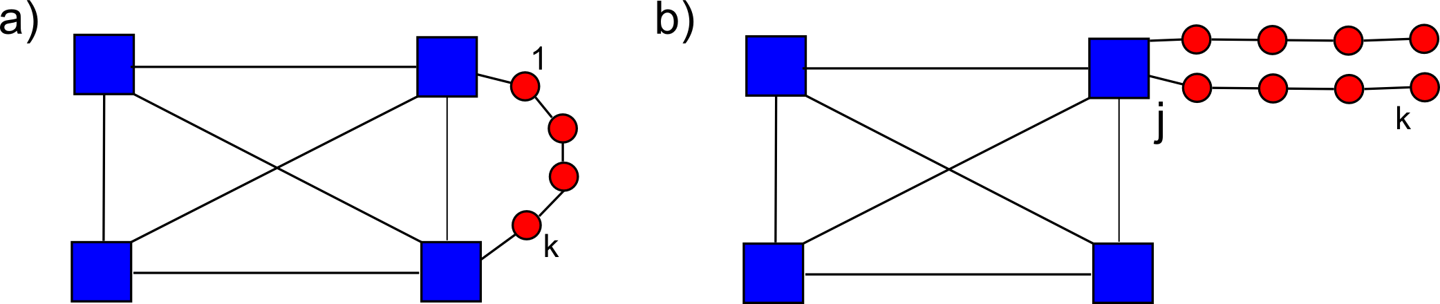
Figure 1: Non optimal networks. The type-A clique is in blue squares, the type-B players are in red circles. a) The network described in Example 8. b) A poor equilibrium, as described in the appendix.

Example 8.

Assume for simplicity that $c_{A}=c_{B}=c$. Consider a line of length $k$ of type B nodes, $(1,2,3...,k)$ such that $\sqrt{8c}>k+1>\sqrt{2c}$ or equivalently $\left(k+1\right)^{2}<8c<4\left(k+1\right)^{2}$ . In addition, the links $(j_{1},1)$ and $(j_{2},k)$ exist, where $j\in T_{A}$, i.e., the line is connected at both ends to different nodes of the type-A clique, as depicted in Fig 1. In [5] we show that this is a stabilizable graph.

A stable network cannot have two “heavy” trees, “heavy” here means that there is a deep sub-tree with many nodes, as it would be beneficial to make a shortcut between the two sub-trees(details appear in the appendix). In other words, trees must be shallow and small. This means that, while there are many equilibria, in all of them nodes cannot be too far apart, i.e., a small-world property. Furthermore, the trees formed are shallow and are not composed of many nodes.

3.3 Price of Anarchy & Price of Stability

As there are many possible link-stable equilibria, a discussion of the price of anarchy is in place. First, we explicitly find the optimal configuration. Although we establish a general expression for this configuration, it is worthy to also consider the limiting case of a large network, $|T_{B}|\gg 1,|T_{A}|\gg 1$. Moreover, typically, the number of major league players is much smaller than the other players, hence we also consider the limit $|T_{B}|\gg|T_{A}|\gg 1$.

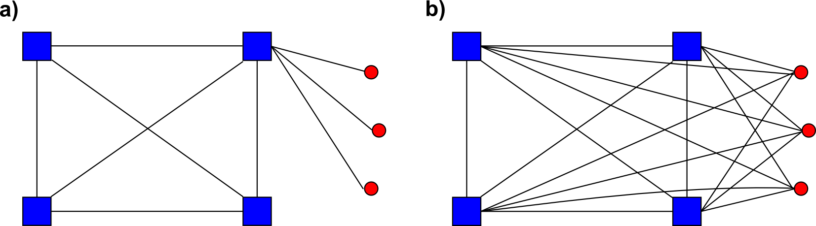
Figure 2: The optimal solution, as described in Lemma 9. If $\left(A+1\right)/2<c$ the optimal solution is described by a), otherwise by b). When monetary transfers (section 5) are allowed, both configurations are stabilizable. Otherwise, only a) is stabilizable.

Proposition 9.

Consider the network where the type $B$ nodes are connected to a specific node $j\in T_{A}$ of the type-A clique. The social cost in this stabilizable network (Fig. 2(a)) is

$$\mathcal{S} = 2|T_{B}|\left(|T_{B}|-1+c+\left(A+1\right)(|T_{A}|-1/2)\right)+|T_{A}|\left(|T_{A}|-1\right)\left(c_{A}+A\right).$$

Furthermore, if $|T_{B}|\gg 1,|T_{A}|\gg 1$ then, omitting linear terms in $|T_{B}|,|T_{A}|$,

$$\mathcal{S}=2|T_{B}|(|T_{B}|+\left(A+1\right)|T_{A}|)+|T_{A}|^{2}\left(c+A\right).$$

Moreover, if $\frac{A+1}{2}\leq c$ then this network structure is socially optimal and the price of stability is $1$, otherwise the price of stability is

$$PoS=\frac{2|T_{B}|(|T_{B}|+\left(A+1\right)|T_{A}|)+|T_{A}|^{2}\left(c_{A}+A\right)}{2|T_{B}|\left(|T_{B}|+\left(\frac{A+1}{2}+c\right)|T_{A}|\right)+|T_{A}|^{2}\left(c_{A}+A\right)}.$$

Finally, if $|T_{B}|\gg|T_{A}|\gg 1$, then the price of stability is asymptotically $1$.

Proof.

This structure is immune to removal of links as a disconnection of a $(type-B,type-A)$ link will disconnect the type-B node, and the type-A clique is stable (lemma 7). For every player $j$ and $i\in T_{B}$, any additional link $(i,j)$ will result in $\Delta C(j,E+ij)\geq c_{B}-1>0$ since the link only reduces the distance $d(i,j)$ from 2 to 1. Hence, player $j$ has no incentive to accept this link and no additional links will be formed. This concludes the stability proof.

We now turn to discuss the optimality of this network structure. First, consider a set of type-A players. Every link reduce the distance of at least two nodes by at least one, hence the social cost change by introducing a link is negative, since $2c_{A}-2A<0$. Therefore, in any optimal configuration the type-A nodes form a complete graph. The other terms in the social cost are due to the inter-connectivity of type-B nodes and the type-A to type-B connections. As $deg(i)=1$ for all $i\in T_{B}$ the cost due to link’s prices is minimal. Furthermore, $d(i,j)=1$ and the distance cost to node $j$ (of type A) is minimal as well. For all other nodes $j^{\prime}$, $d(i,j^{\prime})=2$.

Assume this configuration is not optimal. Then there is a topologically different configuration in which there exists an additional node $j^{\prime}\in T_{A}$ for which $d(i,j^{\prime})=1$ for some $i\in T_{B}$. Hence, there’s an additional link $(i,j)$. The social cost change is $2c+1+A$ . Therefore, if $\frac{A+1}{2}\leq c$ this link reduces the social cost. On the other hand, if $\frac{A+1}{2}>c$ every link connecting a type-B player to a type-A player improves the social cost, although the previous discussion show these link are unstable. In this case, the optimal configuration is where all type-B nodes are connected to all the type-A players, but there are no links linking type-B players. This concludes the optimality proof.

The cost due to inter-connectivity of type A nodes is

$$c_{A}|T_{A}|\left(|T_{A}|-1\right)+A|T_{A}|\left(|T_{A}|-1\right)=|T_{A}|\left(|T_{A}|-1\right)\left(c_{A}+A\right).$$

The first expression is due to the cost of $|T_{A}|$ clique’s links and the second is due to distance (=1) between each type-A node. The distance of each type B nodes to all the other nodes is exactly 2, except to node $j$, to which its distance is 1. Therefore the social cost due to type B nodes is

$$2|T_{B}|(|T_{B}|-1)+2c_{B}|T_{B}|+2\left(A+1\right)|T_{B}|\left(\left(|T_{A}|-1\right)+\left(A+1\right)+2\left(A+1\right)(|T_{A}|-1)\right)$$

$$= 2|T_{B}|\left(|T_{B}|-1+c_{B}+\left(A+1\right)(|T_{A}|-1/2)\right).$$

The terms on the left hand side are due to (from left to right) the distance between nodes of type B, the cost of each type-B’s single link, the cost of type-B nodes due to the distance (=2) to all member of the type-A clique bar $j$ and the cost of type $B$ nodes due to the distance (=1) to node $j$. The social cost is

$$\sum C(i) = 2|T_{B}|\left(|T_{B}|-1+c+\left(A+1\right)(|T_{A}|-1/2)\right)+|T_{A}|\left(|T_{A}|-1\right)\left(c_{A}+A\right).$$

To complete the proof, note that if $\frac{A+1}{2}>c$ the latter term in the social cost of the optimal (and unstable) solution is

$$2|T_{B}|(|T_{B}|-1)+2c|T_{B}|\left(1+|T_{A}|\right)+\left(A+1\right)|T_{B}||T_{A}|=2|T_{B}|\left(|T_{B}|-1+\left(\frac{A+1}{2}+c\right)|T_{A}|\right).$$

As the number of links is $|T_{B}|\left(1+|T_{A}|\right)$ and the distance of type-B to type-A nodes is 1. The optimal social cost is then

$$2|T_{B}|\left(|T_{B}|-1+\left(\frac{A+1}{2}+c\right)|T_{A}|\right)+|T_{A}|\left(|T_{A}|-1\right)\left(c_{A}+A\right).$$

Considering all quantities in the limit $|T_{B}|\gg|T_{A}|\gg 1$ completes the proof.∎

Next, we evaluate the price of anarchy. The social cost in the stabilizable topology presented in Fig 1, composed of a type-A clique and long lines of type-B players, is calculated in [5]. The ratio between this value and the optimal social cost constitutes a lower bound on the price of anarchy. An upper bound is obtained by examining the social cost in any topology that satisfies Lemma 7. The result in the large network limit is presented by the following proposition.

Proposition 10.

If $c_{B}<A$ and $|T_{B}|\gg|T_{A}|\gg 1$ the price of anarchy is $\Theta(c_{B})$.

4 Basic model - Dynamics

The Internet is a rapidly evolving network. In fact, it may very well be that it would never reach an equilibrium as ASs emerge, merge, and draft new contracts among them. Therefore, a dynamic analysis is a necessity. We first define the dynamic rules. Then, we analyze the basin of attractions of different states, indicating which final configurations are possible and what their likelihood is. We shall establish that reasonable dynamics converge to just a few equilibria. Lastly, we investigate the speed of convergence, and show that convergence time is linear in the number of players.

4.1 Setup & Definitions

At each point in time, the network is composed of a subset $N^{\prime}\subset T_{A}\cup T_{B}$ of players that already joined the game. The cost function is calculated with respect to the set of players that are present (including those that are joining) at the considered time. The game takes place at specific times, or turns, where at each turn only a single player is allowed to remove or initiate the formation of links. We split each turn into acts, at each of which a player either forms or removes a single link. A player’s turn is over when it has no incentive to perform additional acts.

Definition 11.

Dynamic Rule #1: In player $i$’s turn it may choose to act $m\in\mathcal{N}$ times. In each act, it may remove a link $(i,j)\in E$ or, if player $j$ agrees, it may establish the link $(i,j)$. Player $j$ would agree to establish $(i,j)$ iff $C(j;E+(i,j))-C(j;E)<0$.

The last part of the definition states that, during player’s $i$ turn, all the other players will act in a greedy, rather than strategic, manner. For example, although it may be that player $j$ prefers that a link $(i,j^{\prime})$ would be established for some $j^{\prime}\neq j$, if we adopt Dynamic Rule #1 it will accept the establishment of the less favorable link $(i,j).$ In other words, in a player’s turn, it has the advantage of initiation and the other players react to its offers. This is a reasonable setting when players cannot fully predict other players’ moves and offers, due to incomplete information [7] such as the unknown cost structure of other players. Another scenario that complies with this setting is when the system evolves rapidly and players cannot estimate the condition and actions of other players.

The next two rules consider the ratio of the time scale between performing the strategic plan and evaluation of costs. For example, can a player remove some links, disconnect itself from the graph, and then pose a credible threat? Or must it stay connected? Does renegotiating take place on the same time scale as the cost evaluation or on a much shorter one? The following rules address the two limits.

Definition 12.

Dynamic Rule #2a: Let the set of links at the current act $m$ be denoted as $E_{m}$. A link $(i,j)$ will be added if $i$ asks to form this link and $C(j;E_{m}+ij)<C(j;E_{m})$. In addition, any link $(i,j)$ can be removed in act $m.$

The alternative is as follows.

Definition 13.

Dynamic Rule #2b: In addition to Dynamic Rule #2a, player $i$ would only remove a link $(i,j)$ if $C(i;E_{m}-ij)>C(i;E_{m})$ and would establish a link if both $C(j;E_{m}+ij)<C(j;E_{m})$ and $C(i;E_{m}+ij)<C(i;E_{m})$.

The difference between the last two dynamic rules is that, according to Dynamic Rule #2a, a player may perform a strategic plan in which the first few steps will increase its cost, as long as when the plan is completed its cost will be reduced. On the other hand, according to Dynamic Rule #2b, its cost must be reduced at each act, hence such “grand plan” is not possible. Note that we do not need to discuss explicitly disconnections of several links, as these can be done unilaterally and hence iteratively.Finally, the following lemma will be useful in the next section.

Lemma 14.

Assume $N$ players act consecutively in a (uniformly) random order at integer times, which we’ll denote by $t$. the probability $P(t)$ that a specific player did not act $k\mathcal{\in N}$ times by $t\gg N$ decays exponentially.

4.2 Results

After mapping the possible dynamics, we are at a position to consider the different equilibria’s basins of attraction. Specifically, we shall establish that, in most settings, the system converges to the optimal network, and if not, then the network’s social cost is asymptotically equal to the optimal social cost. The main reason behind this result is the observation that a disconnected player has an immense bargaining power, and may force its optimal choice. As the highest connected node is usually the optimal communication partner for other nodes, new arrivals may force links between them and this node, forming a star-like structure. There may be few star centers in the graphs, but as one emerges from the other, the distance between them is small, yielding an optimal (or almost optimal) cost.

We outline the main ideas of the proof. The first few type-B players, in the absence of a type-A player, will form a star. The star center can be considered as a new type of player, with an intermediate importance, as presented in Fig. 3. We monitor the network state at any turn and show that the minor players are organized in two stars, one centered about a minor player and one centered about a major player (Fig. 3(a)). Some cross links may be present (Fig. 4). By increasing its client base, the incentive of a major player to establish a direct link with the star center is increased. This, in turn, increases the attractiveness of the star’s center in the eyes of minor players, creating a positive feedback loop. Additional links connecting it to all the major league players will be established, ending up with the star’s center transformation into a member of the type-A clique. On the other hand, if the star center is not attractive enough, then minor players may disconnect from it and establish direct links with the type-A clique, thus reducing its importance and establishing a negative feedback loop. The star will become empty, and the star’s center $x$ will be become a stub of a major player, like every other type-B player. The latter is the optimal configuration, according to proposition 9. We analyze the optimal choice of the active player, and establish that the optimal action of a minor player depends on the number of players in each structure and on the number of links between the major players and the minor players’ star center $x$. The latter figure depends, in turn, on the number of players in the star. We map this to a two dimensional dynamical system and inspect its stable points and basins of attraction of the aforementioned configurations.

Theorem 15.

If the game obeys Dynamic Rules #1 and #2a, then, in any playing order:

a) The system converges to a solution in which the total cost is at most

$$\mathcal{S} = |T_{A}|\left(|T_{A}|-1\right)\left(c+A\right)+2c_{B}|T_{B}|+\left(A+1\right)\left(3|T_{A}||T_{B}|-|T_{A}|+|T_{B}|\right)+2\left(|T_{B}|-1\right)^{2};$$

furthermore, by taking the large network limit $|T_{B}|\gg|T_{A}|\gg 1$, we have $\mathcal{S}/\mathcal{S}_{optimal}\rightarrow 1$ .

b) Convergence to the optimal stable solution occurs if either:

1) $A\cdot k_{A}>k+1$, where $k\geq 0$ is the number of type-B nodes that first join the network, followed later by $k_{A}$ consecutive type-A nodes (“initial condition”).

2)$A\cdot|T_{A}|>|T_{B}|$ (“final condition”).

c) In all of the above, if every player plays at least once in O(N) turns, convergence occurs after O(N) steps. Otherwise, if players play in a uniformly random order, the probability the system has not converged by turn $t$ decays exponentially with $t$.

Proof.

Assume $c_{A}\geq 2$. Denote the first type-A player that establish a link with a type-B player as $k$. First, we show that the network structure is composed of a type-A (possibly empty) clique, a set of type-B players $S$ linked to player $x$, and an additional (possibly empty) set of type-B players $L$ connected to the type-A player $k$. See Fig. 3(a) for an illustration. In addition, there is a set $D$ type-A nodes that are connected to node $x$, the star center. After we establish this, we show that the system can be mapped to a two dimensional dynamical system. Then, we evaluate the social cost at each equilibria, and calculate the convergence rate. We assume $(k,x)\in E$ and discuss the case $(k,x)\notin E$ in the appendix.

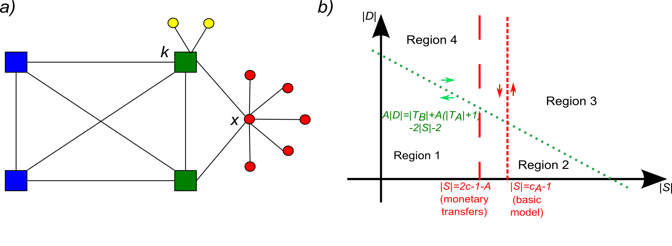
Figure 3: a) The network structures described in Theorem 15. The type-A clique contains $|T_{A}|=4$ nodes (squares), and there are $|S|=5$ nodes in the star (red circles). There are $|L|=2$ nodes that are connected directly to node $k$ (yellow circles). The number of type-A nodes that are connected to node 1, the star center, is $|D|=2$ (green squares). b) The phase state of Theorem 15. The dotted green line is the $|S|$ increase / decrease nullcline. The dotted (dashed) red line is the nullcline for the increase / decrease in $|D|$ when monetary transfers are forbidden (allowed). (Proposition 24).

We prove by induction. At turn $t\leq 2$, after the first two players joined the network, this is certainly true. Denote the active player at time $t$ as $r.$ Consider the following cases:

1. $r\in T_{A}$: Since $1<c_{A}<A,$ all links to the other type-A nodes will be established (lemma 9) or maintained, if $r$ is already connected to the network. Clearly, the optimal link in $r$’s concern is the link with star center $x$. As $c_{B}<A$ every minor player will accept a link with a major player even if it reduces its distance only by one. Therefore, the link $(r,x)$ is formed if the change of cost of the major player $r$,

$$\Delta C(r,E+rx)=c_{A}-|S|-1$$ (1)

is negative. In this case, the number of type A players connected to the star’s center, $|D|$, will increase by one. If this expression is positive and player $r$ is connected to at least another major player (as otherwise the graph is disconnected), the link will be dissolved and $|D|$ will be reduced by one. It is not beneficial for $r$ to form an additional link to any type-B player, as they only reduce the distance from a single node by one (see the discussion in lemma 9 in the appendix).

2. $r\in T_{B},\,r\neq x$ : First, assume that $r$ is a newly arrived player, and hence it is disconnected. Obviously, in its concern, a link to the star’s center, player $x$, is preferred over a link to any other type-B player. Similarly, a link to a type-A player that is linked with the star’s center is preferred over a link with a player that maintains no such link.

We claim that either $(r,k)$ or $(r,x)$ exists. Denote the number of type-A player at turn $t$ as $m_{A}.$ The link $(r,x)$ is preferred in $r$’s concern if the expression

$$C(r,E+rk)-C(r,E+rx)=-A(1+m_{A}-|D|)+1+|S|-|L|$$ (2)

is positive, and will be established as otherwise the network is disconnected. If the latter expression is negative, $(r,k)$ will be formed. The same reasoning as in case 1 shows that no additional links to a type-B player will be formed. Otherwise, if $r$ is already connected to the graph, than according to Dynamic Rule #2a, $r$ may disconnect itself, and apply its optimal policy, increasing or decreasing $|L|$ and $|S|$.

3. $r=x$, the star’s center: $r$ may not remove any edge connected to a type-B player and render the graph disconnected. On the other hand, it has no interest in removing links to major players. On the contrary, it will try to establish links with the major players, and these will be formed if eq. 1 is negative. An additional link to a minor player connected to $k$ will only reduce the distance to it by one and since $c_{B}>2$ player $x$ would not consider this move worthy.

The dynamical parameters that govern the system dynamics are the number of players in the different sets, $|S|$, $|L|$, and $|D|$. Consider the state of the system after all the players have player once. Using the relations $|S|+|L|+1=|T_{B}|,\>m_{A}=|T_{A}|$ we note the change in $|S|$ depends on $|S|$ and $|L|$ while the change in $|D|$ depends only on $|S|.$ We can map this to a 2D dynamical, discrete system with the aforementioned mapping. In Fig. 3 the state is mapped to a point in phase space $(|S|,|L|)$. The possible states lie on a grid, and during the game the state move by an single unit either along the $x$ or $y$ axis. There are only two stable points, corresponding to $|S|=0,|D|=1$, which is the optimal solution (Fig. 2(a)), and the state $|S|=|T_{B}|-1$ and $|D|=|T_{A}|$.

If at a certain time expression 1 is positive and expression 2 is negative (region 3 in Fig. 3(b)), the type-B players will prefer to connect to player $x$. This, in turn, increases the benefit a major player gains by establishing a link with player $x.$ The greater the set of type-A that have a direct connection with $x$, having $|D|$ members, the more utility a direct link with $x$ carries to a minor player. Hence, a positive feedback loop is established. The end result is that all the players will form a link with $x$. In particular, the type-A clique is extended to include the type-B player $x$. Likewise, if the reverse condition applies, a feedback loop will disconnect all links between node $x$ to the clique (except node $k$) and all type-B players will prefer to establish a direct link with the clique. The end result in this case is the optimal stable state. The region that is relevant to the latter domain is region 1.

However, there is an intermediate range of states, described by region 2 and region 4, in which the player order may dictate to which one of the previous states the system will converge. For example, starting from a point in region 4, if the type-A players move first, changing the $|D|$ value, than the dynamics will lead to region 1, which converge to the optimal solution. However, if the type-B players move first, then the system will converge to the other equilibrium point.

We now turn to calculate the social cost at the different equilibria. If $|D|=|T_{A}|$ and $|S|=|T^{\prime}_{B}|-1$, The network topology is composed of a $|T_{A}|$ members clique, all connected to the center $x$, that, in turn, has $|T_{B}|-1$ stubs. The total cost in this configuration is

$$S = |T_{A}|\left(|T_{A}|-1\right)\left(c_{A}+A\right)+2c_{B}|T_{B}|+\left(A+1\right)|T_{A}|+2\left(|T_{B}|-1\right)$$ (3)

$$+2\left(|T_{B}|-1\right)\left(A+1\right)+2\left(|T_{B}|-2\right)\left(|T_{B}|-1\right)+\left(c_{B}+c_{A}\right)|T_{A}|/2$$

where the costs are, from the left to right: the cost of the type-A clique, the cost of the type-B star’s links, the distance cost $(=1)$ between the clique and node $x$, the distance $(=1)$ cost between the star’s members and node $x$, the distance $(=2)$ cost between the clique and the star’s member, the distance $(=2)$ cost between the star’s members, and the cost due to major player link’s to the start center $x$. Adding all up, we have for the total cost

$$\mathcal{S} \leq |T_{A}|\left(|T_{A}|-1\right)\left(c+A\right)+2c_{B}|T_{B}|+\left(A+1\right)\left(3|T_{A}||T_{B}|+|T_{B}|\right)+2\left(|T_{B}|-1\right)^{2}.$$ (4)

Convergence is fast, and as soon as all players have acted three times the system will reach equilibrium. If every player plays at least once in $o(N$) turns convergence occurs after $o(N)$ turns, otherwise the probability the system did not reach equilibrium by time $t$ decays exponentially with $t$ according to lemma 14 (in the appendix).

We now relax our previous assumption $c_{A}\geq 2$. If $c_{A}\leq 2$ and the active player $r\in T_{A}$ then it will form a link with the star’s center according to eq. 1. If $r\in S$ it may establish a link $(r,j)$ with a type A player, which will later be replaced, in $j$’s turn, with the link $(j,x)$ according to the previous discussion. In the appendix we discuss explicitly the case where $(k,x)\notin E$ and show that in this case, additional links may be formed, e.g., a link between one of $k^{\prime}$s stubs, $i\in L$, and the star’s center $x$, as presented in Fig. 4. These links only reduce the social cost, and do not change the dynamics, and the system will converge to either one of the aforementioned states. Taking the limit $T_{B}\rightarrow\infty$ and $T_{B}\in\omega\left(T_{A}\right)$ in eq. 4, we get $\mathcal{S}/\mathcal{S}_{optimal}\rightarrow 1$. This concludes the proof.

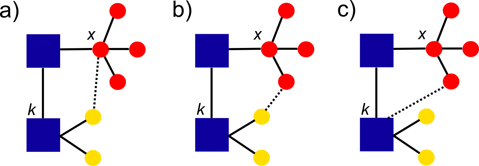
Figure 4: Additional feasible cross-tiers links, as described in Meirom et al. [5]. The star players $S$ are in red, the set $L$ is in yellow. a) a link between the star center and $i\in L$. b) a cross-tier link $(i,j)$ where $i\in S,j\in L$. c) a minor player - major player link, $(i,j)$ where $i\in T_{A}$ and $j\in S.$

∎

If the star’s center has a principal role in the network, then links connecting it to all the major league players will be established, ending up with the star’s center transformation into a member of the type-A clique. This dynamic process shows how an effectively new major player emerges out of former type-B members in a natural way. Interestingly, Theorem 15 also shows that there exists a transient state with a better social cost than the final state. In fact, in a certain scenario, the transient state is better than the optimal stable state.

So far we have discussed the possibility that a player may perform a strategic plan, implemented by Dynamic Rule #2a. However, if we follow Dynamic Rule #2b instead, then a player may not disconnect itself from the graph. The previous results indicate that it is not worthy to add additional links to the forest of type-B nodes. Therefore, no links will be added except for the initial ones, or, in other words, renegotiation will always fail. The dynamics will halt as soon as each player has acted once. Formally:

Proposition 16.

If the game obeys Dynamic Rules #1 and #2b, then the system will converge to a solution in which the total cost is at most

$$\mathcal{S} = |T_{A}|\left(|T_{A}|-1\right)\left(c_{A}+A\right)+3|T_{B}|^{2}+2c_{B}|T_{B}|+2|T_{A}||T_{B}|\left(A+1\right)\,.$$

Furthermore, for $|T_{B}|\gg|T_{A}|\gg 1$, we have $\mathcal{S}/\mathcal{S}_{optimal}\leq 3/2.$ Moreover, if every player plays at least once in O(N) turns, convergence occurs after O(N) steps. Otherwise, if players play in a uniformly random order, the probability the system has not converged by turn $t$ decays exponentially with $t$.

Proof.

We discuss the case $c_{A}\geq 2.$ The extension for $c_{A}<2$ appears in the appendix. The first part of the proof follows the same lines of the previous theorem (Theorem 15). We claim that at any given turn, the network structure is composed of the same structures as before (See Fig. 3(a)) . Here, we discuss the scenario where $(k,x)\in E,$ and we address the other possibility, which may give rise to the structures shown in Fig. 4 in the appendix.

We prove by induction. Clearly, at turn one the induction assumption is true. Note that for newly arrived players, are not affected by either Dynamic Rules #2a or #2b. Hence, we only need to discuss the change in policies of existing players. The only difference from the dynamics described in the Theorem 15 is that the a type-B players may not disconnect itself. In this case, as the discussion there indicates the star center $x$ will refuse a link with $i\in L$ as it only reduce $d(i,x)$ by two. Equivalently, $k$ will refuse to establish additional links with $i\in|S|.$

In other words, as soon the first batch of type A player arrives, all type-B players will become stagnant, either they become leaves of either node $k$, $|L|$, or members of the star $|S|$, according to the the sign of 2 at the time they. The maximal distance between a type-A player and a type B player is $2$. The maximal value of the type B - type B term is the social cost function is when $|L|=|S|=|T_{B}|/2$. In this case, this term contributes $3|T_{B}|^{2}$ to the social cost. Therefore, the social cost is bounded by

$$\mathcal{S}=|T_{A}|\left(|T_{A}|-1\right)\left(c_{A}+A\right)+3|T_{B}|^{2}+2c_{B}|T_{B}|+2|T_{A}||T_{B}|\left(A+1\right)$$ (5)

where we included the type-A clique’s contribution to the social cost and used $c_{B}\geq c_{A}.$ Taking the limit $N\rightarrow\infty$ in eq. 5 and using $T_{A}\in\omega(1)$, $T_{B}\in\omega(T_{A})$, we obtain $\mathcal{S}/\mathcal{S}_{optimal}\leq 3/2$. ∎

Theorem 15 and Proposition 16 shows that the intermediate network structures of the type-B players are not necessarily trees, and additional links among the tier two players may exist, as found in reality. Furthermore, our model predicts that some cross-tier links, although less likely, may be formed as well. If Dynamic Rule #2a is in effect, These structures are only transient, otherwise they might remain permanent.

The dynamical model can be easily generalized to accommodate various constraints. Geographical constraints may limit the service providers of the minor player. The resulting type-B structures represent different geographical regions. Likewise, in remote locations state legislation may regulate the Internet infrastructure. If at some point regulation is relaxed, it can be modeled by new players that suddenly join the game.

5 Monetary transfers

So far we assumed that a player cannot compensate other players for an increase in their costs. However, contracts between different ASs often do involve monetary transfers. Accordingly, we turn to consider the effects of introducing such an option on the findings presented in the previous sections. As before, we first consider the static perspective and then turn to the dynamic perspective.

5.1 Statics

In the previous sections we showed that, if $A>c_{A}>1,$ then it is beneficial for each type-A player to be connected to all other type-A players. We focus on this case.

Monetary transfers allow for a redistribution of costs. It is well known in the game theoretic literature that, in general, this process increases the social welfare.Indeed, the next proposition indicates an improvement on Proposition 9. Specifically, it shows that the optimal network is always stabilizable, even when $\frac{A+1}{2}>c$. Without monetary transfers, the additional links in the optimal state (Fig. 2), connecting a major league player with a minor league player, are unstable as the type-A players lack any incentive to form them. By allowing monetary transfers, the minor players can compensate the major players for the increase in their costs. It is worthwhile to do so only if the social optimum of the two-player game implies it. The existence or removal of an additional link does not inflict on any other player, as the distance between every two players is at most two.

Proposition 17.

The price of stability is $1$. If $\frac{A+1}{2}\leq c\,,$ then Proposition 9 holds. Furthermore, if $\frac{A+1}{2}>c$, then the optimal stable state is such that all the type $B$ nodes are connected to all nodes of the type-A clique. In the latter case, the social cost of this stabilizable network is $\mathcal{S}=2|T_{B}|\left(|T_{B}|+\left(\frac{A+1}{2}+c\right)|T_{A}|\right)+|T_{A}|^{2}\left(c+A\right).$ Furthermore, if $|T_{B}|\gg 1,|T_{A}|\gg 1$ then, omitting linear terms in $|T_{B}|,|T_{A}|$, $\mathcal{S}=2|T_{B}|(|T_{B}|+\left(A+c\right)|T_{A}|)+|T_{A}|^{2}\left(c+A\right).$

In the network described by Fig. 2, the minor players are connected to multiple type-A players. This emergent behavior, where ASs have multiple uplink-downlink but very few (if at all) cross-tier links, is found in many intermediate tiers.

Next, we show that, under mild conditions on the number of type-A nodes, the price of anarchy is $3/2$, i.e., a fixed number that does not depend on any parameter value. As the number of major players increases, the motivation to establish a direct connection to a clique member increases, since such a link reduces the distance to all clique members. As the incentive increases, players are willing to pay more for this link, thus increasing, in turn, the utility of the link in a major player’s perspective. With enough major players, all the minor players will establish direct links. Therefore, any stable equilibrium will result in a very compact network with a diameter of at most three. This is the main idea behind the following theorem.

Theorem 18.

The maximal distance of a type-B node from a node in the type-A clique is $\max\left\{\left\lfloor\sqrt{\left(A|T_{A}|\right)^{2}+4cA|T_{A}|}-A|T_{A}|\right\rfloor,2\right\}$. Moreover, if $|T_{B}|\gg 1,|T_{A}|\gg 1$ then the price of anarchy is upper-bounded by 3/2.

This theorem shows that by allowing monetary transfers, the maximal distance of a type-B player to the type-A clique depends inversely on the number of nodes in the clique and the number of players in general. The number of ASs increases in time, and we may assume the number of type-A players follows. Therefore, we expect a decrease of the mean “node-core distance” in time. Our data analysis, which appears in the appendix, indicates that this real-world distance indeed decreases in time.

5.2 Dynamics

We now consider the dynamic process of network formation under the presence of monetary transfers. For every node $i$ there may be several nodes, indexed by j, such that $\Delta C(j,ij)+\Delta C(i,ij)<0,$ and player i needs to decide on the order of players with which it will ask to form links. We point out that the order of establishing links is potentially important. The order by which player player $i$ will establish links depends on the pricing mechanism. There are several alternatives and, correspondingly, several possible ways to specify player i’s preferences, each leading to a different dynamic rule.

Perhaps the most naive assumption is that if for player $j,$ $\Delta C(j,ij)>0$, then the price it will ask player $i$ to pay is $P_{ij}=\max\{\Delta C(j,ij),0\}.$ In other words, if it is beneficial for player $j$ to establish a link, it will not ask for a payment in order to do so. Otherwise, it will demand the minimal price that compensates for the increase in its costs. This dynamic rule represents an efficient market. This suggests the following preference order rule.

Definition 19.

Preference Order #1: Player $i$ will establish a link with a player $j$ such that $\Delta C(i,ij)+min\{\Delta C(j,ij),0\}$ is minimal. The price player $i$ will pay is $P_{ij}=max\{\Delta C(j,ij),0\}$.

As established by the next theorem, Preference Order #1 leads to the optimal equilibrium fast. In essence, if the clique is large enough, then it is worthy for type-B players to establish a direct link to the clique, compensating a type-A player, and follow this move by disconnecting from the star. Therefore, monetary transfers increase the fluidity of the system, enabling players to escape from an unfortunate position. Hence, we obtain an improved version of Theorem 15.

Theorem 20.

Assume the players follow Preference Order #1 and Dynamic Rule #1, and either Dynamic Rule #2a or #2b. If $\frac{A+1}{2}>c$, then the system converges to the optimal solution. If every player plays at least once in O(N) turns, convergence occurs after o(N) steps. Otherwise, e.g., if players play in a random order, convergence occurs exponentially fast.

Yet, the common wisdom that monetary transfers, or utility transfers in general, should increase the social welfare, is contradicted in our setting by the following proposition. Specifically, there are certain instances, where allowing monetary transfers yields a decrease in the social utility. In other words, if monetary transfers are allowed, then the system may converge to a sub-optimal state.

Proposition 21.

Assume $\frac{A+1}{2}\leq c$. Consider the case where monetary transfers are allowed and the game obeys Dynamic Rules #1,#2a and Preference Order #1. Then:

a) The system will either converge to the optimal solution or to a solution in which the social cost is

$$\mathcal{S} = |T_{A}|\left(|T_{A}|-1\right)\left(c_{A}+A\right)+2\left(|T_{B}|-1\right)^{2}+\left(A+1\right)\left(3|T_{A}||T_{B}|-|T_{A}|+|T_{B}|\right)+2c|T_{B}|.$$

For $|T_{B}|\rightarrow\infty$, $|T_{B}|\in\omega\left(|T_{A}|\right)$ we have $S/S_{optimal}\rightarrow 1\,$. In addition, if one of the first $\left\lfloor c-1\right\rfloor$ nodes to attach to the network is of type-A then the system converges to the optimal solution.

b) For some parameters and playing orders, the system converges to the optimal state if monetary transfers are forbidden, but when transfers are allowed it fails to do so. This is the case, for example, when the first $k$ players are of type-B, and $2c-A-1<k<c-1$.

Proof.

a) We claim that, at any given turn $t$, the network is composed of the same structures as in Theorem 15. We use the notation described there. See Fig. 3 for an illustration. We assume that the link $(k,x)$ exists and elaborate in the appendix on the scenario that, at some point, the link $(k,x)$ is removed.

We prove by induction. At turn $t=1$ the induction hypothesis is true. We’ll discuss the different configurations at time $t$.

1. $r\in T_{A}$: As before, all links to the other type-A nodes will be established or maintained, if $r$ is already connected to the network. The link $(r,x)$ will be formed if the change of cost of player $r$,

$$\Delta C(r,E+rx)+\Delta C(x,E+rx)=2c-A-|S|-1$$ (6)

is negative. In this case $|S|$ will increase by one. If this expression is positive and $(r,x)\in E,$ the link will be dissolved and $|D|$ will be reduced. It is not beneficial for $r$ to form an additional link to any type-B player, as they only reduce the distance from a single node by 1 and $\frac{A+1}{2}\leq c$.

2. $r\in T_{B}$ :The discussion in Theorem 15 shows that a newly arrived may choose to establish its optimal link, which would be either $(r,k)$ or $(r,x)$ according to the sign of expression 2. As otherwise the graph is disconnected, such link will cost nothing. Similarly, if $r$ is already connected, it may disconnect itself as an intermediate state and use its improved bargaining point to impose its optimal choice. Hence, the formation of either $(r,k)$ or $(r,x)$ is not affected by the inclusion of monetary transfers to the basic model. Assume the optimal move for $r$ is to be a member of the star, $r\in S$. If $\Delta C(k,E+kr)+\Delta C(r,E+kr)=2c-A|m_{A}|-1-|L|$ is negative, than this link will be formed. In this case, $r$ is a member of both $S$ and $L$, and we address this by the transformation $|S|\leftarrow|S|$, $|L|\leftarrow|L|+1$ and $|T_{B}|\leftarrow|T_{B}|+1.$ Similarly, if $r\in L$ than it will establish links with the star center $x$ if and only if $2c<|S|+1$. The analogous transformation is, $|S|\leftarrow|S|+1$, $|L|\leftarrow|L|$ and $|T_{B}|\leftarrow|T_{B}|+1.$ The rest of the proof follows along the lines of Theorem 15 and is detailed in the appendix.

b) If dynamic rule #2a is in effect, the nullcline represented by eq. 6 is shifted to the left compared to the nullcline of eq. 1, increasing region 3 and region 2 on the expanse of region 1 and region 4. Therefore, there are cases where the system would have converge to the optimal state, but allowing monetary transfers it would converge to the other stable state. Intuitively, the star center may pay type-A players to establish links with her, reducing the motivation for one of her leafs to defect and in turn, increasing the incentive of the other players to directly connect to it. Hence, monetary transfers reduce the threshold for the positive feedback loop discussing in Theorem 15.∎

The latter proposition shows that the emergence of an effectively new major league player, namely the star center, occurs more frequently with monetary transfers, although the social cost is hindered.

A more elaborate choice of a price mechanism is that of “strategic” pricing. Specifically, consider a player $j^{*}$ that knows that the link $(i,j^{*})$ carries the least utility for player $i$. It is reasonable to assume that player $j$ will ask the minimal price for it, as long as it is greater than its implied costs. We will denote this price as $P_{ij^{*}}$. Every other player $x$ will use this value and demand an additional payment from player $i$, as the link $(i,x)$ is more beneficial for player $i$. Formally,

Definition 22.

Pricing mechanism #2: Set $j^{*}$ as the node that maximizes $\Delta C(i,E+ij*)$. Set $P_{ij^{*}}=\max\{-\Delta C(j*,E,ij*),0\}$. Finally, set $\alpha_{ij}=\Delta C(i,E+ij)-\left(\Delta C(i,E+ij^{*})+P_{ij^{*}}\right).$ The price that player $j$ requires in order to establish $(i,j)$ is $P_{ij}=\max\{0,\alpha_{ij},-\Delta C(j,E+ij)\}$.

As far as player $i$ is concerned, all the links $(i,j)$ with $P_{ij}=\alpha_{ij}$ carry the same utility, and this utility is greater than the utility of links for which the former condition is not valid. Some of these links have a better connection value, but they come at a higher price. Since all the links carry the same utility, we need to decide on some preference mechanism for player $i$. The simplest one is the “cheap” choice, by which we mean that, if there are a few equivalent links, then the player will choose the cheapest one. This can be reasoned by the assumption that a new player cannot spend too much resources, and therefore it will choose the “cheapest” option that belongs to the set of links with maximal utility.

Definition 23.

Preference order #2: Player $i$ will establish links with player $j$ if player $j$ minimizes $\Delta\tilde{C}(i,ij)=\Delta C(i,ij)+P_{ij}$ and $\Delta\tilde{C}(i,ij)<0$.

If there are several players that minimize $\Delta\tilde{C}(i,ij)$, then player $i$ will establish a link with a player that minimizes $P_{ij}$. If there are several players that satisfy the previous condition, then one out of them is chosen randomly.

Note that low-cost links have a poor “connection value” and therefore the previous statement can also be formulated as a preference for links with low connection value.

We proceed to consider the dynamic aspects of the system under such conditions.

Proposition 24.

Assume that:

A) Players follow Preference Order #2 and Dynamic Rule #1, and either Dynamic Rule #2a or #2b.

B) There are enough players such that $2c<T_{A}\cdot A+T_{B}^{2}/4$.

C) At least one out of the first $m$ players is of type-A, where $m$ satisfies $m\geq\sqrt{A^{2}+4c-1}-A$.

Then, if the players play in a non-random order, the system converges to a state where all the type-B nodes are connected directly to the type-A clique, except perhaps lines of nodes with summed maximal length of $m$. In the large network limit, $\mathcal{S}/\mathcal{S}_{optimal}<3/2+c$ .

D) If $2c>(A-1)+|T_{B}|/|T_{A}|$ then the bound in (C) can be tightened to $\mathcal{S}/\mathcal{S}_{optimal}<3/2$.

In order to obtain the result in Proposition 18, we had to assume a large limit for the number of type-A players. Here, on the other hand, we were able to obtain a similar result yet without that assumption, i.e., solely by dynamic considerations.

It is important to note that, although our model allows for monetary transfers, in every resulting agreement between major players no monetary transaction is performed. In other words, our model predicts that the major players clique will form a settlement-free interconnection subgraph, while in major player - minor player contracts transactions will occur, and they will be of a transit contract type. Indeed, this observation is well founded in reality.

6 Conclusions

Does the Internet resembles a clique or a tree? Is it contracting or expanding? Can one statement be true on one segment of the network while the opposite is correct on a different segment? The game theoretic model presented in this work, while abstracting many details away, focuses on the essence of the strategical decision-making that ASs perform. It provides answers to such questions by addressing the different roles ASs play.

The static analysis has indicated that in all equilibria, the major players form a clique. Our model predicts that the major players clique will form a settlement-free interconnection subgraph, while in major player - minor player contracts transactions will occur, and they will be of a transit contract type. This observation is supported by the empirical evidence,showing the tight tier-1 subgraph, and the fact these ASs provide transit service to the other ASs.

We discussed multiple dynamics, which represent different scenarios and playing orders. The dynamic analysis showed that, when the individual players act selfishly and rationally, the system will converge to either the optimal configuration or to a state in which the social cost differs by a negligible amount from the optimal social cost. This is important as a prospective mechanism design. Furthermore, although a multitude of equilibria exist, the dynamics restrict the convergence to a limited set. In this set, the minor players’ dominating structures are lines and stars. We also learned that, as the number of major players increase, the distance of the minor players to the core should decrease. This theoretical finding was also confirmed empirically (see the appendix).

In our model, ASs are lumped into two categories. The extrapolation of our model to a general (multi-tier) distribution of player importance is an interesting and relevant future research question, the buds of which are discussed in the appendix. In addition, there are numerous contract types (e.g., p2p, customer-to-provider, s2s) ASs may form. While we discussed a network formed by the main type (c2p), the effect of including various contract types is yet to be explored.

Appendix A Appendix: Data analysis

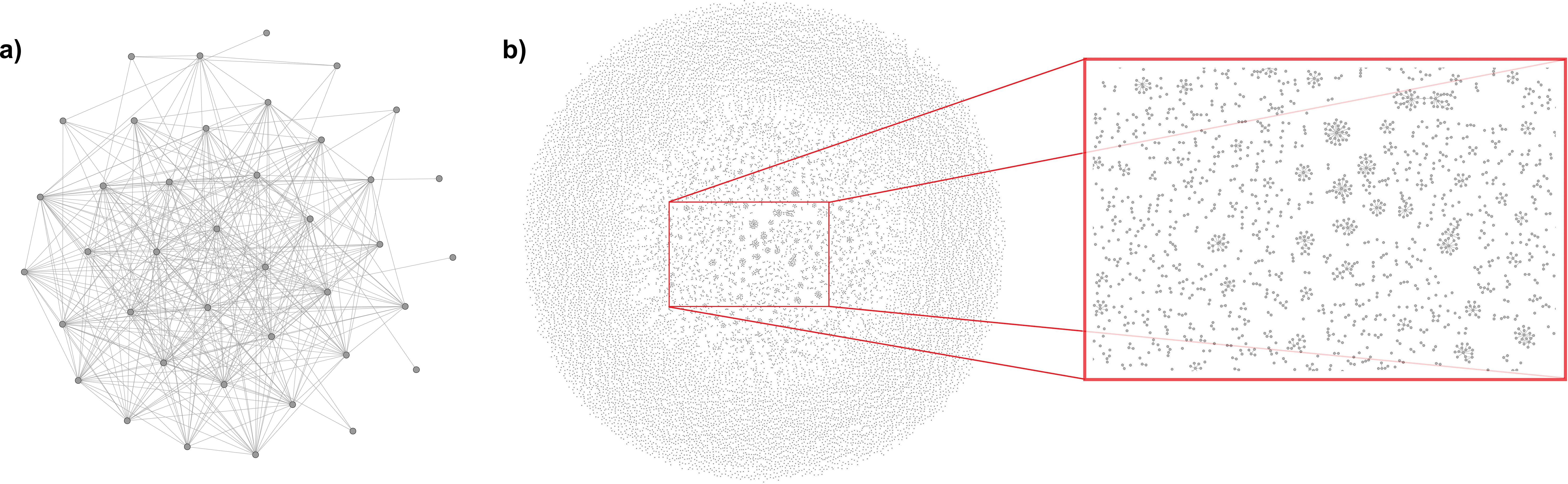
Figure 5: Structure of the AS topology. a) The sub-graph of the top 40 ASs, according to CAIDA ranking, in January, 2006. b) The minor nodes sub-graph was created by omitting nodes in higher k-core $(k\geq 3$) and removing any links from the shell to the core. The subgraph contains 16,442 nodes, which are $\sim 75\%$ of the ASs in the networks. Left: The full network map. Singleton are displayed in the exterior and complex objects in the center. Right: A zoom-in on a sample (red box) of the subgraph. The complex structure are mainly short lines and stars (or star-like objects).

As discussed in the Introduction, the Internet is composed of autonomous subsystems, each we consider to be a player. It is one particular case to which our model can be applied, and in fact it has served as the main motivation for our study. Accordingly, in this appendix we compare our theoretical findings with actual monthly snapshots of the inter-AS connectivity, reconstructed from BGP update messages Gregori2011.

Our model predicts that, for $A>c>1$ , the type-A (“major league”) players will form a highly connected subset, specifically a clique (Section 3.1). The type-B players, in turn, form structures that are connected to the clique. Figure 5 presents the graph of a subset of the top 100 ASs per January 2006, according to CAIDA ranking CAIDA. It is visually clear that the inter-connectivity of this subset is high. Indeed, the top 100 ASs graph density, which is the ratio between the number of links present and the number of possible links, is 0.23, compared to a mean $0.024\pm 0.004$ for a random connected set of 100. It is important to note that we were able to obtain similar results by ranking the top ASs using topological measures, such as betweeness, closeness and k-core analysis Meirom2013 .

Although, in principle, there are many structures the type-B players (“minor players”) may form, the dynamics we considered indicates the presence of stars and lines mainly (Sections 4.2 and 5.2). While the partition of ASs to just two types is a simplification, we still expect our model to predict fairly accurately the structures at the limits of high-importance ASs and marginal ASs. A $k$-core of a graph is the maximal connected subgraph in which all nodes have degree of at least $k$. The $k$-shell is obtained after the removal of all the $k$-core nodes. In Fig. 5, a snapshot of the sub-graph of the marginal ASs is presented, using a $k$-core separation ($k=3$), where all the nodes in the higher cores are removed. The abundance of lines and stars is visually clear. In addition, the spanning tree of this subset, which consists of 75% of the ASs in the Internet, is formed by removing just 0.02% of the links in this sub-graph, a strong indication for a forest-like structure.

In the dynamic aspect, we expect the type-A players sub-graph to converge to a complete graph. We evaluate the mean node-to-node distance in this subset as a function of time by using quarterly snapshots of the AS graph from January, 2006 to October, 2008. Indeed, the mean distance decreases approximately linearly. The result is presented in Fig. 6. Also, the distance value tends to $1$, indicating the almost-completeness of this sub-graph.

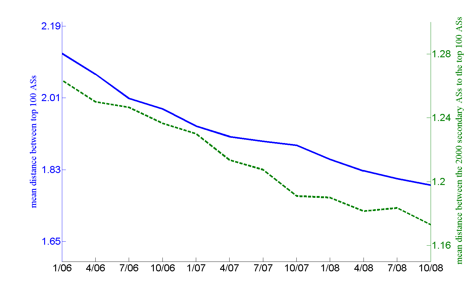
Figure 6: In solid blue: the mean distance of an AS in the top 100 ASs CAIDA ranking to all the other top 100 ASs, from January, 2006 to October, 2008. In dashed green: The mean shortest distance of a secondary AS (ranked 101-2100) from any top AS (ranked 1-100).

For a choice of core $\mathcal{C}$, the node-core distance of a node $i\notin\mathcal{C}$ is defined as the shortest path from node $i$ to any node in the core. In Section 5, we showed that, by allowing monetary transfers, the maximal distance of a type-B player to the type-A clique (the maximal “node-core distance” in our model) depends inversely on the number of nodes in the clique and the number of players in general. Likewise, we expect the mean “node-core” distance to depend inversely on the number of nodes in the clique. The number of ASs increases in time, and we may assume the number of type-A players follows. Therefore, we expect a decrease of the aforementioned mean “node-core distance” in time. Fig 6 shows the mean distance of the secondary leading 2000 ASs, ranked 101-2100 in CAIDA ranking, from the set of the top 100 nodes. The distance decreases in time, in agreement with our model. Furthermore, our dynamics indicate that the type-B nodes would be organized in stars, for which the mean “node-core” distance is close to two, and in singleton trees, for which the “node-core” distance is one. Indeed, as predicted, the mean “node-core” distance proves to be between one and two.

It is widely assumed that the evolvement of the Internet follows a “preferential attachment” process Barabasi1999. According to this process, the probability that a new node will attach to an existing node is proportional (in some models, up to some power) to the existing node’s degree. An immediate corollary is that the probability that a new node will connect to any node in a set of nodes is proportional to the set’s sum of degrees. The sum of degrees of the secondary ASs set is ~1.9 greater than the sum of degrees in the core, according to the examined data Gregori2011. Therefore, a “preferential attachment” class model predicts that a new node is likely to attach to the shell rather than to the core. As all the nodes in the shell have a distance of at least one from the core, the new node’s distance from the core will be at least two. Since the initial mean “shell-core” distance is ~1.26, a model belonging to the “preferential attachment” class predicts that the mean distance will be pushed to two, and in general increase over time. However, this is contradicted by the data that shows (Fig 6) a decrease of the aforementioned distance. The slope of the latter has the 95% confidence bound of $(-3.1\cdot 10^{-3},-2.3\cdot 10^{-3}$) hops/month, a strong indication of a negative trend, in disagreement with the “preferential attachment” model class. In contrast, this trend is predicted by our model, per the discussion in Section 5. In fact, if the Internet is described by a random, power law (“scale free”) network, then the mean distance should grow as $\Theta(\log N)$ or $\Theta(\log\log N)$ (Cohen2003). However, experimental observations shows that the mean distance grows slower than that (Pastor-Satorras2001 ), and it fact it may even be reduced with the network size, as predicted by our model.

Appendix B Appendix : Detailed proofs

B.1 Basic model - Static Analysis

In this section we discuss the properties of stable equilibria. Specifically, we first establish that, under certain conditions, the major players group together in a clique (section B.1.2). We then describe a few topological characteristics of all equilibria (section B.1.3).

As a metric for the quality of the solution we apply the commonly used measure of the social cost, which is the sum of individual costs. We evaluate the price of anarchy, which is the ratio between the social cost at the worst stable solution and its value at the optimal solution, and the price of stability, which is the ratio between the social cost at the best stable solution and its value at the optimal solution (section B.1.4).

B.1.1 Preliminaries

The next lemma will be useful in many instances. It measures the benefit of connecting the two ends of a long line of players, as presented in 7. If the line is too long, it is better for both parties at its end to form a link between them.

Lemma 25.

Assume of lone line having $k$ nodes, $(x_{1},x_{2},...x_{k}).$ By establishing the link $(x_{1},x_{k})$ the sum of distances $\sum_{i}d(x_{1},x_{i})$ $\left(\sum d(x_{k},x_{i})\right)$ is reduced by

$$\frac{k\left(k-2\right)+mod(k,2)}{4}$$

Proof.

Without the link $(x_{1},x_{k})$ the sum of distances is given by the algebraic series

$$\sum_{i}d(x_{1},x_{i})=\sum_{i=1}^{k-1}i=\frac{k\left(k-1\right)}{2}$$

If $k$ is odd, than the the addition of the link $(x_{1},x_{k})$ we have

$$\sum_{i}d(x_{1},x_{i}) = 2\sum_{i=1}^{\left\lfloor k/2\right\rfloor}i=\left(\left\lfloor k/2\right\rfloor+1\right)\left\lfloor k/2\right\rfloor$$

$$= \left(\left(k-1\right)/2+1\right)\left(\left(k-1\right)/2\right)$$

$$= \frac{k^{2}-1}{4}$$

If $k$ is even, the corresponding sum is

$$\sum_{i}d(x_{1},x_{i}) = \sum_{i=1}^{k/2}i+\sum_{i=1}^{k/2-1}i$$

$$= \frac{\left(k/2+1\right)k}{4}+\frac{\left(k/2-1\right)k}{4}$$

$$= \frac{k^{2}}{4}$$

We conclude that the difference for $k$ even is

$$\frac{k^{2}}{4}-\frac{k}{2}=\frac{k\left(k-2\right)}{4}$$

and for odd $k$ is

$$\frac{k^{2}}{4}-\frac{k}{2}+\frac{1}{4}=\frac{k\left(k-2\right)+1}{4}$$

∎

B.1.2 The type-A clique

Our goal is understanding the resulting topology when we assume strategic players and myopic dynamics. Obviously, if the link’s cost is extremely low, every player would establish links with all other players. The resulting graph will be a clique. As the link’s cost increase, it becomes worthwhile to form direct links only with major players. In this case, only the major players’ subgraph is a clique. The first observation leads to the following result.

Lemma 26.

If $c_{B}<1$ then the only stabilizable graph is a clique.

In a clique $d(i,j)=1$ for all $i,j$. Assume $d(i,j)>1$. Then by establishing a link $(i,j)$ the cost of both parties is reduced, as each party reduces its distance to at least one player, and $c_{A}<c_{B}<1$. Hence we can’t have $d(i,j)>1$.

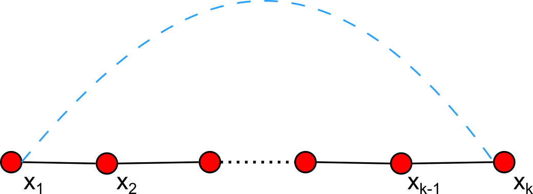
Figure 7: The scenario described in Lemma 25. The additional link is dashed in blue.

In fact, we can use the same reasoning to generalize for $c>1$. If two nodes are at a distance $L+1$ of each other, then there is a path with $L$ nodes connecting them. By establishing a link with cost $c$, we are shortening the distance between the end node to $\sim L/2$ nodes that lay on the other side of the line. The average reduction in distance is also $\approx L/2$, so by comparing $L^{2}\approx 4c$ we obtain a bound on $L$, as follows:

Lemma 27.

The longest distance between any node $i$ and node $j\in T_{B}$ is bounded by $2\sqrt{c_{B}}$. The longest distance between nodes $i,j\in T_{A}$ is bounded by $\sqrt{(1-2A)^{2}+4c_{A}}-2\left(A-1\right)$. In addition, if $c_{A}<A$ then there is a link between every two type-A nodes.

Proof.

We bound the maximal distance between two nodes by conisdering the cost reduction of establishing a direct link between the two nodes $i,j$ at the perimeter of a length $k$ line. We show that if the line length is $\geq\left\lfloor 2\sqrt{c_{B}}\right\rfloor$ then it is beneficial to establish such link. Assume $d(i,j)=k\geq\left\lfloor 2\sqrt{c_{B}}\right\rfloor>1$ and $i\in T_{B}$. Then there exist nodes $(x_{0}=i,x_{2},..x_{k-1}=j)$ such that $d(i,x_{\alpha})=\alpha$. By adding a link $(i,j)$ the change in cost of node $i$, $\Delta C(i,E+ij)$ is, according to lemma 25,

$$\Delta C(i,E+ij)$$

$$= c_{B}-\sum_{\alpha=1}^{k-1}d(i,x_{\alpha})(1+\delta_{x_{\alpha},A}(A-1))$$

$$+\sum_{\alpha=1}^{k-1}d^{\prime}(i,x_{\alpha})(1+\delta_{x_{\alpha},A}(A-1))$$

$$= c_{B}-\sum_{\alpha=1}^{k-1}\left(d(i,x_{\alpha})-d^{\prime}(i,x_{\alpha})\right)(1+\delta_{x_{\alpha},A}(A-1))$$

$$< c_{B}-\sum_{\alpha=1}^{k-1}d(i,x_{\alpha})+\sum_{\alpha=1}^{k-1}d^{\prime}(i,x_{\alpha})$$

$$< c_{B}-\frac{k\left(k-2\right)+mod(k,2)}{4}$$

$$< c_{B}-\frac{k\left(k-2\right)}{4}<0$$

where $d^{\prime}(i,x_{\alpha})<d(i,x_{\alpha})$ is the distance after the addition of the link $(i,j)$ and $\delta_{x_{\alpha},A}=1$ iff $x_{\alpha}\in T_{A}$. Therefore, it is of the interest of player $i$ to add the link.

Consider the case that $j\in T_{A}$ and

$$d(i,j)=k-1\geq\sqrt{(1-2A)^{2}+4c_{B}}-2\left(A-1\right)>1$$ (7)

The change in cost after the addition of the link $(i,j)$ is

$$c_{B}-\sum_{\alpha=1}^{k-1}d(i,x_{\alpha})(1+\delta_{x_{\alpha},A}(A-1))$$

$$+\sum_{\alpha=1}^{k-1}d^{\prime}(i,x_{\alpha})(1+\delta_{x_{\alpha},A}(A-1))$$

$$= c_{B}-\sum_{\alpha=1}^{k-1}\left(d(i,x_{\alpha})-d^{\prime}(i,x_{\alpha})\right)(1+\delta_{x_{\alpha},A}(A-1))$$

$$< c_{B}-\sum_{\alpha=1}^{k-2}d(i,x_{\alpha})+\sum_{\alpha=1}^{k-2}d^{\prime}(i,x_{\alpha})+A\left(d(i,x_{k})-d^{\prime}(i,x_{k})\right)$$

$$< c_{B}-\frac{k\left(k-2\right)+mod(k-1,2)}{4}-\left(k-1\right)A$$

$$+\left(k-1\right)+A-1$$

$$< c_{B}-\frac{k\left(k-2\right)}{4}-\left(A-1\right)\left(k-2\right)$$

$$= c_{B}-k^{2}/4-k(A-1)$$

$$< 0$$

Therefore it is beneficial for player $i$ to establish the link. Similarly, if $i\in T_{A}$ then eq. 7 is replaced by $k-1\geq\sqrt{(1-2A)^{2}+4c_{A}}-2\left(A-1\right)>1$.

In particular, if we do not omit the $mod(k-1,2)$ term and set $k=3$ we get that if $2\sqrt{(-1+A)A+c_{A}}-2(A-1)<2$ the distance between two type-A nodes is smaller than 2, in other words, they connected by a link. The latter expression can be recast to the simple form $c<A$.

Recall that if the cost of both parties is reduced (the change of cost of node $j$ is obtained by the change of summation to $0..k-1$) a link connecting them will be formed. Therefore, if $i,j\in T_{B}$ then maximal distance between then is $d(i,j)\leq max\{2\sqrt{c_{B}},1\}$ as otherwise it would be beneficial for both $i,j$ to establish a link that will reduce their mutual distance to $1.$ Likewise, if $i,j\in T_{A}$ then

$$d(i,j)\leq\sqrt{(1-2A)^{2}+4c_{A}}-2\left(A-1\right)$$

using an analogous reasoning. If $i\in T_{A}$ and $j\in T_{B}$ then it’ll be worthy for player $i$ to establish the link only if $d(i,j)\geq\left\lfloor 2\sqrt{c_{B}}\right\rfloor$. In this case it’ll be also worthy for player $j$ to establish the link since

$$d(i,j)\geq\left\lfloor 2\sqrt{c_{B}}\right\rfloor\geq\sqrt{(1-2A)^{2}+4c_{B}}-2\left(A-1\right)$$

and the link will be established. Notice however that if

$$\left\lfloor 2\sqrt{c_{B}}\right\rfloor\geq d(i,j)\geq\sqrt{(1-2A)^{2}+4c_{A}}-2\left(A-1\right)$$

then although it is worthy for player $j$ to establish the link, it is isn’t worthy for player $i$ to do so and the link won’t be established. This concludes our proof. ∎

Lemma 27 indicates that if $1<c_{A}<A$ then the type $A$ nodes will form a clique (the “nucleolus” of the network). The type $B$ nodes form structures that are connected to the type $A$ clique (the network nucleolus). These structures are not necessarily trees and will not necessarily connect to a single point of the type-A clique only. This is indeed a very realistic scenario, found in many configurations.

If $c_{A}>A$ then the type-A clique is no longer stable. This setting does not correspond to the observed nature of the inter-AS topology and we shall focus in all the following sections on the case $1<c_{A}<A$. Nevertheless, as a flavor of the results for $c_{A}>A$ we present the following proposition, which is stated for general heterogeneity of players, rather than a dichotomy of types. Here, we denote that the relative importance of player $j$ in player $i$’s concern is as $A_{ij}$.

Proposition 28.

Assume the cost function of player $i$ is given by the form

$$C(i)\triangleq deg(i)\cdot c+\sum_{j\in T_{A}}A_{ij}d(i,j)$$

where either $c>A_{ij}$ or $c>A_{ji}$. Then a star is a stable formation. Furthermore, if $A_{ij}=A_{j}$ define $j^{*}$ as the node for which $A_{j^{*}}$is maximal. Then a star with node $j^{*}$ at its center is the optimal stable structure in terms of social utility.

Proof.

Clearly, it is not worthy for player either player $i$ or player $j$ to reduce their distance from 2 to the 1 since either

$$\Delta C(i,E+ij)=c-A_{ij}>0$$

or

$$\Delta C(j,E+ij)=c-A_{ji}>0$$

and the link $(i,j)$ will not be established. It is also not possible to remove any links without disconnecting the network. This proofs the stability of the star.

Regarding the optimality of the network structure, a player must have be connected to at least one node in order to be connected to the network. With no additional links, the minimal distance to all other nodes is 2 and the discussion before indicates it is not beneficial to add extra links to reduce the distance to only one node. The social cost of a star with $x_{0}$ at its center is

$$\sum C(i) = c\left(N-1\right)+2(N-1)\sum_{x\neq x_{0}}A_{x}$$

$$+(N-1)A_{x_{0}}+\sum_{x\neq x_{0}}A_{x}$$

$$= c\left(N-1\right)+2(N-1)\sum_{x}A_{x}$$

$$-(N-1)A_{x_{0}}-\sum_{x\neq x_{0}}A_{x}$$

where $N$ is the number of players, $d(x,x^{\prime})=2$ for all $x,x^{\prime}\neq x_{0}$ and $d(x,x_{0})=1$. The first two terms are constants. In order to minimize the latter expression, one needs to maximize

$$(N-1)A_{x_{0}}+\sum_{x\neq x_{0}}A_{x}=(N-2)A_{x_{0}}+\sum_{x}A_{x}$$

the latter is clearly maximized by choosing $A_{x_{0}}$as maximal. Hence, the optimal star is a star with $x_{0}$at its center.

Assume the optimal stable structure is not a star. Then, there is at least three nodes $i,y_{1},y_{2}$ such that $d(i,y_{1})=d(i,y_{2})=d(y_{1},y_{2})=1$ as in the star configuration the link’s term is minimal and $d(x,x^{\prime})=2$ for all $x,x^{\prime}\neq x_{0}$ and $d(x,x_{0})=1$. However, the above discussion shows the annihilation of at least one of the links of the clique $(y_{1},y_{2},i$) is beneficial for at least one of the players and this structure would not be stable. ∎

B.1.3 Equilibria’s properties

Here we describe common properties of all pair-wise equilibria. We start by noting that, unlike the findings of several other studies Arcaute et al. [6, 7], Fabrikant et al. [14], Nisan N. [22], in our model, at equilibrium, the type-B nodes are not necessarily organized in trees. This is shown in the next example.

Figure 8: Non optimal networks. The type-A clique is in blue squares, the type-B players are in red circles. a) The network described in Example 29. b) A poor equilibrium, as described in the appendix.

Example 29.

Assume for simplicity that $c_{A}=c_{B}=c$. Consider a line of length $k$ of type B nodes, $(1,2,3...,k)$ such that $\sqrt{8c}>k+1>\sqrt{2c}$ or equivalently $\left(k+1\right)^{2}<8c<4\left(k+1\right)^{2}$ . In addition, the links $(j_{1},1)$ and $(j_{2},k)$ exist, where $j\in T_{A}$, i.e., the line is connected at both ends to different nodes of the type-A clique, as depicted in Fig 8. We show in the appendix that this is a stabilizable graph.

We now show that this structure is stabilizable. For simplicity, assume $mod(k-1,4)=0$ ($k$ is odd and $\frac{k-1}{2}$ is odd).

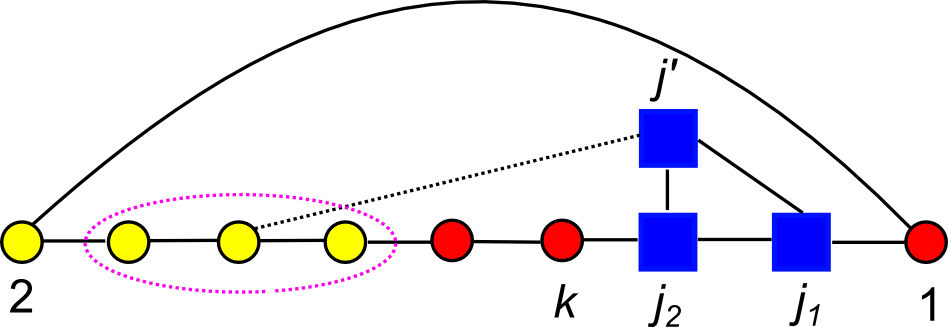
Figure 9: A line of $k=7$ nodes. By removing the link $(1,2)$ only the distances from player 1 to the yellow players are affected. By establishing the link $(j,4)$ only the distances from player $j^{\prime}$ to the players encircled by the purple dashed ellipse are affected.

Any link removal $(x_{1},x_{2})$ in the circle $(j_{1},1...k,j_{2},j_{1})$ will result in a line with nodes $x_{1}$ and $x_{2}$ at its ends (Fig. 9). The type-B players that have the most incentive to disconnect a link are either node $1$ or node $k$, as the type-A nodes will be closest to either one of them after the link removal (at distances one and two hops, Fig. 9). Therefore, if players $1$ or $k$ would not deviate, no type-B player will deviate as well.

W.l.o.g, we discuss node 1. Since $c_{B}<A$, it is not beneficial for it to disconnect the link $(j_{1},1)$. Assume the link $(1,2)$ is removed. A simple geometric observation shows that the distance to nodes $\{2,..,\frac{k+3}{2}\}$ is affected, while the distance to all the other nodes remains intact (Fig. 9). The mean increase in distance is $\frac{k+1}{2}$ and the number of affected nodes is $\frac{k+1}{2}$ . However,

$$\Delta C(1,E-12)=c-\frac{(k+1)}{2}^{2}<0$$

and player $1$ would prefer the link to remain. The same calculation shows that it is not beneficial for player $j_{1}$ to disconnect $(j_{1},1)$.

Clearly, if it not beneficial for $j\in T_{A},\,j\neq j_{1},j_{2}$ to establish an additional link to a type-B player then it is not beneficial to do so for $j_{1}$ or $j_{2}$ as well. The optimal additional link connecting $j$ and a type-B player is $\mathcal{E}=(j,\frac{k+1}{2})$, that is, a link to the middle of the ring (Fig. 9). A similar geometric observation shows that by establishing this link, only the distances to nodes $\left\{\frac{k-1}{4},...,\frac{3k+1}{4}\right\}$ are affected (Fig. 9). The reduction in cost is

$$\Delta C(j,E+\mathcal{E})=c-\frac{(k+1)}{8}^{2}>0$$

and it is not beneficial to establish the link.

In order to complete the proof, we need to show that no additional type-B to type-B links will be formed. By establishing such link, the distance of at least one of the parties to the type-A clique is unaffected. The previous calculation shows that by adding such link the maximal reduction of cost due to shortening the distance to type-B players is bounded from above by $\frac{(k+1)}{8}^{2}$. Therefore, as before, no additional type-B to type-B links will be formed.

This completes the proof that this structure is stabilizable.

Next, we bound from below the number of equilibria. For simplicity, we discuss the case where $c_{A}=c_{B}=c$. We accomplish that by considering the number of equilibria where the type-B players are organized in a forest (multiple trees) and the allowed forest topologies. The following lemma restricts the possible sets of trees in an equilibrium. Intuitively, this lemma states that we can not have two “heavy” trees, “heavy” meaning that there is a deep sub-tree with many nodes, as it would be beneficial to make a shortcut between the two sub-trees.

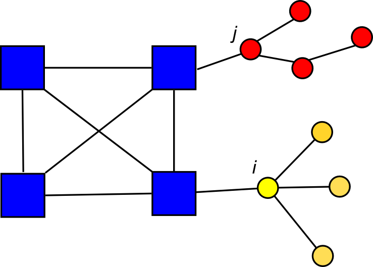
Figure 10: Node $j$ is on the third level of the tree of formed by starting a BFS from node $i$, as discussed in lemma 30. The forest of type-B nodes is composed of two trees, in yellow and red (lemma 31). Their roots are $i$ and $j,$ correspondingly. The maximal depth in this forest is three.

Lemma 30.

Assume $c_{A}=c_{B}=c$. Consider the BFS tree formed starting from node $i.$ Assume that node $j$ is $k$ levels deep in this tree. Denote the sub-tree of node $j$ in this tree by $\mathcal{T}_{i}(j)$ (Fig. 10) In a link stable equilibrium, the number of nodes in sub-trees satisfy either $|\mathcal{T}_{i}(j)|<c/k$ or $|\mathcal{T}_{j}(i)|<c/k$.

Proof.

Assume $|\mathcal{T}_{i}(j)|>c/k$. Consider the change in cost of player $i$ after the addition of the link $(i,j)$

$$\Delta C(i,E+ij)$$

$$= c+\sum_{x_{\alpha}\in\mathcal{T}i(j)}d^{\prime}(i,x_{\alpha})(1+\delta_{x_{\alpha},A}(A-1))$$

$$+\sum_{x_{\alpha}\notin\mathcal{T}_{i}(j)}d^{\prime}(i,x_{\alpha})(1+\delta_{x_{\alpha},A}(A-1))$$

$$-\sum_{x_{\alpha}\in\mathcal{T}_{i}(j)}d(i,x_{\alpha})(1+\delta_{x_{\alpha},A}(A-1))$$

$$-\sum_{x_{\alpha}\notin\mathcal{T}_{i}(j)}d(i,x_{\alpha})(1+\delta_{x_{\alpha},A}(A-1))$$

$$= c+\sum_{x_{\alpha}\in\mathcal{T}_{i}(j)}\left(d^{\prime}(i,x_{\alpha})-d(i,x_{\alpha})\right)(1+\delta_{x_{\alpha},A}(A-1))$$

$$+\sum_{x_{\alpha}\notin\mathcal{T}_{i}(j)}\left(d^{\prime}(i,x_{\alpha})-d(i,x_{\alpha})\right)(1+\delta_{x_{\alpha},A}(A-1))$$

$$< c+\sum_{x_{\alpha}\in\mathcal{T}_{i}(j)}\left(d^{\prime}(i,x_{\alpha})-d(i,x_{\alpha})\right)$$

$$= c-k|T_{i}(j,k)|$$

$$< 0$$

since the distance was shorten by $k$ for every node in the sub-tree of $j$.

Therefore, it is beneficial for player $i$ to establish the link. Likewise, if $|\mathcal{T}_{j}(i)|<c/k$ then it would be beneficial for player $j$ to establish the link and the link will be established. Hence, one of the conditions must be violated. ∎

The following lemma considers the structure of the type-B players’ sub-graph. It builds on the results of lemma 30 to reinforce the restrictions on trees, showing that trees must be shallow and small.

Lemma 31.

Assume $c_{A}=c_{B}=c$. If the sub-graph of type-B nodes is a forest (Fig. 10), then there is at most one tree with depth greater than $\sqrt{c/2}$ and there is at most one tree with more than $c/2$ nodes. The maximal depth of a tree in the forest is $\sqrt{2c}-1$. Every type-B forest in which every tree has a maximal depth of $\min\left\{\sqrt{c/2},\sqrt{c}-3\right\}$ and at most $\min\left\{c/2,\sqrt{c}\right\}$ nodes is stabilizable.

Proof.

Assume there are two trees $S_{1},S_{2}$ that have depth greater than $\sqrt{c/2}$ . The distance between the nodes at the lowest level is greater than $2\sqrt{c/2}+1$ as the trees are connected by at least one node in the type-A clique, $d(i,j)\geq 2$ (Fig. 10). This contradicts with Lemma 27.

Assume there are two trees $S_{1},S_{2}$ with roots $i,j$ that have more than $c/2$ nodes. In the BFS tree that is started from node $i$ node $j$ is at least in the second level (as they are connected by at least one node in the type-A clique). This contradicts with Lemma 30.

Finally, following the footsteps of Lemma 30 proof, consider two trees $\mathcal{T}_{i}$ and $\mathcal{T}_{j}$, with corresponding roots $i$ and $j$ (i.e., nodes $i$ and $j$ have a direct link with the type-A clique). Consider a link $(x,y)$, where $x\in\mathcal{T}_{i}$ and $y\in\mathcal{T}_{j}$. At least one of them does not reduce its distance to the type-A clique by establishing this link. W.l.o.g, we’ll assume this is true for player $x$. Therefore,

$$\Delta C(x,E+xy)$$

$$= c+\sum_{z\in\mathcal{T}_{j}}\left(d^{\prime}(z,x)-d(z,x)\right)$$

$$> 0$$

as the maximal reduction in distance is $\sqrt{c}$ and the maximal number of nodes in $\mathcal{T}_{j}$ is also $\sqrt{c}$. Therefore, it is not beneficial for player $x$ to establish this link, and the proof is completed. ∎

Finally, the next proposition provides a lower bound on the number of link-stable equilibria by a product of $|T_{A}|$ and a polynomial with a high degree ($\approx 2^{\sqrt{c}}$) in $|T_{B}|$.

Proposition 32.

Assume $c_{A}=c_{B}=c$. The number of link-stable equilibria in which the sub-graph of $T_{B}$ is a forest is at least $o(|T_{A}||T_{B}|^{N_{c}})$, where $N_{c}=o(2^{\frac{\sqrt{c}}{2}}/\sqrt{c})$ is a function of $c$ only. Therefore, the number of link-stable equilibria is at least $o(|T_{A}||T_{B}|^{N_{c}}).$

Proof.

For simplicity, we consider the case where $c\gg 1$ and count the number of different forests that are composed of trees up to depth $\sqrt{c/2}$ and exactly $\sqrt{c}$ nodes. Let’s define the number of different trees by $N_{c}$. Note that $N_{c}$ is independent of $|T_{B}|.$ The number of different forests of this type is bound from below by the expression $\left(\begin{array}[]{c}|T_{B}|+N_{c}\\ N_{c}\end{array}\right)$. Using Striling’s approximation $\left(\begin{array}[]{c}|T_{B}|+N_{c}\\ N_{c}\end{array}\right)=o(|T_{B}|^{N_{c}})$. The number $N_{C}$ can be bounded in a similar fashion by $\left(\begin{array}[]{c}\left\lfloor\sqrt{c}\right\rfloor\\ \left\lfloor\sqrt{c/2}\right\rfloor\end{array}\right)=o(2^{\frac{\sqrt{c}}{2}}/\sqrt{c})$, which is the number of trees with $\sqrt{c}$ elements, depth $\sqrt{c/2}$ and only one non-leaf node at each level of tree.

Each tree can be connected to either one of the type-A nodes, and therefore the number of possible configurations is at least $o(|T_{A}||T_{B}|^{N_{c}})$ . ∎

To sum up, while there are many equilibria, in all of them nodes cannot be too far apart, i.e., a small-world property. Furthermore, the trees formed are shallow and are not composed of many nodes.

B.1.4 Price of Anarchy & Price of Stability

As there are many possible link-stable equilibria, a discussion of the price of anarchy is in place. First, we explicitly find the optimal configuration. Although we establish a general expression for this configuration, it is worthy to also consider the limiting case of a large network, $|T_{B}|\gg 1,|T_{A}|\gg 1$. Moreover, typically, the number of major league players is much smaller than the other players, hence we also consider the limit $|T_{B}|\gg|T_{A}|\gg 1$.

Figure 11: The optimal solution, as described in Lemma 33. If $\left(A+1\right)/2<c$ the optimal solution is described by a), otherwise by b). When monetary transfers (section 5) are allowed, both configurations are stabilizable. Otherwise, only a) is stabilizable.

Proposition 33.

Consider the network where the type $B$ nodes are connected to a specific node $j\in T_{A}$ of the type-A clique. The social cost in this stabilizable network (Fig. 11(a)) is

$$\mathcal{S} = 2|T_{B}|\left(|T_{B}|-1+c+\left(A+1\right)(|T_{A}|-1/2)\right)+|T_{A}|\left(|T_{A}|-1\right)\left(c_{A}+A\right).$$

Furthermore, if $|T_{B}|\gg 1,|T_{A}|\gg 1$ then, omitting linear terms in $|T_{B}|,|T_{A}|$,

$$\mathcal{S}=2|T_{B}|(|T_{B}|+\left(A+1\right)|T_{A}|)+|T_{A}|^{2}\left(c+A\right).$$

Moreover, if $\frac{A+1}{2}\leq c$ then this network structure is socially optimal and the price of stability is $1$, otherwise the price of stability is

$$PoS=\frac{2|T_{B}|(|T_{B}|+\left(A+1\right)|T_{A}|)+|T_{A}|^{2}\left(c_{A}+A\right)}{2|T_{B}|\left(|T_{B}|+\left(\frac{A+1}{2}+c\right)|T_{A}|\right)+|T_{A}|^{2}\left(c_{A}+A\right)}.$$

Finally, if $|T_{B}|\gg|T_{A}|\gg 1$, then the price of stability is asymptotically $1$.

Proof.

This structure is immune to removal of links as a disconnection of a $(type-B,type-A)$ link will disconnect the type-B node, and the type-A clique is stable (lemma 27). For every player $j$ and $i\in T_{B}$, any additional link $(i,j)$ will result in $\Delta C(j,E+ij)\geq c_{B}-1>0$ since the link only reduces the distance $d(i,j)$ from 2 to 1. Hence, player $j$ has no incentive to accept this link and no additional links will be formed. This concludes the stability proof.

We now turn to discuss the optimality of this network structure. First, consider a set of type-A players. Every link reduce the distance of at least two nodes by at least one, hence the social cost change by introducing a link is negative, since $2c_{A}-2A<0$. Therefore, in any optimal configuration the type-A nodes form a complete graph. The other terms in the social cost are due to the inter-connectivity of type-B nodes and the type-A to type-B connections. As $deg(i)=1$ for all $i\in T_{B}$ the cost due to link’s prices is minimal. Furthermore, $d(i,j)=1$ and the distance cost to node $j$ (of type A) is minimal as well. For all other nodes $j^{\prime}$, $d(i,j^{\prime})=2$.

Assume this configuration is not optimal. Then there is a topologically different configuration in which there exists an additional node $j^{\prime}\in T_{A}$ for which $d(i,j^{\prime})=1$ for some $i\in T_{B}$. Hence, there’s an additional link $(i,j)$. The social cost change is $2c+2+\delta_{x_{\alpha},A}(A-1)$ . Therefore, if $\frac{A+1}{2}\leq c$ this link reduces the social cost. On the other hand, if $\frac{A+1}{2}>c$ every link connecting a type-B player to a type-A player improves the social cost, although the previous discussion show these link are unstable. In this case, the optimal configuration is where all type-B nodes are connected to all the type-A players, but there are no links linking type-B players. This concludes the optimality proof.

The cost due to inter-connectivity of type A nodes is

$$c_{A}|T_{A}|\left(|T_{A}|-1\right)+A|T_{A}|\left(|T_{A}|-1\right)=|T_{A}|\left(|T_{A}|-1\right)\left(c_{A}+A\right).$$

The first expression is due to the cost of $|T_{A}|$ clique’s links and the second is due to distance (=1) between each type-A node. The distance of each type B nodes to all the other nodes is exactly 2, except to node $j$, to which its distance is 1. Therefore the social cost due to type B nodes is

$$2|T_{B}|(|T_{B}|-1)+2c_{B}|T_{B}|+2\left(A+1\right)|T_{B}|\left(\left(|T_{A}|-1\right)+\left(A+1\right)+2\left(A+1\right)(|T_{A}|-1)\right)$$

$$= 2|T_{B}|\left(|T_{B}|-1+c_{B}+\left(A+1\right)(|T_{A}|-1/2)\right).$$

The terms on the left hand side are due to (from left to right) the distance between nodes of type B, the cost of each type-B’s single link, the cost of type-B nodes due to the distance (=2) to all member of the type-A clique bar $j$ and the cost of type $B$ nodes due to the distance (=1) to node $j$. The social cost is

$$\sum C(i) = 2|T_{B}|\left(|T_{B}|-1+c+\left(A+1\right)(|T_{A}|-1/2)\right)+|T_{A}|\left(|T_{A}|-1\right)\left(c_{A}+A\right).$$

To complete the proof, note that if $\frac{A+1}{2}>c$ the latter term in the social cost of the optimal (and unstable) solution is

$$2|T_{B}|(|T_{B}|-1)+2c|T_{B}|\left(1+|T_{A}|\right)+\left(A+1\right)|T_{B}||T_{A}|=2|T_{B}|\left(|T_{B}|-1+\left(\frac{A+1}{2}+c\right)|T_{A}|\right).$$

As the number of links is $|T_{B}|\left(1+|T_{A}|\right)$ and the distance of type-B to type-A nodes is 1. The optimal social case is then

$$2|T_{B}|\left(|T_{B}|-1+\left(\frac{A+1}{2}+c\right)|T_{A}|\right)+|T_{A}|\left(|T_{A}|-1\right)\left(c_{A}+A\right).$$

Considering all quantities in the limit $|T_{B}|\gg 1,|T_{A}|\gg 1$ completes the proof.∎

Next, we evaluate the price of anarchy. The social cost in the stabilizable topology presented in Fig 8, composed of a type-A clique and long lines of type-B players, is calculated in the appendix. The ratio between this value and the optimal social cost constitutes a lower bound on the price of anarchy. An upper bound is obtained by examining the social cost in any topology that satisfies Lemma 27. The result in the large network limit is presented by the following proposition.

Next, we evaluate the price of anarchy. In order to do that, we use the following two lemmas. The first lemma evaluates a lower bound by considering the social cost in the stabilizable topology presented in Fig 8(b), composed of a type-A clique and long lines of type-B players. Later on, an upper bound is obtained by examining the social cost in any topology that satisfies Lemma 27.

For simplicity, in the following lemma we assume that $|T_{B}|=\min\left\{\left\lfloor\sqrt{4c_{A}}\right\rfloor,\left\lfloor\sqrt{4c_{B}/5}\right\rfloor\right\}m$ where $m\in\mathcal{N}$

Lemma 34.

Consider the network where the type B nodes are composed of $m$ long lines of length $k=\min\left\{\left\lfloor\sqrt{3c_{A}}\right\rfloor,\left\lfloor\sqrt{4c_{B}/5}\right\rfloor\right\}$, and all the lines are connected at $j\in T_{A}$. The total cost in this stabilizable network is

$$S = |T_{A}|\left(|T_{A}|-1\right)\left(c_{A}/2+A\right)+2c_{B}|T_{B}|+\left(A+1\right)|T_{B}|\left(|T_{A}|-1\right)\left(k+3\right)/2$$

$$+|T_{B}|\left(\left(A+1\right)\left(k+1\right)/2+2k-4\right)+2|T_{B}|^{2}(k+2)^{2}-2m$$

if $|T_{B}|\gg 1,|T_{A}|\gg 1$ then

$$S = \left(A+1\right)|T_{A}|\left|T_{B}\right|o(c)$$

$$+|T_{A}|^{2}\left(c+A\right)+\left|T_{B}\right|^{2}o(c)$$

Proof.

For simplicity, we assume $c_{B}\leq 20c_{A}$. First, for the same reason as in Prop. 33, this network structure is immune to removal of links. Consider $j^{\prime}\in T_{A},j^{\prime}\neq j$. Let us observe the chain $(j,1,2,3,...k)$ where $1,2,3...k\in T_{B}$.

By establishing a link to some node $k\geq x\geq 1$, the change in cost of player $j^{\prime}$ is

$$\Delta C(j^{\prime},E+j^{\prime}k)=c_{A}-\sum_{i=1}^{k}\left(d(i,j^{\prime})-d^{\prime}(i,j^{\prime})\right).$$

Note that this distance is non-zero only for a node $i$ that satisify

$$i>(x-i)+1$$

or $i<\left(x+1\right)/2$. The maximal reduction in distance is bounded by noting that the optimal link is to node $x$ such that $2k/3+1\geq x\geq 2k/3-1$. Hence,

$$\sum_{i=\left\lceil\left(x+1\right)/2\right\rceil}^{k}\left(d(i,j^{\prime})-d^{\prime}(i,j^{\prime})\right) \leq \frac{\left(\left\lceil\left(x+1\right)/2\right\rceil+2+k\right)\left(k-\left\lceil\left(x+1\right)/2\right\rceil\right)}{2}-2\sum_{i=1}^{k-x-1}i$$

$$\leq \frac{\left(x/2+1+k\right)\left(k-x/2\right)}{2}-(k-x)\left(k-x-2\right)$$

$$\leq \frac{\left(4k/3+1\right)\left(2k/3+1\right)}{2}-(k-2k/3-1)\left(k-2k/3-3\right)$$

$$\leq 4k^{2}/9+4k/3+1-(k/3-1)\left(k/3-3\right)$$

$$\leq 4k^{2}/9+4k/3+1-k^{2}/9-4k/3-4$$

$$\leq k^{2}/3-3$$

and we have,

$$\Delta C(j^{\prime},E+j^{\prime}k) = c_{A}-k^{2}/3+3$$

$$> c_{A}-\frac{k^{2}}{3}>0$$

by lemma 25 and noting the distance to player $j$ is unaffected. Therefore there is no incentive for player $j^{\prime}$ to add the link $(j^{\prime},k)$. The same calculation indicates that no additional link $(i,i^{\prime})$ will be formed between two nodes on the same line.

Consider two lines of length $k$, $(j,x_{1},x_{2},...x_{k})$ and $(j,y_{1},y_{2},...y_{k})$. Consider the addition of the link $(x_{k},y_{\left\lfloor k+1/2\right\rfloor})$. That is, the addition of a link from an end of one line to the middle player on another line. This link is optimal in $x_{k}^{\prime}$s concern, as it minimizes the sum of distances from it to players on the other line. The change in cost is (see appendix)

$$\Delta C(x_{k},E+x_{k}y_{\left\lfloor k+1/2\right\rfloor})=c_{B}-5k^{2}/4>0.$$

Note that

$$\Delta C(x_{k},E+x_{k}y_{\left\lfloor k+1/2\right\rfloor}) \leq \Delta C(x_{k},E+x_{k}y_{i})$$

for any other $i=1..k$, since a player gains the most from establishing a link to the another line is the player that is furthest the most from that line, i.e., the player at the end of the line. This concludes the stability proof.

The total cost due to type-B nodes is

$$2c_{B}|T_{B}|+\left(A+1\right)|T_{B}|\left(|T_{A}|-1\right)\left(k+3\right)/2$$

$$+|T_{B}|\left(A+1\right)\left(k+1\right)/2+2m(k-1)^{2}+2(m-1)mk^{2}(k+2)^{2}.$$

The terms represent (from left to right) the links’ cost, the cost due to the type-B players’ distances to the type-A clique’s nodes (except $j$), the cost due to the type-B players’ distances from node $j$, the cost due to intra-line distances and the cost due inter-lines distances. By using the relation $|T_{B}|=km$ we have

$$=2 c_{B}|T_{B}|+\left(A+1\right)|T_{B}|\left(|T_{A}|-1\right)\left(k+3\right)/2$$

$$+|T_{B}|\left(A+1\right)\left(k+1\right)/2+2\left(|T_{B}|-m\right)(k-1)+2|T_{B}|^{2}(k+2)^{2}-2|T_{B}|m(k+2)$$

$$= 2c_{B}|T_{B}|+\left(A+1\right)|T_{B}|\left(|T_{A}|-1\right)\left(k+3\right)/2$$

$$+|T_{B}|\left(\left(A+1\right)\left(k+1\right)/2+2k-4\right)+2|T_{B}|^{2}(k+2)^{2}-2m.$$

The total cost due to type-A is as before

$$|T_{A}|\left(|T_{A}|-1\right)\left(c_{A}+A\right).$$

Therefore,

$$\sum C(i) = |T_{A}|\left(|T_{A}|-1\right)\left(c_{A}/2+A\right)+2c_{B}|T_{B}|+\left(A+1\right)|T_{B}|\left(|T_{A}|-1\right)\left(k+3\right)/2$$

$$+|T_{B}|\left(\left(A+1\right)\left(k+1\right)/2+2k-4\right)+2|T_{B}|^{2}(k+2)^{2}-2m$$

$$\rightarrow |T_{A}|^{2}\left(c_{A}+A\right)+\left(A+1\right)|T_{A}|\left|T_{B}\right|o(k)+\left|T_{B}\right|^{2}o(k).$$

∎

The most prevalent situation is when $|T_{B}|\gg|T_{A}|\gg 1$. In this case we can bound the price of anarchy to be at least $o(k^{2})=o(c_{B})$.

The next lemma bounds the price of anarchy from above by bounding the maximal total cost in the a link-stable equilibrium.

Lemma 35.

The worst social utility in a link stable equilibrium is at most

$$|T_{A}|^{2}\left(c_{A}+A\right)+|T_{B}|^{2}\left(c_{B}+\left\lfloor 2\sqrt{c_{B}}\right\rfloor\right)$$

$$+ \left(A+1\right)\left\lfloor 2\sqrt{c}\right\rfloor|T_{A}||T_{B}|$$

Proof.

The total cost due to the inter-connectivity of the type-A clique is identical for all link stable equilibria and is $|T_{A}|\left(|T_{A}|-1\right)\left(c_{A}+A\right)$. The maximal distance between nodes $i,j$ according to Lemma 27 is $\left\lfloor 2\sqrt{c_{B}}\right\rfloor$ and therefore the maximal cost due to the distances between type-B nodes is $\left\lfloor 2\sqrt{c_{B}}\right\rfloor|T_{B}|\left(|T_{B}|-1\right)$. Likewise, the maximal cost due to the distance between type-B nodes and the type-A clique is $\left(A+1\right)\left\lfloor 2\sqrt{c}\right\rfloor|T_{A}||T_{B}|$. Finally, the maximal number of links between type-B nodes is $|T_{B}|\left(|T_{B}|-1\right)/2$ and the total cost due to this part is $|T_{B}|\left(|T_{B}|-1\right)c_{B}$.

Adding all the terms we obtain the required result. ∎

To summarize, we state the previous results in a proposition.

Proposition 36.

If $c_{B}<A$ and $|T_{B}|\gg|T_{A}|\gg 1$ the price of anarchy is $\Theta(c_{B})$.

B.2 Basic model - Dynamics

The Internet is a rapidly evolving network. In fact, it may very well be that it would never reach an equilibrium as ASs emerge, merge, and draft new contracts among them. Therefore, a dynamic analysis is a necessity. We first define the dynamic rules. Then, we analyze the basin of attractions of different states, indicating which final configurations are possible and what their likelihood is. We shall establish that reasonable dynamics converge to just a few equilibria. Lastly, we investigate the speed of convergence, and show that convergence time is linear in the number of players.

B.2.1 Setup & Definitions

At each point in time, the network is composed of a subset $N^{\prime}\subset T_{A}\cup T_{B}$ of players that already joined the game. The cost function is calculated with respect to the set of players that are present (including those that are joining) at the considered time. The game takes place at specific times, or turns, where at each turn only a single player is allowed to remove or initiate the formation of links. We split each turn into acts, at each of which a player either forms or removes a single link. A player’s turn is over when it has no incentive to perform additional acts.

Definition 37.

Dynamic Rule #1: In player $i$’s turn it may choose to act $m\in\mathcal{N}$ times. In each act, it may remove a link $(i,j)\in E$ or, if player $j$ agrees, it may establish the link $(i,j)$. Player $j$ would agree to establish $(i,j)$ iff $C(j;E+(i,j))-C(j;E)<0$.

The last part of the definition states that, during player’s $i$ turn, all the other players will act in a greedy, rather than strategic, manner. For example, although it may be that player $j$ prefers that a link $(i,j^{\prime})$ would be established for some $j^{\prime}\neq j$, if we adopt Dynamic Rule #1 it will accept the establishment of the less favorable link $(i,j).$ In other words, in a player’s turn, it has the advantage of initiation and the other players react to its offers. This is a reasonable setting when players cannot fully predict other players’ moves and offers, due to incomplete information [7] such as the unknown cost structure of other players. Another scenario that complies with this setting is when the system evolves rapidly and players cannot estimate the condition and actions of other players.

The next two rules consider the ratio of the time scale between performing the strategic plan and evaluation of costs. For example, can a player remove some links, disconnect itself from the graph, and then pose a credible threat? Or must it stay connected? Does renegotiating take place on the same time scale as the cost evaluation or on a much shorter one? The following rules address the two limits.

Definition 38.

Dynamic Rule #2a: Let the set of links at the current act $m$ be denoted as $E_{m}$. A link $(i,j)$ will be added if $i$ asks to form this link and $C(j;E_{m}+ij)<C(j;E_{m})$. In addition, any link $(i,j)$ can be removed in act $m.$

The alternative is as follows.

Definition 39.

Dynamic Rule #2b: In addition to Dynamic Rule #2a, player $i$ would only remove a link $(i,j)$ if $C(i;E_{m}-ij)>C(i;E_{m})$ and would establish a link if both $C(j;E_{m}+ij)<C(j;E_{m})$ and $C(i;E_{m}+ij)<C(i;E_{m})$.

The difference between the last two dynamic rules is that, according to Dynamic Rule #2a, a player may perform a strategic plan in which the first few steps will increase its cost, as long as when the plan is completed its cost will be reduced. On the other hand, according to Dynamic Rule #2b, its cost must be reduced at each act, hence such “grand plan” is not possible. Note that we do not need to discuss explicitly disconnections of several links, as these can be done unilaterally and hence iteratively.Finally, the following lemma will be useful in the next section.

Lemma 40.

Assume $N$ players act consecutively in a (uniformly) random order at integer times, which we’ll denote by $t$. the probability $P(t)$ that a specific player did not act $k\mathcal{\in N}$ times by $t\gg N$ decays exponentially.

W.l.o.g, we’ll discuss player 1. Set $p=1/N.$ The probability that a player did not act $k$ times is given by the CDF Poisson distribution $f(t,p)$ as

$$P(t)=e^{-t/N}\sum_{i=0}^{k}\frac{1}{i!}\left(\frac{t}{N}\right)^{i}$$

and taking the limit $t\gg N$ concludes the proof.

B.2.2 Results

After mapping the possible dynamics, we are at a position to consider the different equilibria’s basins of attraction. Specifically, we shall establish that, in most settings, the system converges to the optimal network, and if not, then the network’s social cost is asymptotically equal to the optimal social cost. The main reason behind this result is the observation that a disconnected player has an immense bargaining power, and may force its optimal choice. As the highest connected node is usually the optimal communication partner for other nodes, new arrivals may force links between them and this node, forming a star-like structure. There may be few star centers in the graphs, but as one emerges from the other, the distance between them is small, yielding an optimal (or almost optimal) cost.

We outline the main ideas of the proof. The first few type-B players, in the absence of a type-A player, will form a star. The star center can be considered as a new type of player, with an intermediate importance, as presented in Fig. 12. We monitor the network state at any turn and show that the minor players are organized in two stars, one centered about a minor player and one centered about a major player (Fig. 12(a)). Some cross links may be present (Fig. 12). By increasing its client base, the incentive of a major player to establish a direct link with the star center is increased. This, in turn, increases the attractiveness of the star’s center in the eyes of minor players, creating a positive feedback loop. Additional links connecting it to all the major league players will be established, ending up with the star’s center transformation into a member of the type-A clique. On the other hand, if the star center is not attractive enough, then minor players may disconnect from it and establish direct links with the type-A clique, thus reducing its importance and establishing a negative feedback loop. The star will become empty, and the star’s center $x$ will be become a stub of a major player, like every other type-B player. The latter is the optimal configuration, according to proposition 9. We analyze the optimal choice of the active player, and establish that the optimal action of a minor player depends on the number of players in each structure and on the number of links between the major players and the minor players’ star center $x$. The latter figure depends, in turn, on the number of players in the star. We map this to a two dimensional dynamical system and inspect its stable points and basins of attraction of the aforementioned configurations.

Theorem 41.

If the game obeys Dynamic Rules #1 and #2a, then, in any playing order:

a) The system converges to a solution in which the total cost is at most

$$\mathcal{S} = |T_{A}|^{2}\left(c_{A}+A\right)-|T_{A}|\left(2A+c_{A}/2\right)+2|T_{B}|^{2}+|T_{B}|\left(A+2c_{B}\right)+3|T_{A}||T_{B}|\left(A+1\right)+2;$$

furthermore, by taking the large network limit $|T_{B}|\gg|T_{A}|\gg 1$, we have $\mathcal{S}/\mathcal{S}_{optimal}\rightarrow 1$ .

b) Convergence to the optimal stable solution occurs if either:

1) $A\cdot k_{A}>k+1$, where $k\geq 0$ is the number of type-B nodes that first join the network, followed later by $k_{A}$ consecutive type-A nodes (“initial condition”).

2)$A\cdot|T_{A}|>|T_{B}|$ (“final condition”).

c) In all of the above, if every player plays at least once in O(N) turns, convergence occurs after o(N) steps. Otherwise, if players play in a uniformly random order, the probability the system has not converged by turn $t$ decays exponentially with $t$.

Proof.

Assume $c_{A}\geq 2$. Denote the first type-A player that establish a link with a type-B player as $k$. First, we show that the network structure is composed of a type-A (possibly empty) clique, a set of type-B players $S$ linked to player $x$, and an additional (possibly empty) set of type-B players $L$ connected to the type-A player $k$. See Fig. 12(a) for an illustration. In addition, there is a set $D$ type-A nodes that are connected to node $x$, the star center. After we establish this, we show that the system can be mapped to a two dimensional dynamical system. Then, we evaluate the social cost at each equilibria, and calculate the convergence rate. We first assume $(k,x)\in E$ and discuss the case $(k,x)\notin E$ later.

.

Figure 12: a) The network structures described in Theorem 15. The type-A clique contains $|T_{A}|=4$ nodes (squares), and there are $|S|=5$ nodes in the star (red circles). There are $|L|=2$ nodes that are connected directly to node $k$ (yellow circles). The number of type-A nodes that are connected to node 1, the star center, is $|D|=2$ (green squares). b) The phase state of Theorem 15. The dotted green nullcline seperates the region in which $|S|$ increase or decrease. Similiary, the dotted red line is the nullcline for the regions in which $|D|$ increase or decrease. When monetary transfers are forbidden allowed this nullcline is shifted, and is presented by the dashed red line. (Proposition 24).

We prove by induction. At turn $t=2$, after the first two players joined the network, this is certainly true. Denote the active player at time $t$ as $r.$ Consider the following cases:

1. $r\in T_{A}$: Since $1<c_{A}<A,$ all links to the other type-A nodes will be established (lemma 9) or maintained, if $r$ is already connected to the network. Clearly, the optimal link in $r$’s concern is the link with star center $x$. As $c_{B}<A$ every minor player will accept a link with a major player even if it reduces its distance only by one. Therefore, the link $(r,x)$ is formed if the change of cost of the major player $r$,

$$\Delta C(r,E+rx)=c_{A}-|S|-1$$ (8)

is negative. In this case, the number of type A players connected to the star’s center, $|D|$, will increase by one. If this expression is positive and player $r$ is connected to at least another major player (as otherwise the graph is disconnected), the link will be dissolved and $|D|$ will be reduced by one. It is not beneficial for $r$ to form an additional link to any type-B player, as they only reduce the distance from a single node by one (see the discussion in lemma 9 in the appendix).

2. $r\in T_{B},\,r\neq x$ : First, assume that $r$ is a newly arrived player, and hence it is disconnected. Obviously, in its concern, a link to the star’s center, player $x$, is preferred over a link to any other type-B player. Similarly, a link to a type-A player that is linked with the star’s center is preferred over a link with a player that maintains no such link.

We claim that either $(r,k)$ or $(r,x)$ exists. Denote the number of type-A player at turn $t$ as $m_{A}.$ The link $(r,x)$ is preferred in $r$’s concern if the expression

$$C(r,E+rk)-C(r,E+rx)=-A(1+m_{A}-|D|)+1+|S|-|L|$$ (9)

is positive, and will be established as otherwise the network is disconnected. If the latter expression is negative, $(r,k)$ will be formed. The same reasoning as in case 1 shows that no additional links to a type-B player will be formed. Otherwise, if $r$ is already connected to the graph, than according to Dynamic Rule #2a, $r$ may disconnect itself, and apply its optimal policy, increasing or decreasing $|L|$ and $|S|$.

3. $r=x$, the star’s center: $r$ may not remove any edge connected to a type-B player and render the graph disconnected. On the other hand, it has no interest in removing links to major players. On the contrary, it will try to establish links with the major players, and these will be formed if eq. 8 is negative. An additional link to a minor player connected to $k$ will only reduce the distance to it by one and since $c_{B}>2$ player $x$ would not consider this move worthy.

The dynamical parameters that govern the system dynamics are the number of players in the different sets, $|S|$, $|L|$, and $|D|$. Consider the state of the system after all the players have player once. Using the relations $|S|+|L|+1=|T_{B}|,\>m_{A}=|T_{A}|$ we note the change in $|S|$ depends on $|S|$ and $|L|$ while the change in $|D|$ depends only on $|S|.$ We can map this to a 2D dynamical, discrete system with the aforementioned mapping. In Fig. 12 the state is mapped to a point in phase space $(|S|,|L|)$. The possible states lie on a grid, and during the game the state move by an single unit either along the $x$ or $y$ axis. There are only two stable points, corresponding to $|S|=0,|D|=0$, which is the optimal solution (Fig. 2(a)), and the state $|S|=|T_{B}|-1$ and $|D|=|T_{B}|$.

If at a certain time expression 8 is positive and expression 9 is negative (region 3 in Fig. 12(b)), the type-B players will prefer to connect to player $x$. This, in turn, increases the benefit a major player gains by establishing a link with player $x.$ The greater the set of type-A that have a direct connection with $x$, having $|D|$ members, the more utility a direct link with $x$ carries to a minor player. Hence, a positive feedback loop is established. The end result is that all the players will form a link with $x$. In particular, the type-A clique is extended to include the type-B player $x$. Likewise, if the reverse condition applies, a feedback loop will disconnect all links between node $x$ to the clique (except node $k$) and all type-B players will prefer to establish a direct link with the clique. The end result in this case is the optimal stable state. The region that is relevant to the latter domain is region 1.

However, there is an intermediate range of states, described by region 2 and region 4, in which the player order may dictate to which one of the previous states the system will converge. For example, starting from a point in region 4, if the type-A players move first, changing the $|D|$ value, than the dynamics will lead to region 1, which converge to the optimal solution. However, if the type-B players move first, then the system will converge to the other equilibrium point.

We now turn to calculate the social cost at the different equilibria. If $|D|=|T_{A}|$ and $|S|=|T^{\prime}_{B}|-1$, The network topology is composed of a $|T_{A}|$ members clique, all connected to the center $x$, that, in turn, has $|T_{B}|-1$ stubs. The total cost in this configuration is

$$S = |T_{A}|\left(|T_{A}|-1\right)\left(c_{A}+A\right)+2c_{B}|T_{B}|+\left(A+1\right)|T_{A}|+2\left(|T_{B}|-1\right)$$ (10)

$$+2\left(|T_{B}|-1\right)\left(A+1\right)+2\left(|T_{B}|-2\right)\left(|T_{B}|-1\right)+\left(c_{B}+c_{A}\right)|T_{A}|/2$$

where the costs are, from the left to right: the cost of the type-A clique, the cost of the type-B star’s links, the distance cost $(=1)$ between the clique and node $x$, the distance $(=1)$ cost between the star’s members and node $x$, the distance $(=2)$ cost between the clique and the star’s member, the distance $(=2)$ cost between the star’s members, and the cost due to major player link’s to the start center $x$. Adding all up, we have for the total cost

$$\mathcal{S} \leq |T_{A}|\left(|T_{A}|-1\right)\left(c+A\right)+2c_{B}|T_{B}|+\left(A+1\right)\left(3|T_{A}||T_{B}|+|T_{B}|\right)+2\left(|T_{B}|-1\right)^{2}.$$ (11)

Convergence is fast, and as soon as all players have acted three times the system will reach equilibrium. If every player plays at least once in $o(N$) turns convergence occurs after $o(N)$ turns, otherwise the probability the system did not reach equilibrium by time $t$ decays exponentially with $t$ according to lemma 14 (in the appendix).

We now relax our previous assumption $c_{A}\geq 2$. If $c_{A}\leq 2$ and the active player $r\in T_{A}$ then it will form a link with the star’s center according to eq. 8. If $r\in S$ it may establish a link $(r,j)$ with a type A player, which will later be replaced, in $j$’s turn, with the link $(j,x)$ according to the previous discussion. In the appendix we discuss explicitly the case where $(k,x)\notin E$ and show that in this case, additional links may be formed, e.g., a link between one of $k^{\prime}$s stubs, $i\in L$, and the star’s center $x$, as presented in Fig. 13. These links only reduce the social cost, and do not change the dynamics, and the system will converge to either one of the aforementioned states. Taking the limit $T_{B}\rightarrow\infty$ and $T_{B}\in\omega\left(T_{A}\right)$ in eq. 11, we get that $\mathcal{S}/\mathcal{S}_{optimal}\rightarrow 1$, and this concludes the proof.

Figure 13: Additional feasible cross-tiers links, as described in the appendix. The star players $S$ are in red, the set $L$ is in yellow. a) a link between the star center and $i\in L$. b) a cross-tier link $(i,j)$ where $i\in S,j\in L$. c) a minor player - major player link, $(i,j)$ where $i\in T_{A}$ and $j\in S.$

We now discuss explicitly the case where, at some point, the link $(k,x)$ is removed and assume that $c_{A}>2$, $c_{B}\geq 3$. In this case, the nullcline described by eq. 9 is replaced by

$$C(r,E+rk)-C(r,E+rx)=-A(1+m_{A}-|D|)+2\left(1+|S|-|L|\right).$$ (12)

This changes the regions according to Fig. 14. Region 1, which is the basin of attraction for the optimal configuration, increases its area, on the expense of region 4. The dynamical discussion as described for the case $(k,x)\in E$ is still applicable, and if the player play in a specific order, than the state vector $(|S|,|D|)$ will be in either region 1 or region 3 after $\Theta(1)$ turns. If the players play in random order, then the system might not converge only if player $k$ will play in every $\Theta(1)$ turns. This probability decays exponentially, according to lemma 40.

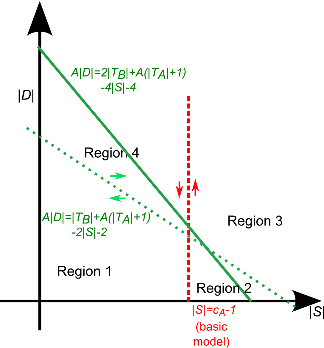
Figure 14: The dynamical regions with or without the link $(k,x)$. The dashed green represents the new type-B player preference nullcline when $(k,x)\in E$, according to eq. 9. According to eq. 12, the nullcline when $(k,x)\notin E$ is the solid green line.

In order to complete the proof, we now address the case $c_{A}\leq 2$. If $r\in S$, then $r$ will establish a link with $k\in T_{A}$, as the distance $d(r,k)$ is reduced by two. In this case, $r$ is a member of both $S$ and $L$, and we address this by the transformation $|S|\leftarrow|S|$, $|L|\leftarrow|L|+1$ and $|T_{B}|\leftarrow|T_{B}|+1.$ Similarly, if $r\in L$ then it will establish links with the star center $x$ if and only if $c_{B}\leq 2$. The analogous transformation is, $|S|\leftarrow|S|+1$, $|L|\leftarrow|L|$ and $|T_{B}|\leftarrow|T_{B}|+1.$ If $r\in T_{A}$ then it will act according to eq. 8. Finally, if $r=x$ than it may both establish link with players in $L$ and with major players according to the aforementioned discussion.

If $2\leq c_{A}\leq c_{B}$ than a link between player $k$ leaves, $i\in L$ and a star’s leaf, $j\in S$ is feasible and will be formed when either parties are selected as the active player. Every player $i$ may participate in only a single link of this type, as after its establishment the maximal distance between player $i$ to every other player is three, and an additioanl link will result in a reduction of the sum of distances by at most two. As before, additional links between the star center’s and the major players may be formed according to eq. 8.

Consider a link $(i,j)$ between $i\in L$ and a star’s leaf, $j\in S$. Neither $x$ nor $k$ has an incentive to disconnet either $(x,j)$ or $(k,s)$ as the distance is increased by at least three. Similarly, all the aforementioned links $(i,j)$ will not create an incentive for a link removal $(i,j^{\prime})$ or $(j,j^{\prime})$ by any former partner $j^{\prime}$ of the involved partied $i,j$.∎

If the star’s center has a principal role in the network, then links connecting it to all the major league players will be established, ending up with the star’s center transformation into a member of the type-A clique. This dynamic process shows how an effectively new major player emerges out of former type-B members in a natural way. Interestingly, Theorem 41 also shows that there exists a transient state with a better social cost than the final state. In fact, in a certain scenario, the transient state is better than the optimal stable state.

So far we have discussed the possibility that a player may perform a strategic plan, implemented by Dynamic Rule #2a. However, if we follow Dynamic Rule #2b instead, then a player may not disconnect itself from the graph. The previous results indicate that it is not worthy to add additional links to the forest of type-B nodes. Therefore, no links will be added except for the initial ones, or, in other words, renegotiation will always fail. The dynamics will halt as soon as each player has acted once. Formally:

Proposition 42.

If the game obeys Dynamic Rules #1 and #2b, then the system will converge to a solution in which the total cost is at most

$$\mathcal{S} = |T_{A}|\left(|T_{A}|-1\right)\left(c+A\right)+2\left(|T_{B}|-1\right)^{2}+\left(A+1\right)\left(3|T_{A}||T_{B}|-|T_{A}|+|T_{B}|\right)+2c|T_{B}|\,.$$

Furthermore, for $|T_{B}|\gg|T_{A}|\gg 1$, we have $\mathcal{S}/\mathcal{S}_{optimal}\leq 3/2.$ Moreover, if every player plays at least once in O(N) turns, convergence occurs after o(N) steps. Otherwise, e.g., if players play in a random order, convergence occurs exponentially fast.

Proof.

We discuss the case $c_{A}\geq 2$ and $c_{B}\geq 3$. The extension for $1>c_{B}>3$ appears in the appendix. The first part of the proof follows the same lines of the previous theorem (Theorem 41). We claim that at any given turn, the network structure is composed of the same structures as before. Here, we discuss the scenario where $(k,x)\in E,$ and we address the other possibility in the appendix.

We prove by induction. Clearly, at turn one the induction assumption is true. Note that for newly arrived players, are not affected by either Dynamic Rules #2a or #2b. Hence, we only need to discuss the change in policies of existing players. The only difference from the dynamics described in the Theorem 41 is that the a type-B players may not disconnect itself. In this case, as the discussion there indicates the star center $x$ will refuse a link with $i\in L$ as it only reduce $d(i,x)$ by two. Equivalently, $k$ will refuse to establish additional links with $i\in|S|.$

In other words, as soon the first batch of type A player arrives, all type-B players will become stagnant, either they become leaves of either node $k$, $|L|$, or members of the star $|S|$, according to the the sign of 12 at the time they. The maximal distance between a type-A player and a type B player is $2$. The maximal value of the type B - type B term is the social cost function is when $|L|=|S|=|T_{B}|/2$. In this case, this term contributes $3|T_{B}|^{2}$ to the social cost. Therefore, the social cost is bounded by

$$\mathcal{S}=|T_{A}|\left(|T_{A}|-1\right)\left(c_{A}+A\right)+3|T_{B}|^{2}+2c_{B}|T_{B}|+2|T_{A}||T_{B}|\left(A+1\right)$$ (13)

where we included the type-A clique’s contribution to the social cost and used $c_{B}\geq c_{A}.$

Assume that at some point the link $(k,x)$ was removed. In this case, the new type-B arrival preference is changed according to eq. 12. Nevertheless, this change does not create an incentive for new type-B to type-B links, and the previous conclusion holds: as soon as all the type-B players have joined the game, they become stagnant, and the game holds.

Consider now the case $c_{A}\leq 2.$ and assume that the link $(k,x)$ exists. As in Theorem 41, if the active player is $r\in S$ it may establish a single link $(r,j)$ with a type A player $j\in T_{A}$. As long as there is one player $i\in S$ that is not connected to player $j\in T_{A}$, i.e., $(i,j)\notin E$, then at player $j$’s turn, a link to the star’s center $x$ will reduced the costs of both parties. Following that, player $j$ will remove the links to players in $S$. If, for every $i\in S$ the link $(i,j)\in E$, then $j$ is a new star center, and every $i\in S$ will disconnect its link with $x$ at its turn. The end result is that either for every $j\in T_{A}$ the link $(j,x)$ exists, or that $S=\emptyset$ and the type-B nodes are leaves of various type-A nodes. A direct calculation shows that the previous bound for the social cost is still effective. The discussion in Theorem 41 shows that if $c_{B}\leq 2$, then player $x$ will not disconnect any link to $i\in S,$ as it increases its cost by at least two. If there exists a link $(i,j)$ with $j\in T_{B}$ and $c_{B}\geq 2$ than player $x$ may disconnect the link $(i,x)$, which will only accelerate the convergece to the aforementioned state, where $S=\emptyset$. For every player $k\in T_{A}$ denote the set of type-B players that have a direct link with it as $|L_{k}|$. If if $c_{B}\leq 2$, there will be additional links between $i\in L_{k}$ and $j\in L_{k^{\prime}}$ for $k\neq k^{\prime}.$ As before, any of the aforementioned link does not affect the connection preference of a new type-B, which is set by 9 where $|L|\leftarrow\max\{|L_{K}\}$ is the largest set of a type-B player that is connected to $k\in T_{A}$.

If $3\geq c_{B}\geq c_{A}\geq 2$ and $(k,x)\in E$, then only links between $i\in S$ and $j\in L$ are feasible. We have shown that such links only reduce the social cost, do not incite link removals, and do not effect the considerations of new type-B player.

Taking the limit $N\rightarrow\infty$ in eq. 13 and using $T_{A}\in\omega(1)$, $T_{B}\in\omega(T_{A})$, we obtain $\mathcal{S}/\mathcal{S}_{optimal}\leq 3/2$. ∎

Theorem 41 and Proposition 42 shows that the intermediate network structures of the type-B players are not necessarily trees, and additional links among the tier two players may exist, as found in reality. Furthermore, our model predicts that some cross-tier links, although less likely, may be formed as well. If Dynamic Rule #2a is in effect, These structures are only transient, otherwise they might remain permanent.

The dynamical model can be easily generalized to accommodate various constraints. Geographical constraints may limit the service providers of the minor player. The resulting type-B structures represent different geographical regions. Likewise, in remote locations state legislation may regulate the Internet infrastructure. If at some point regulation is relaxed, it can be modeled by new players that suddenly join the game.

B.3 Monetary transfers

So far we assumed that a player cannot compensate other players for an increase in their costs. However, contracts between different ASs often do involve monetary transfers. Accordingly, we turn to consider the effects of introducing such an option on the findings presented in the previous sections. As before, we first consider the static perspective and then turn to the dynamic perspective.

B.3.1 Statics

In the previous sections we showed that, if $A>c_{A}>1,$ then it is beneficial for each type-A player to be connected to all other type-A players. We focus on this case.

Monetary transfers allow for a redistribution of costs. It is well known in the game theoretic literature that, in general, this process increases the social welfare.Indeed, the next lemma, shows that in this setting, the maximal distance between players is smaller, compared to Lemma 7.

Lemma 43.

Allowing monetary transfers, the longest distance between nodes i,$j\in T_{B}$ is $max\{\left\lfloor 2\sqrt{c}\right\rfloor,1\}$. The longest distance between nodes $i,j\in T_{A}$ is bounded by

$$\max\left\{\left\lfloor 2\left(\sqrt{(A-1)^{2}+c}-(A-1)\right)\right\rfloor,1\right\}$$

The longest distance between node $i\in T_{A}$ and node $j\in T_{B}$ is bounded by

$$\max\left\{\left\lfloor\left(\sqrt{(A-1)^{2}+4c}-(A-1)\right)\right\rfloor,1\right\}$$

Assume $d(i,j)=k\geq\left\lfloor 2\sqrt{c}\right\rfloor>1$ and $j\in T_{B}$. Then there exist nodes $(x_{0}=i,x_{1,}x_{2},..x_{k}=j)$ such that $d(i,x_{\alpha})=\alpha$. By adding a link $(i,j)$ the change in cost of node $i$ is, according to lemma 7 is

Proof.

$$\Delta C(i,E+ij)$$

$$= c-\frac{k\left(k-2\right)+mod(k,2)}{4}$$

$$< c-\frac{k\left(k-2\right)}{4}$$

$$< 0$$

Therefore, it is of the interest of player $i$ to add the link.

Consider the case that $j\in T_{A}$ and

$$d(i,j)=k\geq\left\lfloor 2\left(\sqrt{(A-1)^{2}+c}-(A-1)\right)\right\rfloor>1$$

The change in cost after the addition of the link $(i,j)$ is

$$c-\sum_{\alpha=1}^{k}d(i,x_{\alpha})(1+\delta_{x_{\alpha},A}(A-1))$$

$$+\sum_{\alpha=1}^{k}d^{\prime}(i,x_{\alpha})(1+\delta_{x_{\alpha},A}(A-1))$$

$$= c-\sum_{\alpha=1}^{k}\left(d(i,x_{\alpha})-d^{\prime}(i,x_{\alpha})\right)(1+\delta_{x_{\alpha},A}(A-1))$$

$$< c-\sum_{\alpha=1}^{k}d(i,x_{\alpha})+\sum_{\alpha=1}^{k}d^{\prime}(i,x_{\alpha})$$

$$= c-\left(1+k\right)k/2-kA+1+\left(1+k/2\right)k/2+A-1$$

$$= c-k^{2}/4-k(A-1)$$

If $i,j\in T_{B}$ then

$$\Delta C(i,E+ij)+\Delta C(j,E+ij)<2\left(c-k^{2}/4\right)<0$$

for $k\geq\left\lfloor 2\sqrt{c}\right\rfloor$ and the link will be established.

Likewise, if $i,j\in T_{A}$ and

$$k\geq\left\lfloor 2\left(\sqrt{(A-1)^{2}+c}-(A-1)\right)\right\rfloor$$

the link $(i,j)$ will be formed.

If $i\in T_{A}$, $j\in T_{B}$ and

$$k\geq\left\lfloor\left(\sqrt{(A-1)^{2}+4c}-(A-1)\right)\right\rfloor$$

then

$$\Delta C(i,E+ij)+\Delta C(j,E+ij) < 2c-k^{2}/2-k(A-1)$$

$$< 0$$

This concludes our proof. ∎

Indeed, the next proposition indicates an improvement on Proposition 9. Specifically, it shows that the optimal network is always stabilizable, even when $\frac{A+1}{2}>c$. Without monetary transfers, the additional links in the optimal state (Fig. 2), connecting a major league player with a minor league player, are unstable as the type-A players lack any incentive to form them. By allowing monetary transfers, the minor players can compensate the major players for the increase in their costs. It is worthwhile to do so only if the social optimum of the two-player game implies it. The existence or removal of an additional link does not inflict on any other player, as the distance between every two players is at most two.

Proposition 44.

The price of stability is $1$. If $\frac{A+1}{2}\leq c\,,$ then Proposition 9 holds. Furthermore, if $\frac{A+1}{2}>c$, then the optimal stable state is such that all the type $B$ nodes are connected to all nodes of the type-A clique. In the latter case, the social cost of this stabilizable network is $\mathcal{S}=2|T_{B}|\left(|T_{B}|+\left(\frac{A+1}{2}+c\right)|T_{A}|\right)+|T_{A}|^{2}\left(c+A\right).$Furthermore, if $|T_{B}|\gg 1,|T_{A}|\gg 1$ then, omitting linear terms in $|T_{B}|,|T_{A}|$, $\mathcal{S}=2|T_{B}|(|T_{B}|+\left(A+c\right)|T_{A}|)+|T_{A}|^{2}\left(c+A\right).$

Proof.

For the case $\frac{A+1}{2}\leq c$ , it was shown in Prop. 9 that the optimal network is a network where all the type $B$ nodes are connected to a specific node $j\in T_{A}$ of the type-A clique (Fig. 2(a)) and that this network is stabilizable. Therefore, we only need to address its stability under monetary transfers. We apply the criteria described in Corollary LABEL:lem:edges_with_monetary_transfers. and show that for every two players $i,j^{\prime}$ such that $(i,j^{\prime})\notin E$ we have

$$\Delta C(i,E+ij)+\Delta C(j^{\prime},E+ij^{\prime})>0.$$

If $i\in T_{B}$ then

$$\Delta C(i,E+ij^{\prime})=c_{B}-1>0.$$

If $i\in T_{A}$ we have that

$$\Delta C(i,E+ij^{\prime})=c_{A}-A>0.$$

Then, for $i\in T_{B}$ and either $j^{\prime}\in T_{A}$ or $j^{\prime}\in T_{B}$ we have $\Delta C(i,E+ij)+\Delta C(j^{\prime},E+ij^{\prime})>0$ and the link would not be established. For every edge $(i,j)\in E$ we have that both $\Delta C(i,E+ij)<0$ and $\Delta C(j,E+ij)<0$ (Prop. 9) and therefore

$$\Delta C(i,E+ij)+\Delta C(j,E+ij)<0.$$

Assume $\frac{A+1}{2}>c$. It was shown in Proposition 9 that the optimal network is a network where every type $B$ player is connected to all the members of the type-A clique (Fig. 2(b)). Under monetary transfers, this network is stabilizable, since for for $i\in T_{B}$ , $j\in T_{A}$

$$\Delta C(i,E+ij)+\Delta C(j^{\prime},E+ij^{\prime})$$

$$= 2c-A-1<0$$

and the link $(i,j)$ will be formed. The previous discussion shows that it is not beneficial to establish links between two type-B players. Therefore, this network is stabilizable.

In conclusion, in both cases, the price of stability is 1. ∎

In the network described by Fig. 2, the minor players are connected to multiple type-A players. This emergent behavior, where ASs have multiple uplink-downlink but very few (if at all) cross-tier links, is found in many intermediate tiers.

Next, we show that, under mild conditions on the number of type-A nodes, the price of anarchy is $3/2$, i.e., a fixed number that does not depend on any parameter value. As the number of major players increases, the motivation to establish a direct connection to a clique member increases, since such a link reduces the distance to all clique members. As the incentive increases, players are willing to pay more for this link, thus increasing, in turn, the utility of the link in a major player’s perspective. With enough major players, all the minor players will establish direct links. Therefore, any stable equilibrium will result in a very compact network with a diameter of at most three. This is the main idea behind the following theorem.

Theorem 45.

The maximal distance of a type-B node from a node in the type-A clique is $\max\left\{\left\lfloor\sqrt{\left(A|T_{A}|\right)^{2}+4cA|T_{A}|}-A|T_{A}|\right\rfloor,2\right\}$. Moreover, if $|T_{B}|\gg 1,|T_{A}|\gg 1$ then the price of anarchy is upper-bounded by 3/2.

Proof.

Assume $d(i,j)=k>2$, where $i\in T_{B}$ and $j\in T_{A}$ but node $j$ is not the nearest type-A node to i. Therefore, there exists a series of nodes $(x_{0}=i,x_{1},...,x_{k-1},x_{k}=j)$ such that $x_{k-1}$ is a member of the type-A clique.

The change in player $j$’s cost by establishing $(i,j)$ is

$$\Delta C(j,E+ij) = c_{A}-\sum_{\alpha=1}^{k}d(j,x_{\alpha})(1+\delta_{x_{\alpha},A}(A-1))$$

$$+\sum_{\alpha=1}^{k}d^{\prime}(j,x_{\alpha})(1+\delta_{x_{\alpha},A}(A-1))$$

$$< c_{A}-\sum_{\alpha=1}^{k}\left(d(j,x_{\alpha})-d^{\prime}(j,x_{\alpha})\right)$$

$$< c_{A}-k^{2}/4.$$

The corresponding change in player $i$’s cost is

$$\Delta C(i,E+ij)<c_{B}-k^{2}/4-(2k-4)A-\left(k-2\right)A\cdot\left(|T_{A}|-2\right).$$

The first term is the link cost, the second and third terms are due to change of distance from players $x_{k-1},x_{k}$ and the last term express the change of distance form the rest of the type-A clique. As

$$\Delta C(i,E+ij)<c_{B}-k^{2}/4-\left(k-2\right)A\cdot|T_{A}|$$

the total change in cost is

$$\Delta C(j,E+ij)+\Delta C(i,E+ij)$$

$$< 2c-k^{2}/2-\left(k-2\right)A\cdot|T_{A}|$$

$$< 0$$

for

$$k<\sqrt{\left(A|T_{A}|\right)^{2}+4cA|T_{A}|}-A|T_{A}|$$

Note that as the number of member in the type-A clique, $\left|T_{A}\right|$, increases, the right expression goes to 0, in contradiction to our initial assumption. Therefore, in the large network limit the maximal distance of a type-B node from a node in the type-A clique is 2. In this case, the maximal distance between two type-A nodes is 1 (as before), between type-A and type-B nodes is 2 and between two type-B nodes is 3. The maximal social cost in an equilibrium is

$$\mathcal{S} < 3|T_{B}|\left(|T_{B}|-1\right)+|T_{B}|c_{B}$$

$$+2|T_{B}||T_{A}|\left(A+1\right)+|T_{A}|\left(|T_{A}|-1\right)\left(c_{A}+A\right)$$

For $|T_{B}|\gg 1,|T_{A}|\gg 1$ we have

$$S=3|T_{B}|^{2}+2|T_{B}||T_{A}|\left(A+1\right)+|T_{A}|^{2}\left(c_{A}+A\right).$$

comparing this with the optimal cost in this limit

$$S_{opt}=2|T_{B}|^{2}+2|T_{B}||T_{A}|\left(A+1\right)+|T_{A}|^{2}\left(c_{A}+A\right)$$

we obtain the required result. ∎

This theorem shows that by allowing monetary transfers, the maximal distance of a type-B player to the type-A clique depends inversely on the number of nodes in the clique and the number of players in general. The number of ASs increases in time, and we may assume the number of type-A players follows. Therefore, we expect a decrease of the mean “node-core distance” in time. Our data analysis, which appears in the appendix, indicates that this real-world distance indeed decreases in time.

B.3.2 Dynamics

We now consider the dynamic process of network formation under the presence of monetary transfers. For every node $i$ there may be several nodes, indexed by j, such that $\Delta C(j,ij)+\Delta C(i,ij)<0,$ and player i needs to decide on the order of players with which it will ask to form links. We point out that the order of establishing links is potentially important. The order by which player player $i$ will establish links depends on the pricing mechanism. There are several alternatives and, correspondingly, several possible ways to specify player i’s preferences, each leading to a different dynamic rule.

Perhaps the most naive assumption is that if for player $j,$ $\Delta C(j,ij)>0$, then the price it will ask player $i$ to pay is $P_{ij}=\max\{\Delta C(j,ij),0\}.$ In other words, if it is beneficial for player $j$ to establish a link, it will not ask for a payment in order to do so. Otherwise, it will demand the minimal price that compensates for the increase in its costs. This dynamic rule represents an efficient market. This suggests the following preference order rule.

Definition 46.

Preference Order #1: Player $i$ will establish a link with a player $j$ such that $\Delta C(i,ij)+min\{\Delta C(j,ij),0\}$ is minimal. The price player $i$ will pay is $P_{ij}=max\{\Delta C(j,ij),0\}$.

As established by the next theorem, Preference Order #1 leads to the optimal equilibrium fast. In essence, if the clique is large enough, then it is worthy for type-B players to establish a direct link to the clique, compensating a type-A player, and follow this move by disconnecting from the star. Therefore, monetary transfers increase the fluidity of the system, enabling players to escape from an unfortunate position. Hence, we obtain an improved version of Theorem 41.

Theorem 47.

Assume the players follow Preference Order #1 and Dynamic Rule #1, and either Dynamic Rule #2a or #2b. If $\frac{A+1}{2}>c$, then the system converges to the optimal solution. If every player plays at least once in O(N) turns, convergence occurs after o(N) steps. Otherwise, e.g., if players play in a random order, convergence occurs exponentially fast.

Proof.

Assume it is player $i$’s turn. For every player $j$ such that $(i,j)\notin E$, we have that $d(i,j)\geq 2$. By establishing the link $(i,j)$ the distance is reduced to one and

$$\Delta C(j,E+ij)+\Delta C(i,E+ij)$$

$$\leq 2c+\left(1-d(i,j)\right)\left(2+\delta_{i,A}(A-1)+\delta_{j,A}(A-1)\right).$$

This expression is negative if either $i\in T_{A}$ or $j\in T_{A}$, as

$$2c-A-1<0$$

Therefore, if player $i\in T_{A}$ it will form links all other players, whereas if $i\in T_{B}$ it will form links with all the type-A players. Finally, after every player has played twice, every type-B player has established links to all members of the type-B clique. Therefore, the distance between every two type-B players is at most two. Consider two type-B players, $i,j\in T_{B}$ for which the link $(i,j)$ exists. If the link is removed, the distance will grow from one to two, per the previous discussion. But,

$$\Delta C(j,E+ij)+\Delta C(i,E+ij)$$

$$= 2c+2\left(1-2\right)$$

$$> 0$$

Hence, this link will be dissolved. This process will be completed as soon as every type-B player has played at least three times. If every player plays at least once in $o(N$) turns convergence occurs after $o(N)$ turns, otherwise the probability the system did not reach equilibrium by time $t$ decays exponentially with $t$ according to lemma 40.

The resulting network structure is composed of a type-A clique, and every type-B player is connected to all members of the type-A clique (Fig.2(b)). As discussed in Prop. 44, this structure is optimal and stable. ∎

Yet, the common wisdom that monetary transfers, or utility transfers in general, should increase the social welfare, is contradicted in our setting by the following proposition. Specifically, there are certain instances, where allowing monetary transfers yields a decrease in the social utility. In other words, if monetary transfers are allowed, then the system may converge to a sub-optimal state.

Proposition 48.

Assume $\frac{A+1}{2}\leq c$. Consider the case where monetary transfers are allowed and the game obeys Dynamic Rules #1,#2a and Preference Order #1. Then:

a) The system will either converge to the optimal solution or to a solution in which the social cost is

$$\mathcal{S} = |T_{A}|\left(|T_{A}|-1\right)\left(c_{A}+A\right)+2\left(|T_{B}|-1\right)^{2}+\left(A+1\right)\left(3|T_{A}||T_{B}|-|T_{A}|+|T_{B}|\right)+2c|T_{B}|.$$

For $|T_{B}|\rightarrow\infty$, $|T_{B}|\in\omega\left(|T_{A}|\right)$ we have $S/S_{optimal}\rightarrow 1\,$. In addition, if one of the first $\left\lfloor c-1\right\rfloor$ nodes to attach to the network is of type-A then the system converges to the optimal solution.

b) For some parameters and playing orders, the system converges to the optimal state if monetary transfers are forbidden, but when transfers are allowed it fails to do so. This is the case, for example, when the first $k$ players are of type-B, and $2c-A-1<k<c-1$.

Proof.

a) We claim that, at any given turn $t$, the network is composed of the same structures as in Theorem 41. We use the notation described there. See Fig. 12 for an illustration. First, assume that the link $(k,x)$ exists.

We prove by induction. At turn $t=1$ the induction hypothesis is true. We’ll discuss the different configurations at time $t$.

1. $r\in T_{A}$: As before, all links to the other type-A nodes will be established or maintained, if $r$ is already connected to the network. The link $(r,x)$ will be formed if the change of cost of player $r$,

$$\Delta C(j,E+ij)+\Delta C(i,E+ij)=2c-A-|S|-1$$ (14)

is negative. In this case $|S|$ will increase by one. If this expression is positive and $(r,x)\in E,$ the link will be dissolved and $|D|$ will be reduced. It is not beneficial for $r$ to form an additional link to any type-B player, as they only reduce the distance from a single node by 1 and $\frac{A+1}{2}\leq c$.

2. $r\in T_{B}$ :The discussion in Theorem 41 shows that a newly arrived may choose to establish its optimal link, which would be either $(r,k)$ or $(r,x)$ according to the sign of expression 9. As otherwise the graph is disconnected, such link will cost nothing. Similarly, if $r$ is already connected, it may disconnect itself as an intermediate state and use its improved bargaining point to impose its optimal choice. Hence, the formation of either $(r,k)$ or $(r,x)$ is not affected by the inclusion of monetary transfers to the basic model. Assume the optimal move for $r$ is to be a member of the star, $r\in S$. If

$$\Delta C(k,E+kr)+\Delta C(r,E+kr) = 2c-A|m_{A}|-1-|L|$$ (15)

is negative, than this link will be formed. In this case, $r$ is a member of both $S$ and $L$, and we address this by the transformation $|S|\leftarrow|S|$, $|L|\leftarrow|L|+1$ and $|T_{B}|\leftarrow|T_{B}|+1.$ Similarly, if $r\in L$ than it will establish links with the star center $x$ if and only if

$$2c < |S|+1.$$ (16)

The analogous transformation is, $|S|\leftarrow|S|+1$, $|L|\leftarrow|L|$ and $|T_{B}|\leftarrow|T_{B}|+1.$ The is also true if $r=x$ and the latter condition is satisfied. We have shown in Theorem 41 , that such links only reduce the social cost, do not incite link removals, and do not effect the considerations of new type-B player.

Consider the case that at some point the link $(k,x)$ was removed. The new player preference nullcline is described by eq. 12. Now, if $r\in S$, it has an increased incentive to establish a link with $k$, as the nodes in $L$ are farther away from it. In this case, the condition to establish the link $(k,r)$ is

$$\Delta C(k,E+kr)+\Delta C(r,E+kr) = 2c-A|m_{A}|-1-2|L|<0$$

(compared to eq. 15) . Similarly, if $r\in L$ the criteria for establishing the link $(r,x)$ is $2c<2|S|+1$ (compared to eq. 16). The transformation described above should be applied in either case.

As before, as soon as all the players have played two time, the system will be in either region 1 or region 3, and from there convergence occurs after every player has played once more.

b) If dynamic rule #2a is in effect, the nullcline represented by eq. 14 is shifted to the left compared to the nullcline of eq. 8, increasing region 3 and region 2 on the expanse of region 1 and region 4. Therefore, there are cases where the system would have converge to the optimal state, but allowing monetary transfers it would converge to the other stable state. Intuitively, the star center may pay type-A players to establish links with her, reducing the motivation for one of her leafs to defect and in turn, increasing the incentive of the other players to directly connect to it. Hence, monetary transfers reduce the threshold for the positive feedback loop discussing in Theorem 41.∎

The latter proposition shows that the emergence of an effectively new major league player, namely the star center, occurs more frequently with monetary transfers, although the social cost is hindered.

A more elaborate choice of a price mechanism is that of “strategic” pricing. Specifically, consider a player $j^{*}$ that knows that the link $(i,j^{*})$ carries the least utility for player $i$. It is reasonable to assume that player $j$ will ask the minimal price for it, as long as it is greater than its implied costs. We will denote this price as $P_{ij^{*}}$. Every other player $x$ will use this value and demand an additional payment from player $i$, as the link $(i,x)$ is more beneficial for player $i$. Formally,

Definition 49.

Pricing mechanism #1: Set $j^{*}$ as the node which maximize $\Delta C(i,E+ij*)$. Set $P_{ij^{*}}=max\{-\Delta C(j*,E,ij*),0\}$. Finally, set

$$\alpha_{ij}=\Delta C(i,E+ij)-\left(\Delta C(i,E+ij^{*})+P_{ij^{*}}\right)$$

The price that player $j$ will require in order to establish $(i,j)$ is

$$P_{ij}=max\{0,\alpha_{ij},-\Delta C(j,E+ij)\}$$

As far as player $i$ is concerned, all the links $(i,j)$ with $P_{ij}=\alpha_{ij}$ carry the same utility, and this utility is greater than the utility of links for which the former condition is not valid. Some of these links have a better connection value, but they come at a higher price. Since all the links carry the same utility, we need to decide on some preference mechanism for player $i$. The simplest one is the “cheap” choice, by which we mean that, if there are a few equivalent links, then the player will choose the cheapest one. This can be reasoned by the assumption that a new player cannot spend too much resources, and therefore it will choose the “cheapest” option that belongs to the set of links with maximal utility.

Definition 50.

Preference order #2: Player $i$ will establish links with player $j$ if player $j$ minimizes $\Delta\tilde{C}(i,ij)=\Delta C(i,ij)+P_{ij}$ and $\Delta\tilde{C}(i,ij)<0$.

If there are several players that minimize $\Delta\tilde{C}(i,ij)$, then player $i$ will establish a link with a player that minimizes $P_{ij}$. If there are several players that satisfy the previous condition, then one out of them is chosen randomly.

Note that low-cost links have a poor “connection value” and therefore the previous statement can also be formulated as a preference for links with low connection value.

We proceed to consider the dynamic aspects of the system under such conditions.

An immediate result of this definition is the following.

Lemma 51.

If node $j^{*}$ satisfies

$$\Delta C(j*,ij*)<0$$

then the link $(i,j^{*})$ will be formed. If there are few nodes that satisfy this criterion, a link connecting $i$ and one of this node will be picked at random.

Proof.

As

$$P_{ij^{*}}=max\{-\Delta C(j*,E,ij*),0\}=0$$

$\Delta\tilde{C}(i,ij)$ is maximal when $\Delta C(i,ij)$ is, which is for node $j^{*}$. ∎

The resulting equilibria following this preference order are very diverse and depend heavily on the order of acting players. The only general statement that can are of the form of Lemma 43. Before we elaborate, let us provide another useful lemma.

Lemma 52.

Assume that according to the preference order player $i$ will establish the link $(i,j^{*})$. If there is a node $x$ such that

$$\Delta C(i,(E+ij*)+ix) < 0$$

$$\Delta C(x,(E+ij*)+ix) < 0$$

$$\Delta C(i,(E+ix)+ij^{*})+\Delta C(j^{*},(E+ix)+ij^{*}) > 0$$

Then effectively the link $(i,x)$ will be formed instead of $(i,j^{*})$.

The first two inequalities state that after establishing the link $(i,j^{*})$ the link $(i,x)$ will be formed as well. However, the last inequality indicates that after the former step, it is worthy for player $i$ to disconnect the link $(i,j^{*})$.

We proceed to consider the dynamic aspects of the system under such conditions.

Proposition 53.

Assume that:

A) Players follow Preference Order #2 and Dynamic Rule #1, and either Dynamic Rule #2a or #2b.

B) There are enough players such that $2c<T_{A}\cdot A+T_{B}^{2}/4$.

C) At least one out of the first $m$ players is of type-A, where $m$ satisfies $m\geq\sqrt{A^{2}+4c-1}-A$.

Then, if the players play in a non-random order, the system converges to a state where all the type-B nodes are connected directly to the type-A clique, except perhaps lines of nodes with summed maximal length of $m$. In the large network limit, $\mathcal{S}/\mathcal{S}_{optimal}<3/2+c$ .

D) If $2c>(A-1)+|T_{B}|/|T_{A}|$ then the bound in (C) can be tightened to $\mathcal{S}/\mathcal{S}_{optimal}<3/2$.

Proof.

We prove by induction. Assume that the first type-B player is player $k_{A}$ and the first type-A player is $k_{B}$. We first prove that the structure up-to the first move of $\max\{k_{A},k_{B}\}$ is a type-A clique, and an additional line of maximal length $\left|k_{B}-k_{A}\right|$ of type-B players connected to a single type-A player.

If $k_{A}>k_{B}=1$, there is a set of type-B players that play before the first type-A joins the game, we claim they form a line. For the first player it is true. Consider player $x$. The least utility it may obtain is by establishing a link to a node at the end of the line, and therefore it will connect first to one of the ends, as this would be the cheapest link. W.l.o.g, assume that it connects to $x-1$. The most beneficial additional link it may establish is $(1,x)$ but according to Corollary 25

$$\Delta C(x,E+1x)+\Delta C(1,E+1x)$$

$$= 2\Delta C(1,E+1x)$$

$$= 2c--\frac{x\left(x-2\right)+mod(x,2)}{2}$$

$$> 2c-\frac{m\left(m-2\right)+1}{2}$$

$$> 0$$

and therefore no additional link will be formed. Player $k_{A}$ will establish a link with a node at one of the line’s ends, say to player $k_{A}-1$, and as

$$\Delta C(k_{A},E+1k_{A})+\Delta C(1,E+1k_{A})$$

$$> 2c-\frac{m\left(m-2\right)+1}{2}-(m-2)(A-1)$$

there would be no additional links between player $k_{A}$ and a member of the line.

If $k_{A}<k_{B}=1$ then the first $k_{B}-1$ type-A player will form a clique (same reasoning as in lemma 44), and player $k_{B}$ (of type-B) will form a link to one of the type-A players randomly. This completes the induction proof.

For every new player, the link with the least utility is the link connecting the new arrival and the end of the type-B strand. For a type-A player, using lemma 52, immediately after establishing this link it will be dissolved and the new player will join the clique. Type B players will attach to the end of the line and the line’s length will grow. Assume that when player $x$ turn to play there are $m_{x}$ type-A players in the clique. By establishing the link $(i,x)$ we have (Fig. 15),

$$\Delta C(x,E+ix) < c_{B}-m_{X}\cdot A$$

$$\Delta C(i,E+ix) = c_{A}-\frac{\left(x+1\right)\left(x-1\right)+mod(x+1,2)}{2}.$$

For $x\geq m\geq\sqrt{A^{2}+4c-1}-A$

$$\Delta C(x,ix)+\Delta C(i,ix)<2c-m_{X}\cdot A-x^{2}/4<0$$

and therefore according to lemma 52 player $x$ will connect directly to one of the nodes in the clique instead of line’s end. After all the players have played once, the structure formed is a type-A clique, a line of maximum length $m$, and type-B nodes that are connected directly to at least one of the members of the clique. In a large network, the line’s maximal length is $o(\sqrt{T_{B}})$ and is negligible in comparison to terms that are $o(T_{B})$.

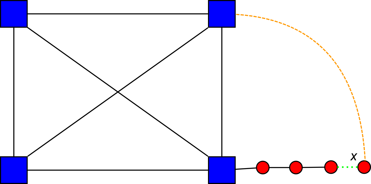
Figure 15: The suggested dynamics in Prop. 53. Here, $x=4$ and $m_{X}=4$. The link to the clique is dashed in orange, the canceled link is in dotted green.

The only possible deviation in this sub-graph is establishing additional links between a type-B player and clique members (other than the one it is currently linked to). This will only reduce the overall distance. Hence we can asymptotically bound the social cost by

$$\mathcal{S} < 3|T_{B}|^{2}+2|T_{B}||T_{A}|\left(A+1\right)$$

$$+2|T_{B}||T_{A}|c+|T_{A}|^{2}\left(c_{A}+A\right)$$

where the first term expresses the (maximal) distance between type-B nodes, the second the distance cost between the type-A clique and the type-B nodes, the third is the cost of links between type-A players and type-B players and the third is the cost of the type-A clique. Comparing this to the optimal solution (Proposition 45) under the assumption that $T_{B}>T_{A}$, we have

$$\mathcal{S}/\mathcal{S}_{optimal}<\frac{3}{2}+c.$$

This concludes the proof.

D) We can improve on the former bound by noting that according to Preference Order #2, when disconnecting from the long line a player will reconnect to the type-A player that has the least utility in his concern (and hence requires the lowest price). In other words, it will connect to one of the nodes that carry the least amount of type-B nodes at that moment. Therefore, to each type-A node roughly $|T_{B}|/|T_{A}|$ type-B nodes will be connected. This allows us to provide the following corollary.

According to the aforementioned discussion by establishing a link between node $j\in T_{B}$ and $i\in T_{A}$ (where $j$ in not connected directly to $i$) the change of cost is

$$\Delta C(i,ij) = c_{A}-A-\frac{|T_{B}|}{|T_{A}|}$$

$$\Delta C(j,ij) = c_{B}-1$$

but

$$\Delta C(i,ij)+\Delta C(j,ij)=2c-(A-1)-\frac{|T_{B}|}{|T_{A}|}>0$$

and the link would not be establish. Hence, we can neglect the term $2|T_{B}||T_{A}|c$ and

$$\sum C(i)<3|T_{B}|^{2}+2|T_{B}||T_{A}|\left(A+1\right)+|T_{A}|^{2}\left(c_{A}+A\right)$$

By comparing with the optimal solution we obtained the required result. ∎

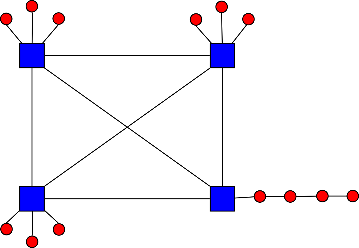
Figure 16: The network structure described in Prop. 53. The type-B players connect almost uniformly to the different members of the type-A clique. In addition, there is one line of type-B players.

In order to obtain the result in Proposition 45, we had to assume a large limit for the number of type-A players. Here, on the other hand, we were able to obtain a similar result yet without that assumption, i.e., solely by dynamic considerations.

It is important to note that, although our model allows for monetary transfers, in every resulting agreement between major players no monetary transaction is performed. In other words, our model predicts that the major players clique will form a settlement-free interconnection subgraph, while in major player - minor player contracts transactions will occur, and they will be of a transit contract type. Indeed, this observation is well founded in reality.

B.4 Detailed Calculations

In Proposition 9:

For the network presented in Fig. 2(a), the number of links in the type-A clique is the same as the number of pairs, which is ${|T_{A}|\choose 2}$. Each edge is counted twice at the social cost summation (as part of its members cost) and therefore the social cost due to the number of edges in the type-A clique is

$$2c{|T_{A}|\choose 2}=c|T_{A}|\left(|T_{A}|-1\right).$$

Likewise, the distance of each player in the type-A clique from every other type-A player is one, and the distance cost is counted twice, and we obtain the type-A clique distance cost term $A|T_{A}|\left(|T_{A}|-1\right)$.

As the distance between every two type-B players is 2, and there are ${|T_{B}|\choose 2}$ pairs, we obtain in a similar fashion the type-B to type-B distance cost term

$$2\cdot 2{|T_{B}|\choose 2}=2|T_{B}|\left(|T_{B}|-1\right).$$

There are $|T_{B}|$ type-B players and their distance to $|T_{A}|-1$ clique members is 2, and their distance to a single clique member is one. The distance is multiplied by $A$ when the sum is over a type-B player, and it is multiplied by $1$ when the sum is over a type-A player. Therefore, the social cost contribution of the type-A to type-B distance term is

$$2\left(A+1\right)|T_{B}|\left(|T_{A}|-1\right)+\left(A+1\right)|T_{B}|.$$

Finally, there are $|T_{B}|$ links connecting every type-B player to the clique, and each edge is summed twice, and we obtain the type-B players link’s cost

$$2c|T_{B}|.$$

If, however, one observes the network presented in Fig. 2(b), then every type-B players is connected by $|T_{A}|$ edges to the type-A clique. Therefore, the last two expressions are replaced,

$$\left(A+1\right)|T_{B}||T_{A}|+2c|T_{B}||T_{A}|$$

where the right term is the distance term and the second is the link’s cost term, and we have taken into account the double summation.

In Lemma 34:

For simplicity, assume $k$ is odd. Without the edge $(x_{k,}y_{\left(k+1\right)/2})$, the sum of distances from player $x_{k}$ to all players along the $(y_{1},y_{2},...y_{k})$ is

$$\sum_{i=k+1}^{2k}i=\frac{k\left(3k+1\right)}{2}$$

after the addition of the link $(x_{k,}y_{\left\lfloor\left(k+1\right)/2\right\rfloor})$, the the sum of distances is

$$2\sum_{i=1}^{\left(k+1\right)/2}i-1=\frac{k^{2}}{4}+k-\frac{1}{4}$$

and therefore the reduction is the sum of distances bounded from above by $5k^{2}/4$.

References

- Altman [1994] Altman, E. 1994. Flow control using the theory of zero sum Markov games. IEEE Trans. Automat. Controll 39, 4.
- Altman et al. [2000] Altman, E., Jimenez, T., Basar, T., and Shimkin, N. 2000. Competitive routing in networks with polynomial cost. In Proceedings IEEE INFOCOM 2000. Vol. 3. IEEE.
- Àlvarez and Fernàndez [2012] Àlvarez, C. and Fernàndez, A. 2012. Network Formation: Heterogeneous Traffic, Bilateral Contracting and Myopic Dynamics.
- Anshelevich et al. [2003] Anshelevich, E., Dasgupta, A., Tardos, E., and Wexler, T. 2003. Near-optimal network design with selfish agents. In Proc. thirty-fifth ACM Symp. Theory Comput. - STOC ’03. ACM Press, New York, New York, USA, 511.
- Anshelevich et al. [2011] Anshelevich, E., Shepherd, F., and Wilfong, G. 2011. Strategic network formation through peering and service agreements. Games and Economic Behavior 73, 1.
- Arcaute et al. [2013] Arcaute, E., Dyagilev, K., Johari, R., and Mannor, S. 2013. Dynamics in tree formation games. Games and Economic Behavior 79.
- Arcaute et al. [2009] Arcaute, E., Johari, R., and Mannor, S. 2009. Network Formation: Bilateral Contracting and Myopic Dynamics. IEEE Trans. Automat. Control 54, 8.
- Barabási [1999] Barabási, A. 1999. Emergence of Scaling in Random Networks. Science 286, 5439.
- Borkar and Manjunath [2007] Borkar, V. S. and Manjunath, D. 2007. Distributed topology control of wireless networks. Wireless Networks 14, 5.
- Charilas and Panagopoulos [2010] Charilas, D. E. and Panagopoulos, A. D. 2010. A survey on game theory applications in wireless networks. Computer Networks 54, 18.
- Chen et al. [2002] Chen, Q., Chang, H., Govindan, R., and Jamin, S. 2002. The origin of power laws in Internet topologies revisited. In INFOCOM 2002. Proceedings. IEEE. Vol. 2.
- Corbo and Parkes [2005] Corbo, J. and Parkes, D. 2005. The price of selfish behavior in bilateral network formation. In Proc. PODC ’05. ACM Press, New York, New York, USA, 99.
- Demaine et al. [2007] Demaine, E. D., Hajiaghayi, M., Mahini, H., and Zadimoghaddam, M. 2007. The price of anarchy in network creation games. In PODC. ’07. ACM Press.
- Fabrikant et al. [2003] Fabrikant, A., Luthra, A., Maneva, E., Papadimitriou, C. H., and Shenker, S. 2003. On a network creation game. In PODC ’03. ACM Press, 347–351.
- Gregori et al. [2013] Gregori, E., Lenzini, L., and Orsini, C. 2013. k-Dense communities in the Internet AS-level topology graph. Computer Networks 57, 1.
- Jackson and Wolinsky [1996] Jackson, M. O. and Wolinsky, A. 1996. A Strategic Model of Social and Economic Networks. Journal of Economic Theory 71, 1.
- Johari et al. [2006] Johari, R., Mannor, S., and Tsitsiklis, J. N. 2006. A contract-based model for directed network formation. Games and Economic Behavior 56, 2.
- Lazar et al. [1997] Lazar, A., Orda, A., and Pendarakis, D. 1997. Virtual path bandwidth allocation in multiuser networks. IEEE/ACM Trans. Netw. 5, 6.
- Lodhi et al. [2012] Lodhi, A., Dhamdhere, A., and Dovrolis, C. 2012. GENESIS: An agent-based model of interdomain network formation, traffic flow and economics. In 2012 Proc. IEEE INFOCOM. IEEE, 1197–1205.
- Meirom et al. [2013] Meirom, E. A., Mannor, S., and Orda, A. 2013. Formation Games and the Internet’s Structure. http://arxiv.org/abs/1307.4102.
- Nahir et al. [2009] Nahir, A., Orda, A., and Freund, A. 2009. Topology Design and Control: A Game-Theoretic Perspective. In INFOCOM 2009, IEEE.
- Nisan N. [2007] Nisan N., Roughgarden T., T. E. V. V., Ed. 2007. Algorithmic Game Theory. Cambridge University Press.
- Orda et al. [1993] Orda, A., Rom, R., and Shimkin, N. 1993. Competitive routing in multiuser communication networks. IEEE/ACM Trans. Netw. 1, 5.
- Roy et al. [2010] Roy, S., Ellis, C., Shiva, S., Dasgupta, D., Shandilya, V., and Wu, Q. 2010. A Survey of Game Theory as Applied to Network Security. HICSS 2010.
- Siganos et al. [2003] Siganos, G., Faloutsos, M., Faloutsos, P., and Faloutsos, C. 2003. Power laws and the AS-level internet topology. IEEE/ACM Trans. Netw. 11, 4.
- Vandenbossche and Demuynck [2012] Vandenbossche, J. and Demuynck, T. 2012. Network Formation with Heterogeneous Agents and Absolute Friction. Computational Economics.
- Vázquez et al. [2002] Vázquez, A., Pastor-Satorras, R., and Vespignani, A. 2002. Large-scale topological and dynamical properties of the Internet. Physical Review E 65, 6, 066130.

References

- [1] CAIDA AS Ranking, http://as-rank.caida.org/.
- Barabási [1999] Barabási, A. 1999. Emergence of Scaling in Random Networks. Science 286, 5439.
- Cohen and Havlin [2003] Cohen, R. and Havlin, S. 2003. Scale-Free Networks Are Ultrasmall. Phys. Rev. Lett. 90, 5, 058701.
- Gregori et al. [2011] Gregori, E., Improta, A., Lenzini, L., Rossi, L., and Sani, L. 2011. Bgp and inter-as economic relationships. In Proceedings of the 10th international IFIP TC 6 conference on Networking - Volume Part II. NETWORKING’11. Springer-Verlag, Berlin, Heidelberg.
- Meirom et al. [2013] Meirom, E. A., Mannor, S., and Orda, A. 2013. Formation Games and the Internet’s Structure.
- Pastor-Satorras et al. [2001] Pastor-Satorras, R., Vázquez, A., and Vespignani, A. 2001. Dynamical and Correlation Properties of the Internet. Phys. Rev. Lett. 87, 25, 258701.