Abstract

The holographic duals of higher spin theories on AdS₃ are described by the large $N$ limit of a family of minimal model CFTs, whose symmetry algebra is equivalent to ${\cal W}_{\infty}[\lambda]$. We study perturbations of these limit theories, and show that they possess a marginal symmetry-preserving perturbation that describes switching on the $\frac{1}{N}$ corrections. We also test our general results for the specific cases of $\lambda=0,1$, where free field realisations are available.

1 Introduction

The proposed dualities relating a higher spin theory on AdS_d+1 to vector-like nearly free conformal field theories in $d$ dimensions constitute simplified versions of the AdS/CFT correspondence that are under very good quantitative control. As such they may open the way towards understanding their inner workings. The prototype example was proposed some years ago by Klebanov & Polyakov [1], see also [2, 3, 4, 5] for earlier work and [6] for a subsequent generalisation. It relates a Vasiliev higher spin theory [7] on AdS₄ to the large $N$ limit of the ${\rm O}(N)$ vector model in $3$ dimensions. Compelling evidence for this duality was recently found by comparing correlation functions in [8, 9], as well as through the work [10, 11] that determined interesting general constraints on the structure of the correlation functions based on symmetry considerations. More recently, these dualities were further generalised to a one-parameter family of (in general) parity-breaking theories in [12, 13, 14].

In a somewhat independent development, a lower dimension analogue of this duality was proposed in [15], relating a higher spin theory on AdS₃ [16, 17] to the large $N$ limit of a family of minimal model 2d CFTs. One of the guiding principles in proposing this duality was the observation that the asymptotic algebra of the higher spin theory on AdS₃ is described by a ${\cal W}_{\infty}[\lambda]$ algebra [18, 19, 20, 21], which therefore largely controls the dual CFT. This proposal was subsequently checked in various ways [22, 23].

In the 3d/2d case, the underlying symmetry algebra ${\cal W}_{\infty}[\lambda]$ is characterised, in addition to the central charge (that corresponds geometrically to the size of the AdS space), by a continuous parameter $\lambda$ that controls the higher spin interactions. From the dual minimal model perspective, $\lambda$ is identified with

$$\lambda=\frac{N}{N+k}\ ,\qquad\hbox{while}\quad c=(N-1)\Bigl{[}1-\frac{N(N+1)}{(N+k)(N+k+1)}\Bigr{]}\ ,$$ (1.1)

where $k$ is the level of the coset model. In particular, $\lambda$ therefore becomes a continuous parameter in the ’t Hooft limit, in which $c\sim N(1-\lambda^{2})$. However, from the viewpoint of the ${\cal W}_{\infty}[\lambda]$ symmetry algebra, $\lambda$ and $c$ are arbitrary (finite) parameters, and there is a priori no need to take $c\rightarrow\infty$ in order for $\lambda$ to become continuous.

It is then natural to ask whether theories corresponding to different values of $\lambda$ (and $c$) are connected by continuous deformations. For example, one may wonder whether there exist exactly marginal operators that change $\lambda$ continuously (while preserving the ${\cal W}_{\infty}$ symmetry) without affecting $c$. Or there could be deformations that change both $\lambda$ and $c$ infinitesimally. Given that the ${\cal W}_{N,k}$ minimal models do not possess any exactly marginal operators, one may suspect that the first option is not possible, and indeed there is a fairly general argument — due to Stefan Fredenhagen — that implies that such deformations cannot exist. (This will be briefly reviewed in section 5.1.) However, we find evidence that a marginal deformation exists, at least in the ’t Hooft limit, that modifies both $\lambda$ and $c$. In fact, it can be identified with a perturbation that introduces $\frac{1}{N}$ and $\frac{1}{k}$ corrections such that to first order $\lambda$ does not change.

More specifically, we characterise quite generally the perturbing operators that preserve the ${\cal W}_{\infty}$ symmetry to first order, and find that there is a one-parameter family of operators with this property. They are uniquely characterised by their eigenvalues of the spin-$3$ generator. Quite remarkably, the $h=1$ descendant of the light state corresponding to $(\tiny\yng(1);\tiny\yng(1))$ has this property in the ’t Hooft limit and therefore defines (together with its conjugate operator) an interesting perturbing field. We analyse its properties, first for the special cases $\lambda=0,1$, where free field realisations are available, and then for general $\lambda$, using conformal perturbation theory. The conformal perturbation theory is quite intricate since, in the ’t Hooft limit, there are infinitely many fields of the same conformal dimension, and hence we need to analyse an infinitely degenerate case. However, because of the structure of the fusion rules, the perturbation problem has a lot of structure, and we can identify at least certain qualitative features.

The paper is organised as follows. We begin with reviewing the free field realisations of the special ${\cal W}_{\infty}[\lambda]$ theories at $\lambda=0$ (section 2) and $\lambda=1$ (section 3). In particular, we show that the singlet sector of $N$ complex free fermions defines a ${\cal W}_{\infty}[0]$ algebra at $c=N-1$, while the singlet sector of $k$ complex free bosons lead to ${\cal W}_{\infty}[1]$ at $c=2k$. While both of these statements are certainly expected, they had not been established at finite $c$ before; in particular, we confirm that the structure constants of the ${\cal W}_{\infty}[\lambda]$ algebras agree precisely with the prediction of [23] for these values of $\lambda$ and $c$. In section 4 we then study the conditions a perturbing operator must satisfy in order to preserve the ${\cal W}_{\infty}$ algebra at first order. This is first done in the ’t Hooft limit, and then for finite $c$, using the full quantum version of the ${\cal W}_{\infty}[\lambda]$ algebra. We give strong evidence that the $h=1$ descendant of the light state corresponding to $(\tiny\yng(1);\tiny\yng(1))$ has this property in the ’t Hooft limit, and confirm this statement explicitly for the special cases $\lambda=0$ and $\lambda=1$ (where the statement remains true even at finite $c$). In section 5 we then study the effect of the perturbation by this field (and its conjugate) in the ’t Hooft limit, and identify the perturbed spectrum with what is obtained from the minimal model perspective upon switching on a certain combination of $\frac{1}{N}$ and $\frac{1}{k}$ corrections. Finally, we conclude in section 6. There are four appendices where some of the more technical material has been collected together.

2 The theory at $\lambda=0$

The simplest explicit realisation of the ${\cal W}_{\infty}[\lambda]$ algebra exists at $\lambda=0$, where we can describe the theory in terms of free fermions. We shall later also comment on how this description is related to the continuous orbifold point of view proposed in [24].

2.1 The free fermion description

Let us consider the theory of $N$ free complex fermions $\psi^{i}$ and $\psi^{*i}$, $i=1,\ldots,N$ with action

$$S_{0}=\int d^{2}z\left(\psi^{*i}\,\bar{\partial}\psi^{i}+\bar{\psi}^{i}\,\partial\bar{\psi}^{*i}\right)\ .$$ (2.1)

The corresponding equations of motion are

$$\bar{\partial}\psi^{i}=\bar{\partial}\psi^{*i}=0\ ,$$ (2.2)

and the OPEs take the form

$$\psi^{i}(z_{1})\,\psi^{\ast j}(z_{2})\sim\frac{\delta^{ij}}{(z_{1}-z_{2})}\ ,$$ (2.3)

with similar expressions for the right movers $\bar{\psi}^{i}$ and $\bar{\psi}^{*j}$. We shall always consider only states that are singlets with respect to the global ${\rm SU}(N)$ action.

The free theory has the conserved spin-$s$ chiral currents [25, 26, 27] (the expressions for the anti-chiral currents are analogous)

$$W^{s}=n(s)\sum^{s-1}_{k=0}(-1)^{k}\binom{s-1}{k}^{2}\,\partial^{s-1-k}\psi^{*i}\,\partial^{k}\psi^{i}\ ,$$ (2.4)

where the sum over $i$ is implicit, and we choose the normalisation convention

$$n(s)=\frac{[(s-1)!]^{2}}{(2s-2)!}\ .$$ (2.5)

Explicitly, for small values of $s$, these current are then

$$J \equiv W^{1}=\psi^{*i}\psi^{i}$$ (2.6)

$$T \equiv W^{2}=\frac{1}{2}(\partial\psi^{*i}\,\psi^{i}-\psi^{*i}\,\partial\psi^{i})$$ (2.7)

$$W \equiv W^{3}=\frac{1}{6}\Bigl{(}\partial^{2}\psi^{*i}\,\psi^{i}-4\,\partial\psi^{*i}\,\partial\psi^{i}+\psi^{*i}\,\partial^{2}\psi^{i}\Bigr{)}$$ (2.8)

$$U \equiv W^{4}=\frac{1}{20}\Bigl{(}\partial^{3}\psi^{\ast i}\,\psi^{i}-9\,\partial^{2}\psi^{\ast i}\,\partial\psi^{i}+9\,\partial\psi^{\ast i}\,\partial^{2}\psi^{i}-\psi^{\ast i}\,\partial^{3}\psi^{i}\Bigr{)}\ .$$ (2.9)

2.2 OPEs and commutation relations

It follows from the OPEs given in Appendix A that the modes of the stress energy tensor $T$ satisfy a Virasoro algebra with central charge $c=N$,

$${}[L_{m},L_{n}]=(m-n)L_{m+n}+\frac{N}{12}m\,(m^{2}-1)\,\delta_{m,-n}\ ,$$ (2.10)

while $J$ is a ${\rm U}(1)$-current whose modes satisfy

$$[J_{m},J_{n}]=N\,m\,\delta_{m,-n}\ ,\qquad[L_{m},J_{n}]=-n\,J_{m+n}\ .$$ (2.11)

It also follows from (A.5) and (A.6) that $W$ is neither ${\rm U}(1)$- nor Virasoro-primary. Indeed, converted into modes, these OPEs imply that the commutation relations take the form

$${}[J_{m},W_{n}]=2mL_{m+n}\ ,\qquad[L_{m},W_{n}]=(2m-n)W_{m+n}+\tfrac{1}{6}m(m^{2}-1)J_{m+n}\ .$$ (2.12)

The OPE of $W$ with itself (A.7) then leads to

$${}[W_{m},W_{n}] = \tfrac{2N}{360}\,m(m^{2}-1)(m^{2}-4)\delta_{m,-n}+\tfrac{1}{15}(m-n)(2m^{2}+2n^{2}-mn-8)L_{m+n}$$ (2.13)

$$+2(m-n)U_{m+n}\ .$$

Note that this algebra is linear, i.e. the commutators (2.13) do not involve the normal ordered $\Lambda^{(4)}=:LL:$ term that generically appears in this commutator.

2.3 The ${\rm U}(1)$ coset

The free fermion theory does not directly describe ${\cal W}_{\infty}[\lambda]$ for any value of $\lambda$, since it contains a spin $1$ current $J$, and hence leads to ${\cal W}_{1+\infty}$. Furthermore, in the above basis (in which the generators are bilinears in the fermions, and hence the OPEs do not contain any non-linear term) the generators $W^{s}$ with $s\geq 2$ do not close among themselves, as follows for example from (A.6). There is, however, a different basis in which ${\cal W}_{\infty}[0]$ appears as a subalgebra of the free fermion theory. In this basis, the generators are not just bilinears in the free fermions, and as a consequence the algebra will turn out to be non-linear.

The basic idea for finding this basis is inspired by the coset construction, and in effect, the resulting construction is what the coset by the ${\rm U}(1)$-current $J$ would amount to. We can recursively construct currents $\tilde{W}^{s}$ of spin $s=2,3,\ldots$ that are primary with respect to $J$. In terms of modes this then means that the modes $\tilde{W}^{s}_{m}$ commute with $J_{n}$. Because of the Jacobi identity, the same is then also true for the commutators of $\tilde{W}^{s_{1}}$ and $\tilde{W}^{s_{2}}$, i.e. the $\tilde{W}^{s}$ generators form a closed algebra. In the following we shall construct the first few of these generators explicitly; we can then determine their commutation relations, and show that they generate indeed ${\cal W}_{\infty}[0]$ at $c=N-1$.

2.3.1 The coset generators

Let us first define the generators $\tilde{W}_{s}$ recursively. For $s=2$, we get

$$\tilde{T}=T-\frac{1}{2N}:JJ:\ ,$$ (2.14)

or in terms of states

$$\tilde{L}_{-2}\Omega=L_{-2}\Omega-\frac{1}{2N}J_{-1}J_{-1}\Omega\ .$$ (2.15)

It is easy to see that (2.15) is ${\rm U}(1)$-primary, i.e.  $J_{n}\tilde{L}_{-2}\Omega=0$ for $n\geq 0$. The OPEs of $\tilde{T}$ with $J$ and itself are then

$$\tilde{T}(z_{1})J(z_{2})\sim 0\ ,\qquad\tilde{T}(z_{1})\tilde{T}(z_{2})\sim\frac{(N-1)/2}{(z_{1}-z_{2})^{4}}+\frac{2\tilde{T}(z_{2})}{(z_{1}-z_{2})^{2}}+\frac{\tilde{T}^{\prime}(z_{2})}{(z_{1}-z_{2})}\ ,$$ (2.16)

i.e. the new modes $\tilde{L}_{n}$ define a Virasoro algebra (2.10) with central charge $N-1$ (instead of $N$), and commute with the modes $J_{n}$.

For $s=3$, the ${\rm U}(1)$-primary generator is

$$\tilde{W}=W-\frac{2}{N}:JT:+\frac{2}{3N^{2}}\,:JJJ:\ ,$$ (2.17)

or in terms of states

$$\tilde{W}_{-3}\Omega=W_{-3}\Omega-\frac{2}{N}\,J_{-1}L_{-2}\Omega+\frac{2}{3N^{2}}\,J_{-1}J_{-1}J_{-1}\Omega\ .$$ (2.18)

Moreover, $\tilde{W}$ is also primary with respect to $\tilde{T}$, i.e.

$$\tilde{T}(z_{1})\tilde{W}(z_{2})\sim\frac{3\tilde{W}(z_{2})}{(z_{1}-z_{2})^{2}}+\frac{\tilde{W}^{\prime}(z_{2})}{(z_{1}-z_{2})}\ ,$$ (2.19)

which in particular does not involve the current $J$ any longer, in contrast to the situation in (A.6), and in agreement with the above general argument. Incidentally, the simplest way to compute (2.19) is to use the general formula

$$\tilde{T}(z_{1})\tilde{W}(z_{2})=\sum_{n\in\mathbb{Z}}\,(z_{1}-z_{2})^{-n-2}V\bigl{(}\tilde{L}_{n}\tilde{W}_{-3}\Omega,z_{2}\bigr{)}\ ,$$ (2.20)

where $V(\psi,z)$ denotes the vertex operator associated to $\psi$, together with the mode expansion of $\tilde{T}$,

$$\tilde{L}_{n}=L_{n}-\frac{1}{2N}\sum_{l\in\mathbb{Z}}:J_{n-l}J_{l}:\ .$$ (2.21)

We also need the explicit formula for the ${\rm U}(1)$-primary state at $h=4$, which equals

$$\tilde{U}_{-4}\Omega = U_{-4}\Omega-\frac{1}{5N}J_{-1}J_{-3}\Omega-\frac{3}{20N}J_{-2}J_{-2}\Omega-\frac{3}{N}J_{-1}W_{-3}\Omega+\frac{3}{N^{2}}J_{-1}J_{-1}L_{-2}\Omega$$ (2.22)

$$-\frac{3}{4N^{3}}J_{-1}J_{-1}J_{-1}J_{-1}\Omega-\frac{(21-\frac{15}{N})}{(5N+17)}\,(\tilde{L}_{-2}\tilde{L}_{-2}-\tfrac{3}{5}\tilde{L}_{-4})\Omega\ ,$$

where the last term is required in order to make it also Virasoro primary with respect to $\tilde{T}$.

Continuing in this manner, we can recursively construct ${\rm U}(1)$-primary fields $\tilde{W}^{s}$ that generate a closed algebra. We can furthermore recursively make them Virasoro primary (with respect to $\tilde{T}$), and thus the resulting ${\cal W}_{\infty}$ algebra has the spin content $2,3,4,\ldots$. Following the general logic of [23], it must therefore be isomorphic to ${\cal W}_{\infty}[\lambda]$ for some value of $\lambda$. In the following we shall show that the relevant value of $\lambda$ is $\lambda=0$. Note that the classical analysis of [20] only tells us that this has to be true to leading order in $1/c$; now we have shown that it is actually true even at finite $c=N-1$.

2.3.2 Determining $\lambda$

In order to determine the value of the parameter $\lambda$, it is sufficient to calculate two commutators. Indeed, in the conventions of [23] and [28], we have

$${}[\tilde{W}_{m},\tilde{W}_{n}] = \frac{N_{3}c}{144}\,m(m^{2}-1)(m^{2}-4)\delta_{m,-n}+\frac{N_{3}}{12}(m-n)(2m^{2}+2n^{2}-mn-8)\tilde{L}_{m+n}$$ (2.23)

$$+2(m-n)\tilde{U}_{m+n}+\frac{40\,N_{3}}{(5c+22)}(m-n)\tilde{\Lambda}_{m+n}\ ,$$

$${}[\tilde{U}_{m},\tilde{U}_{n}] = \frac{N_{4}c}{4320}\,m(m^{2}-1)(m^{2}-4)(m^{2}-9)\delta_{m,-n}+\cdots\ ,$$ (2.24)

and the parameter $\gamma^{2}$, which determines the coefficient of $U$ in the $WW$ OPE [23] and characterises the ${\cal W}$ algebra uniquely, is then given by

$$\gamma^{2}=\frac{896}{75}\,\frac{N_{4}}{N_{3}^{2}}\ .$$ (2.25)

Using the analogue of (2.20), we have worked out the first few terms of the $\tilde{W}\tilde{W}$ OPE to be

$$\tilde{W}(z_{1})\,\tilde{W}(z_{2}) \sim \frac{2(N-1)(N-2)}{3N}\,\frac{1}{(z_{1}-z_{2})^{6}}+\frac{4(N-2)}{N}\frac{\tilde{T}(z_{2})}{(z_{1}-z_{2})^{4}}+\frac{2(N-2)}{N}\frac{\tilde{T}^{\prime}(z_{2})}{(z_{1}-z_{2})^{3}}$$ (2.26)

$$+\frac{4\,\tilde{U}(z_{2})+\frac{3}{5}\,\tilde{T}^{\prime\prime}(z_{2})}{(z_{1}-z_{2})^{2}}+\frac{64(N-2)}{5N(N-1)}\frac{\tilde{\Lambda}^{(4)}(z_{2})}{(z_{1}-z_{2})^{2}}+{\cal O}\left(\frac{1}{z_{1}-z_{2}}\right)\ ,$$

where $\tilde{\Lambda}^{(4)}$ is the composite field $\tilde{\Lambda}^{(4)}=:\tilde{T}\tilde{T}:-\frac{3}{10}\partial^{2}\tilde{T}$. Comparing with the central term in (2.23) and using that $c=N-1$, we conclude that

$$N_{3}=\frac{4}{5}\frac{N-2}{N}\ .$$ (2.27)

In order to compute $N_{4}$, we have also determined the central term in the $\tilde{U}\tilde{U}$ OPE, i.e.

$$\tilde{U}_{4}\tilde{U}_{-4}\Omega=\frac{9(N-1)(N-2)(N-3)(N+1)}{N^{2}(5N+17)}\,\Omega\ ,$$ (2.28)

which gives

$$N_{4}=\frac{54}{7}\,\frac{(N-2)(N-3)(N+1)}{N^{2}(5N+17)}\ .$$ (2.29)

Thus $\gamma^{2}$ becomes

$$\gamma^{2}=\frac{144(N+1)(N-3)}{(5N+17)(N-2)}=\left.\frac{64(c+2)(\lambda-3)\bigl{(}c(\lambda+3)+2(4\lambda+3)(\lambda-1)\bigr{)}}{(5c+22)(\lambda-2)\bigl{(}c(\lambda+2)+(3\lambda+2)(\lambda-1)\bigr{)}}\right|_{\lambda=0,c=N-1}\ ,$$ (2.30)

i.e. it agrees with the general formula of [23, eq. (2.15)] at $\lambda=0$ and $c=N-1$. This proves that the free fermion construction indeed gives rise to ${\cal W}_{\infty}[\lambda=0]$ at $c=N-1$.

We should mention that this argument relies on the assumption that the only consistent ${\cal W}_{\infty}$ algebras that are generated by one field of each integer spin $s\geq 2$ are described by ${\cal W}_{\infty}[\lambda]$. While this statement has not been established in complete generality, there is very convincing evidence, based on the analysis of [29], that this is indeed the case.

2.4 The continuous orbifold viewpoint

It was argued in [24] that the theory at $\lambda=0$ can be described in terms of a continuous orbifold. More specifically, one considers the affine $\hat{\mathfrak{su}}(N)_{1}$ theory, and takes the orbifold by the action of the group ${\rm SU}(N)/\mathbb{Z}_{N}$. In the untwisted sector this amounts to restricting the affine level $1$ theory to those states that are ${\rm SU}(N)/\mathbb{Z}_{N}$ singlets. From this point of view, the higher spin currents then arise from the Casimir operators; in particular, the stress energy tensor of the continuous orbifold theory equals

$$T^{{\rm co}}=\frac{1}{2(N+1)}\,\sum_{a}:J^{a}J^{a}:\ ,$$ (2.31)

where $J^{a}$ are the currents of the $\hat{\mathfrak{su}}(N)_{1}$ theory, while the spin $3$ generator is

$$W^{\rm co}=\frac{1}{3(N+1)(N+2)}\,\sum_{abc}d_{abc}:J^{a}J^{b}J^{c}:\ ,$$ (2.32)

where $d_{abc}$ is the totally symmetric invariant tensor. The higher spin generators are similarly associated to the higher order Casimir operators.

Actually, the relation between this continuous orbifold description and the free fermion construction from above is fairly immediate. The theory of $N$ complex fermions has a $\hat{\mathfrak{u}}(N)_{1}$ algebra, whose generators are

$$J^{ij}=\psi^{\ast\,i}\psi^{j}\ .$$ (2.33)

This current algebra contains the $\hat{\mathfrak{u}}(1)$ subalgebra generated by $J=\sum_{i}\psi^{\ast\,i}\psi^{i}$ and the coset by this $\hat{\mathfrak{u}}(1)$ algebra (see section 2.3) leads to an affine $\hat{\mathfrak{su}}(N)_{1}$ theory at $c=N-1$. Indeed, the $\hat{\mathfrak{su}}(N)_{1}$ currents are simply given by, see [30, chapter 15.5.6]

$$J^{a}=\sum_{ij}\psi^{\ast i}\,t^{a}_{ij}\,\psi^{j}\ ,$$ (2.34)

where $t^{a}_{ij}$ are the generators of $\mathfrak{su}(N)$ in the fundamental representation. In both theories we are furthermore considering only singlets with respect to the global ${\rm SU}(N)$ action, and thus the spectra agree precisely (in the untwisted sector). The twisted sectors are then completed by consistency, and thus should also match. (It might be interesting to understand the twisted sectors more directly from the free fermion point of view; this could be closely related to the discussion of [31] in one dimension higher.)

Using the translation between the free fermion and the $\hat{\mathfrak{su}}(N)_{1}$ description, it was shown in [30, chapter 15.5.6] that the stress energy tensor of (2.31) agrees indeed with $\tilde{T}$ from (2.14). We have also checked that (2.32) and (2.17) similarly agree.

3 The theory at $\lambda=1$

The other simple realisation of the ${\cal W}_{\infty}[\lambda]$ algebra arises for $\lambda=1$, for which there is a description in terms of $k$ complex free bosons.

3.1 The higher spin currents

The theory of $k$ complex free bosons has spin-$s$ currents [32]

$$W^{s}(z)=m(s)\sum_{l=1}^{s-1}\,\frac{(-1)^{l}}{(s-1)}\left({s-1\atop l}\right)\left({s-1\atop s-l}\right)\,\partial^{l}\phi^{\,j}\,\,\partial^{s-l}\bar{\phi}^{\,j}\ ,$$ (3.1)

where the sum over $j=1,\ldots,k$ is implicit, and we choose the normalization factor

$$m(s)=\frac{2^{s-3}s!}{(2s-3)!!}\ .$$ (3.2)

Explicitly, the first few currents are

$$T(z) \equiv W^{2}(z)=-:\partial\phi^{\,j}\,\partial\bar{\phi}^{\,j}:$$ (3.3)

$$W(z) \equiv W^{3}(z)=-2:(\partial\phi^{\,j}\,\partial^{2}\bar{\phi}^{\,j}-\partial^{2}\phi^{\,j}\,\partial\bar{\phi}^{\,j}):$$ (3.4)

$$U(z) \equiv W^{4}(z)=-\frac{16}{5}:(\partial\phi^{\,j}\,\partial^{3}\bar{\phi}^{\,j}-3\,\partial^{2}\phi^{\,j}\,\partial^{2}\bar{\phi}^{\,j}+\partial^{3}\phi^{\,j}\,\partial\bar{\phi}^{\,j}):\ .$$ (3.5)

Using the OPEs of the currents

$$\partial\phi^{\,i}(z_{1})\,\partial\bar{\phi}^{\,j}(z_{2})\sim-\frac{\delta^{ij}}{(z_{1}-z_{2})^{2}}$$ (3.6)

we can work out the OPEs of higher spin currents, and one finds for the stress energy tensor

$$T(z_{1})T(z_{2})=\frac{k}{(z_{1}-z_{2})^{4}}+\frac{2T(z_{2})}{(z_{1}-z_{2})^{2}}+\frac{\partial T(z_{2})}{(z_{1}-z_{2})}+\cdots\ ,$$ (3.7)

thus showing that the central charge equals $c=2k$, as expected. Some of the other OPEs are worked out explicitly in Appendix B, see eqs. (B.1) – (B.5); converted into modes, they give rise to the commutation relations

$$[L_{m},L_{n}] = (m-n)L_{m+n}+\tfrac{k}{6}m(m^{2}-1)\delta_{m+n}$$ (3.8)

$$[L_{m},W_{n}] = (2m-n)W_{m+n}$$ (3.9)

$$[L_{m},U_{n}] = (3m-n)U_{m+n}+\tfrac{32}{5}m(m^{2}-1)L_{m+n}$$ (3.10)

$$[W_{m},W_{n}] = 2(m-n)U_{m+n}+\tfrac{4}{5}(m-n)(2m^{2}+2n^{2}-mn-8)L_{m+n}$$ (3.12)

$$+\tfrac{2k}{15}m(m^{2}-1)(m^{2}-4)\delta_{m+n}$$

$$[W_{m},U_{n}] = (3m-2n)X_{m+n}+\tfrac{64}{35}(5m^{3}-5m^{2}n+3mn^{2}-17m-n^{3}+9n)W_{m+n}$$

$$[U_{m},U_{n}] = \tfrac{64}{525}km(m^{2}-1)(m^{2}-4)(m^{2}-9)\delta_{m+n}+\cdots\ ,$$ (3.13)

where we have only worked out the leading term for the $[U,U]$ commutator.

3.2 The primary basis

The $W^{s}$ as defined in (3.1) are not primaries: while $W^{3}$ is still a primary (see (3.9)), the spin-$4$ field $U$ is already not primary (see eq. (3.10)). In order to identify the $\lambda$ value of the resulting algebra, it is convenient to go to a primary basis. For instance, the spin-$4$ current in the primary basis is

$$\tilde{U}=U-\frac{192}{10k+22}\,\Lambda^{(4)}\ ,$$ (3.14)

where $\Lambda^{(4)}\left(=:TT:-\frac{3}{10}\partial^{2}T\right)$ is the familiar composite field, see eq. (2.26). In terms of this field, the relevant OPEs then become

$$W(z_{1})W(z_{2}) = \frac{16k}{z_{12}^{6}}+48\left[\frac{T}{z_{12}^{4}}+\frac{1}{2}\frac{\partial T}{z_{12}^{3}}+\frac{3}{20}\frac{\partial^{2}T}{z_{12}^{2}}+\frac{1}{30}\frac{\partial^{3}T}{z_{12}}\right]$$ (3.15)

$$+\frac{4}{z_{12}^{2}}\left[\tilde{U}+\frac{192}{10k+22}\Lambda^{(4)}\right]+\frac{2}{z_{12}}\left[\partial\tilde{U}+\frac{192}{10k+22}\partial\Lambda^{(4)}\right]\ ,$$

$$\tilde{U}(z_{1})\tilde{U}(z_{2}) = \frac{3072(2k+2)k}{10k+22}\frac{1}{z_{12}^{8}}+\cdots\ .$$ (3.16)

Comparing as before with eqs. (2.23) and (2.24) we thus conclude that

$$N_{3}=\frac{48}{5}\ ,\qquad N_{4}=\frac{9216}{7}\,\frac{c+2}{5c+22}\ ,$$ (3.17)

where we have used that $c=2k$. Thus the $\gamma^{2}$ parameter from eq. (2.25) becomes

$$\gamma^{2}=\frac{512(c+2)}{3(5c+22)}=\left.\frac{64(c+2)(\lambda-3)(c(\lambda+3)+2(4\lambda+3)(\lambda-1))}{(5c+22)(\lambda-2)(c(\lambda+2)+(3\lambda+2)(\lambda-1))}\right|_{\lambda=1}\ .$$ (3.18)

Hence the free boson theory generates indeed ${\cal W}_{\infty}[\lambda=1]$ at $c=2k$. Moreover, the seemingly non-linear ${\cal W}_{\infty}[\lambda=1]$ algebra of eq. (3.15) is in fact linear upon going to the original non-primary basis (3.1), in agreement with the analysis of [20].

4 Deforming the theory

We are interested in perturbing the ${\cal W}_{\infty}[\lambda]$ algebra by a marginal operator that preserves the current symmetry, i.e. by a perturbation that leaves all currents of ${\cal W}_{\infty}[\lambda]$ holomorphic. From the analysis of [33], see also [34], we know that to first order in perturbation theory this will be the case provided that

$$\lim_{\epsilon\rightarrow 0}\oint_{|w-z|=\epsilon}dw\,\Phi(w,\bar{w})W^{s}(z)=0\ .$$ (4.1)

Since we know that the OPE of $W^{s}$ with $\Phi$ is of the form

$$W^{s}(z)\Phi(w,\bar{w})=\sum_{l}(W^{s}_{l}\Phi)(w,\bar{w})\,(z-w)^{-l-s}$$ (4.2)

the requirement that $W^{s}$ remains holomorphic means that

$${\cal N}_{s}\equiv\sum_{l=0}^{s-1}\frac{(-1)^{l}}{l!}\,(L_{-1})^{l}\,W^{s}_{-s+1+l}\,\Phi=0\qquad s\geq 2\ .$$ (4.3)

(Here we have assumed that $\Phi$ is ${\cal W}_{\infty}[\lambda]$ primary.) Given that the ${\cal W}_{N,k}$ minimal models are not expected to have any such perturbation — the integrable perturbation by the field $(0;{\rm adj})$ is relevant and induces the RG flow from $k\rightarrow k-1$ — we can only hope to find a solution to this problem either at generic values of $(\lambda,c)$ of the ${\cal W}_{\infty}[\lambda]$ theory, or in the ’t Hooft limit of the ${\cal W}_{N,k}$ models. Remarkably, there is a simple perturbing field $\Phi$ that seems to satisfy (4.3) in the ’t Hooft limit, as we shall now explain.

4.1 The perturbation in the ’t Hooft limit

We begin by analysing the condition (4.3) in the ’t Hooft limit, i.e. in the limit of the minimal models ${\cal W}_{N,k}$ where we take $N,k\rightarrow\infty$ while keeping

$$\lambda=\frac{N}{N+k}$$ (4.4)

fixed. It was shown in [23] that with the central charge

$$c_{N,k}=(N-1)\Bigl{[}1-\frac{N(N+1)}{(N+k)(N+k+1)}\Bigr{]}$$ (4.5)

the chiral algebra ${\cal W}_{N,k}\cong{\cal W}_{\infty}[\lambda]$, even at finite $N$ and $k$. In the ’t Hooft limit $c_{N,k}\rightarrow\infty$, and hence the non-linear terms in ${\cal W}_{\infty}[\lambda]$ drop out. Let us denote the eigenvalues of the ${\cal W}_{\infty}[\lambda]$ primary state $\Phi$ by

$$W^{t}_{0}\Phi=w^{t}\Phi\qquad t\geq 2\ .$$ (4.6)

By construction ${\cal N}_{2}=0$ provided that $\Phi$ is marginal, i.e. $w^{2}\equiv h=1$. On the other hand, the ${\cal N}_{s}$ with $s\geq 3$ are generically non-trivial null-vectors. In order to confirm that they are indeed null we need to show that they are annihilated by all positive ${\cal W}_{\infty}[\lambda]$ modes. Using the commutation relations $[L_{m},W^{s}_{n}]=((s-1)m-n)\,W^{s}_{m+n}$ one can easily check that

$$L_{n}\,{\cal N}_{s}=0\qquad n\geq 1\ ,\ s\geq 3\ .$$ (4.7)

Thus it is sufficient to require

$$W^{s}_{n}\,{\cal N}_{t}=0\ ,\qquad s,t\geq 3\ ,\ \ n\geq 1\ .$$ (4.8)

We now consider the special case of (4.8) with $s=3$ and $n=t-1$. Then using the structure of the commutation relations of ${\cal W}_{\infty}[\lambda]$, in particular the fact that the highest spin mode that appears in the commutator of $W^{3}$ with $W^{t}$ is $W^{t+1}$, (4.8) leads to an equation for the eigenvalue $w^{t+1}$ in terms of the eigenvalues $w^{s}$ with $s\leq t$ (as well as the structure constants of the algebra). For example, from (4.8) with $s=3$ and $n=t-1=2$ with $t=3,4,5$ we obtain

$$w^{4} = \frac{3}{4}\Bigl{(}N_{3}+(w^{3})^{2}\Bigr{)}$$ (4.9)

$$w^{5} = \frac{1}{15}\Bigl{(}10\,w^{4}\,w^{3}+8\,\frac{N_{4}}{N_{3}}\,w^{3}\Bigr{)}$$ (4.10)

$$w^{6} = \frac{1}{9}\Bigl{(}5\,(w^{4})^{2}+30\,n_{44}\,w^{4}-3N_{4}\Bigr{)}\ ,$$ (4.11)

where $N_{3}$, $N_{4}$ and $n_{44}$ are the structure constants of the ${\cal W}_{\infty}[\lambda]$ algebra, which equal, in our conventions,

$$N_{3}=\frac{16}{5}\,\sigma^{2}(\lambda^{2}-4)\ ,\quad N_{4}=\frac{384}{35}\,\sigma^{4}(\lambda^{2}-4)(\lambda^{2}-9)\ ,\quad n_{44}=\frac{8}{15}\,\sigma^{2}\,(\lambda^{2}-19)\ ,$$ (4.12)

where $\sigma$ is a normalisation constant.

Thus this subset of conditions fixes the eigenvalues of $\Phi$ up to an arbitrary choice of $w^{3}$. One might wonder whether some of the other conditions in (4.8) would then fix $w^{3}$, but this does not seem to be the case. In fact there is an intuitive reason why this should be so: the set of conditions (4.8) with $s=3$ and $n=t-1$ is equivalent to the set of conditions with $t=3$, $n=1,2$ and $s=3,4,\ldots$. On the other hand, these latter conditions are equivalent to the statement that ${\cal N}_{3}$ is indeed a null-vector, i.e. to the statement that the $W^{3}$-current remains holomorphic to first order in perturbation. But since the whole ${\cal W}_{\infty}[\lambda]$ algebra is generated by repeated OPEs from $W^{3}$, this should then imply that the whole ${\cal W}_{\infty}[\lambda]$ algebra remains holomorphic to first order, i.e. (4.8) is satisfied for all $s,t\geq 3$ and $n\geq 1$.

This suggests that a one-parameter family of representations preserve the ${\cal W}_{\infty}[\lambda]$ algebra to first order in perturbation theory. One might then wonder whether one of the coset fields would satisfy these constraints in the ’t Hooft limit. Quite remarkably, this does seem to be the case. To see how this goes, recall that the $(\tiny{\yng(1)};\tiny{\yng(1)})$ representation becomes indecomposable in the ’t Hooft limit, i.e. its structure is [22]

$$({\tiny{\yng(1)}};{\tiny{\yng(1)}}):\qquad\lx@xy@svg{\hbox{\raise 0.0pt\hbox{\kern 11.69168pt\hbox{\ignorespaces\ignorespaces\ignorespaces\hbox{\vtop{\kern 0.0pt\offinterlineskip\halign{\entry@#!@&&\entry@@#!@\cr&&&&&&&\\&&&&&&&\\&&&&&&&\\&&&&&&&\crcr}}}\ignorespaces{\hbox{\kern-3.0pt\raise 0.0pt\hbox{\hbox{\kern 0.0pt\raise 0.0pt\hbox{\hbox{\kern 3.0pt\raise 0.0pt\hbox{$\textstyle{}$}}}}}}}{\hbox{\kern 23.69168pt\raise 0.0pt\hbox{\hbox{\kern 0.0pt\raise 0.0pt\hbox{\hbox{\kern 3.0pt\raise 0.0pt\hbox{$\textstyle{\vdots}$}}}}}}}{\hbox{\kern 49.19168pt\raise 0.0pt\hbox{\hbox{\kern 0.0pt\raise 0.0pt\hbox{\hbox{\kern 3.0pt\raise 0.0pt\hbox{$\textstyle{}$}}}}}}}{\hbox{\kern 67.19168pt\raise 0.0pt\hbox{\hbox{\kern 0.0pt\raise 0.0pt\hbox{\hbox{\kern 3.0pt\raise 0.0pt\hbox{$\textstyle{\vdots}$}}}}}}}{\hbox{\kern 95.67085pt\raise 0.0pt\hbox{\hbox{\kern 0.0pt\raise 0.0pt\hbox{\hbox{\kern 3.0pt\raise 0.0pt\hbox{$\textstyle{}$}}}}}}}{\hbox{\kern 116.65002pt\raise 0.0pt\hbox{\hbox{\kern 0.0pt\raise 0.0pt\hbox{\hbox{\kern 3.0pt\raise 0.0pt\hbox{$\textstyle{\vdots}$}}}}}}}{\hbox{\kern 142.15002pt\raise 0.0pt\hbox{\hbox{\kern 0.0pt\raise 0.0pt\hbox{\hbox{\kern 3.0pt\raise 0.0pt\hbox{$\textstyle{}$}}}}}}}{\hbox{\kern 160.15002pt\raise 0.0pt\hbox{\hbox{\kern 0.0pt\raise 0.0pt\hbox{\hbox{\kern 3.0pt\raise 0.0pt\hbox{$\textstyle{\vdots}$}}}}}}}{\hbox{\kern-3.0pt\raise-41.3444pt\hbox{\hbox{\kern 0.0pt\raise 0.0pt\hbox{\hbox{\kern 3.0pt\raise 0.0pt\hbox{$\textstyle{}$}}}}}}}{\hbox{\kern 24.94168pt\raise-41.3444pt\hbox{\hbox{\kern 0.0pt\raise 0.0pt\hbox{\hbox{\kern 3.0pt\raise 0.0pt\hbox{$\textstyle{2}$}}}}}}}{\hbox{\kern 49.19168pt\raise-41.3444pt\hbox{\hbox{\kern 0.0pt\raise 0.0pt\hbox{\hbox{\kern 3.0pt\raise 0.0pt\hbox{$\textstyle{}$}}}}}}}{\hbox{\kern 68.35661pt\raise-41.3444pt\hbox{\hbox{\kern 0.0pt\raise 0.0pt\hbox{\hbox{\kern 3.0pt\raise 0.0pt\hbox{$\textstyle{\ignorespaces\ignorespaces\ignorespaces\ignorespaces\rho}$}}}}}}}\ignorespaces\ignorespaces\ignorespaces{}\ignorespaces\ignorespaces{\hbox{\lx@xy@drawline@}}\ignorespaces\ignorespaces\ignorespaces{\hbox{\kern 87.78392pt\raise-57.48499pt\hbox{{}\hbox{\kern 0.0pt\raise 0.0pt\hbox{\hbox{\kern 3.0pt\hbox{\hbox{\kern 0.0pt\raise-1.74722pt\hbox{$\scriptstyle{L_{1}}$}}}\kern 3.0pt}}}}}}\ignorespaces{\hbox{\kern 94.20517pt\raise-71.80426pt\hbox{\hbox{\kern 0.0pt\raise 0.0pt\hbox{\lx@xy@tip{1}\lx@xy@tip{-1}}}}}}\ignorespaces\ignorespaces{\hbox{\lx@xy@drawline@}}\ignorespaces{\hbox{\lx@xy@drawline@}}{\hbox{\kern 95.67085pt\raise-41.3444pt\hbox{\hbox{\kern 0.0pt\raise 0.0pt\hbox{\hbox{\kern 3.0pt\raise 0.0pt\hbox{$\textstyle{}$}}}}}}}{\hbox{\kern 118.21252pt\raise-41.3444pt\hbox{\hbox{\kern 0.0pt\raise 0.0pt\hbox{\hbox{\kern 3.0pt\raise 0.0pt\hbox{$\textstyle{\ignorespaces\ignorespaces\ignorespaces\ignorespaces\xi}$}}}}}}}\ignorespaces\ignorespaces\ignorespaces{}\ignorespaces\ignorespaces{\hbox{\lx@xy@drawline@}}\ignorespaces{\hbox{\kern 103.14626pt\raise-71.80426pt\hbox{\hbox{\kern 0.0pt\raise 0.0pt\hbox{\lx@xy@tip{1}\lx@xy@tip{-1}}}}}}\ignorespaces\ignorespaces{\hbox{\lx@xy@drawline@}}\ignorespaces{\hbox{\lx@xy@drawline@}}{\hbox{\kern 142.15002pt\raise-41.3444pt\hbox{\hbox{\kern 0.0pt\raise 0.0pt\hbox{\hbox{\kern 3.0pt\raise 0.0pt\hbox{$\textstyle{}$}}}}}}}{\hbox{\kern 160.2837pt\raise-41.3444pt\hbox{\hbox{\kern 0.0pt\raise 0.0pt\hbox{\hbox{\kern 3.0pt\raise 0.0pt\hbox{$\textstyle{\ignorespaces\ignorespaces\ignorespaces\ignorespaces T}$}}}}}}}\ignorespaces\ignorespaces\ignorespaces{}\ignorespaces\ignorespaces{\hbox{\lx@xy@drawline@}}\ignorespaces\ignorespaces\ignorespaces{\hbox{\kern 130.8628pt\raise-78.58405pt\hbox{{}\hbox{\kern 0.0pt\raise 0.0pt\hbox{\hbox{\kern 3.0pt\hbox{\hbox{\kern 0.0pt\raise-1.74722pt\hbox{$\scriptstyle{L_{2}}$}}}\kern 3.0pt}}}}}}\ignorespaces{\hbox{\kern 125.72922pt\raise-115.68767pt\hbox{\hbox{\kern 0.0pt\raise 0.0pt\hbox{\lx@xy@tip{1}\lx@xy@tip{-1}}}}}}\ignorespaces\ignorespaces{\hbox{\lx@xy@drawline@}}\ignorespaces{\hbox{\lx@xy@drawline@}}{\hbox{\kern-3.0pt\raise-82.63326pt\hbox{\hbox{\kern 0.0pt\raise 0.0pt\hbox{\hbox{\kern 3.0pt\raise 0.0pt\hbox{$\textstyle{}$}}}}}}}{\hbox{\kern 24.94168pt\raise-82.63326pt\hbox{\hbox{\kern 0.0pt\raise 0.0pt\hbox{\hbox{\kern 3.0pt\raise 0.0pt\hbox{$\textstyle{1}$}}}}}}}{\hbox{\kern 49.19168pt\raise-82.63326pt\hbox{\hbox{\kern 0.0pt\raise 0.0pt\hbox{\hbox{\kern 3.0pt\raise 0.0pt\hbox{$\textstyle{}$}}}}}}}{\hbox{\kern 70.94168pt\raise-82.63326pt\hbox{\hbox{\kern 0.0pt\raise 0.0pt\hbox{\hbox{\kern 3.0pt\raise 0.0pt\hbox{$\textstyle{}$}}}}}}}{\hbox{\kern 92.69168pt\raise-82.63326pt\hbox{\hbox{\kern 0.0pt\raise 0.0pt\hbox{\hbox{\kern 3.0pt\raise 0.0pt\hbox{$\textstyle{\phi\ignorespaces\ignorespaces\ignorespaces\ignorespaces\ignorespaces\ignorespaces\ignorespaces\ignorespaces\ignorespaces\ignorespaces\ignorespaces\ignorespaces}$}}}}}}}\ignorespaces\ignorespaces\ignorespaces{}\ignorespaces\ignorespaces{\hbox{\lx@xy@drawline@}}\ignorespaces\ignorespaces\ignorespaces{\hbox{\kern 70.73138pt\raise-66.48091pt\hbox{{}\hbox{\kern 0.0pt\raise 0.0pt\hbox{\hbox{\kern 3.0pt\hbox{\hbox{\kern 0.0pt\raise-1.74722pt\hbox{$\scriptstyle{L_{-1}}$}}}\kern 3.0pt}}}}}}\ignorespaces{\hbox{\kern 75.41908pt\raise-47.1734pt\hbox{\hbox{\kern 0.0pt\raise 0.0pt\hbox{\lx@xy@tip{1}\lx@xy@tip{-1}}}}}}\ignorespaces\ignorespaces{\hbox{\lx@xy@drawline@}}\ignorespaces{\hbox{\lx@xy@drawline@}}\ignorespaces\ignorespaces\ignorespaces{}\ignorespaces\ignorespaces{\hbox{\lx@xy@drawline@}}\ignorespaces{\hbox{\kern 121.91779pt\raise-47.1734pt\hbox{\hbox{\kern 0.0pt\raise 0.0pt\hbox{\lx@xy@tip{1}\lx@xy@tip{-1}}}}}}\ignorespaces\ignorespaces{\hbox{\lx@xy@drawline@}}\ignorespaces{\hbox{\lx@xy@drawline@}}\ignorespaces\ignorespaces\ignorespaces{}\ignorespaces\ignorespaces{\hbox{\lx@xy@drawline@}}\ignorespaces\ignorespaces\ignorespaces{\hbox{\kern 98.27153pt\raise-106.8342pt\hbox{{}\hbox{\kern 0.0pt\raise 0.0pt\hbox{\hbox{\kern 3.0pt\hbox{\hbox{\kern 0.0pt\raise-1.74722pt\hbox{$\scriptstyle{L_{1}}$}}}\kern 3.0pt}}}}}}\ignorespaces{\hbox{\kern 119.01956pt\raise-116.491pt\hbox{\hbox{\kern 0.0pt\raise 0.0pt\hbox{\lx@xy@tip{1}\lx@xy@tip{-1}}}}}}\ignorespaces\ignorespaces{\hbox{\lx@xy@drawline@}}\ignorespaces{\hbox{\lx@xy@drawline@}}{\hbox{\kern 120.40002pt\raise-82.63326pt\hbox{\hbox{\kern 0.0pt\raise 0.0pt\hbox{\hbox{\kern 3.0pt\raise 0.0pt\hbox{$\textstyle{}$}}}}}}}{\hbox{\kern 142.15002pt\raise-82.63326pt\hbox{\hbox{\kern 0.0pt\raise 0.0pt\hbox{\hbox{\kern 3.0pt\raise 0.0pt\hbox{$\textstyle{}$}}}}}}}{\hbox{\kern 163.90002pt\raise-82.63326pt\hbox{\hbox{\kern 0.0pt\raise 0.0pt\hbox{\hbox{\kern 3.0pt\raise 0.0pt\hbox{$\textstyle{}$}}}}}}}{\hbox{\kern-11.69168pt\raise-123.79654pt\hbox{\hbox{\kern 0.0pt\raise 0.0pt\hbox{\hbox{\kern 3.0pt\raise 0.0pt\hbox{$\textstyle{L_{0}=}$}}}}}}}{\hbox{\kern 24.94168pt\raise-123.79654pt\hbox{\hbox{\kern 0.0pt\raise 0.0pt\hbox{\hbox{\kern 3.0pt\raise 0.0pt\hbox{$\textstyle{0}$}}}}}}}{\hbox{\kern 49.19168pt\raise-123.79654pt\hbox{\hbox{\kern 0.0pt\raise 0.0pt\hbox{\hbox{\kern 3.0pt\raise 0.0pt\hbox{$\textstyle{}$}}}}}}}{\hbox{\kern 70.94168pt\raise-123.79654pt\hbox{\hbox{\kern 0.0pt\raise 0.0pt\hbox{\hbox{\kern 3.0pt\raise 0.0pt\hbox{$\textstyle{}$}}}}}}}{\hbox{\kern 95.67085pt\raise-123.79654pt\hbox{\hbox{\kern 0.0pt\raise 0.0pt\hbox{\hbox{\kern 3.0pt\raise 0.0pt\hbox{$\textstyle{}$}}}}}}}{\hbox{\kern 117.28777pt\raise-123.79654pt\hbox{\hbox{\kern 0.0pt\raise 0.0pt\hbox{\hbox{\kern 3.0pt\raise 0.0pt\hbox{$\textstyle{\omega\ignorespaces\ignorespaces\ignorespaces\ignorespaces}$}}}}}}}\ignorespaces\ignorespaces\ignorespaces{}\ignorespaces\ignorespaces{\hbox{\lx@xy@drawline@}}\ignorespaces\ignorespaces\ignorespaces{\hbox{\kern 146.67336pt\raise-86.55692pt\hbox{{}\hbox{\kern 0.0pt\raise 0.0pt\hbox{\hbox{\kern 3.0pt\hbox{\hbox{\kern 0.0pt\raise-1.74722pt\hbox{$\scriptstyle{L_{-2}}$}}}\kern 3.0pt}}}}}}\ignorespaces{\hbox{\kern 166.84132pt\raise-45.14774pt\hbox{\hbox{\kern 0.0pt\raise 0.0pt\hbox{\lx@xy@tip{1}\lx@xy@tip{-1}}}}}}\ignorespaces\ignorespaces{\hbox{\lx@xy@drawline@}}\ignorespaces{\hbox{\lx@xy@drawline@}}{\hbox{\kern 142.15002pt\raise-123.79654pt\hbox{\hbox{\kern 0.0pt\raise 0.0pt\hbox{\hbox{\kern 3.0pt\raise 0.0pt\hbox{$\textstyle{}$}}}}}}}{\hbox{\kern 163.90002pt\raise-123.79654pt\hbox{\hbox{\kern 0.0pt\raise 0.0pt\hbox{\hbox{\kern 3.0pt\raise 0.0pt\hbox{$\textstyle{}$}}}}}}}\ignorespaces}}}}\ignorespaces \textstyle{\vdots} \textstyle{\vdots} \textstyle{\vdots} \textstyle{\vdots} \textstyle{2} \textstyle{\ignorespaces\ignorespaces\ignorespaces\ignorespaces\rho} \scriptstyle{L_{1}} \textstyle{\ignorespaces\ignorespaces\ignorespaces\ignorespaces\xi} \textstyle{\ignorespaces\ignorespaces\ignorespaces\ignorespaces T} \scriptstyle{L_{2}} \textstyle{1} \textstyle{\phi\ignorespaces\ignorespaces\ignorespaces\ignorespaces\ignorespaces\ignorespaces\ignorespaces\ignorespaces\ignorespaces\ignorespaces\ignorespaces\ignorespaces} \scriptstyle{L_{-1}} \scriptstyle{L_{1}} \textstyle{L_{0}=} \textstyle{0} \textstyle{\omega\ignorespaces\ignorespaces\ignorespaces\ignorespaces} \scriptstyle{L_{-2}}$$ (4.13)

Furthermore, in a suitable rescaling limit (see Section 5), the arrow between $\phi$ and $\omega$ disappears, and $\phi$ becomes a primary field of conformal dimension $h=1$. Its eigenvalues are simply

$$w^{s}(\phi)=w^{s}(\tiny{\yng(1)};0)+w^{s}(0;\tiny{\yng(1)})\ ,$$ (4.14)

where $w^{s}(\tiny{\yng(1)};0)$ and $w^{s}(0;\tiny{\yng(1)})$ are the eigenvalues of $W^{s}_{0}$ on the highest weight states of $(\tiny{\yng(1)};0)$ and $(0;\tiny{\yng(1)})$, respectively. In the conventions of [28] the eigenvalues of these representations are

$$\begin{array}[]{rclrcl}w^{2}(\tiny{\yng(1)};0)&=&\frac{1}{2}(1+\lambda)&w^{2}(0;\tiny{\yng(1)})&=&\frac{1}{2}(1-\lambda)\\ w^{3}(\tiny{\yng(1)};0)&=&\frac{2}{3}\,i\,\sigma\,(1+\lambda)(2+\lambda)&w^{3}(0;\tiny{\yng(1)})&=&-\frac{2}{3}\,i\,\sigma\,(1-\lambda)(2-\lambda)\\ w^{4}(\tiny{\yng(1)};0)&=&-\frac{4}{5}\,\sigma^{2}\,(1+\lambda)(2+\lambda)(3+\lambda)&w^{4}(0;\tiny{\yng(1)})&=&-\frac{4}{5}\,\sigma^{2}\,(1-\lambda)(2-\lambda)(3-\lambda)\end{array}$$ (4.15)

and

$$w^{5}(\tiny{\yng(1)};0) = -\tfrac{32}{35}\,i\,\sigma^{3}\,(1+\lambda)(2+\lambda)(3+\lambda)(4+\lambda)\ ,$$ (4.16)

$$w^{5}(0;\tiny{\yng(1)}) = \tfrac{32}{35}\,i\,\sigma^{3}\,(1-\lambda)(2-\lambda)(3-\lambda)(4-\lambda)\ ,$$ (4.17)

$$w^{6}(\tiny{\yng(1)};0) = \tfrac{64}{63}\,\sigma^{4}\,(1+\lambda)(2+\lambda)(3+\lambda)(4+\lambda)(5+\lambda)\ ,$$ (4.18)

$$w^{6}(0;\tiny{\yng(1)}) = \tfrac{64}{63}\,\sigma^{4}\,(1-\lambda)(2-\lambda)(3-\lambda)(4-\lambda)(5-\lambda)\ ,$$ (4.19)

from which we deduce

$$w^{2}(\phi)=1\ ,\qquad w^{3}(\phi)=4\,i\sigma\lambda\ ,\qquad w^{4}(\phi)=-\frac{48}{5}\sigma^{2}(1+\lambda^{2})\ ,$$ (4.20)

and

$$w^{5}(\phi)=-\frac{128}{7}\,i\,\sigma^{3}\,\lambda(5+\lambda^{2})\ ,\quad w^{6}(\phi)=\frac{640}{21}\,\sigma^{4}\,(8+15\lambda^{2}+\lambda^{4})\ .$$ (4.21)

Together with the values for the structure constants (4.12), it is then straightforward to check that eqs. (4.9) – (4.11) are indeed satisfied. This gives strong support to the assertion that $\phi$ indeed satisfies all the requirements in (4.8). We shall also be able to confirm this using different methods for the special cases of $\lambda=0$ and $\lambda=1$, see sections 4.3 and 4.4 below.

4.2 The analysis for the non-linear ${\cal W}_{\infty}[\lambda]$ case

The above analysis was done in the ’t Hooft limit, but we may ask whether the situation for the ${\cal W}_{\infty}[\lambda]$ algebra at finite $c$ would be different. We have repeated the analysis of (4.8) for this case, using the explicit form of the quantum algebra ${\cal W}_{\infty}[\lambda]$ as given in [23, Appendix A] (see also [29]). While there are $\frac{1}{c}$ corrections, e.g. (4.9) and (4.10) become

$$w^{4} = \frac{3}{4}\Bigl{(}\,\frac{5\,(c-2)}{5c+22}\,N_{3}+(w^{3})^{2}\Bigr{)}$$ (4.22)

$$w^{5} = \frac{1}{15}\Bigl{(}10\,w^{4}w^{3}+\frac{56(c-6)}{(7c+114)}\,\frac{N_{4}}{N_{3}}\,w^{3}\Bigr{)}\ ,$$ (4.23)

we have found that the general structure is largely unmodified, i.e. there continues to be a one-parameter family of such perturbing fields (that are characterised by the $W^{3}_{0}$ eigenvalue $w^{3}$). In order to find the analogue of $\phi$ in this context we have demanded in addition that the representation generated from $\Phi$ has the same character as that of $\phi$, i.e.

$$\chi_{\phi}=\frac{q}{(1-q)^{2}}\,\prod_{s=2}^{\infty}\prod_{n=s}^{\infty}\frac{1}{(1-q^{n})}=q^{1}\Bigl{(}1+2q+4q^{2}+7q^{3}+\cdots\Bigr{)}\ .$$ (4.24)

In particular, this means that there are only two linearly independent states at the first descendant level, i.e.  the representation possesses many null states, e.g. a null state of the form $(W^{4}_{-1}+\alpha W^{3}_{-1}+\beta L_{-1})\Phi=0$, etc. Then there are only six solutions for $w^{3}$, namely the roots of the sextic equation

$$21000(5c+22)^{2}(c-1)N_{3}^{3}N_{4}-253125(5c+22)(c^{2}-4)N_{3}^{5}$$ (4.25)

$$-5625(259c^{3}+2170c^{2}+8180c+9752)N_{3}^{4}(w^{3})^{2}-12544(c+2)(5c+22)^{2}N_{4}^{2}\,(w^{3})^{2}$$ (4.26)

$$\quad+8400(5c+22)(31c^{2}+141c+266)N_{3}^{2}N_{4}\,(w^{3})^{2}$$ (4.27)

$$-1125(5c+22)(35c^{2}-192c-524)N_{3}^{3}\,(w^{3})^{4}+840(5c-17)(5c+22)^{2}N_{3}N_{4}\,(w^{3})^{4}$$ (4.28)

$$-225(5c+22)(5c^{2}+32c+44)N_{3}^{2}\,(w^{3})^{6}=0\ .$$ (4.29)

In the large $c$ limit, plugging in the values for $N_{3}$ and $N_{4}$ from (4.12), we obtain the solutions

$$w^{3}=\pm\,4\,i\,\sigma\,\lambda\quad\hbox{or}\quad w^{3}=\pm\,4\,i\,\sigma\,(\lambda+2)\quad\hbox{or}\quad w^{3}=\pm\,4\,i\,\sigma\,(\lambda-2)\ .$$ (4.30)

Note that the first two solutions correspond precisely to $\phi$ and its conjugate $\phi^{\ast}$ (i.e. the corresponding state in $(\overline{\tiny{\yng(1)}};\overline{\tiny{\yng(1)}})$). We don’t know the interpretation for the other four solutions.

It is instructive to compare these general results to what happens at the special points $\lambda=0$ and $\lambda=1$ where we have free field realisations of the algebra, see Section 2 and 3, respectively. In particular, for these cases we can construct the analogue of $\phi$ explicitly, and show that it preserves indeed the full ${\cal W}_{\infty}[\lambda]$ algebra to first order. Let us first consider the case of $\lambda=0$.

4.3 The perturbing field at $\lambda=0$

In the free fermion theory there is only one ${\rm U}(1)$-primary field of conformal dimension $(1,1)$ in the untwisted sector, namely

$$\Phi=\left(\bar{\psi}^{*i}\,\psi^{i}\right)\,\left(\bar{\psi}^{j}\,\psi^{*j}\right)-\frac{1}{N}J\bar{J}=\left(\bar{\psi}^{*i}\,\psi^{i}\right)\,\left(\bar{\psi}^{j}\,\psi^{*j}\right)-\frac{1}{N}\left({\psi}^{*i}\,\psi^{i}\right)\,\left(\bar{\psi}^{\ast j}\,\bar{\psi}^{j}\right)\ ,$$ (4.31)

where $J$ and $\bar{J}$ are the holomorphic and anti-holomorphic ${\rm U}(1)$-currents, respectively. In terms of the continuous orbifold description it corresponds to the field

$$\Phi=\sum_{a}J^{a}\bar{J}^{a}\ ,$$ (4.32)

as one confirms using the identity of the representation matrices in the fundamental representation

$$\sum_{a}t^{a}_{ij}t^{a}_{kl}=\delta_{il}\,\delta_{jk}-\frac{1}{N}\delta_{ij}\delta_{kl}\ .$$ (4.33)

The perturbation by this field leaves the ${\cal W}_{\infty}[\lambda=0]$ currents holomorphic to first order. One way to see this is to consider the perturbed action

$$S=S_{0}+g\int d^{2}z\,\Phi(z,\bar{z})\ ,$$ (4.34)

where $S_{0}$ was defined in (2.1). This perturbation modifies the equations of motion of the free theory (2.2) to

$$\bar{\partial}\psi^{i}=g\,(\bar{\psi}^{i}K+\frac{1}{N}\,\psi^{i}\bar{J})\qquad\qquad\bar{\partial}\psi^{*i}=-g\,(\bar{\psi}^{*i}\bar{K}+\frac{1}{N}\,\psi^{\ast i}\bar{J})\ ,$$ (4.35)

where $K$ and $\bar{K}$ are defined as

$$K\equiv\bar{\psi}^{\ast j}\,\psi^{j}\ ,\qquad\bar{K}\equiv\psi^{\ast j}\,\bar{\psi}^{j}\ .$$ (4.36)

It is easy to check that the ${\rm U}(1)$ current remains conserved, $\bar{\partial}J=0$, and the same is true for the stress energy tensor $T$ (and hence for $\tilde{T}$) since

$$\bar{\partial}T = 2g\,\bigl{[}-(\bar{\psi}^{*}\cdot\partial\psi)\bar{K}-(\partial{\psi}^{*}\cdot\bar{\psi})K+\partial(K\bar{K})\bigr{]}$$ (4.37)

$$= 2g\,\bigl{[}-g(\psi^{*}\cdot\psi)K\bar{K}+g(\psi^{*}\cdot\psi)\bar{K}K\bigr{]}=0\ ,$$

where the dot ‘$\cdot$’ is a shorthand for the sum over $i$. On the other hand, one shows that the higher spin currents $W^{s}$ (and hence $\tilde{W}^{s}$) are only preserved to first order in $g$,

$$\bar{\partial}W^{s} = -g\sum^{s-1}_{k=0}\sum^{s-1-k}_{p=1}\sum^{p}_{q=0}(-1)^{k}\binom{s-1}{k,p-q,q}\Bigl{[}\binom{s-1}{k}-(-1)^{p}\binom{s-1}{k+p}\Bigr{]}$$ (4.38)

$$\qquad\times\ (\partial^{s-1-k-p}\psi^{*}\cdot\partial^{p-q}\bar{\psi})(\partial^{q}\bar{\psi}^{*}\cdot\partial^{k}\psi)\ ,$$

where

$${s-1\choose k,p-q,q}=\frac{(s-1)!}{k!\,(p-q)!\,q!\,(s-1-k-p)!}\ .$$ (4.39)

Since the sum over $p$ starts with $p=1$, we can apply the equations of motion at least once more, and find that $\bar{\partial}W^{s}={\cal O}(g^{2})$.

Thus our perturbation by $\Phi$ should satisfy the conditions (4.8) from above. In fact, using Wick’s theorem repeatedly, one finds that

$$\tilde{W}_{0}\Phi=0\ .$$ (4.40)

This solves indeed (4.29) since, at $\lambda=0$, we have the relation

$$\frac{N_{4}}{N_{3}^{2}}=\frac{253125(c^{2}-4)}{21000(5c+22)(c-1)}=\frac{675}{56}\,\frac{c^{2}-4}{(5c+22)(c-1)}=\frac{75}{896}\left.\gamma^{2}\right|_{\lambda=0}\ ,$$ (4.41)

where $\gamma^{2}$ was defined in (2.25) and (2.30). Furthermore, $\Phi$ corresponds to the solution with $w^{3}=\pm 4\,i\,\sigma\left.\lambda\right|_{\lambda=0}=0$, i.e. it describes in the ’t Hooft limit precisely the left-right symmetric combination of the field $\phi$.

While the perturbation by $\Phi$ in (4.31) preserves the ${\cal W}_{\infty}[\lambda=0]$ currents to first order in perturbation theory, it does not do so to higher orders. One explicit way to see this is to use (4.38) to determine

$$\bar{\partial}\tilde{W}^{3}=6g^{2}\bigl{[}J\partial(\bar{K}K)-(\partial{J})\bar{K}K\bigr{]}\ ,$$ (4.42)

which does not vanish. We have also confirmed this conclusion by a direct perturbative analysis.

Another way to arrive at the same conclusion is to observe that it follows from the analysis of [35] that $\Phi$, given by (4.32), is not exactly marginal. Indeed, a current-current deformation is only exactly marginal if all chiral currents that appear in the sum lie in an abelian subalgebra, and similarly for the anti-chiral currents. However, this is clearly not the case for (4.32). Thus, in particular, the $T$ component of the stress energy tensor does not remain holomorphic to higher order in perturbation theory. The same conclusion can also be reached by observing that in the free fermion description we have the identification

$$({\tiny\yng(1)};{\tiny\yng(1)})\cong(0;0)\oplus({\rm adj};0)\ ,$$ (4.43)

as follows from [24, eq. (2.10)]. The perturbing field corresponds to the second representation, $({\rm adj};0)$, which is not exactly marginal.

4.4 The perturbing field at $\lambda=1$

For the free boson theory at $\lambda=1$, the only real singlet field (in the untwisted sector) that has conformal dimension $(1,1)$ is

$$\Phi_{1}=\partial\phi^{\,j}\,\bar{\partial}\bar{\phi}^{\,j}+\bar{\partial}\phi^{\,j}\,\partial\bar{\phi}^{\,j}\ .$$ (4.44)

It is proportional to the Lagrangian itself, and thus switching on this field only changes the ‘radius’ of the bosons; in particular it therefore does not break the ${\cal W}_{\infty}[\lambda=1]$ symmetry. (It also cannot deform $\lambda$ since otherwise ${\cal W}_{\infty}[\lambda]$ algebras with $\lambda\neq 1$ would also have a free boson realisation and hence must be linear, in contradiction with the results of [20].)

Thus we should expect that $\Phi_{1}$ is again a solution of (4.29). Using Wick’s theorem, we have determined the $W^{3}_{0}$ eigenvalue of $\Phi_{1}$; in fact, the two terms in $\Phi_{1}$ (that are complex conjugates of one another) have opposite $W^{3}_{0}$ eigenvalue, and thus $\Phi_{1}$ is only an eigenvector of $(W^{3}_{0})^{2}$ with eigenvalue

$$(w^{3})^{2}=16\ .$$ (4.45)

Together with (3.17) one can easily check that (4.29) is indeed satisfied for all values of $c$, i.e. all values of $k$. We should also mention that comparing (3.17) to (4.12) it follows that $\sigma^{2}=-1$ in the conventions of Section 3. Thus (4.45) corresponds again to the first eigenvalue in (4.30) at $\lambda=1$, i.e. $\Phi_{1}$ can be identified with the left-right symmetric version of $\phi+\phi^{\ast}$ in the ’t Hooft limit.

The fact that the perturbing field is trivial can also be understood from the point of view of the minimal models. At $\lambda=1$, all eigenvalues of the fields of the form $(0;\Lambda_{-})$ vanish, and hence the analogue of [24, eq. (2.10)] is

$$(\Lambda_{1};\Lambda_{2})\cong(\Lambda_{1};0)\ .$$ (4.46)

The analogue of (4.43) is therefore

$$({\tiny\yng(1)};{\tiny\yng(1)})\cong({\tiny\yng(1)};0)\ ,$$ (4.47)

i.e. the perturbing field agrees indeed with the ‘scalar’ field $\partial\phi^{j}\bar{\partial}\bar{\phi}^{j}$.

5 The effect of the perturbation

As we have seen in Section 4.1, in the ’t Hooft limit the $\phi$ ‘descendant’ of the $(\tiny\yng(1);\tiny\yng(1))$ representation (which decouples from the ground state in the ’t Hooft limit) defines a perturbation that leaves the full set of ${\cal W}_{\infty}[\lambda]$ currents holomorphic at first order in perturbation theory. Thus we can ask how the perturbation by the corresponding left-right symmetric field $\Phi$ (i.e.  the combination of $\phi$ with its right-moving analogue) changes the underlying ${\cal W}_{\infty}[\lambda]$ theory.

Since the perturbation only has the desired properties in the ’t Hooft limit, we need to be careful about how precisely the limit is defined. Let us denote by $\omega$ the ground state of the $(\tiny\yng(1);\tiny\yng(1))$ representation in the ${\cal W}_{N,k}$ minimal model, and by $\omega^{\ast}$ its conjugate, i.e. the ground state of the $(\overline{\tiny\yng(1)};\overline{\tiny\yng(1)})$ representation. At finite $(N,k)$ we define, following [36]

$$\Phi=\frac{1}{2h_{\omega}}\,\bar{L}_{-1}L_{-1}\omega\ ,\qquad\qquad\omega=\frac{1}{2h_{\omega}}\,\bar{L}_{1}L_{1}\Phi\ ,$$ (5.1)

and then take the $N\rightarrow\infty$ limit, keeping as before $\lambda=\frac{N}{N+k}$ fixed, see eq. (4.4). Then both $\omega$ and $\Phi$ have unit norm in the limit, but become disconnected in the sense that

$$\bar{L}_{-1}L_{-1}\omega=0\ ,\qquad\bar{L}_{1}L_{1}\Phi=0\ .$$ (5.2)

In particular, $\Phi$ is therefore a primary non-descendant field, and it makes sense to perturb with it. Actually, since we should perturb with a real field we shall consider the perturbation by $P=\Phi+\Phi^{*}$, where

$$\Phi=\lim_{N\rightarrow\infty\atop\lambda\textrm{ fixed}}\,\frac{1}{2h_{\omega}}\,\bar{L}_{-1}L_{-1}\omega\ ,\qquad\Phi^{*}=\lim_{N\rightarrow\infty\atop\lambda\textrm{ fixed}}\,\frac{1}{2h_{\omega}}\,\bar{L}_{-1}L_{-1}\omega^{*}\ .$$ (5.3)

Since the four-point function of $P$ with itself does not factorise over the identity channel, the perturbation by $P$ will not be exactly marginal [37]. However, as in [36] there are suitable holomorphic descendants of $\omega$ (and its higher powers) that begin to mix with the stress energy tensor in perturbation theory, and it is plausible that a suitable linear combination of them will remain holomorphic. In any case, we shall only work to first order in perturbation theory, where the theory remains conformal.

5.1 The structure of the perturbation theory

In order to study the effect of the perturbation by $P$, one could try to study the behaviour of the structure constants of the ${\cal W}_{\infty}[\lambda]$ algebra (i.e. the correlators of the holomorpic currents) under the perturbation by $P$. However, this is quite delicate since the perturbation directly affects the holomorphic correlators only at second order in perturbation theory: since $P$ has conformal dimension $(1,1)$, the ‘right-moving’ conformal dimension must be soaked up by at least one other field with non-zero right-moving conformal dimension. In fact, there is a quite generic argument that shows that $\lambda$ can never be changed by an exactly marginal operator $P$. In order to see this, suppose that we have a family of ${\cal W}$-algebras (parametrised by $\lambda$), and suppose that we could change $\lambda$ by switching on a perturbation by an exactly marginal field $P$ with coupling constant $g$. As we have just explained, the first order perturbation must always vanish, thus the derivative of all ${\cal W}$-algebra correlators with respect to $g$ vanishes when evaluated at $g=0$ — and this holds for all values of $\lambda$. But if the perturbation by $g\,P$ just changes $\lambda$, then the fact that this holds for all values of $\lambda$ implies that it also holds for all values of $g$, i.e. that the derivative of the ${\cal W}$-algebra correlators with respect to $g$ vanishes for all values of $g$. But then this means that these correlators are actually independent of $g$, i.e. that the ${\cal W}$-algebra does not change under the perturbation.

In our case the situation is different since $P$ is not exactly marginal, and hence the previous argument does not apply. However, it highlights the difficulty in trying to determine the change of $\lambda$ directly from the correlators of the holomorphic currents. We shall therefore follow a different route: we will compute the conformal dimension of the simplest representation ${\cal O}\equiv(\tiny\yng(1);0)$ (which has conformal dimension $h=\frac{1}{2}(1+\lambda)$ at $\mathcal{O}(g^{0})$) in the perturbed theory, and read off the effect of the perturbation from the change of $h$. The computation is an analysis of operator-mixing following [38] (see also [39]) which we shall now outline.

Let us consider all the fields $\{\mathcal{O}_{i},\mathcal{O}^{*}_{i}\}$ with conformal dimension $h=\frac{1+\lambda}{2}$ in the unperturbed theory, where ${\cal O}_{i}$ and ${\cal O}^{*}_{i}$ are a conjugate pair. Define $\mathcal{M}$ as the matrix of their two-point functions. Because these two-point functions always couple conjugate pairs together, the structure of $\mathcal{M}$ is of the form

$${\cal M}=\textbf{M}\otimes\left(\begin{array}[]{cc}0&1\cr 1&0\end{array}\right)\ .$$ (5.4)

As we shall see, we only need to know the eigenvalues of $\mathcal{M}$; therefore it is enough to concentrate on the matrix M, i.e. we shall simply write ${\cal O}_{i}$ for the pair $\{{\cal O}_{i},{\cal O}^{*}_{i}\}$,

$$\textbf{M}_{ij}=\langle\mathcal{O}_{i}(z_{1},\bar{z}_{1})\mathcal{O}_{j}(z_{2},\bar{z}_{2})\rangle\ .$$ (5.5)

At $\mathcal{O}(g^{0})$, the matrix M is diagonal

$$\textbf{M}^{(0)}_{ij}=\langle\mathcal{O}_{i}(z_{1},\bar{z}_{1})\mathcal{O}_{j}(z_{2},\bar{z}_{2})\rangle^{(0)}=\frac{1}{|z_{1}-z_{2}|^{4h}}\,\delta_{ij}\quad\textrm{and }\ln\textbf{M}^{(0)}=(-4h)\ln|z_{1}-z_{2}|\,\mathbf{1}\ .$$ (5.6)

At order $g$, two representations $(\mathcal{O}_{i}$ and $\mathcal{O}_{j})$ that are related to each other by adding or subtracting a box can start to have a non-zero two-point function

$$\langle\mathcal{O}_{i}(z_{1},\bar{z}_{1})\mathcal{O}_{j}(z_{2},\bar{z}_{2})\rangle^{(1)} = g\int d^{2}w\,\langle\mathcal{O}_{i}(z_{1},\bar{z}_{1})\mathcal{O}_{j}(z_{2},\bar{z}_{2})\,P(w,\bar{w})\rangle$$ (5.7)

$$= g\,\frac{1}{|z_{1}-z_{2}|^{4h}}\ln{|z_{1}-z_{2}|}\,\mathbf{P}_{ij}\ .$$

Thus, to $\mathcal{O}(g)$, the mixing matrix $\mathbf{M}$ is

$$\mathbf{M}=\mathbf{M}^{(0)}+g\,\mathbf{P}+\mathcal{O}(g^{2})=\frac{1}{|z_{1}-z_{2}|^{4h}}\Bigl{(}\mathbf{1}+g\,\mathbf{P}\ln{|z_{1}-z_{2}|}+\mathcal{O}(g^{2})\Bigr{)}$$ (5.8)

with $\ln\mathbf{M}=[(-4h)\mathbf{1}+g\mathbf{P}\,]\ln|z_{1}-z_{2}|+\mathcal{O}(g^{2})$. In particular, after the perturbation is turned on, the two-point function matrix is no longer diagonal, i.e. the fields $\{\mathcal{O}_{i},\mathcal{O}^{*}_{i}\}$ we started with are no longer conformal eigenstates. The new conformal eigenstates in the perturbed theory at $\mathcal{O}(g)$ are the eigenvectors of the mixing matrix defined as

$$M=(-4h)\,\mathbf{1}+g\,\mathbf{P}\ ,$$ (5.9)

and their conformal dimensions are the corresponding eigenvalues divided by $(-4)$.

Now in order to study the effect of the perturbing field $P$ on $(\tiny\yng(1);0)$, we first need to identify all states that are ‘mixed’ together at order $g$; a necessary condition for this is that they have conformal dimension $h=\frac{1}{2}(1+\lambda)$ in the ’t Hooft limit. To enumerate these fields, first recall that the conformal dimension of $(\Lambda_{+};\Lambda_{-})$ at finite $(N,k)$ can be written in terms of the quadratic Casimir $C_{2}$ of $\mathfrak{su}(N)$ as

$$h(\Lambda_{+};\Lambda_{-})=\frac{C_{2}(\Lambda_{+})}{N+k}+\frac{C_{2}(\Lambda_{0})}{N+1}-\frac{C_{2}(\Lambda_{-})}{N+k+1}+n\ ,$$ (5.10)

where $\{\Lambda_{+},\Lambda_{0},\Lambda_{-}\}$ are highest weight representations of $\{\mathfrak{su(}N)_{k},\mathfrak{su}(N)_{1},\mathfrak{su}(N)_{k+1}\}$, respectively. They satisfy the constraint that, as a weight of $\mathfrak{su}(N)$, $\Lambda_{+}+\Lambda_{0}-\Lambda_{-}$ lies in the root lattice of $\mathfrak{su}(N)$. Furthermore, $n$ is the ‘height’ at which $\Lambda_{-}$ appears in $\Lambda_{+}\otimes\Lambda_{0}$. The quadratic Casimir has the large $N$ expansion (that is exact even at finite $N$)

$$C_{2}(\Lambda)=N\,\frac{B(\Lambda)}{2}+\frac{D(\Lambda)}{2}-\frac{B(\Lambda)^{2}}{2N}\ ,$$ (5.11)

where $B(\Lambda)$ is the number of boxes of $\Lambda$, $B(\Lambda)=\sum_{i}r_{i}=\sum_{j}c_{j}$, and $D(\Lambda)$ is defined as $D(\Lambda)=\sum_{i}r_{i}^{2}-\sum_{j}c_{j}^{2}$, with $r_{i}$ and $c_{j}$ being the number of boxes in the $i$’th row and $j$’th column, respectively. Expressed in terms of $B$ and $D$, the large $N$ expansion of the conformal dimension (5.10) is then

$$h(\Lambda_{+};\Lambda_{-})=\frac{B_{0}+(B_{+}-B_{-})\lambda}{2}+n+\frac{1}{2N}\Bigl{[}(D_{0}-B_{0})+(D_{+}-D_{-})\lambda+B_{-}\lambda^{2}\Bigr{]}+\mathcal{O}\left(\frac{1}{N^{2}}\right)\ ,$$ (5.12)

where $B_{+}$ is a shorthand for $B(\Lambda_{+})$, and similarly for the others. Therefore for the state $(\Lambda_{+};\Lambda_{-})$ to have conformal dimension $\frac{1+\lambda}{2}$ in the ’t Hooft limit we need

$$B_{0}=1,\qquad B_{+}-B_{-}=1,\qquad\textrm{and }\quad n=0\ ,$$ (5.13)

which means that $\Lambda_{+}\subset\Lambda_{-}\otimes\tiny\yng(1)$. For these representations — in the following we shall refer to them sometimes as the ‘scalar-like’ representations — the conformal dimension then equals

$$h(\Lambda_{+};\Lambda_{-})=\frac{1}{2}(1+\lambda)+\frac{\lambda^{2}B_{-}-1}{2N}+\frac{D_{+}-D_{-}}{2N}\,\lambda+{\cal O}\Bigl{(}\frac{1}{N^{2}}\Bigr{)}\ .$$ (5.14)

Note that this formula is only correct for $\lambda<1$; for $\lambda=1$, we need to take $N\rightarrow\infty$ at finite $k$, and then an expansion in inverse powers of $N$ does not make sense. Instead, we should then consider an expansion in inverse powers of $k$, i.e. we should replace

$$\frac{1}{N}\ \mapsto\ \frac{(1-\lambda)}{\lambda}\,\frac{1}{k}\ .$$ (5.15)

The property that $\Lambda_{+}\subset\Lambda_{-}\otimes\tiny\yng(1)$ implies that the fields of interest are in one-to-one correspondence with the edges of the Young lattice (see e.g. [40] for an introduction to some of its basic properties — the different colours of the arrows in Fig. 1 will be explained below).

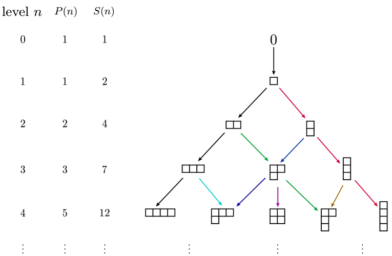
Figure 1: Young lattice.

Recall that the number of Young tableaux at level $n$ (i.e. with $n$ boxes) equals $P(n)$ (the partition number of $n$), while the number of edges at level $n$ (i.e. edges from level $n$ to level $n+1$) is $S(n)$ defined by

$$S(n)=\sum_{k=0}^{n}P(k)\ .$$ (5.16)

Their generating functions are

$$\sum^{\infty}_{n=0}P(n)\,x^{n}=\prod^{\infty}_{m=1}\frac{1}{1-x^{m}}\qquad\qquad\sum^{\infty}_{n=0}S(n)\,x^{n}=\frac{1}{1-x}\prod^{\infty}_{m=1}\frac{1}{1-x^{m}}\ .$$ (5.17)

$S(n)$ counts the number of scalar-like fields for which $\Lambda_{-}$ has $n$ boxes, and it grows exponentially with $n$. Therefore there are infinitely many such fields in the ’t Hooft limit, and we need to deal with an infinitely-degenerate operator mixing problem. However, as we shall see below in Section 5.3, the perturbation analysis has a lot of structure, and we can therefore understand at least its qualitative features in some detail.

5.2 The mixing matrix

Next we want to determine the mixing matrix $M$ explicitly. Its off-diagonal entries can be computed from the integral

$$\int d^{2}w\,\langle{\cal O}_{i}(z_{1},\bar{z}_{1}){\cal O}_{j}(z_{2},\bar{z}_{2})P(w,\bar{w})\rangle=\mathbf{P}_{ij}\frac{1}{|z_{1}-z_{2}|^{4h}}\ln{|z_{1}-z_{2}|}\ ,$$ (5.18)

where $h=\frac{1}{2}(1+\lambda)$ is the conformal dimension at $\mathcal{O}(g^{0})$. As explained above, the correlators in the integrand are first to be evaluated at finite $N$ and $k$, with $P=\Phi+\Phi^{*}$ as given in (5.3); the large $N$, $k$ limit is then only taken at the end. At finite $N$ and $k$ and up to ${\cal O}(\frac{1}{N})$, the three-point function of ${\cal O}_{1}$ and ${\cal O}_{2}$ with $\omega$ equals

$$\langle{\cal O}_{1}(z_{1},\bar{z}_{1}){\cal O}_{2}(z_{2},\bar{z}_{2})\,\omega(w,\bar{w})\rangle=C_{{\cal O}_{1}{\cal O}_{2}\,\omega}\left|\frac{1}{(z_{1}-z_{2})^{2h+\frac{1}{N}\Delta_{1}}(z_{2}-w)^{\frac{1}{N}\Delta_{2}}(z_{1}-w)^{\frac{1}{N}\Delta_{3}}}\right|^{2}\ ,$$ (5.19)

where $\Delta_{i}=\delta_{i}+\delta_{i+1}-\delta_{i+2}$, and $\delta_{i}$ (with $i\equiv i+3$) are the $\mathcal{O}(\frac{1}{N})$ corrections to the conformal dimensions

$${\cal O}_{1}:\ \ h_{1}=h+\frac{\delta_{1}}{N}\quad\qquad{\cal O}_{2}:\ \ h_{2}=h+\frac{\delta_{2}}{N}\quad\qquad\omega:\ \ h_{3}=\frac{\delta_{3}}{N}=\frac{\lambda^{2}}{2N}\ .$$ (5.20)

In order to deduce from this the correlator corresponding to $\Phi$, we then apply $\frac{1}{2h_{\omega}}\bar{L}_{-1}L_{-1}$ to (5.19) and obtain

$$\langle{\cal O}_{1}(z_{1},\bar{z}_{1}){\cal O}_{2}(z_{2},\bar{z_{2}})\,\Phi(w,\bar{w})\rangle\\ =\frac{4}{N\lambda^{2}}C_{{\cal O}_{1}{\cal O}_{2}\,\omega}\left|\frac{\frac{\Delta_{2}}{z_{2}-w}+\frac{\Delta_{3}}{z_{1}-w}}{(z_{1}-z_{2})^{2h+\frac{1}{N}\Delta_{1}}(z_{2}-w)^{\frac{1}{N}\Delta_{2}}(z_{1}-w)^{\frac{1}{N}\Delta_{3}}}\right|^{2}\ .$$ (5.21)

Finally, we take the large $N$ limit and evaluate the $w$-integral to obtain

$$\int d^{2}w\,\langle{\cal O}_{1}(z_{1},\bar{z}_{1}){\cal O}_{2}(z_{2},\bar{z}_{2})\,\Phi(w,\bar{w})\rangle=\Bigl{(}-\frac{16\pi}{N}\cdot\frac{\Delta_{2}\Delta_{3}}{\lambda^{2}}\cdot C_{{\cal O}_{1}{\cal O}_{2}\,\omega}\Bigr{)}\frac{1}{|z_{1}-z_{2}|^{4h}}\ln|z_{1}-z_{2}|\ ,$$ (5.22)

where $\Delta_{2}\Delta_{3}=(\frac{\lambda^{2}}{2})^{2}-(\delta_{1}-\delta_{2})^{2}$; here we have used the identity

$$\int d^{2}w\frac{1}{(w-z_{1})(\bar{w}-\bar{z}_{2})}=2\pi\ln r\,\Bigr{|}^{\infty}_{|z_{1}-z_{2}|}\ .$$ (5.23)

and dropped the $\ln\infty$ term.

Thus the $\mathbf{P}_{ij}$ entry in the mixing matrix between ${\cal O}_{i}$ and ${\cal O}_{j}$ is

$$\mathbf{P}_{ij}=\frac{16\pi}{N}\cdot C_{{\cal O}_{i}{\cal O}_{j}\,\omega}\cdot\Bigl{(}\frac{(\delta_{i}-\delta_{j})^{2}}{\lambda^{2}}-\frac{\lambda^{2}}{4}\Bigr{)}\ .$$ (5.24)

The coefficients $\delta_{i}$ and $\delta_{j}$ are read off from (5.14), and for the calculation of the structure constants $C_{{\cal O}_{i}{\cal O}_{j}\,\omega}$ we can use the results of [41, 42], see also [43] for earlier work. In particular, some of them were calculated explicitly in [41] using the Coulomb gas approach. Based on the large $N$ factorisation properties of these structure constants, [42] wrote down an effective Hamiltonian that captures the exact spectrum and cubic interactions in the ’t Hooft limit. Since we only need the large $N$ result, we can therefore directly use this effective Hamiltonian point of view.

We have worked out the explicit coefficients for the low-lying representations up to level $4$; some of the details are spelled out in Appendix C.

5.3 The eigenvalue problem

As we have reviewed above, the eigenvalues of the mixing matrix $M$ (5.9) give the perturbed conformal dimensions of the states under consideration. Thus we need to study the eigenproblem

$$M\cdot\vec{F}=\rho\,\vec{F}\ .$$ (5.25)

In the strict $N\rightarrow\infty$ limit $\vec{F}$ is an infinite-dimensional vector, and hence we expect $\rho$ to take a continuum of eigenvalues. Nevertheless, as we shall now explain, the structure of the eigenvalues can be identified naturally with that of the conformal dimensions of the scalar-like states in the ’t Hooft limit.

To start with we observe that the matrix $M$ has the form of a block Jacobi matrix

$$M(\{A_{n}\},\{B_{n}\})=\begin{pmatrix}A_{1}&B_{1}&0&0&0&\ldots\\ B^{T}_{1}&A_{2}&B_{2}&0&0&\ldots\\ 0&B^{T}_{2}&A_{3}&B_{3}&0&\ldots\\ 0&0&\ddots&\ddots&\ddots&0\end{pmatrix}$$ (5.26)

with

$$A_{n}=-4h\,\mathbf{1}_{S(n-1)\times S(n-1)}\ ,\qquad B_{n}=S(n-1)\times S(n)\,\textrm{matrix of rank $S(n-1)$ .}$$ (5.27)

The first few explicit expressions for $B_{n}$ are given in Appendix C. At low levels (for which we have worked them out, i.e. up to level $4$), the matrix $B_{n}$ has rank $S(n-1)$ provided that $\lambda\neq 0$. This is also what one should expect generically, and we therefore conjecture that this will continue to be true for all $n$.

Under this assumption the eigenvector problem (5.25) can be solved recursively, generalising the method of finding the eigenvalues of a scalar Jacobi matrix (which we review in Appendix D). We first decompose the eigenvector $\vec{F}$ into $\vec{F}=\{\vec{f}_{1},\vec{f}_{2},\ldots\}$, with $\vec{f}_{n}$ being a vector of dimension $S(n-1)$. Then for any given eigenvalue $\rho$, we have to solve the recursive relations

$$B_{n}\cdot\vec{f}_{n+1}=(\rho+4h)\vec{f}_{n}-B^{T}_{n-1}\cdot\vec{f}_{n-1}\ ,\qquad n\in\mathbb{N}_{\geq 1}\ ,$$ (5.28)

where we have set $\vec{f}_{0}\equiv 0$. Unlike the scalar Jacobi case for which the equation, at each level, is a scalar equation, now the equation at level $n$ is a matrix equation with $S(n-1)$ components for the $S(n)$ unknowns in $\vec{f}_{n+1}$. However, since $B_{n}$ has rank $S(n-1)$, we can always find a solution for $\vec{f}_{n+1}$, and hence an eigenvector with eigenvalue $\rho$. This solution is, however, not unique — in fact the kernel of $B_{n}$ has dimension $S(n)-S(n-1)=P(n)$, and thus, at every level $n$, we obtain $P(n)$ new families of solutions with $\vec{f}_{n+1}\neq 0$ but $\vec{f}_{i}=0$ for $i\leq n$.

In order to illustrate the structure of these various solutions let us describe some simple examples. Consider first the eigenvector that involves the original scalar representation $(\tiny\yng(1);0)$, i.e. the eigenvector with $f_{1}=1$. In this case, (5.28) is to be solved with the initial condition

$$f_{1}=1\ .$$ (5.29)

We may choose to supplement the recursion relation (5.28) with the requirement that $\vec{f}_{n+1}$ is orthogonal to the kernel of $B_{n}$,

$$\vec{f}_{n+1}^{\ T}\cdot g_{n}=0\qquad\forall g_{n}\in{\rm ker}(B_{n})$$ (5.30)

in order to guarantee that at level $n$ the corresponding eigenvector is orthogonal to the new families of eigenvectors that will appear at that level. These $P(n)$ equations, together with the $S(n-1)$ equations from (5.28), then uniquely determine the $S(n)$ components of $\vec{f}_{n+1}$ for all $n\geq 1$. This construction works for arbitrary $\rho$, and thus we conclude that the eigenvalue spectrum is continuous. This is consistent with the fact that, in the strict $N\rightarrow\infty$ limit, there are infinitely many states that are ‘mixed’ with $(\tiny\yng(1);0)$ via $P$.

In constructing the solution with $f_{1}=1$ we have in effect identified from the infinite mixing matrix $M$ (5.9) a sub-matrix (which is also infinite) that describes the mixing of $(\tiny\yng(1);0)$ with all states that couple to it at $\mathcal{O}(g)$. For example, the condition (5.30) with $n=1$ identifies a specific linear combination $\vec{f}^{\;(1)}_{2}$ of the two states $(\tiny\yng(2);\tiny\yng(1))$ and $(\tiny\yng(1,1);\tiny\yng(1))$ at level $2$, namely the linear combination that mixes with $(\tiny\yng(1);0)$ at order $g$, and similarly at the higher levels. However, since there are two scalar-like states at level $2$, we may construct a second state $\vec{f}^{\;(2)}_{2}$ from $(\tiny\yng(2);\tiny\yng(1))$ and $(\tiny\yng(1,1);\tiny\yng(1))$ that is orthogonal to $\vec{f}^{\;(1)}_{2}$ and hence lies in the kernel of $B_{1}$. It will generate a new family of solutions; this is to say, we can repeat the above procedure replacing $(\tiny\yng(1);0)$ by $\vec{f}^{\;(2)}_{2}$, i.e.  by imposing the initial conditions

$$f_{1}=0\ ,\qquad\vec{f}_{2}=\vec{f}^{\;(2)}_{2}\ .$$ (5.31)

The eigenvectors of this second sub-matrix then involve the states that mix with the linear combination of $(\tiny\yng(2);\tiny\yng(1))$ and $(\tiny\yng(1,1);\tiny\yng(1))$ given by $\vec{f}^{\;(2)}_{2}$ at order $g$. Again, we can find the solution for the $\vec{f}_{n}$ recursively, requiring as before (5.30) for $n\geq 2$, and since this can be done for any choice of $\rho$, it will also lead to a continuum of eigenvalues.

It should now be clear how to proceed in general: at level $n$, we find $P(n)=S(n)-S(n-1)$ new families of solutions for which $\vec{f}_{n+1}\neq 0$ lies in the kernel of $B_{n}$ and $\vec{f}_{j}=0$ for $j\leq n$. For each choice of $\vec{f}_{n+1}$ we can then construct an eigenvector recursively for any value of $\rho$. Thus each of these families will also give rise to a continuum of eigenvalues in the ’t Hooft limit. Altogether we therefore get at each level $n$, $P(n)$ families of eigenvectors, where each family has in turn a continuum of eigenvalues.

So far we have studied the eigenvalue problem in the strict $N\rightarrow\infty$ limit. It is natural to ask whether it is possible to formulate (and hopefully answer) the same question at large but finite $N$. At finite $(N,k)$, the number of scalar-like states is finite ($\sim\min(N,k)$) and correspondingly the spectrum is no longer a continuum. In fact, as is explained in Appendix D, it is straightforward to determine the eigenvalues of the finite problem by similar techniques. The resulting eigenvalues are then distributed symmetrically with respect to $h=\frac{1+\lambda}{2}$.

5.4 The CFT interpretation

As we have explained above, see eq. (5.9), each eigenstate with eigenvalue $\rho$ corresponds to a state in the spectrum with conformal dimension

$$h_{\rho}=-\frac{\rho}{4}=h-\frac{1}{4}(\rho+4h)\ ,\qquad\hbox{i.e.}\quad\delta h=-\frac{1}{4}(\rho+4h)\ .$$ (5.32)

We now want to match $\delta h$ as computed from the perturbative analysis, to the change in conformal dimension of the primary operators of the ${\cal W}_{N,k}$ models in the ’t Hooft limit as we vary $(N,k)$. Recall that the ’t Hooft parameter and the central charge of the ${\cal W}_{N,k}$ models are given by $\lambda$ and $c_{N,k}$ in (4.4) and (4.5), respectively. As we modify $N\mapsto N+\delta N$ and $k\mapsto k+\delta k$, they change to first order (in the ’t Hooft limit) as

$$\delta\lambda=-\frac{1}{N}\lambda(\lambda-1)\delta N-\frac{1}{N}\lambda^{2}\delta k$$ (5.33)

and

$$\delta c=(2\lambda+1)(\lambda-1)^{2}\delta N+2\lambda^{3}\delta k\ .$$ (5.34)

Furthermore, the $\gamma^{2}$ parameter, defined in (2.30), can be expressed in terms of $N$ and $k$ as

$$\gamma^{2}=\frac{64(k+1)(N-3)(N+1)(k+2N)(3k+2N)(3k+4N+3)}{(N-2)(2k+N)(2k+3N+2)\bigl{(}k(5N+17)(k+2N+1)+22N(N+1)\bigr{)}}\ ,$$ (5.35)

and thus it changes as

$$\delta\gamma^{2}=-\frac{128\lambda^{2}(\lambda-1)}{N(\lambda-2)^{2}(\lambda+2)^{2}}\,\delta N-\frac{128\lambda^{3}}{N(\lambda-2)^{2}(\lambda+2)^{2}}\,\delta k\ .$$ (5.36)

Given our general argument above (see the beginning of Section 5.1) we should expect that to first order $\delta\gamma^{2}=0$. Thus we conclude that $\delta k$ and $\delta N$ should be related as

$$\delta k=-\frac{(\lambda-1)}{\lambda}\,\delta N\ .$$ (5.37)

Note that then we also have $\delta\lambda=0$, and

$$\delta c=(1-\lambda^{2})\,\delta N\ .$$ (5.38)

Under this deformation the conformal dimensions of the scalar-like representations in eq. (5.14) change as

$$\delta h(\Lambda_{+};\Lambda_{-})=-\frac{1}{2}\,\frac{\delta N}{N}\,\Bigl{[}\frac{\lambda^{2}B_{-}-1}{N}+\frac{(D_{+}-D_{-})}{N}\,\lambda\Bigr{]}\ .$$ (5.39)

This should now be compared to (5.32) above.

In order to do so, let us first explain how the structure of the answer is the same on both sides. As we have seen above, the eigenstates of the mixing matrix $M$ organise themselves into families, where at each level $n$, $P(n)$ new families of eigenvectors of $M$ emerge. Each such family gives rise to a continuum of eigenvalues $\rho$.

From the viewpoint of the minimal model representations on the other hand, let us consider the ‘branches’ of the Young lattice. Recall that the edges of the Young lattice are in one-to-one corresponding to the scalar-like states $(\Lambda_{+};\Lambda_{-})$. A branch is a collection of edges, starting from a given level and including one edge at each subsequent level. Given the structure of the Young lattice, see in particular eq. (5.16), it is clear that at each level $n$, there are $P(n)$ edges that are not on any branch that emerges before level $n$ and are the roots of $P(n)$ new branches. Thus the branches of the Young lattice are in natural one-to-one correspondence to the families of eigenstates of $M$.

One definite (and natural) way to construct these branches is as follows. Let us begin with the original scalar representation $(\tiny\yng(1);0)$, and define its branch by picking one representation at each level (i.e. for each value of $B_{-}$), namely the one for which $\Delta D\equiv D_{+}-D_{-}$ is maximal. (This is the branch described by the black edges in Fig. 1.) Then we consider the corresponding transposed branch, where we replace each representation $(\Lambda_{+};\Lambda_{-})$ by its transpose $(\Lambda_{+}^{t};\Lambda_{-}^{t})$. Obviously the transposed branch shares the representation $(\tiny\yng(1);0)$ with the original branch; thus we should take it to start from $(\tiny\yng(1,1);0)$ instead — this then leads to the branch corresponding to the red edges in Fig. 1. Note that taking the transpose does not modify $B_{-}$ — so the transposed branch also has one representation at each level — but it changes the sign of both $D_{+}$ and $D_{-}$, and hence the sign of $\Delta D$. Thus the change in conformal dimensions of the transposed representations are, apart from the ‘drift term’ $(\lambda^{2}B_{-}-1)/N$, opposite to those of the original representations, see eq. (5.39).

We now propose that these two branches together are to be mapped to the first two families that come out of the perturbative analysis, i.e. the family (5.29) that mixes with $(\tiny\yng(1);0)$, and the family (5.31) that mixes with the level $2$ state given by $\vec{f}^{\;(2)}_{2}$. In particular, in the ’t Hooft limit the ratio $\Delta D/N$ (as well as the drift term $(\lambda^{2}B_{-}-1)/N$) become continuous variables, and hence the branches of minimal model representations lead to a continuum of perturbed conformal dimensions; this matches the continuum for $\rho$ we found above. At finite $N$ and $k$, the two branches contain the same number of states as the two families, and their eigenvalues are, except for the ‘drift term’ $(\lambda^{2}B_{-}-1)/N$, symmetrically distributed around $h$, thereby matching the structure found in the perturbative analysis. (We shall comment below on the origin of the ‘drift term’ in the perturbative analysis.)

It should now be clear how to continue. While the above two branches account for all representations up to level $2$, there are two more branches starting with edges linking level $2$ to level $3$. Again, they can be completed into branches by picking at each level a representation with the second biggest (or smallest) value for $\Delta D$ — these two branches can be chosen to be transposes of one another, and they correspond to the solutions of the perturbative analysis with $f_{1}=\vec{f}_{2}=0$ and $\vec{f}_{3}\neq 0$. (They are described by the blue and green edges in Fig. 1.) Furthermore, their eigenvalues will, again apart from the drift term, be symmetrically distributed around $h$.

Continuing in this manner, there will be $P(n)$ branches emerging at level $n$, and their conformal weights will, apart from the drift term, be symmetrically distributed around $h$. This matches nicely the structure of the eigenvalues as computed in the perturbative analysis.

It remains to comment on the reason that the ‘drift term’ $(\lambda^{2}B_{-}-1)/N$ in (5.39) is invisible to the perturbation analysis of the previous subsection. Recall that in the formula of the quadratic Casimir (5.11), the term proportional to $B$ is the leading term in the $\frac{1}{N}$ expansion. It should therefore be considered as the ‘classical’ contribution, while the term proportional to $D$ corresponds to the first $\frac{1}{N}$ correction. Correspondingly, in the expansion of the conformal dimension (5.14), although both $\frac{\lambda^{2}B_{-}-1}{2N}$ and $\frac{D_{+}-D_{-}}{2N}\,\lambda$ are of $\mathcal{O}(\frac{1}{N})$, in some sense only the first one is ‘classical’. Therefore in the large but finite $N$ case, we shouldn’t merely truncate the infinite mixing matrix to a finite one; we should also shift the diagonal entries of the mixing matrix by the ‘classical’ piece $(-4)\frac{\lambda^{2}B_{-}-1}{2N}$. Once this is done, the new eigenvalues are distributed symmetrically with respect to the shifted $\mathcal{O}(g^{0})$ conformal dimension, thus explaining the ‘drift term’ $\frac{\lambda^{2}B_{-}-1}{N}$ in (5.39).

We therefore regard this as good evidence for the assertion that the perturbation by $P$ corresponds to switching on the above $\frac{1}{N}$ corrections of the ${\cal W}_{N,k}$ minimal models in the ’t Hooft limit. We should also mention that this identification fits with what we have seen explicitly for the special cases $\lambda=0$ and $\lambda=1$ above. Indeed, for $\lambda=1$, it follows from (5.36) that in order for $\delta\gamma^{2}=0$, we need to take $\delta k=0$, see also (5.37). But then, it follows from (5.33) and (5.34) that both $\delta\lambda=\delta c=0$, i.e. that the perturbation does not change anything, in nice agreement with what we saw in Section 4.4. From the point of view of the perturbative analysis, at $\lambda=1$ where $N\rightarrow\infty$ at finite $k$, it is no longer appropriate to make a $\frac{1}{N}$ expansion, but we should rather perform a $\frac{1}{k}$ expansion, replacing $\frac{1}{N}$ by $\frac{1}{k}$ as in (5.15). But then (5.24) vanishes at $\lambda=1$, i.e. the spectrum is not perturbed at all.

On the other hand, for $\lambda=0$, $\delta\lambda=0$ automatically from (5.33) and $\delta c=\delta N$ from (5.34). In this case the condition $\delta\gamma^{2}=0$ from (5.36) does not impose any restriction on $\delta k$ and $\delta N$, and thus $\delta c=\delta N$ will be non-zero. Note, however, that the coefficient of the $\Delta D$-term in (5.39) vanishes for $\lambda=0$. This is reflected, in the context of the perturbation computation, by the fact that the analysis breaks down for $\lambda=0$ as the $B_{n}$ do not have maximal rank any longer. (For instance, the rank of $B_{3}$ is ${\rm rk}(B_{3})=3<4$, at $\lambda=0$.) This reduction in the rank of $B_{n}$ at $\lambda=0$ is a sign that the scalar-like states do not ‘mix’ strongly enough to break the degeneracy of their conformal dimensions.

6 Conclusions

In this paper we have studied the behaviour of the ${\cal W}_{\infty}[\lambda]$ theories under perturbations that preserve the symmetry algebra to first order. In particular, we have found that the minimal models possess such a perturbing field in the ’t Hooft limit, and we have shown that it corresponds to switching on the $\frac{1}{N}$ corrections, while keeping $\lambda$ fixed at first order. Since the theory at finite $N$ involves necessarily the light states (that may be taken to decouple in the ’t Hooft limit [22]), it is not surprising that these states, as well as their descendants, play an important part in the analysis. The perturbative analysis is technically rather demanding since the strict ’t Hooft limit is a degenerate point where infinitely many states — the analogues of the light states at $h=\frac{1}{2}(1+\lambda)$ — have the same conformal dimension and hence can mix in perturbation theory. However, as we have seen, the structure of the theory is sufficiently rigid so as to allow one to understand at least some of the qualitative features.

We should mention that the 2d case we have considered here differs qualitatively from what happens in higher dimensions. In particular, it was shown in [10, 11] that for $d\geq 3$, the $\frac{1}{N}$ corrections necessarily break the higher spin symmetry to first order. This is to be contrasted with what we have found here, namely that there are perturbing fields that preserve the symmetry at least to first order.

Perturbations of these ${\cal W}_{\infty}[\lambda]$ algebras, not necessarily preserving the higher spin symmetry, will also be important in order to connect suitable generalisations of these theories to string theory. In particular, it would be interesting to understand what the effect of the exactly marginal perturbing field of the large ${\cal N}=4$ higher spin theory of [44] is. It should be possible to study this question with similar techniques as those used in the present paper.

Appendix A The free fermion theory at $\lambda=0$

In this appendix we collect some of the OPEs we have calculated for the free fermion theory. Using Wick’s theorem it is not difficult to work out the singular part of the OPEs of these currents. In particular, we find that

$$J(z_{1})\,J(z_{2}) \sim \frac{N}{(z_{1}-z_{2})^{2}}$$ (A.1)

$$T(z_{1})\,T(z_{2}) \sim \frac{N/2}{(z_{1}-z_{2})^{4}}+\frac{2\,T(z_{2})}{(z_{1}-z_{2})^{2}}+\frac{T^{\prime}(z_{2})}{(z_{1}-z_{2})}$$ (A.2)

$$T(z_{1})\,J(z_{2}) \sim \frac{J(z_{2})}{(z_{1}-z_{2})^{2}}+\frac{J^{\prime}(z_{2})}{(z_{1}-z_{2})}$$ (A.3)

$$J(z_{1})\,T(z_{2}) \sim \frac{J(z_{2})}{(z_{1}-z_{2})^{2}}\ ,$$ (A.4)

$$J(z_{1})W(z_{2}) \sim \frac{2}{(z_{1}-z_{2})^{2}}\,T(z_{2})$$ (A.5)

$$T(z_{1})W(z_{2}) \sim \frac{1}{(z_{1}-z_{2})^{4}}\,J(z_{2})+\frac{3}{(z_{1}-z_{2})^{2}}W(z_{2})+\frac{1}{(z_{1}-z_{2})}W^{\prime}(z_{2})\ ,$$ (A.6)

$$W(z_{1})W(z_{2}) \sim \frac{2N/3}{(z_{1}-z_{2})^{6}}+\frac{4T(z_{2})}{(z_{1}-z_{2})^{4}}+\frac{2T^{\prime}(z_{2})}{(z_{1}-z_{2})^{3}}+\frac{4U(z_{2})+\frac{3}{5}T^{\prime\prime}(z_{2})}{(z_{1}-z_{2})^{2}}$$ (A.7)

$$\ +\frac{2U^{\prime}(z_{2})+\frac{2}{15}T^{\prime\prime\prime}(z_{2})}{(z_{1}-z_{2})}\ ,$$

where $\sim$ always denotes the singular part of the operator product expansion.

Appendix B The free boson theory at $\lambda=1$

The first few OPEs of the free boson higher spin fields defined in eq. (3.1) are explicitly given by ($z_{12}\equiv z_{1}-z_{2}$)

$$T(z_{1})W^{3}(z_{2}) \sim \frac{3}{z_{12}^{2}}W^{3}(z_{2})+\frac{1}{z_{12}}\partial W^{3}(z_{2})$$ (B.1)

$$T(z_{1})W^{4}(z_{2}) \sim \frac{192}{5}\frac{T(z_{2})}{z_{12}^{4}}+\frac{4}{z_{12}^{2}}W^{4}(z_{2})+\frac{1}{z_{12}}\partial W^{4}(z_{2})$$ (B.2)

$$W^{3}(z_{1})W^{3}(z_{2}) \sim 48\left[\frac{T}{z_{12}^{4}}+\frac{1}{2}\frac{\partial T}{z_{12}^{3}}+\frac{3}{20}\frac{\partial^{2}T}{z_{12}^{2}}+\frac{1}{30}\frac{\partial^{3}T}{z_{12}}\right]$$ (B.3)

$$+\frac{4}{z_{12}^{2}}W^{4}(z_{2})+\frac{2}{z_{12}}\partial W^{4}(z_{2})+16\frac{k}{z_{12}^{6}}$$

$$W^{3}(z_{1})W^{4}(z_{2}) \sim \frac{768}{5}\left[\frac{W^{3}}{z_{12}^{4}}+\frac{1}{3}\frac{\partial W^{3}}{z_{12}^{3}}+\frac{1}{14}\frac{\partial^{2}W^{3}}{z_{12}^{2}}+\frac{1}{84}\frac{\partial^{3}W^{3}}{z_{12}}\right]$$ (B.4)

$$+\frac{5}{z_{12}^{2}}W^{5}(z_{2})+\frac{2}{z_{12}}\partial W^{5}(z_{2})$$

$$W^{4}(z_{1})W^{4}(z_{2}) \sim \frac{12288}{5}\left[\frac{T}{z_{12}^{6}}+\frac{1}{2}\frac{\partial T}{z_{12}^{5}}+\frac{3}{20}\frac{\partial^{2}T}{z_{12}^{4}}+\frac{1}{30}\frac{\partial^{3}T}{z_{12}^{3}}+\frac{1}{168}\frac{\partial^{4}T}{z_{12}^{2}}+\frac{1}{1120}\frac{\partial^{5}T}{z_{12}}\right]$$ (B.5)

$$+\frac{1728}{5}\left[\frac{W^{4}}{z_{12}^{4}}+\frac{1}{2}\frac{\partial W^{4}}{z_{12}^{3}}+\frac{5}{36}\frac{\partial^{2}W^{4}}{z_{12}^{2}}+\frac{1}{36}\frac{\partial^{3}W^{4}}{z_{12}}\right]$$

$$+\frac{6}{z_{12}^{2}}W^{6}(z_{2})+\frac{3}{z_{12}}\partial W^{6}(z_{2})+\frac{3072}{5}\frac{k}{z_{12}^{8}}\ .$$

Appendix C Explicit mixing matrices

Using the notation of (5.26), the first few explicit expressions for the $B_{n}$ are as follows

• $\frac{N}{16\pi g}\,B_{1}\,:$

  	$(\tiny\yng(1,1);\tiny\yng(1))$	$(\tiny\yng(2);\tiny\yng(1))$
  $(\tiny\yng(1);0)$	$\frac{1-\lambda}{\sqrt{2}}$	$\frac{1+\lambda}{\sqrt{2}}$

• $\frac{N}{16\pi g}\,B_{2}\,:$

  	$(\tiny\yng(1,1,1);\tiny\yng(1,1))$	$(\tiny\yng(2,1);\tiny\yng(2))$	$(\tiny\yng(2,1);\tiny\yng(1,1))$	$(\tiny\yng(3);\tiny\yng(2))$
  $(\tiny\yng(1,1);\tiny\yng(1))$	$\sqrt{\frac{2}{3}}(1-\lambda)$	0	$\frac{2+\lambda}{\sqrt{3}}$	0
  $(\tiny\yng(2);\tiny\yng(1))$	0	$\frac{2-\lambda}{\sqrt{3}}$	0	$\sqrt{\frac{2}{3}}(1+\lambda)$

• $\frac{N}{16\pi g}\,B_{3}\,:$

  	$(\tiny\yng(2,2);\tiny\yng(2,1))$	$(\tiny\yng(2,1,1);\tiny\yng(2,1))$	$(\tiny\yng(3,1);\tiny\yng(2,1))$	$(\tiny\yng(1,1,1,1);\tiny\yng(1,1,1))$	$(\tiny\yng(2,1,1);\tiny\yng(1,1,1))$	$(\tiny\yng(3,1);\tiny\yng(3))$	$(\tiny\yng(4);\tiny\yng(3))$
  $(\tiny\yng(1,1,1);\tiny\yng(1,1))$	$0$	$0$	$0$	$\frac{\sqrt{3}(-1+\lambda)}{2}$	$-\frac{3+\lambda}{2}$	0	0
  $(\tiny\yng(2,1);\tiny\yng(2))$	$\frac{\sqrt{3}(1-\lambda)}{2\sqrt{2}}$	$\frac{3-\lambda}{4}$	$\frac{3(1+\lambda)}{4}$	0	0	0	0
  $(\tiny\yng(2,1);\tiny\yng(1,1))$	$-\frac{\sqrt{3}(1+\lambda)}{2\sqrt{2}}$	$\frac{3(-1+\lambda)}{4}$	$-\frac{3+\lambda}{4}$	0	0	0	0
  $(\tiny\yng(3);\tiny\yng(2))$	0	0	0	0	0	$\frac{3-\lambda}{2}$	$\frac{\sqrt{3}(1+\lambda)}{2}$

Appendix D The eigenproblem of a scalar Jacobi matrix

Let us consider the perturbative solution corresponding to $f_{1}=1$, i.e. the solution that involves the original scalar field ${\cal O}\equiv(\tiny\yng(1),0)$ itself. As was argued in section 5.3, the perturbative analysis will mix to this state one specific linear combination of scalar-like states at each level; thus we can consider the truncated problem, where instead of the full matrix $M$ we just consider the eigenvalue problem

$$J\cdot\vec{F}=\rho\,\vec{F}\qquad\qquad\textrm{with}\quad\vec{F}=(f_{1},f_{2},\ldots)$$ (D.1)

for the ‘scalar Jacobi matrix’

$$J(\{a_{n}\},\{b_{n}\})=\begin{bmatrix}a_{1}&b_{1}&0&0&0&\ldots\\ b_{1}&a_{2}&b_{2}&0&0&\ldots\\ 0&b_{2}&a_{3}&b_{3}&0&\ldots\\ 0&0&\ddots&\ddots&\ddots&\end{bmatrix}\ ,$$ (D.2)

where now all $a_{n}$ and $b_{n}$ are numbers. This can be solved recursively; since the value of $f_{1}$ only affects the overall normalisation, we can start by setting $f_{1}=1$. Then given any $\rho\in\mathbb{C}$, we solve for $f_{n}(\rho)$ as

$$f_{1}=1$$

$$a_{1}f_{1}+b_{1}f_{2}=\rho\,f_{1} \rightarrow f_{2}=\frac{1}{b_{1}}(\rho-a_{1})f_{1}$$ (D.3)

$$\dots$$

$$b_{n-1}f_{n-1}+a_{n}f_{n}+b_{n}f_{n+1}=\rho\,f_{n} \rightarrow f_{n+1}=\frac{1}{b_{n}}\bigl{[}(\rho-a_{n})f_{n}-b_{n-1}f_{n-1}\bigr{]}$$

$$\dots$$

Note that, by construction, $f_{n}(\rho)$ is a polynomial of degree $n-1$ in $\rho$. If the Jacobi matrix is strictly infinite, this is the most general solution.

If the Jacobi matrix truncates to some finite matrix, say to a matrix of size $K\times K$ — this will be the case for finite $N$ and $k$ — then the analysis can be performed similarly. We simply extend the Jacobi matrix to an infinite matrix by choosing the $a_{n}$ and $b_{n}$ for $n>K$ arbitrarily. Then we can construct recursive eigenvalues as above. Up to level $K$ the solution agrees with the solution to the actual eigenvalue problem we are interested in, so all we have to require is that the analysis terminates at level $K$, i.e. that $f_{K+1}(\rho)=0$. Since $f_{n}(\rho)$ is a polynomial of degree $n-1$ in $\rho$, this gives rise to $K$ different solutions, as expected. Note that if all $a_{i}$, $i=1,\ldots,K$ agree, $a_{i}\equiv a$, then $f_{n}(\rho)$ is an even (odd) polynomial of $\rho-a$ if $n$ is odd (even); in this case the eigenvalues will be symmetrically distributed around $\rho=a$. If the diagonal entries exhibit some ‘drift’, we expect that also the eigenvalues will become symmetrically distributed w.r.t. some shifted mean.

References

• [1] I.R. Klebanov and A.M. Polyakov, “AdS dual of the critical O(N) vector model,” Phys. Lett. B 550, 213 (2002) [arXiv:hep-th/0210114].
• [2] B. Sundborg, ‘Stringy gravity, interacting tensionless strings and massless higher spins,” Nucl. Phys. Proc. Suppl.  102, 113 (2001) [arXiv:hep-th/0103247].
• [3] E. Witten, talk at the John Schwarz 60-th birthday symposium (Nov. 2001),
http://theory.caltech.edu/jhs60/witten/1.html.
• [4] A. Mikhailov, “Notes on higher spin symmetries,” arXiv:hep-th/0201019.
• [5] E. Sezgin and P. Sundell, “Massless higher spins and holography,” Nucl. Phys. B 644, 303 (2002) [Erratum-ibid. B 660, 403 (2003)] [arXiv:hep-th/0205131].
• [6] E. Sezgin and P. Sundell, “Holography in 4D (super) higher spin theories and a test via cubic scalar couplings,” JHEP 0507, 044 (2005) [arXiv:hep-th/0305040].
• [7] M.A. Vasiliev, “Consistent equation for interacting gauge fields of all spins in (3+1)-dimensions,” Phys. Lett. B 243, 378 (1990).
• [8] S. Giombi and X. Yin, “Higher spin gauge theory and holography: the three-point functions,” JHEP 1009, 115 (2010) [arXiv:0912.3462 [hep-th]].
• [9] S. Giombi and X. Yin, “Higher spins in AdS and twistorial holography,” JHEP 1104, 086 (2011) [arXiv:1004.3736 [hep-th]].
• [10] J. Maldacena and A. Zhiboedov, “Constraining conformal field theories with a higher spin symmetry,” J. Phys. A 46, 214011 (2013) [arXiv:1112.1016 [hep-th]].
• [11] J. Maldacena and A. Zhiboedov, “Constraining conformal field theories with a slightly broken higher spin symmetry,” Class. Quant. Grav. 30, 104003 (2013) [arXiv:1204.3882 [hep-th]].
• [12] O. Aharony, G. Gur-Ari and R. Yacoby, “d=3 bosonic vector models coupled to Chern-Simons gauge theories,” JHEP 1203, 037 (2012) [arXiv:1110.4382 [hep-th]].
• [13] S. Giombi, S. Minwalla, S. Prakash, S.P. Trivedi, S.R. Wadia and X. Yin, “Chern-Simons theory with vector fermion matter,” Eur. Phys. J. C 72, 2112 (2012) [arXiv:1110.4386 [hep-th]].
• [14] C.-M. Chang, S. Minwalla, T. Sharma and X. Yin, “ABJ triality: from higher spin fields to strings,” J. Phys. A 46, 214009 (2013) [arXiv:1207.4485 [hep-th]].
• [15] M.R. Gaberdiel and R. Gopakumar, “An AdS3 dual for minimal model CFTs,” Phys. Rev. D 83, 066007 (2011) [arXiv:1011.2986 [hep-th]].
• [16] S.F. Prokushkin and M.A. Vasiliev, “Higher spin gauge interactions for massive matter fields in 3d AdS space-time,” Nucl. Phys. B 545, 385 (1999) [arXiv:hep-th/9806236 [hep-th]].
• [17] S.F Prokushkin and M.A. Vasiliev, “3-d higher spin gauge theories with matter,”
arXiv:hep-th/9812242 [hep-th].
• [18] M. Henneaux and S.J. Rey, “Nonlinear W(infinity) algebra as asymptotic symmetry of three-dimensional higher spin Anti-de Sitter gravity,” JHEP 1012, 007 (2010) [arXiv:1008.4579 [hep-th]].
• [19] A. Campoleoni, S. Fredenhagen, S. Pfenninger and S. Theisen, “Asymptotic symmetries of three-dimensional gravity coupled to higher-spin fields,” JHEP 1011, 007 (2010) [arXiv:1008.4744 [hep-th]].
• [20] M.R. Gaberdiel and T. Hartman, “Symmetries of holographic minimal models,” JHEP 1105, 031 (2011) [arXiv:1101.2910 [hep-th]].
• [21] A. Campoleoni, S. Fredenhagen and S. Pfenninger, “Asymptotic W-symmetries in three-dimensional higher-spin gauge theories,” JHEP 1109, 113 (2011) [arXiv:1107.0290 [hep-th]].
• [22] M.R. Gaberdiel, R. Gopakumar, T. Hartman, and S. Raju, “Partition functions of holographic minimal models,” JHEP 1108, 077 (2011) [arXiv:1106.1897 [hep-th]].
• [23] M.R. Gaberdiel and R. Gopakumar, “Triality in minimal model holography,” JHEP 1207, 127 (2012) [arXiv:1205.2472 [hep-th]].
• [24] M.R. Gaberdiel and P. Suchanek, “Limits of minimal models and continuous orbifolds,” JHEP 1203, 014 (2012) [arXiv:1112.1708 [hep-th]].
• [25] E. Bergshoeff, M.P. Blencowe and K.S. Stelle, “Area preserving diffeomorphisms and higher spin algebra,” Commun. Math. Phys.  128, 213 (1990).
• [26] E. Bergshoeff, C.N. Pope, L.J. Romans, E. Sezgin and X. Shen, “The super W(infinity) algebra,” Phys. Lett. B 245, 447 (1990).
• [27] D.A. Depireux, “Fermionic realization of W(1+infinity),” Phys. Lett. B 252, 586 (1990).
• [28] M.R. Gaberdiel, T. Hartman and K. Jin, “Higher spin black holes from CFT,” JHEP 1204, 103 (2012) [arXiv:1203.0015 [hep-th]].
• [29] M. Kelm and C. Vollenweider, private communication.
• [30] P. Di Francesco, P. Mathieu and D. Sénéchal, “Conformal Field Theory,” Springer (1997).
• [31] S. Banerjee, S. Hellerman, J. Maltz and S.H. Shenker, “Light states in Chern-Simons theory coupled to fundamental matter,” JHEP 1303, 097 (2013) [arXiv:1207.4195 [hep-th]].
• [32] I. Bakas and E. Kiritsis, “Bosonic realisation of a universal W algebra and $\mathbb{Z}_{\infty}$ parafermions,” Nucl. Phys. B 343, 185 (1990) [Erratum ibid. B 350, 512 (1991)].
• [33] S. Fredenhagen, M.R. Gaberdiel and C.A. Keller, “Symmetries of perturbed conformal field theories,” J. Phys. A 40, 13685 (2007) [arXiv:0707.2511 [hep-th]].
• [34] J.L. Cardy, “Conformal invariance and statistical mechanics,” in: Les Houches XLIX (1988), Fields, Strings and Critical Phenomena, eds. E. Brezin and J. Zinn-Justin, North-Holland (1990).
• [35] S. Chaudhuri and J.A. Schwartz, “A criterion for integrably marginal operators,” Phys. Lett. B 219, 291 (1989).
• [36] C.-M. Chang and X. Yin, “A semi-local holographic minimal model,” arXiv:1302.4420 [hep-th].
• [37] J.L. Cardy, “Continuously varying exponents and the value of the central charge,” J. Phys. A 20, L891 (1987).
• [38] A.B. Zamolodchikov, “Integrals of motion in scaling three state Potts model field theory,” Int. J. Mod. Phys. A 3, 743 (1988).
• [39] A.B. Zamolodchikov, “Integrable field theory from conformal field theory,” in: Integrable Systems in Quantum Field Theory and Statistical Mechanics, Adv. Studies in Pure Mathematics 19, 641 (1989).
• [40] R.P. Stanley, “Enumerative combinatorics,” 2nd ed., Cambridge University Press (2012).
• [41] C.-M. Chang and X. Yin, “Correlators in $W_{N}$ minimal model revisited,” JHEP 1210, 050 (2012) [arXiv:1112.5459 [hep-th]].
• [42] A. Jevicki and J. Yoon, “Field theory of primaries in WN minimal models,”
arXiv:1302.3851 [hep-th].
• [43] K. Papadodimas and S. Raju, “Correlation functions in holographic minimal models,” Nucl. Phys.  B 856, 607 (2012) [arXiv:1108.3077 [hep-th]].
• [44] M.R. Gaberdiel and R. Gopakumar, “Large $\mathcal{N}=4$ holography,” arXiv:1305.4181 [hep-th].