fig[FIGURE][List of mytype]

Phase diagram of strongly interacting matter under strong magnetic fields

Pablo G. Allen¹ and Norberto N. Scoccola^1,2,3
1Department of Theoretical Physics, GIyA, CNEA, Libertador 8250, 1429.
²CONICET, Av. Rivadavia 1917, 1033.
³Universidad Favaloro, Solís 453, 1078, Buenos Aires, Argentina.

1 Introduction

The understanding of the behaviour of strongly interacting matter at finite temperature and density is of fundamental interest and has applications in cosmology, in the astrophysics of neutron stars and in the physics of relativistic heavy ion collisions. Given the possible existence of strong magnetic fields in the mentioned situations, their effect on the QCD phase diagram has recently become a topic of increasing interest[1]. Here, we report on the study of this issue in the framework of the two flavor Nambu-Jona-Lasinio model with Polyakov loop (PNJL) [2] and an extension of it, the so-called entangled PNJL model (EPNJL)[3]. Previous analyses at finite temperature can be found in Ref.[4].

2 Formalism

Our starting point for the study of quark matter is the PNJL model, which is constructed by incorporating the Polyakov Loop (PL) into the finite temperature and chemical potential Nambu-Jona-Lasinio (NJL) model[5]. Since the model under consideration is not renormalizable, we need to specify a regularization scheme. Here, we introduce a sharp cut-off in 3-momentum space, only for the divergent ultra-violet integrals. The Euclidean PNJL action coupled to the EM field reads

$$S_{E}=\int d^{4}x\left\{\overline{\psi}(-i\gamma^{\mu}D_{\mu}+m_{0})\psi-G\left[(\overline{\psi}\psi)^{2}+(\overline{\psi}i\tau\gamma_{5}\psi)^{2}\right]+{\cal U}(\Phi[{\cal G}(x)])\right\},$$ (1)

where $m_{0}$ is the current mass and G is a coupling constant. Together with the cut-off $\Lambda$, they completely determine the model. Two sets of parameters were used. For Set 1: $m_{0}=5.6$ MeV, $\Lambda=587.9$ MeV, $G\Lambda^{2}=2.44$, and for Set 2: $m_{0}=5.5$ MeV, $\Lambda=631.5$ MeV, $G\Lambda^{2}=2.19$. The coupling of the quarks to the (electro)magnetic field ${\cal A}_{\mu}$ and the gluon field ${\cal G}_{\mu}$ is implemented via the covariant derivative $D_{\mu}=\partial_{\mu}-iq_{f}{\cal A}_{\mu}-i{\cal G}_{\mu}$ where $q_{f}$ represents the quark electric charge ($q_{u}/2=-q_{d}=e/3$). We consider a static and constant magnetic field in the $z$ direction, ${\cal A}_{\mu}=\delta_{\mu 2}x_{1}B$. Concerning the gluon fields, we assume that quarks move on a constant background field ${\cal G}_{\mu}=\delta_{\mu 4}\phi$. Then the traced Polyakov loop, which in the infinite quark mass limit can be taken as an order parameter of confinement, is given by $\Phi=\frac{1}{3}{\rm Tr}\,\exp(i\phi/T)$. We work in the so-called Polyakov gauge, in which $\phi=\phi_{3}\lambda_{3}+\phi_{8}\lambda_{8}$. This leaves only two independent variables, $\phi_{3}$ and $\phi_{8}$. In the case of $\mu=0$ the traced Polyakov loop in the Mean Field Approximation (MFA) is expected to be a real quantity implying $\phi_{8}=0$, a condition that we assume to be valid also for finite real $\mu$. The MFA traced Polyakov loop reads then $\Phi=\Phi^{*}=\left[1+2\,\cos\left(\phi_{3}/T\right)\right]/3$. To proceed we need to specify the explicit form of the Polyakov loop effective potential ${\cal{U}}(\Phi,T)$. Here we consider [6]

$${\cal U}(\Phi,T)=-\frac{1}{2}a(T)\Phi\Phi^{*}+b(T)\ln[1-6\Phi\Phi^{*}+4(\Phi^{3}+\Phi^{*3})-3(\Phi\Phi^{*})^{2}],$$ (2)

where $a(T)=a_{0}+a_{1}\left(T_{0}/T\right)+a_{2}\left(T_{0}/T\right)^{2}$ and $b(T)=b_{3}\left(T_{0}/T\right)^{3}$. The values of the constants $a_{i},b_{3}$ can be fitted to pure gauge lattice QCD (LQCD) results, leading to $a_{0}=3.51\ ,a_{1}=-2.47\ ,a_{2}=15.2\ ,b_{3}=-1.75$ [6]. The scale parameter $T_{0}$ corresponds in principle to the deconfinement transition temperature in the pure Yang-Mills theory, $T_{0}=270$ MeV. However, it has been argued that in the presence of light dynamical quarks this temperature scale should be adequately reduced [7]. Thus, we also consider values $T_{0}\sim 200$ MeV in our calculations.

In the standard PNJL model the quark-quark coupling constant $G$ is independent of the PL. To account for further correlations between the quark and colour sector, a PL dependent $G(\Phi)$ can be introduced, leading to the EPNJL model. Namely,

$$G(\Phi)=\left[1-\alpha_{1}\Phi\Phi^{*}-\alpha_{2}(\Phi^{3}+\Phi^{*3})\right]G$$ (3)

The choice $\alpha_{1}=\alpha_{2}=0.2$ reproduces the LQCD phase diagram at imaginary $\mu$[3].

Finally, using the Matsubara formalism to account for finite $T$ and $\mu$ in the quark sector, the MFA thermodynamical potential for the models under consideration read

$$\Omega_{MFA}(M,\Phi) = \frac{(M-m_{0})^{2}}{4G(\Phi)}+{\cal U}(\Phi,T)-\frac{N_{c}N_{f}}{\pi^{2}}\int_{0}^{\Lambda}dp\ p^{2}\sqrt{p^{2}+M^{2}}$$ (4)

$$- \!\!\!\frac{N_{c}}{2\pi^{2}}\!\sum_{f=u,d}(q_{f}B)^{2}\left[\zeta^{\prime}(-1,x_{f})+\frac{x_{f}^{2}}{4}-\frac{1}{2}(x_{f}^{2}-x_{f})\log x_{f}\right]$$

$$- \!\!\!\frac{T}{2\pi}\!\sum_{s,k,c,f}\!\alpha_{k}|q_{f}|B\!\int\!\frac{dp_{z}}{2\pi}\ln\!\left[1+\exp\left(-\frac{E_{f}(p_{z},k)+s\ \mu+i\phi_{c}}{T}\right)\right]\!,$$

where $s=\pm 1$, $\alpha_{k}=2-\delta_{k0}$, $E_{f}(p_{z},k)=\sqrt{M^{2}+p_{z}^{2}+2k|q_{f}|B}$, and $\phi_{c}=\phi_{3},\phi_{3},-2\phi_{3}$ for $c=r,g,b$, respectively. In addition, $x_{f}=M^{2}/(2|q_{f}|B)$. The dressed quark mass $M$ and the PL are found as solution of the gap equations, $\partial\Omega_{MFA}/\partial M=\partial\Omega_{MFA}/\partial\Phi=0$. Once the solutions are found, chiral and deconfinement critical temperatures for crossover transitions are defined as the peaks of the corresponding susceptibilities $\chi_{ch}=\partial M/\partial T$ and $\chi_{\Phi}=\partial\Phi/\partial T$.

3 Results

We consider first the behavior of the dressed quark mass as a function of the magnetic field at $T=\mu=0$. As shown in Fig.1(a) the presence of a magnetic field strengthens the breaking of the symmetry, or, equivalently, stabilizes the chiral condensate, phenomena known as magnetic catalysis. If we now include the effect of finite temperature, chirally restored and deconfined phases are both found to exist for sufficiently high temperatures. The behavior of the corresponding critical temperatures at $\mu=0$ as functions of $B$ is displayed in Figs.1(b,c). Without entanglement, the deconfinement temperature depends only weakly on the magnetic field and the splitting between both transitions increases with $B$. However, in the entangled case, both transitions increase together. For a higher value of $T_{0}$, the entanglement becomes less effective for high magnetic fields. In any case, we find that the present models predict an increase of the critical temperatures as $B$ increases, a result which seems at variance with the most recent LQCD results[8].

Figure 1: (a)Magnetic Catalysis: M increases with B, for both Sets. (b) Critical Temperatures PNJL, Set 1. (c) Critical Temperatures E-PNJL, Set 1

In Fig.2, the effect of the magnetic field on the phase diagram is shown for Set 1. The magnetic field shifts the crossover chiral transition upwards in all cases. In the EPNJL model, due to additional correlations between the quark and gluon sectors, this affects the deconfinement transition. On the other hand, in the PNJL model such transition is practically independent of $B$. The behaviour of critical $\mu$ at $T=0$ is non trivial, first diminishing with $B$ and then increasing. A minimum value is attained near $eB=0.3$ GeV².

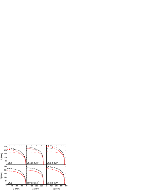
Figure 2: Set 1: Phase Diagrams for several values of the magnetic field. Upper panels correspond to the PNJL model, while lower ones to the EPNJL model. Dashed lines correspond to the chiral restoration crossover while full line to the 1st order one. Dotted lines correspond to the deconfinement transition. In each panel, upper (black) lines correspond to $T_{0}=270$ MeV while lower (red) ones to $T_{0}=208$ MeV.

The behaviour of the CEP is seen in Fig.3. $T_{CEP}$ increases with magnetic field, while $\mu_{CEP}$ tends to decrease, presenting small oscillations. Similar results have been found in the NJL model[9].

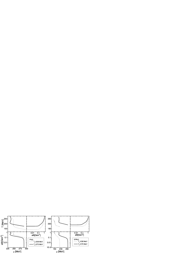
Figure 3: Set 1: Position of CEP as a function of Magnetic Field

In the phase diagram of Set 2 (Fig.4), it is seen that at values around $eB=0.1$ GeV² chiral restoration at low $T$ occurs in several steps: a main transition and two secondary ones, that also turn to crossovers at a CEP. In the EPNJL case (lower panel), there is more than one CEP in the main transition. In Fig.5, the response to magnetic field of all the encountered CEPs is shown. In the PNJL case (left panel), it is seen that there is one CEP at $B=0$, that moves towards the $T=0$ axis when $B$ increases, while the CEP corresponding to one of the secondary transitions moves to higher $T$ values and remains for higher $B$, turning into the main transition CEP. The situation in the EPNJL model(right panel) is much more complicated: at $eB=0.079$ GeV² a pair of CEPs is formed, one of them disappearing after encountering a CEP of one of the secondary transitions, while the other one disappears in the $T=0$ axis. The CEP at $B=0$ remains as the main CEP for all values of $B$.

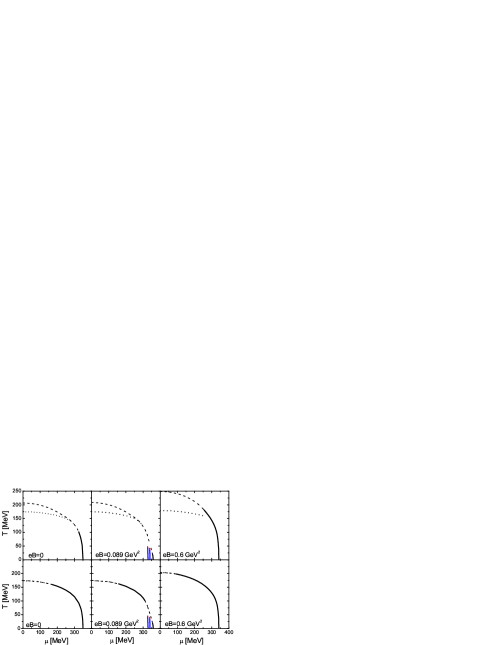
Figure 4: Set 2: Phase Diagrams for several values of the magnetic field. Upper panels correspond to the PNJL model, while lower ones to the EPNJL model. Dashed lines correspond to the chiral restoration crossover while full line to the 1st order one. Dotted lines correspond to the deconfinement transition. Results using $T_{0}=212(190)$ MeV for PNJL (EPNJL) are shown.

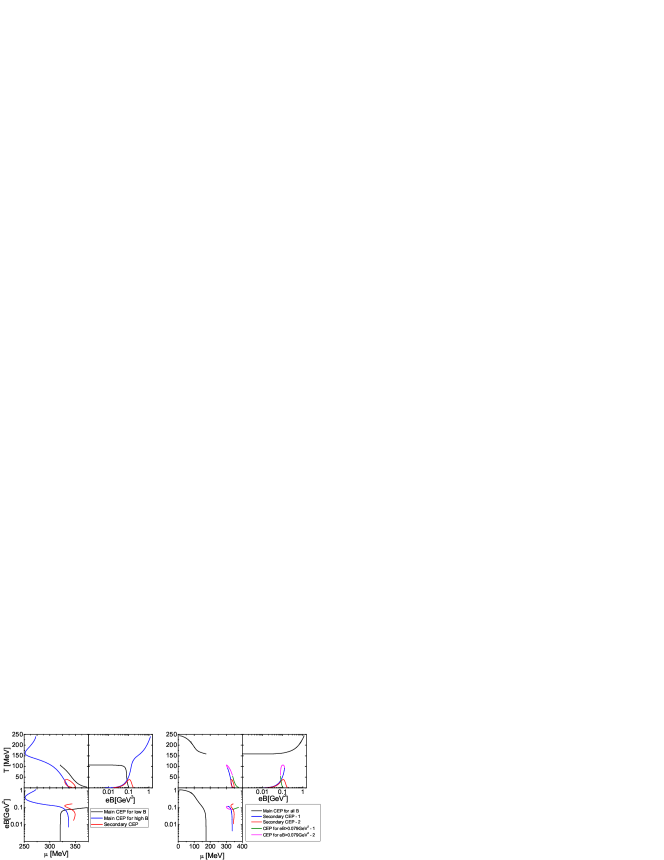
Figure 5: Set 2: Position of CEP as a function of magnetic field. Values of $T_{0}$ as in Fig.4.

4 Conclusions

We have analyzed the effect of an intense magnetic field on the phase diagram of strongly interacting matter as described by (E)PNJL-type models. These models provide a simultaneous dynamical description of the deconfinement and chiral transitions. They are able to describe the enhancement of the chiral condensate with $B$ at $T=\mu=0$. However, as most of the present available models, in their present version they fail to reproduce the inverse magnetic catalysis at finite temperature recently found in lattice QCD. In the EPNJL model there is no splitting at $\mu=0$ between chiral restoration and deconfinement transitions as functions of $B$. Similarly for a given $B$ both transitions coincide up to the critical point. The detailed form of the phase diagram depends, particularly at low $T$, on the quark sector parametrization. For parametrizations leading to a $T=\mu=0$ dressed quark mass smaller than $\simeq 350MeV$ (as in Set 2) there is a quite rich structure due to the subsequent population of the Landau levels as $\mu$ increases. In particular, several CEPs are found.

This work has been partially funded by CONICET (Argentina) under grants # PIP 00682, and by ANPCyT (Argentina) under grant # PICT11 03-113.

References

- [1] D. Kharzeev et al. (Eds.) Strongly Interacting Matter in Magnetic Fields. Lecture Notes in Physics, Vol. 871 (Springer Verlag, Berlin, 2013).
- [2] K. Fukushima, Phys. Lett. B591, 277 (2004); C. Ratti, M. A. Thaler, and W. Weise, Phys. Rev. D 73, 014019 (2006); E. Megias, E. Ruiz Arriola and L. L. Salcedo, Phys. Rev. D 74, 065005 (2006).
- [3] Y. Sakai, T. Sasaki, H. Kouno, and M. Yahiro, Phys. Rev. D 82, 076003 (2010).
- [4] K. Fukushima, M. Ruggieri and R. Gatto, Phys. Rev. D 81, 114031 (2010); R. Gatto and M. Ruggieri, Phys. Rev. D 83, 034016 (2011).
- [5] U. Vogl and W. Weise, Prog. Part. Nucl. Phys. 27 195 (1991); S. Klevansky, Rev. Mod. Phys. 64, 649 (1992); T. Hatsuda and T. Kunihiro, Phys. Rep. 247 221 (1994).
- [6] S. Roessner, C. Ratti and W. Weise, Phys. Rev. D 75, 034007 (2007).
- [7] B.-J. Schaefer, J.M. Pawlowski and J. Wambach, Phys. Rev. D 76 074023 (2007).
- [8] G. S. Bali et al., J. High Energy Phys. 02, 044 (2012).
- [9] S. S. Avancini et al., Phys. Rev. D 85, 091901 (2012).