The Influence of Spatial Variation in Chromatin Density Determined by X-ray Tomograms on the Time to Find DNA Binding Sites

Abstract

In this work we examine how volume exclusion caused by regions of high chromatin density might influence the time required for proteins to find specific DNA binding sites. The spatial variation of chromatin density within mouse olfactory sensory neurons is determined from soft X-ray tomography reconstructions of five nuclei. We show that there is a division of the nuclear space into regions of low-density euchromatin and high-density heterochromatin. Volume exclusion experienced by a diffusing protein caused by this varying density of chromatin is modeled by a repulsive potential. The value of the potential at a given point in space is chosen to be proportional to the density of chromatin at that location. The constant of proportionality, called the volume exclusivity, provides a model parameter that determines the strength of volume exclusion. Numerical simulations demonstrate that the mean time for a protein to locate a binding site localized in euchromatin is minimized for a finite, non-zero volume exclusivity. For binding sites in heterochromatin, the mean time is minimized when the volume exclusivity is zero (the protein experiences no volume exclusion). An analytical theory is developed to explain these results. The theory suggests that for binding sites in euchromatin there is an optimal level of volume exclusivity that balances a reduction in the volume searched in finding the binding site, with the height of effective potential barriers the protein must cross during the search process.

I Introduction

What mechanisms drive the process by which regulatory proteins and transcription factors search for specific DNA binding sites? It is usually assumed that in the absence of any interactions, within an “empty” nucleus a protein will move by Brownian motion and bind upon getting sufficiently close to a target site. This corresponds to the well-known diffusion-limited reaction model of Smoluchowski SmoluchowskiDiffLimRx . A number of theoretical and experimental studies suggest proteins may experience facilitated diffusion, allowing them to find specific binding sites faster than the diffusion limit predicted by the Smoluchowski theory HalfordBindRatesAreDiffLim09 ; NormannoSearchRev2012 . Whether facilitated diffusion occurs in any meaningful way in vivo, allowing proteins to find binding sites significantly faster than the diffusion limit, is very much an active area of investigation and debate HalfordBindRatesAreDiffLim09 ; NormannoSearchRev2012 ; NudlerNatStruct2013 ; VekslerSpeedSelect2013 . In the present paper, we consider the possible influence of volume exclusion caused by spatial heterogeneity in chromatin density on the time needed for a protein to find a target by diffusion.

There are many different interactions that have been proposed that could in principle decrease the mean time required for regulatory proteins and transcription factors to find specific DNA binding sites, relative to the diffusion limited reaction model. These include non-specific DNA binding interactions, electrostatic interactions between proteins and binding sites, one-dimensional diffusion of proteins along DNA, and jumping of proteins between different regions of DNA fibers HalfordBindRatesAreDiffLim09 ; NormannoSearchRev2012 . The relative contribution of these (possible) interactions is still being assessed by both experimental and theoretical studies. Perhaps the most popular of these mechanisms is the possibility that proteins may exploit non-specific DNA binding interactions to allow diffusion or sliding along DNA. In the classic study of Berg et al BergSlidingI , a model was developed in which proteins could undergo a mixed search process involving periods of three-dimensional diffusion, coupled to periods of one-dimensional diffusion along DNA fibers when the proteins were non-specifically bound. A large number of theoretical studies have investigated how this mechanism might influence the search process for specific DNA binding sites (for example, see BergSlidingI ; ElfSingMolSlidingRoadBlocks09 ; HolcmanDNASlide08 ; MirnyDNASlide04 ; MirnySlideGlob09 ; HalfordBindRatesAreDiffLim09 ). Recently, several single-molecule imaging studies have demonstrated that sliding of lac repressor can occur in vivo ElfSingMolSliding07 ; ElfScience2012 . The theoretical estimates in ElfScience2012 suggest this mechanism may allow a significant decrease in the mean time required for a protein to find a specific binding site, in comparison to the diffusion limited reaction model. Most of the existing studies have focused on prokaryotic cells, and it remains to be seen whether sliding along chromatin in eukaryotic cells can noticeably reduce the time required for regulatory proteins to locate specific binding sites in vivo. More complete references for both theoretical models and previous experimental work can be found in the reviews HalfordBindRatesAreDiffLim09 ; NormannoSearchRev2012 .

The nucleus of a eukaryotic cell is a complex spatial environment, containing chromatin fibers with spatially-varying compaction levels, nuclear bodies, and fibrous filaments (such as the nuclear lamina). Spatial inhomogeneity of the nuclear space provides another possible mechanism that may influence the search process of proteins for specific binding sites. In EllenbergVolExEMBOJ09 the impact of spatial variation in chromatin density on the movement of proteins within the nucleus was investigated. Using a combination of single-particle tracking experiments, photo-activation experiments and computational modeling, the authors concluded that chromatin dense regions, such as heterochromatin, exhibited noticeable volume exclusion compared with less dense regions, such as euchromatin. It was observed that similar fluorescence activation curves were found in photo-activation experiments within heterochromatin and euchromatin, when each of the two curves was normalized to the steady-state fluorescence level of its own region. The authors inferred from these experiments that heterochromatin is not substantially more difficult for proteins to enter than euchromatin, but that heterochromatin has a smaller amount of free space in which proteins can accumulate. In contrast, the supplemental movies of RajMRNADiffPNAS2005 demonstrate that individual mRNAs that are able to move freely within nuclei appear restricted to regions of low histone-GFP fluorescence. These mRNAs seem to have difficultly moving into regions of heterochromatin, as identified by regions of high histone-GFP fluorescence.

In IsaacsonPNAS2011 we developed a mathematical model to investigate how the spatially varying density of chromatin within eukaryotic cell nuclei might influence the time required for proteins to find specific binding sites. Our model assumed that regions of higher chromatin density were more difficult for proteins to move into. Protein motion was approximated as diffusion within a volume-excluding potential. The model was constructed from the 3D structured illumination microscopy fluorescence imaging data of GustafsonScience08 . In that work, mouse myoblast cell nuclei were chemically fixed, and both antibody labeled nuclear pores and DAPI stained DNA were imaged. From these data we reconstructed a nuclear membrane surface to determine the nuclear space. The normalized DAPI stain intensity within a given voxel of the imaging data was assumed proportional to the density of chromatin within that voxel. Based on this assumption we constructed a volume exclusion potential, with the value of the potential within a given voxel chosen to be proportional to the normalized DAPI stain intensity of that voxel. The constant of proportionality, which we called the volume exclusivity, was a model parameter that set the overall strength of volume exclusion. By varying the volume exclusivity, we studied how the time to find specific DNA binding sites varied when there was no volume exclusion (i.e. the volume exclusivity was zero and the protein simply diffused), weak volume exclusion, and strong volume exclusion from chromatin dense regions. Numerical simulations of the protein’s search process suggested that for binding sites localized in regions of low DAPI stain intensity, such as the 20th to 30th percentile of intensity values, the median time for proteins to find a specific binding site was minimized for non-zero values of the volume exclusivity. That is, as the volume exclusivity was increased from zero the median binding time initially decreased to a minimum, beyond which the median time increased to infinity. After randomly shuffling the values of the DAPI stain intensity among the voxels of the nucleus, we observed that this effect was lost and the median binding time simply increased as a function of the volume exclusivity. Based on these results, we concluded that the spatial organization of chromatin played a role in the observed minimum of the median binding time for non-zero volume exclusivity. For binding sites localized in regions of high DAPI stain intensity, such as the 70th to 80th percentile of the DAPI stain intensity distribution, the median time to find the binding site increased monotonically as the volume exclusivity was increased from zero.

In this work we expand upon the studies begun in IsaacsonPNAS2011 . To determine chromatin density fields we now use 3D soft X-ray tomography (SXT) reconstructions of cell nuclei McDermott:2009ib ; LarabellCell2012 ; LarabellCell2013 . SXT provides several advantages over fluorescence imaging in assessing the spatial variation of chromatin density. Foremost, the measured linear absorption coefficient (LAC) of a voxel within SXT reconstructions is linearly related to the density of organic material within that voxel by the Beer-Lambert Law McDermott:2009ib . Our simulations in IsaacsonPNAS2011 made use of imaging data from one mouse myoblast cell nucleus, raising the question of whether the observed dependence of the binding time on the volume exclusivity and binding site localization was simply an artifact of the particular cell we studied. In this work we repeat the computational studies of IsaacsonPNAS2011 within five mouse olfactory sensory neuron cell nuclei obtained by SXT imaging. We observe the same qualitative behavior of the mean binding time on volume exclusivity and binding site localization as was observed for the median binding time in IsaacsonPNAS2011 . In addition, we now give a theoretical explanation why the mean binding time has this qualitative behavior.

We begin in the next section by summarizing the SXT imaging data we use in constructing our mathematical models. It is shown that the distribution of LACs within each nucleus is bimodal, indicating a division of the nuclear space into regions with high densities of material and low densities of material. We infer that the lower mode corresponds to the most likely regions of euchromatin, less-compact DNA comprised of the majority of active genes, while the higher mode corresponds to the most likely regions of heterochromatin, more-compact DNA thought to contain most silenced genes AlbertsMOLECELLBIO .

In Section III we summarize the mathematical model we developed in IsaacsonPNAS2011 . The protein is assumed to diffuse in a volume-excluding potential. Since the underlying SXT imaging data is a 3D grid of voxels, we assume the protein’s motion can be approximated by a Markovian continuous-time random walk. The volume exclusion potential within a given voxel is chosen proportional to the normalized LAC of that voxel. The protein moves by hopping between neighboring voxels of the 3D grid with jump rates determined by the protein’s diffusion constant and the strength of the potential difference between the two voxels. Section IV summarizes the underlying stochastic simulation algorithm (SSA) we use to simulate the protein’s search for the binding site.

In Section V we repeat the studies of IsaacsonPNAS2011 using volume exclusion potentials reconstructed from SXT imaging of five cell nuclei. We verify that the conclusions of IsaacsonPNAS2011 still hold in each of the five nuclei, and demonstrate that for binding sites localized in euchromatin, i.e. regions of low chromatin density, volume exclusion can lead to decreases in the mean binding time of $23\%$ to $34\%$ when compared to simulations with no volume excluding potential (zero volume exclusivity). Finally, in Section VI we develop an analytical theory to explain the observed dependence of the mean binding time on the volume exclusivity and binding site localization. The theory suggests that for binding sites in euchromatin there is an optimal level of volume exclusivity that balances a reduction in the volume searched in finding the binding site, with the height of effective potential barriers the protein must cross during the search process.

II Nonuniformity of Nuclear Chromatin Distribution

To measure the spatial variation in chromatin density within nuclei we make use of soft X-ray tomographic (SXT) reconstructions of cells. For an overview of SXT imaging we refer the reader to McDermott:2009ib . In this work we use reconstructions of mouse olfactory sensory neurons, including several mature cells and one immature cell taken from the data of LarabellCell2013 . The experimental protocol for obtaining these reconstructions was the same used in LarabellCell2012 . SXT is similar in concept to medical X-ray CT imaging, but uses soft X-rays in the “water window” which are absorbed by carbon and nitrogen dense organic matter an order of magnitude more strongly than by water McDermott:2009ib . As the absorption process satisfies the Beer-Lambert Law, the measured linear absorption coefficient (LAC) of one voxel of a 3D reconstruction is linearly related to the density of organic material within that voxel McDermott:2009ib . In practice, SXT reconstructions are able to achieve high resolutions of $50\,\textrm{nm}$ or less. For all reconstructions used in this work the underlying voxels were cubes with sides of length $32\,\textrm{nm}$. Another advantage of SXT is in the minimal preprocessing of cells that is required before imaging. Cells are cryogenically preserved, but no segmentation, dehydration, or chemical fixation is necessary. In Appendix A we comment on the measurement error of the SXT imaging process.

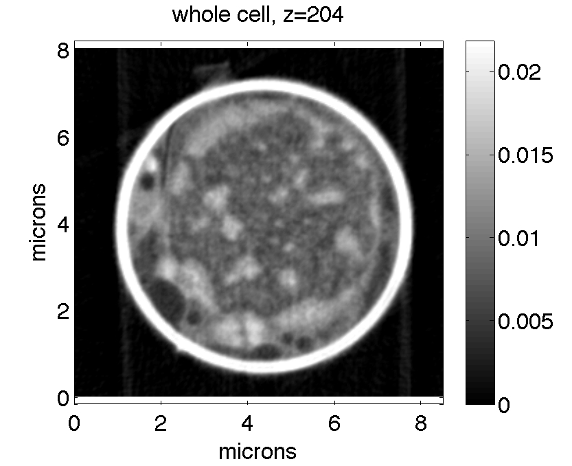
(a)

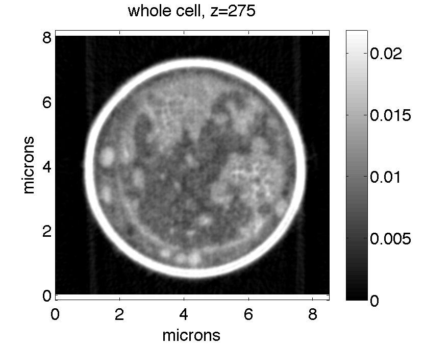
(b)

Figure 1: Reconstructed linear absorption coefficients of a mature mouse olfactory sensory neuron. The cell was cryogenically preserved, and then imaged within a glass capillary (the white ring). (a) and (b) show two $z$-plane slices through the underlying three-dimensional reconstruction. The cell completely fills the capillary in both images. The cell’s nucleus is visible as the circular structure with large regions of lower LAC values (darker pixels). The full 3D reconstruction of this nucleus is shown in Figure 2. In the figures, LACs have units of per voxel. Each LAC value divided by the voxel length of $32\,\textrm{nm}$ would have the more standard units of $\textrm{nm}^{-1}$.

(a)

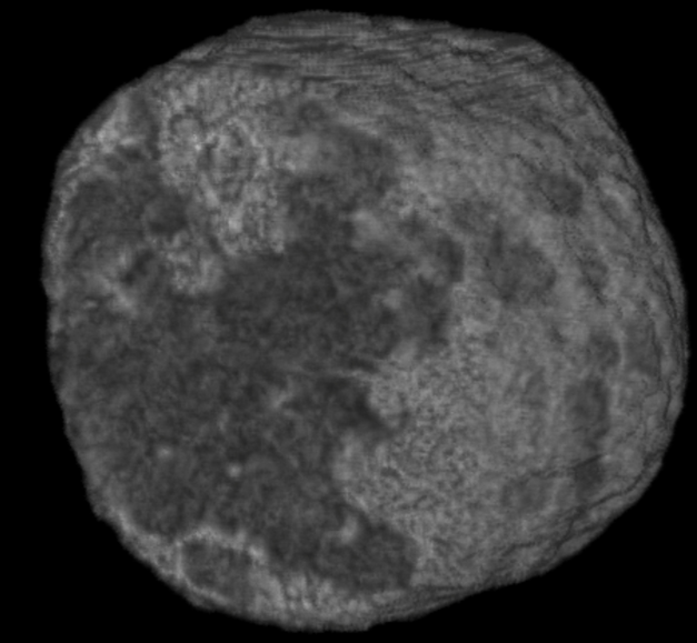
(b)

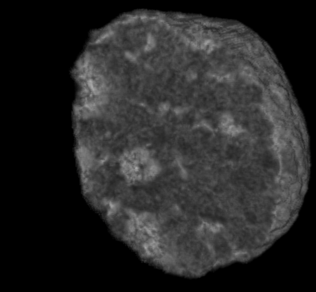
(c)

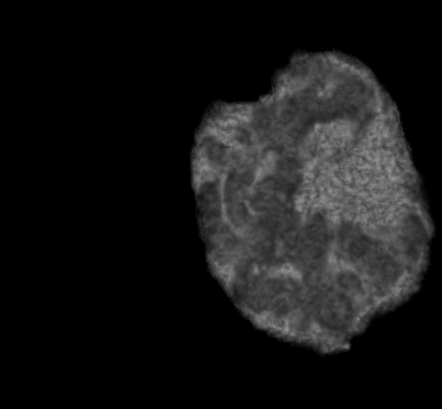
(d)

Figure 2: Nucleus of the cell from Figure 1 (subsequently labeled by “09”). This volume rendering shows the LACs of each voxel of the reconstruction. Lighter colors correspond to larger LACs. (b-d) use clipping planes to reveal the interior of the nucleus along the same axis as used for the full cell and glass capillary reconstructions shown in Figure 1. Movie S1 shows this reconstruction as the clipping plane is moved across the nucleus.

As chromatin is the primary organic material within the nuclei of cells, we subsequently assume the LACs from SXT reconstructions are directly proportional to the density of chromatin within each voxel of the reconstruction. For this reason, in the rest of this paper when we discuss regions of low or high chromatin density we are, more precisely, discussing regions with low or high densities of organic material. In Figure 1 we show two image plane slices through a 3D reconstruction of a cryogenically preserved mature mouse olfactory sensory neuron within a glass capillary. Each image shows the underlying reconstructed LACs within a given voxel, with smaller LACs appearing darker (see colorbars for LAC range). In both images the cell completely fills the capillary, and the cell nucleus is clearly visible as a circular structure within the cell. The full 3D reconstruction of the LACs within the nucleus are shown in Figure 2. Voxels denoting the boundary of the nucleus were hand traced in Amira . From these traces a mask was produced to label voxels within the nucleus. In the rest of this paper the nuclear membrane is assumed to be given by the collection of voxel faces that are shared by a voxel within and a voxel outside the nucleus. It is readily apparent that the nucleus is comprised of regions of low LAC values interspersed with regions of high LAC values. We subsequently identify regions of smaller LACs, corresponding to regions of low density, as euchromatin (regions of less compact DNA, where most active genes are typically located AlbertsMOLECELLBIO ). Regions of higher density are identified as heterochromatin (more compact DNA, often containing silenced genes AlbertsMOLECELLBIO ).

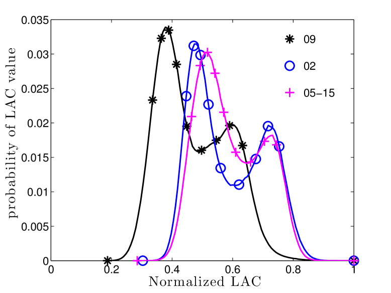
(a)

(b)

Figure 3: Histograms of normalized LAC distribution in the nuclei of five cells. Legends give the label subsequently used to identify each nucleus. For each histogram the LAC values were normalized by the maximum value within that nucleus. Histograms use 100 equally spaced bins between the minimum and maximum normalized LAC values. Markers label every tenth percentile, beginning with the zeroth. Each nucleus is from a mature mouse olfactory sensory neuron, except the 05-15 dataset which was from an immature mouse olfactory sensory neuron. The label for each histogram corresponds to the dataset from LarabellCell2013 from which that nucleus was extracted. The 05-14 dataset contained two cells, with the corresponding nuclei labeled by 05-14-1 and 05-14-2.

Figure 3 provides further motivation for this labeling. There we plot histograms of the normalized LAC distribution within the nuclei of five cells. (By normalized we mean that the LACs have been rescaled so that the maximum LAC within each nucleus is one.) For each nucleus the normalized LAC distribution is bimodal, illustrating the division of the nucleus into regions of euchromatin and heterochromatin. Moreover, we see that the first mode of the distribution occurs between the 20th and 30th percentiles of the normalized LAC distribution, while the second mode occurs between the 70th and 90th percentiles. We therefore interpret these percentile ranges as the most likely LACs for euchromatin and heterochromatin respectively. Note, the bimodal LAC distribution observed in each nucleus is fundamentally different than the unimodal DAPI stain fluorescence distribution we saw in IsaacsonPNAS2011 (which was peaked at zero intensity, see Figure 1C of IsaacsonPNAS2011 ).

III Mathematical Model

We are interested in studying the statistics of the time required for a diffusing regulatory protein to find specific binding sites within the nucleus of a eukaryotic cell. The mathematical model and biological assumptions we describe in this section are based on the model we developed in IsaacsonPNAS2011 . For completeness we summarize them here, but refer the reader to IsaacsonPNAS2011 for further detail.

We assume that in the absence of chromatin, inside the nucleus the protein would move by Brownian motion with a fixed diffusivity. Volume exclusion caused by the varying spatial density of chromatin is modeled by a repulsive potential that imparts drift to the protein’s movement. The strength of the potential is assumed to be proportional to the density of chromatin at a given point in space. Regions of higher chromatin density will therefore be more volume excluding, i.e. more difficult for proteins to enter, than regions of low density. Note, there are many other possible interactions that may influence the protein’s search process. These include non-specific DNA binding interactions, trapping caused by such interactions or local chromatin structure, and the possibility of protein diffusion along DNA HalfordBindRatesAreDiffLim09 ; ElfSingMolSliding07 . The model we describe focuses on how the search process for specific binding sites is influenced by the assumption that regions of high DNA density are more difficult to enter.

As described in the previous section, the measured soft X-ray tomography (SXT) linear absorption coefficients (LACs) are directly proportional to the density of organic matter within a given voxel. We assume here that the LAC gives a direct measure of the density of chromatin in a voxel. Let $I\subset\mathbb{Z}^{3}$ denote the set of voxels from a SXT reconstruction that comprise the nucleus of a cell. For $\boldsymbol{i}\in I$ a given voxel within the nucleus, we denote by $\ell_{\boldsymbol{i}}$ the normalized LAC for that voxel. By normalized we mean that the $\ell$ has been rescaled so that $\max_{\boldsymbol{i}\in I}\ell_{\boldsymbol{i}}=1$. We assume the potential of the $\boldsymbol{i}$th voxel is given by

$$\phi_{\boldsymbol{i}}=\phi_{\textrm{max}}\ell_{\boldsymbol{i}},$$ (1)

where the potential maximum $\phi_{\textrm{max}}$, subsequently called the volume exclusivity, is a parameter of our model. When $\phi_{\textrm{max}}=0$ the particle will simply diffuse, while as $\phi_{\textrm{max}}\to\infty$ it will become increasingly difficult for the protein to enter regions of high chromatin density.

As the imaging data are defined by a mesh of voxels, we approximate the diffusion of the protein within the nucleus as a Markovian continuous-time random walk among these voxels. The protein moves by hopping between neighboring voxels. The probability per unit time that the protein hops from one voxel to a neighbor is determined by the diffusion constant of the protein, the edge length of the voxels, and the strength of the potential barrier crossed in hopping from one voxel to another. Let $P_{\boldsymbol{i}}(t)$ label the probability the protein is in the $\boldsymbol{i}$th voxel at time $t$. In what follows we assume the DNA binding site is given by one specific voxel of the mesh, $\boldsymbol{i}_{\textrm{b}}$, and that upon reaching this voxel the protein immediately binds. Using this condition, our model can be interpreted as an approximation of the search process by the protein for a small region containing the binding site (i.e. the voxel $\boldsymbol{i}_{\textrm{b}}$). The binding reaction then gives the reactive boundary condition that

$$P_{\boldsymbol{i}_{\textrm{b}}}(t)=0.$$ (2)

Note, this choice of boundary condition assumes the protein is immediately removed from the system upon hopping into the voxel containing the binding site. This is equivalent, insofar as the rest of the system is concerned, to the assumption that the protein stays at the binding site once it has arrived there. It is purely a matter of bookkeeping whether we say that the protein is removed from the system upon arrival at the binding site or remains at the binding site once it has arrived there.

Let $\alpha_{\boldsymbol{i}\boldsymbol{j}}$ label the probability per unit time the protein will hop to voxel $\boldsymbol{i}$ when within voxel $\boldsymbol{j}$. The master equation for the probability the protein is in the $\boldsymbol{i}$th voxel at time $t$ is then the linear system of ODEs

$$\frac{dP_{\boldsymbol{i}}}{dt}(t)=\sum_{\boldsymbol{j}\in I}\alpha_{\boldsymbol{i}\boldsymbol{j}}P_{\boldsymbol{j}}(t)-\alpha_{\boldsymbol{j}\boldsymbol{i}}P_{\boldsymbol{i}}(t),\quad\forall\boldsymbol{i}\in I-\{\boldsymbol{i}_{\textrm{b}}\},$$ (3)

where $I-\{\boldsymbol{i}_{\textrm{b}}\}$ denotes the set of voxels, $I$, with the $\boldsymbol{i}_{\textrm{b}}$ voxel removed. Note this model implicitly enforces the no-flux boundary condition that the protein can not leave the nucleus.

The spatial hopping rates $\alpha_{\boldsymbol{i}\boldsymbol{j}}$ were derived in the supplement to IsaacsonPNAS2011 . They are chosen so that in the absence of the reactive boundary condition (2), the master equation (3) would converge as the voxel size approaches zero to a Fokker-Planck partial differential equation (PDE) describing the drift-diffusion of the protein. Let $D$ the diffusion constant of the protein, $h$ the edge length of each voxel, $k_{\text{B}}$ Boltzmann’s constant, and $T$ the temperature of the nucleus. We found in IsaacsonPNAS2011 that when $\boldsymbol{i}$ and $\boldsymbol{j}$ are nearest neighbor voxels along a coordinate axis the choice

$$\alpha_{\boldsymbol{i}\boldsymbol{j}}=\frac{2D}{h^{2}}\frac{1}{\exp((\phi_{\boldsymbol{i}}-\phi_{\boldsymbol{j}})/k_{\text{B}}T)+1},$$ (4)

with $\alpha_{\boldsymbol{i}\boldsymbol{j}}=0$ for all other voxel pairs, provides a second order spatial discretization of the corresponding Fokker-Planck PDE. As the potential barrier to hop from voxel $\boldsymbol{j}$ to $\boldsymbol{i}$ grows ($\phi_{\boldsymbol{i}}-\phi_{\boldsymbol{j}}\to\infty$), we see that $\alpha_{\boldsymbol{i}\boldsymbol{j}}\to 0$. As the potential becomes constant ($\phi_{\boldsymbol{i}}-\phi_{\boldsymbol{j}}\to 0$), we recover a discretization of the standard discrete Laplacian with the corresponding jump rates

$$\alpha_{\boldsymbol{i}\boldsymbol{j}}=\frac{D}{h^{2}}.$$

Note the not-quite-obvious consequence of (4) that

$$\frac{\alpha_{\boldsymbol{i}\boldsymbol{j}}}{\alpha_{\boldsymbol{j}\boldsymbol{i}}}=e^{-\left(\phi_{\boldsymbol{i}}-\phi_{\boldsymbol{j}}\right)/k_{\text{B}}T}.$$

This ensures that the steady state solution to (3), in the absence of the reactive boundary condition (2), is the discrete Gibbs-Boltzmann distribution

$$P^{\textrm{ss}}_{\boldsymbol{i}}=\frac{e^{-\phi_{\boldsymbol{i}}/k_{\text{B}}T}}{\sum_{\boldsymbol{j}\in I}e^{-\phi_{\boldsymbol{j}}/k_{\text{B}}T}}.$$ (5)

This steady-state will be used in Section VI to estimate the explicit dependence on $\phi_{\textrm{max}}$ of the mean time for the protein to find the binding site, $\boldsymbol{i}_{\textrm{b}}$.

We assume that the protein begins its search for the binding site from a nuclear pore within the nuclear membrane. As nuclear pores are not explicitly visible by soft X-ray tomography, we make the approximation that each voxel on the border of the nucleus contains the same fraction of the total number of nuclear pores. Instead of studying the protein’s search from one specific pore (voxel), at the start of each individual simulation we choose the protein’s initial position from a uniform distribution among all voxels on the border of the nucleus. The corresponding initial condition for the master equation (3) is therefore

$$P_{\boldsymbol{i}}(0)=\begin{cases}\frac{1}{N_{\textrm{bnd}}},\quad\boldsymbol{i}\in I_{\textrm{bnd}},\\ 0,\quad\boldsymbol{i}\notin I_{\textrm{bnd}},\end{cases}$$ (6)

where $I_{\textrm{bnd}}$ labels the set of voxels on the boundary of the nucleus and $N_{\textrm{bnd}}$ denotes the number of voxels in this set.

We shall also investigate an extension of the preceding model where $\boldsymbol{i}_{\textrm{b}}$ is allowed to be a random variable. To understand the difference in binding times for binding sites localized in euchromatin versus heterochromatin, we allow $\boldsymbol{i}_{\textrm{b}}$ to be chosen from a uniform distribution among all voxels with LACs between two specified percentiles of the nuclear LAC distribution. Binding sites placed in euchromatin were chosen from low percentiles, usually the 20th to 30th, near the first mode of the LAC distribution (see Figure 3). For the fluorescence imaging data we used in IsaacsonPNAS2011 , this percentile range corresponded to the first in which there was a non-zero fluorescence level. For the SXT data this range represents the most likely LAC values for euchromatin containing voxels. (It is unknown if voxels with sufficiently low LAC values actually contain chromatin. Similarly, it has yet to be determined experimentally if there is a precise LAC value above which voxels may be assumed to contain heterochromatin.) To model heterochromatin we used higher percentiles near the second mode, such as the 70th to 80th.

IV Numerical Solution Method

For a specified value of $\boldsymbol{i}_{\textrm{b}}$, the master equation (3) with boundary condition (2) and initial condition (6) is a linear system of ODEs. A typical reconstruction of a nucleus contains on the order of 2.7 million voxels (slightly more than would be contained in a 128 by 128 by 128 Cartesian mesh). While such a system of ODEs can be solved directly, allowing $\boldsymbol{i}_{\textrm{b}}$ to be a random variable would potentially require the system to be solved many times to obtain good statistical estimates of the binding times. For this reason we simulated the underlying continuous-time random walk of the protein between the voxels instead of directly solving (3). In these simulations the protein hops from voxel $\boldsymbol{i}$ to neighbor $\boldsymbol{j}$ with probability per unit time $\alpha_{\boldsymbol{j}\boldsymbol{i}}$. When the protein hops into the voxel containing the binding site, $\boldsymbol{i}_{\textrm{b}}$, the simulation is terminated and the time the protein entered the voxel recorded. Exact realizations of this stochastic process can be generated by the stochastic simulation algorithm (SSA), also known as the Gillespie method or Kinetic Monte Carlo GillespieJPCHEM1977 ; KalosKMC75 ; GibsonBruckJPCHEM2002 .

Our numerical simulation algorithm can be summarized as follows

1. Pre-calculate the jump rates, $\alpha_{\boldsymbol{i}\boldsymbol{j}}$.

2. Choose the binding site location, $\boldsymbol{i}_{\textrm{b}}$. This is either specified, or sampled from voxels within specified percentiles of the LAC distribution (i.e. euchromatin or heterochromatin regions).

3. Sample the initial position of the protein from $P_{\boldsymbol{i}}(0)$.

4. Use the SSA to simulate the motion of the protein until the time, $\tau$, that it hops into the voxel $\boldsymbol{i}_{\textrm{b}}$.

5. Repeat from step 2 until the desired number of simulations have been run.

V Mean Time to Find a DNA Binding Site

We now investigate the statistics of the first passage time, $\tau$, for the protein to find the binding site, and how these statistics depend on the binding site position and volume exclusivity, $\phi_{\textrm{max}}$. We focus on the survival probability that the protein has not found the binding site by time $t$,

$$\operatorname{Pr}\left[\tau>t\right]=\sum_{\boldsymbol{i}\in I}P_{\boldsymbol{i}}(t),$$

and the mean binding time

$$\mathbb{E}[\tau]=\int_{0}^{\infty}\operatorname{Pr}\left[\tau>t\right]\,dt.$$

For all reported simulations, $\operatorname{Pr}\left[\tau>t\right]$ and associated $95\%$ confidence intervals were estimated using MATLAB’s ecdf routine. $\mathbb{E}[\tau]$ and associated confidence intervals were estimated using MATLAB’s mean routine, while the standard error was estimated using standard deviations determined by MATLAB’s std routine.

In the following we choose $D=10\,\mu\textrm{m}^{2}\textrm{s}^{-1}$, and report $\phi_{\textrm{max}}$ in units of $k_{\text{B}}T$. For each SXT reconstruction the voxels were cubic with edge length $32\,\textrm{nm}$. In all simulations spatial units were in $\mu\text{m}$, so that $h=.032\,\mu\text{m}$, and time had units of seconds.

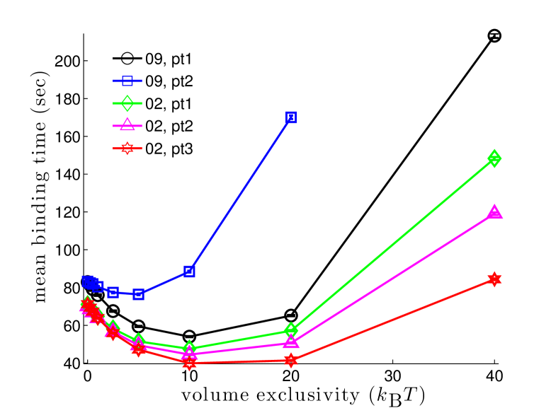
(a)

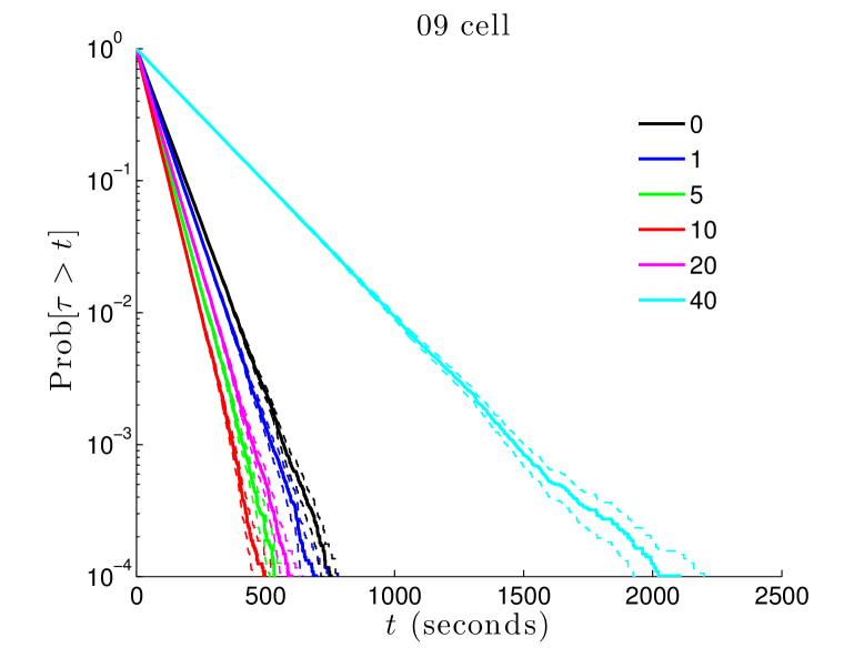
(b)

Figure 4: Mean binding time and survival time distribution for binding sites at fixed locations in euchromatin. (a) Mean binding time as the volume exclusivity, $\phi_{\textrm{max}}$, is varied. Inset gives the cell nucleus and target point label for each curve. Each data point was obtained from 128000 simulations. $95\%$ confidence intervals are shown for each point, but often smaller than the marker size. As $\phi_{\textrm{max}}$ is increased we see each curve initially approaches a minimum before diverging to $\infty$. (b) Survival time distribution for the “pt1” binding site from the 09 cell nucleus. The inset gives the volume exclusivity, $\phi_{\textrm{max}}$, in units of $k_{\text{B}}T$. Each curve was generated from binding time statistics for 128000 simulations. The dashed lines about each solid curve give $95\%$ confidence intervals. Linearity of $\operatorname{Pr}\left[\tau>t\right]$ with the logarithmic $y$-axis suggests the binding time is approximately exponential.

We first examined the time to find a fixed binding site within regions of euchromatin. Several voxels within the euchromatin regions of the 09 and 02 cell nuclei were sampled randomly from all voxels in the 20th to 30th percentiles of the nuclear LAC distribution (see Figure 3). For each fixed binding site 128000 simulations were run, and the time that the protein first encountered the binding site was recorded. In Figure 4 we examine the statistics of the binding time, $\tau$, for five different binding sites within two cell nuclei (labeled by “09, pt1”, “09, pt2”, “02, pt1”, “02, pt2”, and “02, pt3”). Figure 4a shows the mean binding time as a function of $\phi_{\textrm{max}}$ for each of the five binding sites. We see that as the volume exclusivity is increased from zero the mean binding time decreases to a minimum. As the volume exclusivity is further increased the mean binding time then increases dramatically. This behavior can also be seen in Figure 4b, where we show the survival time distribution for the binding site “pt1” from the 09 cell nucleus as the volume exclusivity, $\phi_{\textrm{max}}$, is increased. Notice that each curve is linear with a logarithmic $y$-axis, suggesting that the time to find the binding site is approximately an exponential random variable.

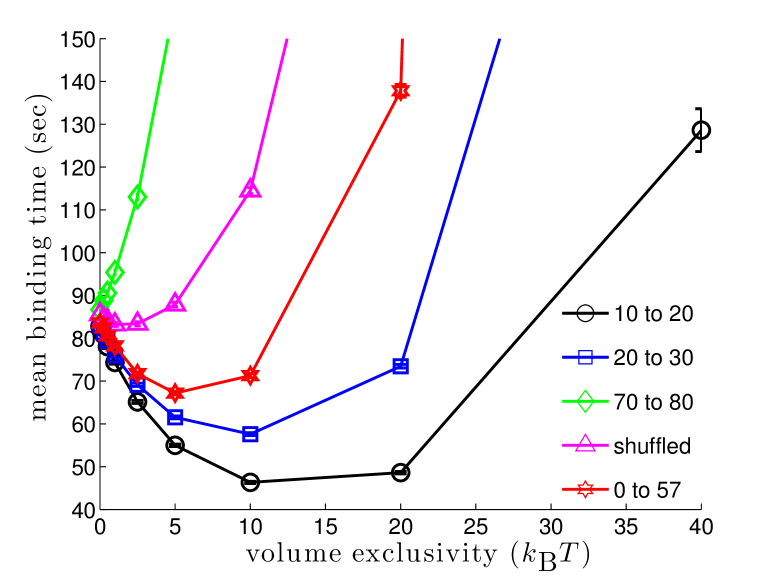
(a)

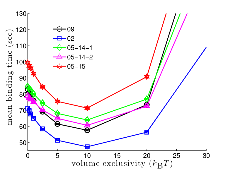
(b)

Figure 5: Mean binding time for binding sites randomly localized in subsets of the nucleus as the volume exclusivity is varied. For each simulation the target binding site was sampled from a uniform distribution among all voxels within fixed percentile ranges of the nuclear LAC distribution. Each data point was calculated from 128000 simulations. (a) Mean binding times in the 09 cell. The inset gives the percentile range used for each curve. The black (10 to 20) and blue (20 to 30) curves localized binding sites in regions of euchromatin, see Figure 3a. The red (0 to 57) curve localized binding sites anywhere before the LAC value giving the minimum between the two modes of the LAC distribution. The green (70 to 80) curve localized binding sites in heterochromatin. For the magenta curve the values of the LAC distribution were randomly shuffled among the voxels of the nucleus. Binding sites were then chosen from a uniform distribution among voxels with LAC values in the 20th to 30th percentiles of the LAC distribution. For binding sites in heterochromatin, or when using the shuffled potential, the mean binding time diverges as the volume exclusivity is increased. (b) Mean binding times for binding sites randomly chosen at the start of each simulation within the 20th to 30th percentile of the LAC distribution for five different cell nuclei. For each cell, binding sites in euchromatin were found fastest when $\phi_{\textrm{max}}\approx 10\,k_{\text{B}}T$.

Figures 5 and 6 show how the binding time varies when the binding site is localized in different subregions of the nucleus. For each value of $\phi_{\textrm{max}}$, a percentile range of the LAC distribution was specified and 128000 simulations were run. At the beginning of each simulation the binding site was sampled from a uniform distribution among all voxels within the percentile range. As such, the figures illustrate the average of the mean binding time and survival probability distribution over binding sites localized in different percentile ranges of the LAC distribution. Figure 5a illustrates how the mean binding time varies in the 09 nucleus as a function of $\phi_{\textrm{max}}$ when binding sites were localized in euchromatin (the 10th to 20th and 20th to 30th percentile ranges) versus heterochromatin (the 70th to 80th percentile range). When the binding site was localized in regions of higher chromatin density the mean binding time increased. Moreover, while localizing the binding site within euchromatin leads to a minimum in the mean binding time for non-zero volume exclusivity (about $10\,k_{\text{B}}T$), this behavior is lost for binding sites localized in heterochromatin. For the latter the mean binding time simply increases as $\phi_{\textrm{max}}$ increases. Figure 5b illustrates that the appearance of a minimum for non-zero volume exclusivity when binding sites are in regions of euchromatin (20th to 30th percentile range) persists across all five of the nuclei we studied. Moreover, for each nucleus the minimum appears at $\phi_{\textrm{max}}\approx 10\,k_{\text{B}}T$.

The preceding simulations focused on binding sites localized near the most likely regions of euchromatin and heterochromatin. We also examined the behavior of the binding time for binding sites localized in broader regions. The zeroth to 57th percentile curve in Figure 5a corresponds to localizing the binding site anywhere before the minimum located between the two modes of the LAC distribution of the 09 cell, see Figure 3a. This minimum was defined to be the center of the bin between the two modes of the 09 nucleus histogram in Figure 3a that had the smallest height, approximately the 57th percentile of the LAC distribution. In LarabellCell2013 , the transition point between euchromatin and heterochromatin was assumed to be given by averaging the LAC values at the two modes. For the 09 nucleus, this transition point differs from the location of the minimum between the two modes by less than $.1\%$. Figure 5a shows that within this broader region a minimal mean binding time still occurs for a nonzero value of the volume exclusivity, but the overall decrease in the mean binding time relative to that when the volume exclusivity is zero is smaller than for binding sites localized near the mode (20th to 30th percentile). In particular, for sites sampled from the zeroth to 57th percentile range we observe that the smallest mean binding time is $20\%$ faster than that when the volume exclusivity is zero, while for sites sampled from the 20th to 30th percentile range the smallest mean binding time is $31\%$ faster. This decrease in the observed speed-up of the mean binding time arises from the substantially longer time needed to find binding sites within voxels having the highest LAC values. The smallest median binding time, which is less sensitive to outliers, is $27\%$ faster than the median binding time with zero volume exclusivity for binding sites in the zeroth to 57th percentile range (compared to $31\%$ faster for the 20th to 30th percentile range).

To test whether the minimum for binding sites in euchromatin regions was dependent on the spatial structure of the LAC distribution we randomly shuffled the values of the LAC distribution among the voxels of the 09 cell nucleus. This preserved the overall distribution of LAC values, shown in Figure 3a, while removing all spatial correlations between the values in neighboring voxels. As seen in Figure 5a, for binding sites in euchromatin (the 20th to 30th percentile range), the occurrence of a minimum mean binding time for non-zero volume exclusivity is lost (magenta curve). We discuss this result further in the next section, where we show the appearance of a minimum is to be expected if the potential is slowly varying relative to the length scale of the binding site.

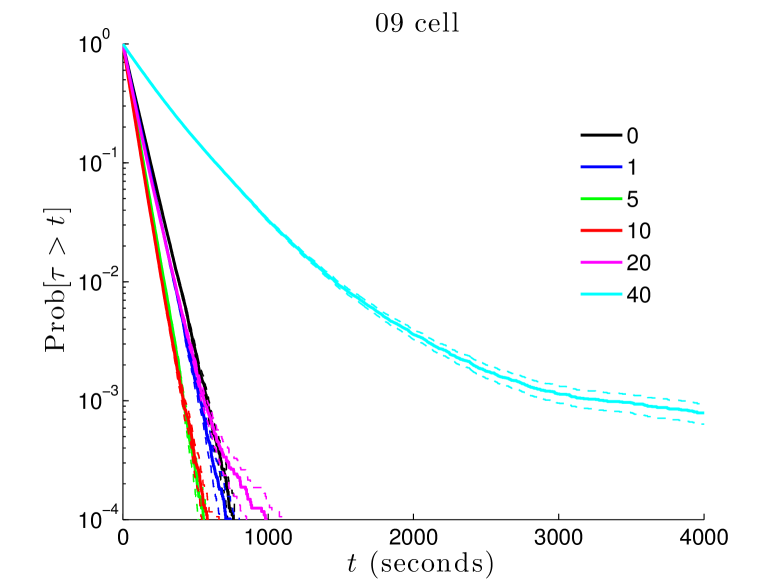
(a)

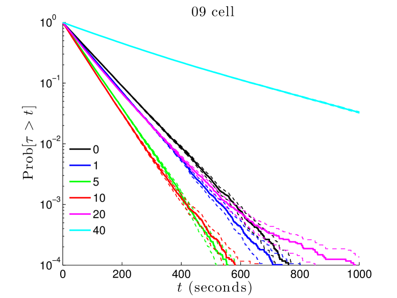
(b)

Figure 6: Survival time distributions for binding sites randomly localized in euchromatin. For each simulation one voxel in euchromatin (the 20th to 30th percentile of the LAC distribution) is randomly chosen to represent the binding site. Each curve is then estimated from 128000 such simulations. Insets give the volume exclusivity, $\phi_{\textrm{max}}$, for every curve. (a) For large values of the volume exclusivity the survival probability is no longer well-approximated by an exponential distribution for all times. (b) Reducing the scale of the $t$-axis we can see that as $\phi_{\textrm{max}}$ is increased the survival distribution initially shits to the left, leading to faster binding times. As $\phi_{\textrm{max}}\to\infty$ the distribution shifts back to the right.

In Figure 6 we show the survival distributions, $\operatorname{Pr}\left[\tau>t\right]$, for the 09 cell nucleus when for each simulation the binding site was randomly localized in regions of euchromatin (20th to 30th percentile range). Note that for large values of the volume exclusivity the survival probability is no longer well-approximated by an exponential distribution, in contrast to the case in which the binding site was fixed across all simulations (as in Figure 4b). This non-exponential behavior arises because the binding site location is now itself a random variable. Figure 6b uses an expanded $t$-axis from Figure 6a to illustrate how the survival distribution shifts as the volume exclusivity is increased. We see that initially the distribution shifts to the left, leading to faster binding times, but that as $\phi_{\textrm{max}}\to\infty$ the distribution rapidly shifts rightward.

Nucleus	09	02	05-14-1	05-14-2	05-15	SIM nucleus
Percent Speedup	31%	34%	24%	23%	28%	33%

Table 1: Percent difference between mean binding time with no volume exclusion ($\phi_{\textrm{max}}=0$) and the smallest mean binding time as $\phi_{\textrm{max}}$ is varied (from Figure 5b). The last column gives the percent speed up in the median binding time we found for a single mouse myoblast cell nucleus reconstructed from structured illumination microscopy (SIM) of DAPI stained DNA IsaacsonPNAS2011 . The corresponding speedup in median binding times for the X-ray tomography data we study here was comparable to the values reported for the means above.

The results of this section are consistent with those we found when studying a single cell in IsaacsonPNAS2011 using a chromatin density field reconstructed from fluorescence imaging of DAPI stained DNA. Our new simulations illustrate that across several cells of different phenotypes these results persist. The use of X-ray tomography provides a more direct measure of chromatin density since each voxel’s LAC is directly proportional to the density of organic material within that voxel McDermott:2009ib . Thus, we would expect the present results to capture more accurately the true spatial distribution of chromatin within each nucleus. Across the five nuclei of this paper, we see that for binding sites localized in euchromatin volume exclusion can lead to $23\%$ to $34\%$ lower (i.e., faster) mean search times. The maximum observed speedups are summarized in Table 1.

VI Why Does the Mean Binding Time Exhibit a Minimum for Binding Sites in Euchromatin?

In this section we investigate why, for binding sites localized in regions of euchromatin, the mean binding time has a minimum as $\phi_{\textrm{max}}$ is increased from zero to infinity. Our analysis is based on the assumption that near the binding site the volume exclusion potential varies sufficiently slowly that it is well-approximated by a constant.

To estimate the solution to (3) we make several assumptions:

1. There exists a collection of voxels, $I^{\prime}$, about and including the binding site where the potential can be approximated as constant.

2. The portion of the nucleus given by the voxels in $I^{\prime}$ is large in diameter relative to the length of one voxel, but small relative to the diameter of the entire nucleus.

3. The initial position of the protein is outside $I^{\prime}$, that is $P_{\boldsymbol{i}}(0)=0$ for $\boldsymbol{i}\in I^{\prime}$.

4. The solution to (3) reaches a quasi-steady state in space within $I^{\prime}$ faster than the binding time scale. We therefore assume that for $\boldsymbol{i}\in I^{\prime}$, $\frac{dP_{\boldsymbol{i}}}{dt}\approx 0$.

5. The time for the protein to find the binding site is sufficiently large that the solution to (3) outside $I^{\prime}$ is essentially in equilibrium before the protein locates the binding site. In particular, all memory of the initial position is lost.

Using these assumptions we construct two solutions to (3), an inner solution valid near $\boldsymbol{i}_{\textrm{b}}$, $P^{\,\textrm{in}}_{\boldsymbol{i}}(t)$, and an outer solution valid outside $I^{\prime}$, $P^{\,\textrm{out}}_{\boldsymbol{i}}(t)$. The last assumption above implies that

$$P^{\,\textrm{out}}_{\boldsymbol{i}}(t)=A(t)e^{-\phi_{\boldsymbol{i}}/k_{\text{B}}T},\quad\boldsymbol{i}\in I-I^{\prime},$$ (7)

where $A(t)$ is a decreasing function of time, to be determined later. Since, by assumption 1, $\phi_{\boldsymbol{i}}$ is nearly constant on $I^{\prime}$, we can use (7) to extend the definition of $P^{\,\textrm{out}}_{\boldsymbol{i}}$ so that

$$P^{\,\textrm{out}}_{\boldsymbol{i}}(t)=A(t)e^{-\phi_{\boldsymbol{i}_{\textrm{b}}}/k_{\text{B}}T},\quad\boldsymbol{i}\in I^{\prime}.$$ (8)

The second, third, and fourth assumptions imply

$$\sum_{\boldsymbol{j}\in I}\alpha_{\boldsymbol{i}\boldsymbol{j}}P^{\,\textrm{in}}_{\boldsymbol{j}}(t)-\alpha_{\boldsymbol{j}\boldsymbol{i}}P^{\,\textrm{in}}_{\boldsymbol{i}}(t)=0,\quad\forall\boldsymbol{i}\in I^{\prime}-\{\boldsymbol{i}_{\textrm{b}}\},$$ (9)

with the boundary condition $P^{\,\textrm{in}}_{\boldsymbol{i}_{\textrm{b}}}=0$. The assumption that the potential is constant in $I^{\prime}$ then simplifies (9) to

$$D\Delta_{h}P^{\,\textrm{in}}_{\boldsymbol{i}}(t)=\frac{D}{h^{2}}\sum_{d=1}^{3}\left[P^{\,\textrm{in}}_{\boldsymbol{i}+\boldsymbol{e}_{d}}(t)+P^{\,\textrm{in}}_{\boldsymbol{i}-\boldsymbol{e}_{d}}(t)-2P^{\,\textrm{in}}_{\boldsymbol{i}}(t)\right]=0,\quad\boldsymbol{i}\in I^{\prime}-\{\boldsymbol{i}_{\textrm{b}}\},$$ (10)

where $\Delta_{h}$ denotes the discrete Laplacian and $\boldsymbol{e}_{d}$ is a unit vector along the $d$th coordinate axis of $\mathbb{R}^{3}$. This equation is coupled to the boundary condition that $P^{\,\textrm{in}}_{\boldsymbol{i}_{\textrm{b}}}(t)=0$. Finally, we make the standard inner solution assumption (see ColeKevorkianBook ; WardCheviakov2011 ) that $I^{\prime}$ is sufficiently large that the solution to this equation can be approximated by the solution when $I^{\prime}=\mathbb{Z}^{3}$.

If $A(t)$ were known, a unique solution to (10) when $I^{\prime}=\mathbb{Z}^{3}$ could be obtained by specifying the matching condition that

$$\lim_{\left|\boldsymbol{i}\right|\to\infty}P^{\,\textrm{in}}_{\boldsymbol{i}}(t)=P^{\,\textrm{out}}_{\boldsymbol{i}_{\textrm{b}}}(t).$$ (11)

This condition assumes that $I^{\prime}$ looks like a single voxel on length scales of relevance to the outer solution. We note that all time-dependence in (10) arises from this matching condition.

To solve (10) we consider a related problem where the absorbing boundary condition $P^{\,\textrm{in}}_{\boldsymbol{i}_{\textrm{b}}}(t)=0$ is replaced with an explicit sink. Let $C_{\boldsymbol{i}}(t)$ satisfy

$$D\Delta_{h}C_{\boldsymbol{i}}(t)=K(t)\delta_{\boldsymbol{i}\boldsymbol{0}},\quad\boldsymbol{i}\in\mathbb{Z}^{3},$$ (12)

with $\lim_{\left|\boldsymbol{i}\right|\to\infty}C_{\boldsymbol{i}}(t)=0$. Here $K(t)$ denotes the probability per time the protein is removed from the origin at time $t$. The choice $P^{\,\textrm{in}}_{\boldsymbol{i}}(t)=C_{\boldsymbol{i}-\boldsymbol{i}_{\textrm{b}}}(t)-C_{\boldsymbol{0}}(t)$ satisfies (10) with the boundary condition $P^{\,\textrm{in}}_{\boldsymbol{i}_{\textrm{b}}}(t)=0$. Note that $C_{\boldsymbol{i}}(t)\leq 0$, with its most negative value at $\boldsymbol{i}=\boldsymbol{0}$. Therefore $P^{\,\textrm{in}}_{\boldsymbol{i}}(t)\geq 0$, as required. The matching condition (11) then gives

$$\lim_{\left|\boldsymbol{i}\right|\to\infty}P^{\,\textrm{in}}_{\boldsymbol{i}}(t)=-C_{\boldsymbol{0}}(t)=A(t)e^{-\phi_{\boldsymbol{i}_{\textrm{b}}}/k_{\text{B}}T},$$

so that solving for $A(t)$, and substituting the result into (7) and (8) we find

$$P^{\,\textrm{out}}_{\boldsymbol{i}}(t)=-C_{\boldsymbol{0}}(t)e^{\left(\phi_{\boldsymbol{i}_{\textrm{b}}}-\phi_{\boldsymbol{i}}\right)/k_{\text{B}}T}.$$ (13)

$C_{\boldsymbol{0}}(t)$ can be determined using Fourier transforms. Let $B=\left[-\pi,\pi\right]^{3}$ denote the cube centered at the origin with edges of length $2\pi$. Then for $\boldsymbol{\xi}=(\xi_{1},\xi_{2},\xi_{3})$ labeling a point in $B$,

$$C_{\boldsymbol{i}}(t)=\frac{1}{(2\pi)^{3}}\int_{B}\hat{C}(\boldsymbol{\xi},t)\,e^{i(\boldsymbol{i}\cdot\boldsymbol{\xi})}d\boldsymbol{\xi},$$

where $\hat{C}(\boldsymbol{\xi},t)$ denotes the Fourier transform of $C_{\boldsymbol{i}}(t)$ and $i=\sqrt{-1}$. The solution to (12) in Fourier space is easily found to be

$$\hat{C}(\boldsymbol{\xi},t)=-\frac{K(t)h^{2}}{4D}\frac{1}{\sum_{d=1}^{3}\sin^{2}\left(\frac{\xi_{d}}{2}\right)},$$

so that

$$C_{\boldsymbol{0}}(t) =-\frac{K(t)h^{2}}{32\pi^{3}D}\int_{B}\frac{1}{\sum_{d=1}^{3}\sin^{2}\left(\frac{\xi_{d}}{2}\right)}\,d\boldsymbol{\xi},$$

$$=-\frac{2K(t)h^{2}}{\pi^{3}D}\int_{\tilde{B}}\frac{1}{\sum_{d=1}^{3}\sin^{2}\left(\xi_{d}\right)}\,d\boldsymbol{\xi},$$ (14)

where $\tilde{B}=\left[0,\frac{\pi}{2}\right]^{3}$. We note that the singularity of the integrand in (14) is like $\left|\boldsymbol{\xi}\right|^{-2}$, and hence integrable.

To find the distribution of binding times, and in particular the mean binding time, we make the approximation that the survival probability at any given time $t$ can be found from the outer solution alone, i.e., we assume that

$$\operatorname{Pr}\left[\tau>t\right]=\sum_{\boldsymbol{i}\in I}P^{\,\textrm{out}}_{\boldsymbol{i}}(t)=-C_{\boldsymbol{0}}(t)e^{-\phi_{i_{b}}/k_{\text{B}}T}Z,$$

where $Z$ is the partition function

$$Z=\sum_{\boldsymbol{i}\in I}e^{-\phi_{\boldsymbol{i}}/k_{\text{B}}T}.$$

If we substitute $C_{\boldsymbol{0}}(t)$ as given by (14) into the above equation, and if we also recall that $K(t)$ is the probability per unit time of binding, and therefore that

$$K(t)=-\frac{d}{dt}\operatorname{Pr}\left[\tau>t\right]$$

we get

$$\operatorname{Pr}\left[\tau>t\right]=-\mathbb{E}[\tau]\frac{d}{dt}\operatorname{Pr}\left[\tau>t\right]$$ (15)

where

$$\mathbb{E}[\tau]=\frac{2}{\pi^{3}Dh}\left(\sum_{\boldsymbol{i}\in I}e^{\left(\phi_{\boldsymbol{i}_{\textrm{b}}}-\phi_{\boldsymbol{i}}\right)/k_{\text{B}}T}h^{3}\right)\int_{\tilde{B}}\frac{1}{\sum_{d=1}^{3}\sin^{2}\left(\xi_{d}\right)}\,d\boldsymbol{\xi}.$$ (16)

Equation (15) shows that the distribution of binding times is exponential, and (16) gives an explicit formula for the mean binding time, $\mathbb{E}[\tau]$. Note that the theoretical estimate (16) involves no unknown parameters. No parameter fitting is necessary to compare the predicted mean binding time (16) to the simulation results of the previous section.

As the voxel size approaches zero, $\mathbb{E}[\tau]\to\infty$ like $h^{-1}$. This is consistent with the well-known fact that it takes an infinite amount of time for a point particle to find a point target by diffusion in a three-dimensional space. (Recall that our target is one voxel in all of the computations reported here.) As we approach the limit $h\to 0$, the last of our simplifying assumptions becomes more and more valid, since there is more and more time for $P^{\,\textrm{out}}_{\boldsymbol{i}}$ to equilibrate before binding occurs. Related to this, the assumption that the initial position of the protein does not matter also becomes better and better as $h\to 0$.

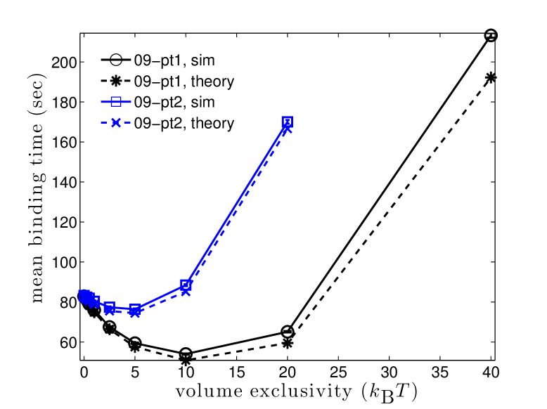
(a)

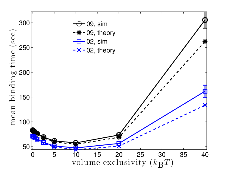
(b)

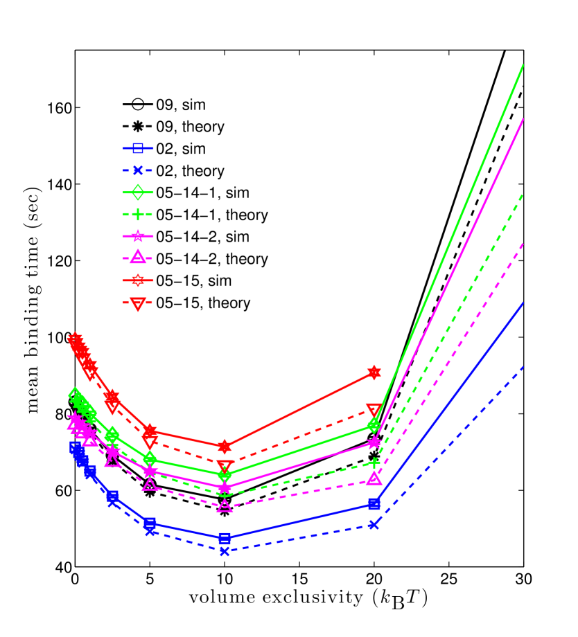
(c)

Figure 7: Theoretical mean binding times (16) and (19) versus those from simulations. Note that both theoretical mean binding times involve no fitting to the simulated times, and are completely determined by known parameters. In all figures solid lines give the mean binding times from simulations, while dashed lines give the corresponding theoretical prediction. (a) 09 cell for the two fixed targets used in Figure 4a. Theoretical mean binding times are from (16). (b) 09 and 02 cells with binding sites randomly localized in euchromatin (20th to 30th percentile of LAC distribution). Simulated means are those from Figure 5b, while theoretical are from (19). (c) All five nuclei when binding sites are randomly localized in regions of euchromatin (20th to 30th percentile of the LAC distribution). Simulated means are the same is in Figure 5b, while theoretical are from (19).

In Figure 7a we compare the mean time to find a target binding site predicted by (16) to the empirical mean times found from the simulations in Figure 4a. The solid curves in Figure 7a show the simulated mean binding times for the two target locations in the 09 cell that were used in Figure 4a. The dashed curves show the estimated mean binding times using (16). The theory gives very good agreement in the predicted mean binding time, particularly for smaller values of the volume exclusivity, $\phi_{\textrm{max}}$.

To see why the mean binding time has a minimum for binding sites in euchromatin regions we look at the behavior of $\mathbb{E}[\tau]$ as $\phi_{\textrm{max}}$ is increased from zero. Let

$$\hat{\tau}=\frac{2h^{2}}{\pi^{3}D}\int_{\tilde{B}}\frac{1}{\sum_{d=1}^{3}\sin^{2}\left(\xi_{d}\right)}\,d\boldsymbol{\xi}.$$

Using (1) we have that

$$\mathbb{E}[\tau]=\hat{\tau}\sum_{\boldsymbol{i}\in I}e^{\phi_{\textrm{max}}\left(\ell_{\boldsymbol{i}_{\textrm{b}}}-\ell_{\boldsymbol{i}}\right)/k_{\text{B}}T},$$ (17)

where $\ell_{\boldsymbol{i}}$ denotes the normalized LAC in voxel $\boldsymbol{i}$. We now consider the mean binding time as a function of $\phi_{\textrm{max}}$, $\mathbb{E}[\tau](\phi_{\textrm{max}})$. Taking the derivative in $\phi_{\textrm{max}}$,

$$\frac{d}{d\phi_{\textrm{max}}}\mathbb{E}[\tau](\phi_{\textrm{max}})=\frac{\hat{\tau}}{k_{\text{B}}T}\sum_{\boldsymbol{i}\in I}\left(\ell_{\boldsymbol{i}_{\textrm{b}}}-\ell_{\boldsymbol{i}}\right)e^{\phi_{\textrm{max}}\left(\ell_{\boldsymbol{i}_{\textrm{b}}}-\ell_{\boldsymbol{i}}\right)/k_{\text{B}}T}.$$

At $\phi_{\textrm{max}}=0$, $\mathbb{E}[\tau](\phi_{\textrm{max}})$ will be decreasing when $\ell_{\boldsymbol{i}_{\textrm{b}}}$ is smaller than the mean of the nuclear LAC distribution, and increasing when $\ell_{\boldsymbol{i}_{\textrm{b}}}$ is above the mean. Examining the second derivative we see

$$\frac{d^{2}{}}{d{\phi_{\textrm{max}}}^{2}}\mathbb{E}[\tau](\phi_{\textrm{max}})=\frac{\hat{\tau}}{(k_{\text{B}}T)^{2}}\sum_{\boldsymbol{i}\in I}\left(\ell_{\boldsymbol{i}_{\textrm{b}}}-\ell_{\boldsymbol{i}}\right)^{2}e^{\phi_{\textrm{max}}\left(\ell_{\boldsymbol{i}_{\textrm{b}}}-\ell_{\boldsymbol{i}}\right)/k_{\text{B}}T}>0$$

if the LAC values are non-constant. We therefore find that the first derivative is a strict monotone increasing function.

Note that

$$\lim_{\phi_{\textrm{max}}\to\infty}e^{\phi_{\textrm{max}}\left(\ell_{\boldsymbol{i}_{\textrm{b}}}-\ell_{\boldsymbol{i}}\right)/k_{\text{B}}T}=\begin{cases}0,&\ell_{\boldsymbol{i}_{\textrm{b}}}<\ell_{\boldsymbol{i}},\\ 1,&\ell_{\boldsymbol{i}_{\textrm{b}}}=\ell_{\boldsymbol{i}},\\ \infty,&\ell_{\boldsymbol{i}_{\textrm{b}}}>\ell_{\boldsymbol{i}}.\end{cases}$$ (18)

If $\ell_{\boldsymbol{i}_{\textrm{b}}}\neq\min_{\boldsymbol{i}\in I}\ell_{\boldsymbol{i}}$, there is at least one term in the sum (16) for which $\ell_{\boldsymbol{i}_{\textrm{b}}}-\ell_{\boldsymbol{i}}>0$. As such,

$$\lim_{\phi_{\textrm{max}}\to\infty}\mathbb{E}[\tau](\phi_{\textrm{max}})=\infty.$$

The preceding results allow for a possible explanation of the dependence on $\phi_{\textrm{max}}$ of the mean binding times observed in our simulations. For binding sites in regions below the mean of the LAC distribution, the mean binding time will always decrease to a minimum as $\phi_{\textrm{max}}$ is increased from zero. Beyond this minimum the mean binding time will increase to infinity as $\phi_{\textrm{max}}\to\infty$. In contrast, for binding sites above the mean of the LAC distribution the mean binding time will simply increase as $\phi_{\textrm{max}}$ is increased. By (13) we see that $P^{\,\textrm{out}}_{\boldsymbol{i}}(t)\propto\exp\left[\phi_{\textrm{max}}(\ell_{\boldsymbol{i}_{\textrm{b}}}-\ell_{\boldsymbol{i}})/k_{\text{B}}T\right]$. Combined with (18) this suggests that as $\phi_{\textrm{max}}$ is increased from zero the effective volume the protein must explore is decreased, while the potential barriers provided by regions of high LACs the protein must cross to move between two regions of low LAC become higher and higher. For binding sites in euchromatin there is a balance between the two effects at which the mean binding time is minimized. In contrast, for binding sites in heterochromatin the latter effect wins out, and the mean binding time simply increases as $\phi_{\textrm{max}}$ increases.

We now consider how the mean binding time behaves when the binding site is itself randomly localized within subregions of the nucleus. Let $\mathbb{E}[\tau_{\textrm{euc}}]$ denote the mean binding time when the binding site position is chosen from a uniform distribution among voxels within a region of euchromatin, $I_{\textrm{euc}}\subset I$. We will subsequently take $I_{\textrm{euc}}$ to be the collection of all voxels of a nucleus containing euchromatin within the 20th to 30th percentiles of the nuclear LAC distribution. If $V_{\textrm{euc}}$ denotes the total volume of the voxels within $I_{\textrm{euc}}$,

$$\mathbb{E}[\tau_{\textrm{euc}}] =\frac{1}{V_{\textrm{euc}}}\sum_{\boldsymbol{i}_{\textrm{b}}\in I_{\textrm{euc}}}\mathbb{E}[\tau]h^{3},$$

$$=\frac{2}{\pi^{3}DhV_{\textrm{euc}}}\left(\sum_{\boldsymbol{i}\in I}\sum_{\boldsymbol{i}_{\textrm{b}}\in I_{\textrm{euc}}}e^{\left(\phi_{\boldsymbol{i}_{\textrm{b}}}-\phi_{\boldsymbol{i}}\right)/k_{\text{B}}T}h^{6}\right)\int_{\tilde{B}}\frac{1}{\sum_{d=1}^{3}\sin^{2}\left(\xi_{d}\right)}\,d\boldsymbol{\xi}.$$ (19)

As in (16), we see that (19) completely specifies $\mathbb{E}[\tau_{\textrm{euc}}]$ in terms of known parameters.

Figure 7b compares (19) to the mean times from simulations in the 09 and 02 cell nuclei, while Figure 7c compares (19) to simulations for all five cell nuclei (see Figure 5b). In every nucleus we see that for $\phi_{\textrm{max}}\leq 10\,k_{\text{B}}T$ the theory gives good estimates of the mean binding time within the nuclei. As $\phi_{\textrm{max}}\to\infty$ the theoretical formula (19) appears to underestimate the mean binding time found by the SSA simulations. This breakdown could arise for several reasons. Foremost, as $\phi_{\textrm{max}}$ is increased the difference between potential values in neighboring voxels increases. The assumption that the potential is approximately constant near the target binding site can therefore break down.

It should be noted that both (16) and (19) depend only on the value of the target binding site LAC relative to the mean LAC, and not on the detailed spatial structure of the LAC distribution. Based on this observation, one might wonder why we do not observe the same dependence of the mean binding time on $\phi_{\textrm{max}}$ when the values of the LAC distribution are randomly shuffled among voxels (see Figure 5a). The answer is that the conditions under which (16) and (19) were derived no longer hold. After randomly shuffling the LAC distribution the potential can no longer be approximated as constant near a binding site.

VII Conclusions

We have applied the model we developed in IsaacsonPNAS2011 to study how the time required for proteins to find a specific binding site varies as a function of volume exclusion by dense regions of chromatin and binding site localization. Linear absorption coefficients from soft X-ray tomography reconstructions of five mouse olfactory sensory neurons were used to determine the spatial variation of chromatin density within nuclei. The distribution of LACs within each of the nuclei was observed to be bimodal, demonstrating the spatial separation of nuclear space into regions of euchromatin, where most active genes are localized, and denser heterochromatin, where silenced genes are typically located.

Numerical simulations of our model suggest that for binding sites localized in regions of euchromatin there exists a non-zero volume exclusivity at which the mean binding time is minimized. As the volume exclusivity was increased beyond this minimum the mean binding time simply increased to infinity. Across the five nuclei used in this study, the minimal mean binding time was found to be $23$ to $34$ percent faster than that observed in simulations where the volume exclusivity was zero (i.e. the protein simply diffused, experiencing no volume exclusion). Randomly shuffling the LAC values among the voxels of the nucleus led to a loss of this minimum, suggesting that the spatial distribution of the chromatin plays a roll in the existence of a minimal mean binding time for non-zero volume exclusivity. For binding sites localized in heterochromatin the mean binding time simply increased as the volume exclusivity was increased from zero.

The observed behavior for binding sites localized in either euchromatin or heterochromatin can be explained by the analytical formulas (16) and (19). These approximations to the mean binding time were derived under several assumptions, including that the LAC values in voxels near a binding site are approximately constant and that the time to find the binding site is sufficiently large that the distribution of the protein’s position is proportional to the equilibrium Gibbs-Boltzmann distribution (5). Assuming these conditions hold, both (16) and (19) suggest that the observed dependence of the mean binding time on the volume exclusivity is determined by whether the binding site LAC is below or above the mean LAC within the nucleus. For binding sites with LACs below the mean, such as those localized in euchromatin, the theory predicts the appearance of a minimum mean binding time for non-zero values of the volume exclusivity. It appears that increasing the volume exclusivity from zero helps speed up the search process by decreasing the effective volume that must be searched to find the binding site. Beyond the value that minimizes the mean binding time, further increasing the volume exclusivity leads to increased binding times as the protein becomes trapped in regions surrounded by steep potential barriers. For binding sites localized in regions above the mean, such as heterochromatin, the theory agrees with the observed dependence in our simulations, predicting the mean binding time will simply increase as the volume exclusivity increases from zero.

It should be noted that our theory does not give an explanation for the dependence of the mean binding time on the volume exclusivity when the LAC values are shuffled. In this case the assumption that the LAC values near the binding site are approximately constant is violated, so that (16) and (19) no longer hold. The simulations with the shuffled LAC values, combined with our analytical theory, suggest that a key aspect of the macroscopic spatial distribution of chromatin that could lead to a decreased mean binding time caused by volume exclusion is a slow variation in chromatin density in the neighborhood of binding sites localized in euchromatin.

Appendix A Soft X-ray Tomography Measurement Error

The X-ray microscope employs monochromatic X-rays and therefore the values obtained from computed tomography measurements are equal to the LAC values calculated from the atomic composition of the specimen. The SXT technique avoids the beam hardening effects commonly found in polychromatic tomographic imaging (see Tsuchiyama2005tj ). The measurement error for each pixel of a single projection image is of order 3%, determined by photon shot noise. The LAC value of each 32nm voxel is obtained from tomographic reconstruction of many such projections and is typically less than 1%. LAC measurement errors are insignificant compared to the observed cell-to-cell variation.

References

- [1] B. Alberts, A. Johnson, J. Lewis, M. Raff, K. Roberts, and P. Walter. Molecular Biology of the Cell. Garland Science, New York, 5th edition, 2007.
- [2] A. Bancaud, S. Huet, N. Daigle, J. Mozziconacci, J. Beaudouin, and J. Ellenberg. Molecular crowding affects diffusion and binding of nuclear proteins in heterochromatin and reveals the fractal organization of chromatin. EMBO J., 28(24):3785–3798, Nov 2009.
- [3] O. G Berg, R. B Winter, and P. H. von Hippel. Diffusion-driven mechanisms of protein translocation on nucleic acids. 1. Models and theory. Biochemistry, 20:6929–6948, 1981.
- [4] A. B. Bortz, M. H. Kalos, and J. L. Lebowitz. A new algorithm for Monte Carlo simulation of Ising spin systems. J. Comp. Phys., 17(1):10–18, 1975.
- [5] A. F. Cheviakov and M. J. Ward. Optimizing the principal eigenvalue of the Laplacian in a sphere with interior traps. Mathematical and Computer Modelling, 53(7-8):1394–1409, April 2011.
- [6] E. J. Clowney, M. A. Le Gros, C. P. Mosley, F. G. Clowney, E. C. Markenskoff-Papadimitriou, M. Myllys, G. Barnea, C. A. Larabell, and S. Lomvardas. Nuclear aggregation of olfactory receptor genes governs their monogenic expression. Cell, 151(4):724–737, November 2012.
- [7] J. Elf, G. Li, and X. S. Xie. Probing transcription factor dynamics at the single-molecule level in a living cell. Science, 316(5828):1191–4, May 2007.
- [8] M. A. Gibson and J. Bruck. Efficient exact stochastic simulation of chemical systems with many species and many channels. J. Phys. Chem. A, 104:1876–1899, 2000.
- [9] D. T. Gillespie. Exact stochastic simulation of coupled chemical-reactions. J. Phys. Chem., 81(25):2340–2361, 1977.
- [10] S. Halford. An end to 40 years of mistakes in DNA-protein association kinetics? Biochemical Society Transactions, 37:343–348, 2009.
- [11] P. Hammar, P. Leroy, A. Mahmutovic, E. G. Marklund, O. G. Berg, and J. Elf. The lac repressor displays facilitated diffusion in living cells. Science, 336(6088):1595–1598, June 2012.
- [12] S. A. Isaacson, D. M. McQueen, and C. S. Peskin. The influence of volume exclusion by chromatin on the time required to find specific DNA binding sites by diffusion. PNAS, 108(9):3815–3820, March 2011.
- [13] J. Kevorkian and J. D. Cole. Multiple Scale and Singular Perturbation Methods, volume 114 of Applied mathematical sciences. Springer-Verlag, New York, New York, USA, 1996.
- [14] M. A. Le Gros, E. J. Clowney, A. Magklara, A. Yen, E. Markenscoff-Papadimitriou, B. Colquitt, E. A. Smith, M. Myllys, M. Kellis, S. Lomvardas, and C. A. Larabell. Gradual chromatin compaction and reorganization during neurogenesis in vivo. Submitted, 2013.
- [15] G. W. Li, O. G. Berg, and J. Elf. Effects of macromolecular crowding and DNA looping on gene regulation kinetics. Nature Physics, 5(4):294–297, 2009.
- [16] G. Malherbe and D. Holcman. The search kinetics of a target inside the cell nucleus. arXiv:0712.3467v1 [q-bio.BM], 2008.
- [17] G. McDermott, M. A. Le Gros, C. G. Knoechel, M. Uchida, and C. A. Larabell. Soft X-ray tomography and cryogenic light microscopy: the cool combination in cellular imaging. Trends in Cell Biology., 19(11):587–595, November 2009.
- [18] L. Mirny, M. Slutsky, Z. Wunderlich, A. Tafvizi, J. Leith, and A. Kosmrlj. How a protein searches for its site on DNA: the mechanism of facilitated diffusion. J. Phys. A: Math. Theor., 42(43):434013, Jan 2009.
- [19] D. Normanno, M. Dahan, and X. Darzacq. Intra-nuclear mobility and target search mechanisms of transcription factors: A single-molecule perspective on gene expression. Biochim Biophys Acta, 1819(6):482–493, June 2012.
- [20] Amira, Visualization Sciences Group.
- [21] L. Schermelleh, P. M. Carlton, S. Haase, L. Shao, L. Winoto, P. Kner, B. Burke, M. C. Cardoso, D. A. Agard, M. G. L. Gustafsson, H. Leonhardt, and J. W. Sedat. Subdiffraction multicolor imaging of the nuclear periphery with 3D structured illumination microscopy. Science, 320(5881):1332–6, Jun 2008.
- [22] M. Slutsky and L. A. Mirny. Kinetics of protein-DNA interaction: facilitated target location in sequence-dependent potential. Biophys. J., 87(6):4021–35, Dec 2004.
- [23] M. V. Smoluchowski. Mathematical theory of the kinetics of the coagulation of colloidal solutions. Z. Phys. Chem., 92:129–168, 1917.
- [24] V. Svetlov and E. Nudler. Looking for a promoter in 3D. Nat Struct Mol Biol, 20(2):141–142, February 2013.
- [25] A. Tsuchiyama, K. Uesugi, T. Nakano, and S. Ikeda. Quantitative evaluation of attenuation contrast of X-ray computed tomography images using monochromatized beams. American Mineralogist, 90(1):132–142, 2005.
- [26] D. Y. Vargas, A. Raj, S. A. E. Marras, F. R. Kramer, and S. Tyagi. Mechanism of mRNA transport in the nucleus. Proc Natl Acad Sci USA, 102(47):17008–13, Nov 2005.
- [27] A. Veksler and A. B. Kolomeisky. Speed-selectivity paradox in the protein search for targets on DNA: Is it real or not? J Phys Chem B, page Epub ahead of print, 2013.