Detection techniques for the H.E.S.S. II telescope, data modeling of gravitational lensing and emission of blazars in HE-VHE astronomy

Abstract

Recent years have seen a tremendous progress in field of the high energy (HE) astrophysics and very high energy (VHE) astronomy. This progress has been achieved mostly thanks to a new generation of instruments that provide data of previously unattainable quality. This thesis presents the study of four aspects of high energy astronomy.

The first part of my thesis is dedicated to an aspect of instrument development for imaging atmospheric Cherenkov telescopes, namely the Level 2 trigger system of the High Energy Stereoscopic System (H.E.S.S.). H.E.S.S. is an array dedicated to VHE $\gamma$-ray astronomy. The array has been in operation since the beginning of 2004. Originally it has been composed of four 12 meter diameter telescopes, which has been completed with a fifth 28 meter diameter telescope in 2012. This H.E.S.S. II telescope is designed to operate both in stereoscopic mode and in monoscopic mode. The Level 2 trigger system is required to suppress spurious triggers of the telescope when operating in monoscopic mode. This dissertation provides the motivation and principle of the operation of the Level 2 trigger. I had the opportunity to work on the Level 2 trigger system for the H.E.S.S. II telescope at IRFU/CEA in France. The IRFU is responsible for designing and building this trigger system. The system consists of both hardware and software solutions. My work on the project focused on the algorithm development and the Monte Carlo simulations of the trigger system and overall instrument (Moudden, Barnacka, Glicenstein et al. 2011a; Moudden, Venault, Barnacka et al. 2011b). The hardware implementation of the system is described and its expected performances are then evaluated.

The H.E.S.S. array has been used to observe the blazar PKS 1510-089. The second part of my thesis deals with the data analysis and modeling of broad-band emission of this particular blazar. PKS 1501-089 is an example of the so-called flat spectrum radio quasars (FSRQs) for which no VHE emission is expected due to the Klein-Nishina effects and strong absorption in the broad line region (Moderski et al. 2005). The recent detection of at least three FSRQs by Cherenkov telescopes has forced a revision of our understanding of these objects. In part II of my thesis, I am presenting the analysis of the H.E.S.S. data: the light curve and spectrum of PKS 1510-089, together with the FERMI data and a collection of multi-wavelength data obtained with various instruments. I am presenting the model of PKS 1510-089 observations carried out during a flare recorded by H.E.S.S.. The model is based on a single zone internal shock scenario.

The third part of my thesis deals with blazars observed by the FERMI-LAT, but from the point of view of other phenomena: a strong gravitational lensing. This part of my thesis shows the first evidence for gravitational lensing phenomena in high energy gamma-rays. This evidence comes from the observation of a gravitational lens system induced echo in the light curve of the distant blazar PKS 1830-211. Traditional methods for the estimation of time delays in gravitational lensing systems rely on the cross-correlation of the light curves from individual images. In my thesis, I used 300 MeV-30 GeV photons detected by the Fermi-LAT instrument. The FERMI-LAT instrument cannot separate the images of known lenses. The observed light curve is thus the superposition of individual image light curves. The FERMI-LAT instrument has the advantage of providing long, evenly spaced, time series with very low photon noise. This allows to use directly Fourier transform methods.

A time delay between the two compact images of PKS 1830-211 has been searched for both by the autocorrelation method and a new method: the “double power spectrum”. The double power spectrum shows a 4.2 $\sigma$ evidence for a time delay of 27.1$\pm$0.6 days (Barnacka et al. 2011), consistent with the results from Lovell et al. (1998) and Wiklind & Combes (2001).

The last part of my thesis concentrates on another lensing phenomena called ”femtolensing”. The search for femtolensing effects has been used to derive limits on the primordial black holes abundance. The abundance of primordial black holes is currently significantly constrained in a wide range of masses. The weakest limits are established for the small mass objects, where the small intensity of the associated physical phenomenon provides a challenge for current experiments. I have used gamma-ray bursts with known redshifts detected by the FERMI Gamma-ray Burst Monitor (GBM) to search for the femtolensing effects caused by compact objects. The lack of femtolensing detection in the GBM data provides new evidence that primordial black holes in the mass range $5\times 10^{17}$ – $10^{20}\,$g do not constitute a major fraction of dark matter (Barnacka et al. 2012).

My Ph.D. studies have been carried out jointly between the Nicolaus Copernicus Astronomical Center of the Polish Academy of Sciences, in Warsaw in Poland and the IRFU institute of the Commissariat á l’énergie atomique et aux énergies alternatives (CEA) Saclay in France.

Ostatnie dziesiȩciolecie przyniosło niezwykły postȩp w dziedzinie astronomii wysokich i bardzo wysokich energii. Postȩp ten został osia̧gniȩty głównie dziȩki nowej generacji instrumentów, które umożliwiły obserwacje z nieosia̧galna̧ dotychczas precyzja̧ i czułościa̧. W niniejszej rozprawie przedstawiam cztery problemy z zakresu astronomii wysokich energii, w których wyniki zostały uzyskane dziȩki nowej generacji instrumentów prowadza̧cych obserwacje gamma w szerokim zakresie. Pierwsza czȩść pracy doktorskiej dotyczy rozwoju i budowy teleskopów Czerenkowskich, a w szczególności systemu wyzwalania kamery zwanego ”Level 2 trigger” dla najwiȩkszego teleskopu Czerenkowa w Wysokoenergetycznym Systemie Stereoskopowym (High Energy Stereoscopic System - H.E.S.S.). H.E.S.S. jest układem teleskopów dedykowanych do obserwacji bardzo wysokoenergetycznego promieniowania gamma. Sieć teleskopów pracuje w systemie stereoskopowym od 2004 roku. Przez pierwsza̧ dekadȩ układ składał siȩ z czterech 12 metrowych teleskopów. W roku 2012 układ został uzupełniony o pia̧ty 28 metrowy teleskop, tym samym obserwatorium H.E.S.S. weszło w kolejna̧ fazȩ swojej działalności nazwana̧ H.E.S.S. II. Sieć składaja̧ca siȩ z piȩciu teleskopów została zaprojektowana, aby móc prowadzić obserwacjȩ zarówno w trybie stereoskopowym jaki w systemie monoskopowym (jednoteleskopowym). Pia̧ty teleskop został wyposażony w system wyzwalania kamery wyższego poziomu, w celu zredukowania liczby rejestrowanych zdarzeń tła, gdy teleskop pracuje w trybie monoskopowym. W pracy doktorskiej przedstawiam motywacjȩ i zasady działania systemu wyzwalania kamery wyższego poziomu teleskopu H.E.S.S. II. Znaczna czȩść badań w tym zakresie została wykonana w IRFU/CEA we Francji - w jednostce naukowej odpowiedzialnej za zaprojektowanie i budowȩ tego systemu. W skład układu Level 2 trigger wchodza̧ zarówno rozwia̧zania sprzȩtowe (hardware) jaki i programistyczne (software). W prezentowanej rozprawie doktorskiej opisujȩ rówież zastosowane rozwia̧zanie sprzȩtowe wraz z implementacja̧ opracowanego algorytmu, oraz wyniki symulacji Monte Carlo przedstawiaja̧ce wydajność zaimplementowanego rozwia̧zania (Moudden, Barnacka, Glicenstein et al. 2011a; Moudden, Venault, Barnacka et al. 2011b). W roku 2009 w obserwatorium H.E.S.S. przeprowadzono obserwacjie blazara PKS 1510-089. Druga czȩść rozprawy doktorskiej przedstawia analizȩ danych jak i wyniki modelowania widma tego blazara. Blazar PKS 1510-089 jest przykładem tak zwanego radio-kwazara o płaskim widmie (Flat Spectrum Radio Quasar - FSRQ). Z powodu efektu Klein-Nishiny oraz silnej absorpcji w obszarze szerokich linii emisyjnych, nie spodziewano siȩ rejestracji emisji bardzo wysokoenergetycznego promieniowania gamma z tego typu obiektów (Moderski et al. 2005). Detekcja co najmniej trzech obiektów tego typu w zakresie VHE spowodowała konieczność rewizji dotychczasowej interpretacji wysokoenergetycznego składnika widmowego obiektów typu FSRQs. W procesie analizy danych blazara PKS 1510-089 wykorzystałam dane uzyskane za pomoca̧ obserwatorium H.E.S.S. wraz z danymi uzyskanymi dziȩki satelicie FERMI uzupełnionych o zbiór archiwalnych obserwacji w szerokim zakresie widma elektromagnetycznego. Obserwacje te umożliwiły rekonstrukcjȩ widma PKS 1510-089 w zakresie od fal radiowych po najwyższe obserwowane energie ze szczególnym uwzglȩdnieniem rozbłysku zaobserwowanego w marcu 2009 roku. W rozprawie doktorskiej przedstawiam również interpretacjȩ emisji PKS 1510-089 podczas wyżej wspomnianego rozbłysku. Dyskutowana przeze mnie interpretacja bazuje na modelu jednostrefowym, w którym elektrony sa̧ przyspieszane do relatywistycznych prȩdkości w procesie Fermiego zachodza̧cym w wewnȩtrznych szokach. Trzecia czȩść rozprawy doktorskiej również dotyczy blazarów obserwowanych przez satelitȩ FERMI, jednak przedstawiane wyniki odnosza̧ siȩ do innego zjawiska - silnego soczewkowania grawitacyjnego. W tej czȩści przedstawiam pierwszy przypadek soczewkowania grawitacyjnego zarejestrowanego za pomoca̧ obserwacji gamma blazara PKS 1830-211. Tradycyjne metody analizy zjawiska soczewkowania grawitacyjnego polegaja̧ na badaniu wzajemnej korelacji krzywych zmian blasku obrazów powstałych na skutek soczewkowania grawitacynego w celu wyznaczenia opóźnienia czasowego obserwowanych sygnałów. W przedstawionej w pracy analizie wykorzystano obserwacje fotonów gamma o energii z zakresu od 300 MeV do 30 GeV zarejestrowanych detektorem znajduja̧cym siȩ na pokładzie satelity FERMI. Instrument ten nie dysponuje wystarczaja̧ca̧ rozdzielczościa̧ ka̧towa̧, aby móc zarejestrować krzywe zmiany blasku bezpośrednio dla każdego powstałego obrazu. Obserwowana krzywa zmiany blasku soczewkowanego grawitacyjnie źródła jest wiȩc suma̧ powstałych obrazów. Satelita FERMI dostarcza bardzo długa̧ próbkȩ danych równomiernie obserwowanego nieba z bardzo niskim poziomem szumu dziȩki czemu dane te sa̧ niezwykle atrakcyjne dla metod bazuja̧cych na transformacji Fouriera. Opóźnienie czasowe pomiȩdzy obrazami PKS 1830-211 zostało wyznaczone zarówno metoda̧ auto-korelacji, jak również opracowana̧ metoda̧ podwójnego widma mocy. Metoda podwójnego widma mocy pozwoliła na wyznaczenie opóźnienia czasowego o wartości 27$\pm$0.6 dnia z istotnościa̧ detekcji 4.2 $\sigma$ (Barnacka i in. 2011). Wynik ten jest zgodny z wynikami uzyskanymi przez Lovell i in. (1998) oraz przez Wiklind i Combes (2001), z obserwacji radiowych, jednak zastosowanie danych w zakresie HE pozwoliło zmniejszyć niepewność pomiarowa̧ o rza̧d wielkości. W ostatniej czȩści rozprawy doktorskiej przedstawiam wyniki badań szczególnego zjawiska soczewkowania grawitacyjnego zwanego femtosoczewkowaniem. Efekt femtosoczewkowania grawitacyjnego został wykorzystany do wyznaczenia ograniczeń na gȩstość pierwotnych czarnych dziur. W badaniach wykorzystano błyski gamma o znanym przesuniȩciu ku czerwieni zarejestrowe przez detektor błysków gamma znajduja̧cy siȩ na pokładzie satelity FERMI (FERMI Gamma-ray Burst Monitor - GBM). Brak zarejestrowanego efektu femtosoczewkowania w tych błyskach pozwolił stwierdzić, że pierwotne czarne dziury w zakresie mas od $10^{17}$ do $10^{20}$ g stanowia̧ mniej niż 3% gȩstości krytycznej (Barnacka i in. 2012). Zaprezentowane w pracy wyniki zostały osia̧gniȩte w trakcie badań prowadzonych w IRFU/CEA Saclay oraz w Centrum Astronomicznym im. Mikołaja Kopernika Polskiej Akademii Nauk w Warszawie. Il y a eu dans les années récentes de nombreuses avancées dans l’astronomie et l’astrophysique des hautes énergies. Ces avancées sont dues principalement à une nouvelle génération d’instruments qui fournissent des données d’une qualité sans précédent. La présente thèse porte sur quatre aspects différents de l’astronomie des hautes énergies. La première partie de ma thèse est dédiée à un développement instrumental pour les télescopes Cherenkov imageurs, le système de déclenchement de niveau 2 du télescope de 28 mètres du réseau H.E.S.S. (High Energy Stereoscopic System). H.E.S.S. est un réseau dédié aux rayons gamma de très haute énergie. Ce réseau est en opération depuis le début 2004, avec quatre télescopes de 12 mètres de diamètre. Le réseau a été complèté par un cinquième télescope (LCT) de 28 mètres en 2012. Le télescope LCT peut fonctionner en mode stréoscopique ou monoscopique. Le système de déclenchement de niveau 2 est nécessaire pour supprimer des déclenchements fortuits ou dus aux muons isolés lorsque le télescope fonctionne en mode monoscopique. J’explique la motivation et le principe de fonctionnement du système de déclenchement de niveau 2. L’IRFU du CEA, ou j’ai passé une partie de ma co-tutelle est responsable de la conception et la construction du système de déclenchement de niveau 2 du LCT. La conception fait intervenir à la fois des développements hardware et software. Mon travail s’est focalisé sur l’invention d’algorithmes et les simulations Monte-Carlo du système de déclenchement, ainsi que la comparaison de la reconstruction au niveau de la carte de déclenchement à la reconstruction ”hors-ligne” (Moudden, Barnacka, Glicenstein et al. 2011a; Moudden, Venault, Barnacka et al. 2011b). Je décris le système et j’évalue ses performances. Le réseau H.E.S.S. a observé le blazar PKS1510-089. La deuxième partie de ma thèse traite de l’analyse des données et la modélisation de l’émission large bande de ce blazar. C’est un exemple de quasar radio à spectre plat (FSRQ), pour lequel il n’est attendu aucune émission aux très hautes énergies. En effet, les photons de haute énergie ne sont pas produits á cause de l’effet Klein-Nishina d’un part et sont absorbès dans la réion des raies larges (broad line region) (Moderski et al. 2005). La détection récente d’au moins 3 FSRQ par les télescopes Cherenkov a forcé à une révision de notre compréhension de ces AGN. Dans le deuxième chapitre de ma thèse, je présente une analyse de la courbe de lumière et du spectre de PKS1510-089, obtenus avec les données de H.E.S.S.. Les données du FERMI-LAT, ainsi qu’une collection de données multi-longueur d’ondes ont également été exploitées. J’ai modélisé les données observées pendant un ”flare” de PKS1510-089. Ce modèle est basé sur un scénario de choc interne à une zone. Le troisième chapitre de ma thèse est une étude d’un autre phénomène affectant potentiellement les blazars observés par FERMI-LAT: l’effet de lentille gravitationnelle fort. Cette partie de ma thèse montre le premier indice de présence d’un effet de lentille gravitationnelle dans le domaine des photons de haute énergie. Cet indice provient de l’observation d un écho dans la courbe de lumière du blazar distant PKS1830-211, qui est une lentille gravitationnelle connue. Les méthodes d’estimation des retards temporels dans les systèmes de lentille gravitationnelles reposent sur la corrélation croisée des courbes de lumière individuelles. Dans l’analyse présentée dans cette thèse, j’ai utilisé des photons de 300 MeV à 30 GeV détectés par l’instrument FERMI-LAT. L’instrument FERMI-LAT ne peut pas séparer spatialement les images des lentilles gravitationnelles fortes connues. La courbe de lumière observée est donc la superposition des courbes de lumière des images individuelles. Les données du FERMI-LAT ont l’avantage d’être des séries temporelles réguliérement espacées, avec un bruit de photons trés bas. Cela permet d’utiliser directement les méthodes de transformées de Fourier. Un retard temporel entre les images compactes de PKS1830-211 a été recherché par deux méthodes : une méthode d’auto-corrélation et la méthode du ”double spectre”. La méthode du double spectre fournit un signal de 27 $\pm$ 0.6 jours (statistique) avec une significativité de 4.2 $\sigma.$ Ce résultat est compatible avec ceux de Lovell et al (1998) et Wiklind et Combes (2001). La dernière partie de ma thèse es consacrée à un effet de lentille différent, le ”femtolensing”. La recherche d’effets de femtolensing a été utlisée pour obtenir des limites sur l’abondance de trous noirs primordiaux. Celle-ci a été contrainte de manière significative dans un large domaine de masses. Les limites les moins contraignantes ont été établies pour les objets de faible masse, pour lesquels la détection représente un défi expérimental. J’ai utilisé les sursauts gamma de redshift connus détectés par le Fermi Gamma Ray Burst Monitor (GBM) pour rechercher d’éventuels effets de femtolensing produits par des objets compacts sur la ligne de visée. L’absence de ces effets de femtolensing montre que des trous noirs primordiaux de masse comprises entre $5\times 10^{17}$ et $10^{20}$ g ne constituent pas une fraction importante de la matière noire. J’ai effectué mes études de thèse en co-tutelle entre le Centre Astronomique Nicolaus Copernicus de l’académie des sciences polonaise, à Varsovie et le l’Institut de Recherches sur les Lois fondamentales de l’Univers du Commissariat à l’Energie Atomique et au énergies alternatives à Saclay, en France.

Part I Level 2 trigger system for H.E.S.S. II telescope

1.1 Introduction

The High Energy Stereoscopic System (H.E.S.S.) is an observatory of very high energy gamma rays ($>$100 GeV). It is located on Khomas Highland in Namibia and became operational in 2004. The H.E.S.S. array consists of four imaging atmospheric Cherenkov telescopes (IACTs) working as a stereoscopic system (Hinton, 2004). The stereoscopic technique is used to achieve a better background rejection power, especially to reject events triggered by single muons and night sky background photons (NSB), and also it is used to improve image reconstruction. These single muons come from hadronic showers and became a dominant source of spurious triggers for a single telescope (Funk et al., 2005).

Recently, the H.E.S.S. observatory has been completed with a 28 meter diameter telescope. The large Cherenkov telescope (LCT) saw its first light on 26 of July 2012. In the low energy range (below 50 GeV), the LCT shall work detached from the rest of the array, in the so-called ”mono mode”. Therefore, the LCT camera is equipped with a Level 2 trigger board (Moudden, Barnacka, Glicenstein et al., 2011a, b) to improve the rejection of accidental NSB and single muon triggers. Such Level 2 trigger systems have been used also by other Cherenkov instruments, as well. For example, the MAGIC collaboration (Bastieri et al., 2001) is using a Level 2 trigger to perform a rough analysis of data and apply topological cuts to the obtained images.

In the first part of this thesis, I introduce the phase I and II of the H.E.S.S. project (sections 1.2 and 1.3). Then, in section 1.4, I describe the principle of the Cherenkov technique. Section 1.5 contains a discussion about the energy threshold of the array, which I obtained using Monte Carlo simulations. Next, in section 1.6, I present the trigger system, and then in sections 1.7 and 1.8, the results of my work on the algorithm for the Level 2 trigger. Section 1.9 describes the hardware solution of the Level 2 trigger developed at IRFU/CEA. The results are summarize in section 1.10.

1.2 The H.E.S.S. I phase

Originally the H.E.S.S. observatory was design to observe high energy photons with energy in the 100 GeV to 100 TeV range. The instrument consisted of four Cherenkov telescopes, located at the vertices of a square with side 120 m. This configuration was selected to provide multiple stereoscopic views of air showers. The telescopes are made of steel, with altitude/azimuth mounts. The dishes have a Davis-Cotton design with an hexagonal arrangement, composed of 382 round mirrors, each 60 cm in diameter (Bernlöhr et al., 2003).

Each of the present small Cherenkov telescopes (SCTs) has a 12 m diameter mirror and is equipped with a camera consisting of 960 Photonis XP2960 photo-multiplier tubes (PMTs). Each tube corresponds to an area of 0.16^∘ in diameter on the sky, and is equipped with a Winston cone. The Winston cones capture the light which would fall in between the PMTs, and simultaneously reduce the background light. The camera design groups the PMTs in 60 drawers of 16 tubes each (Vincent et al., 2003). Each drawer contains the trigger and readout electronics for the tubes, as well as the high voltage supply, control and monitoring electronics. The field of view (FoV) of the detector is 5^∘ in diameter. The camera is placed at the focus of the dish, 15 m above the mirrors. The H.E.S.S. system of four telescopes is presented in figure 1.1.

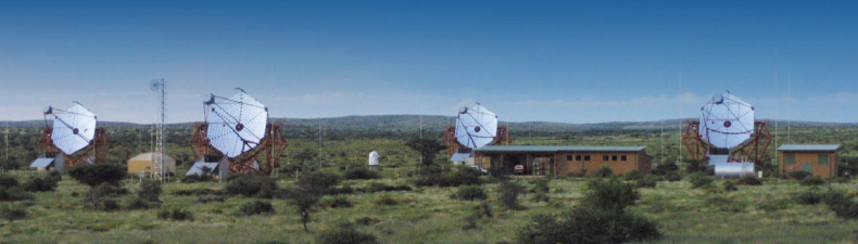
Figure 1.1: The H.E.S.S. array of four telescopes. Image credit www.unam.na/research/hess/

1.3 H.E.S.S. II phase

Recently (July 2012), a fifth telescope has been added to the array, what greatly enlarges the observatory capabilities. The 28 meter diameter telescope uses a parabolic-shaped mirror to minimize time dispersion. The dish is composed of 875 hexagonal faces of 90 cm size, with a focal length 36 m. The overall picture of the LCT is shown on figure 1.2.

The LCT camera follows the design of the H.E.S.S. I cameras, but is much larger. It is equipped with 2048 PMTs in 128 drawers. The physical pixel size is 42 mm, which is equivalent to a 0.067^∘ pixel FoV. The LCT pixels have the same physical size as of the SCT, but, due to the larger focal length, shower images are much better resolved.

The LCT is sensitive to photons down to 10 GeV. In the normal operations, any of the SCTs will be triggered only in case of a coincidence with another telescope (LCT or SCTs). Low energy photons will not trigger the SCTs. To increase the acceptance of low energy photons, standalone LCT triggers will have to be accepted.

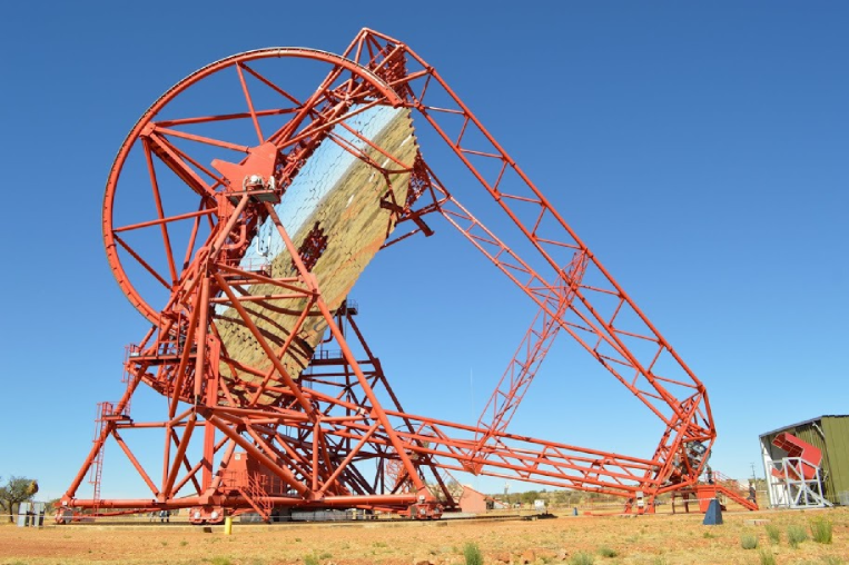
Figure 1.2: The overall picture of the large Cherenkov telescope of the H.E.S.S. array. Image taken during the H.E.S.S. II inauguration ceremony on 28 September 2012.

1.4 The principle of the Cherenkov technique

1.4.1 Cherenkov light emission

The Cherenkov light is emitted by a charged particle passing a dielectric medium with a velocity $v=\beta c$ greater than the phase velocity of light in that medium. The particle threshold velocity for the Cherenkov light production is:

$$\beta_{min}=\frac{1}{n},$$ (1.1)

where $n$ is a refraction index of the medium.

This can be translated into an energy threshold, $E_{th}$, for the particle:

$$E_{th}=\frac{m_{0}c^{2}}{\sqrt{1-\beta^{2}_{min}}}=\frac{m_{0}c^{2}}{\sqrt{1-n^{-2}}},$$ (1.2)

where $m_{0}$ is a particle rest mass.

Cherenkov photons are emitted with a fixed angle $\Theta$ to the particle trajectory. The angle can be calculated using the relation between the distance traveled by the particle and by the emitted radiation $t$ (see figure 1.3).

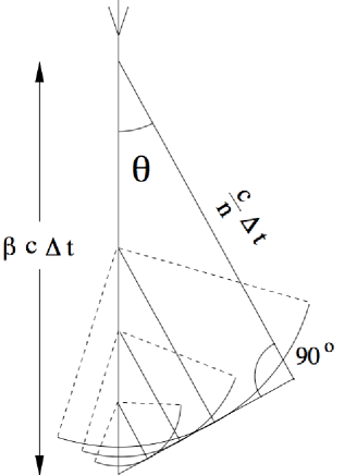
Figure 1.3: Cherenkov light wavefront.

$$\cos\Theta=\frac{(c/n)/t}{\beta ct}=\frac{1}{\beta n}.$$ (1.3)

In the case of IACTs, the relativistic particle o interest comes from the cascades initiated by cosmic rays (CR) particles in the Earth’s atmosphere.

1.4.2 Cosmic rays

Cosmic rays (CRs) are charged particles and atomic nuclei arriving at the Earth location from the all directions. They were discovered by the Austrian physicist Viktor Hess in a series of balloon experiments in the first decade of the XX^th century. Viktor Hess was awarded the Nobel prize in 1936 for this discovery. The CR spectrum is shown on figure 1.4. The spectrum, measured at the top of the Earth’s atmosphere, has the following composition: 98% of the particle are protons and nuclei, the remaining 2% are electrons. The protons and nuclei part is composed of 87% protons, 12% helium nuclei and 1% heavier nuclei.

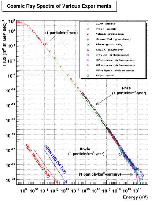
Figure 1.4: Differential cosmic ray particle flux spectrum as a function of energy. Figure shows the spectrum reported by different experiments. (Figure from http://www.physics.utah.edu/ whanlon/spectrum.html)

1.4.3 The atmospheric air showers

When the high energy CRs enter the Earth’s atmosphere, they collide with O₂ and N₂ molecules and produce new energetic particles. The generation of secondary particles starts at the height of about 20 km above the sea level, and continues until the depletion of the energy of the primary particle. The set of generated particles is called an atmospheric air shower. The showers initiated by hadronic or leptonic primary particles or photons have different compositions due to the nature of the physical processes involved.

Atmospheric showers caused by electrons or $\gamma$-ray photons develop as a pure electromagnetic cascades through electron positron pair production and bremsstrahlung radiation. When gamma rays interact with nuclei they produce $e^{\pm}$ pairs. In the next step, the electrons and positrons regenerate gamma rays by bremsstrahlung radiation.

The growth of hadronic cascade involves more types of possible interactions, thus results in the production of a greater variety of secondary particles like pions, kaons, nuclei, etc. The vast majority of the secondary particles produced after the first interaction are pions ($\pi^{+},\,\pi^{-},\,\,\pi^{0}$). The charged pions decay into muons $\mu$ and neutrinos $\nu$:

$$\pi^{\pm}\rightarrow\mu^{\pm}+\nu_{\mu}(\bar{\nu}_{\mu}).$$ (1.4)

The muons have a life-time of $\Gamma\times\tau_{\mu}$ with $\tau_{\mu}\sim 2.2\times 10^{-6}$ s and Lorentz factor $\Gamma$, which implies $c\Gamma\tau_{\mu}$= 1$\times\Gamma$ km. Therefore, they can travel through the atmosphere and reach the Earth’s surface. The Cherenkov light of such muons can trigger the cameras of IACT if muons reach the distance of a few hundred meters above the telescope. In such a case, typical arc shaped images or ring images are observed.

The neutral pions decay with 99% probability into photons $\gamma$:

$$\pi^{0}\rightarrow\gamma+\gamma,$$ (1.5)

and initiate a pure electromagnetic sub-shower.

In the case of electromagnetic showers, the vast majority of generated electrons is well collimated with the shower axis. This make the images of gamma showers very compact and regular. Hadronic showers are much less regular and less compact, because the nature of secondary particle is hadronic as well as leptonic, and the secondary particles are less collimated with respect to the shower axis. Figures 1.6 and 1.5 show two examples of the atmospheric air showers generated by the photon and proton, respectively.

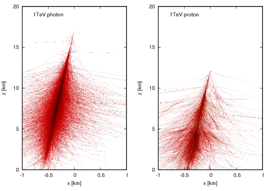
Figure 1.5: Two examples of extended air showers simulated with CORSIKA, developing in the Earth’s atmosphere. Each line represents a path of elementary particle created during shower evolution. The left panel presents the shower generated by a single photon of energy 1 TeV, while the right panel shows the shower originating from a single proton of the same energy.

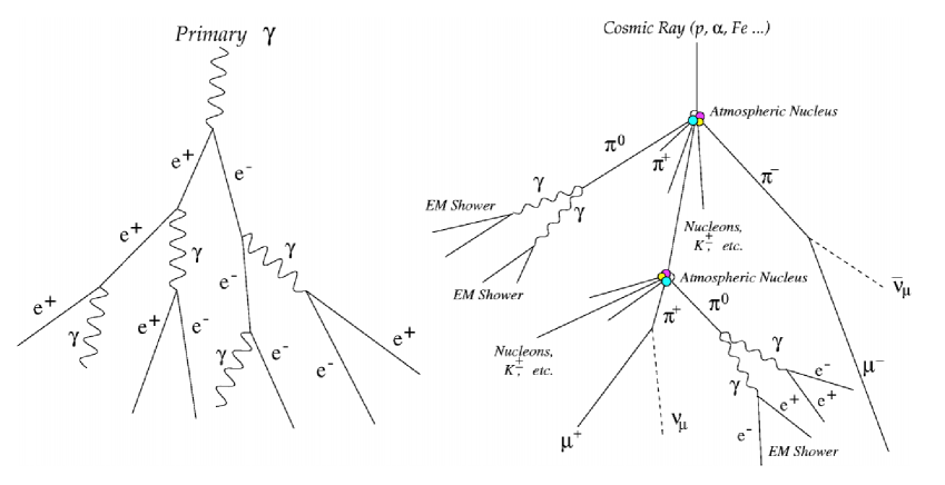
Figure 1.6: Schematic view of an electromagnetic (left) and a hadronic (right) air shower.

1.4.4 Air shower development in the atmosphere

In the electromagnetic cascade the number of secondary particles is nearly proportional to the energy, $E$, of the primary particle. After each radiation length $X_{r}$, the number of secondary particles increase by a factor of 2. After $n=X/X_{r}$ radiation lengths, the number of secondary particles is $N(X)=2^{X/X_{r}}$, where X is the slant depth along the shower axis (Gaisser, 1991).

The showers stop to develop when energy losses of secondary particles due to the pair production and bremsstrahlung emission are smaller than their losses by ionization. After this happens, secondary particles are absorbed by the atmosphere. The ionization energy loss, $E_{io}$, is about 2.2 MeV${\rm\,g^{-1}cm^{2}}$. The critical energy $E_{cr}$, below which the shower stops expanding is $E_{io}\times X_{r}$= 81 MeV, where radiation length $X_{r}$ in air is equal to 37 ${\rm g\,cm^{-2}}$.

The maximum number of particles in the shower, is reduced at the shower maximum $X_{MAX}$:

$$X_{MAX}=nX_{0}{\rm ln}(2)=X_{0}{\rm ln}\left(\frac{E}{E_{cr}}\right)\,.$$ (1.6)

The atmospheric depth, given in units of [${\rm g\,cm^{-2}}$], corresponds to an atmospheric heigh, $h$, in km:

$$X=X_{1}e^{-\frac{h}{h_{1}}}\,,$$ (1.7)

where $X_{1}=1013\,{\rm g\,cm^{-2}}$ and $h_{1}=8\,$km. Figure 1.7 shows the shower maximum height as a function of energy, assuming that the maximum of Cherenkov emission corresponds to the shower maximum $X_{MAX}$.

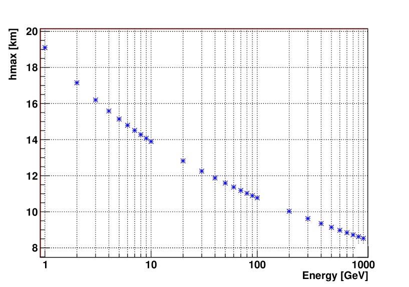
Figure 1.7: Shower maximum height as a function of primary particle energy.

1.4.5 Cherenkov light distribution

The number of Cherenkov photons per unit of track length of the particle and per unit of wavelength is given by the Frank-Tamm formula:

$$\frac{d^{2}N}{dl\,d\lambda}=\frac{2\pi\alpha Z^{2}}{\lambda^{2}}\sin^{2}\Theta=\frac{2\pi\alpha Z^{2}}{\lambda^{2}}\left(1-\frac{1}{\beta^{2}n^{2}(\lambda)}\right)\,,$$ (1.8)

where $\alpha=e^{2}/\hbar c$ is the fine structure constant, and $Z$ is the charge of the particle in units of the elementary charge. For atmospheric air showers the maximum intensity of the Cherenkov light emission corresponds to UV and blue light (300-700 nm). For shorter wavelengths it is cut off by the decrease of $n(\lambda)$. The cut off appears before X-rays because $n($X-rays$)<1$ in all materials. In addition, the Cherenkov light is strongly absorbed in the atmosphere before reaching the ground. The atmospheric absorption is more efficient toward the short wavelengths. This effect modifies significantly the observed spectrum. Figure 1.8 shows the spectrum of Cherenkov light emitted by a particle at 0^∘ zenith angle. The spectrum includes atmospheric absorption and for the comparison it is shown together with the quantum efficiency of PMT used by IACTs.

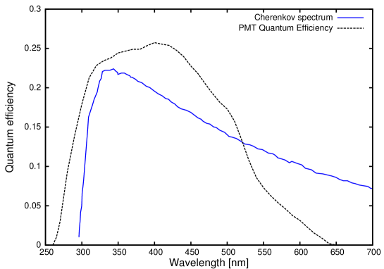
Figure 1.8: The blue line represents the Cherenkov light spectrum for a $0^{o}$ zenith angle detected at 2000 m above see level. The spectrum is shown after atmospheric absorption. The black dotted line shows the quantum efficiency of PMTs used in the H.E.S.S. camera.

The electromagnetic cascades of atmospherical showers are initiated at $\sim 22\pm 4$ km above the see level. Then, depending on the primary particle energy, the shower reaches its maximum between 15 km and 5 km. The charged secondary particles traversing the atmosphere emit Cherenkov photons with the cone angle $\Theta\sim 1^{\circ}$. Cherenkov photons emitted at 10 km produce a ring of radiation at the ground level with a radius of $\sim$120 m, centered on the particle trajectory. The shape of the ring depends also on the shower axis angle. The Cherenkov light distribution become more diffuse if the initial particle had a larger zenith angle.

The majority of Cherenkov photons, emitted between the first interaction and shower maximum, will arrive approximately within 120 m of the shower core. However, Cherenkov photons may have a significant flux many hundreds of meters from the shower axis. This is a consequence of the angular distribution of particles and the scattering of Cherenkov light.

Two examples of the Cherenkov light density distributions as a function of distance from the shower axis (impact parameter) are presented in figures 1.9 and 1.10, for $\gamma$-ray initiated showers and proton initiated showers, respectively. The distributions have been obtained using the CORSIKA package (Capdevielee et al., 1993). The light density of Cherenkov photons in the wavelength range 250-700 nm were simulated for gamma and proton showers. The magnetic field has been set in simulations for the H.E.S.S. site, and zenith angles $0^{\circ}$, azimuth angle $90^{\circ}$, and an altitude of 2000 m.

The Cherenkov light distribution of gamma showers shows a very regular structure with a characteristic bump at 120 m. The average photon density of proton showers is 3 times smaller than for the gamma showers of the same energy, since, on average only third part of energy of hadronic shower goes to electromagnetic sub-showers.

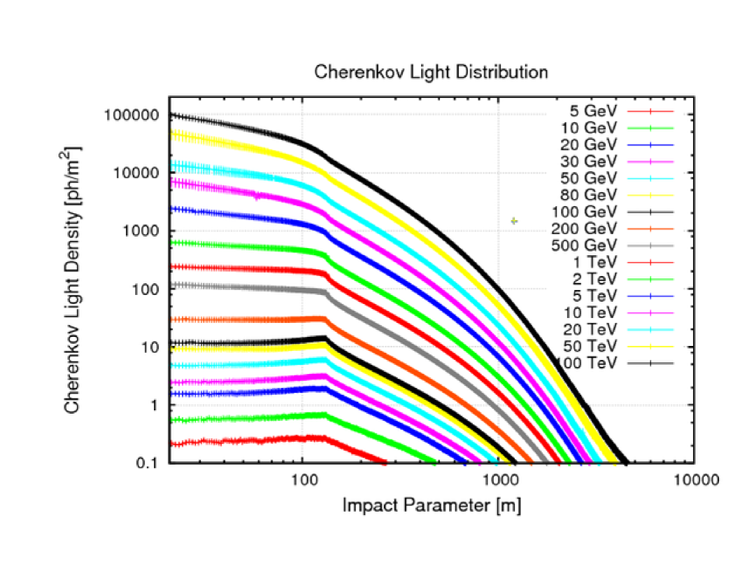
Figure 1.9: Cherenkov light distribution: $\gamma$-ray initiated showers.

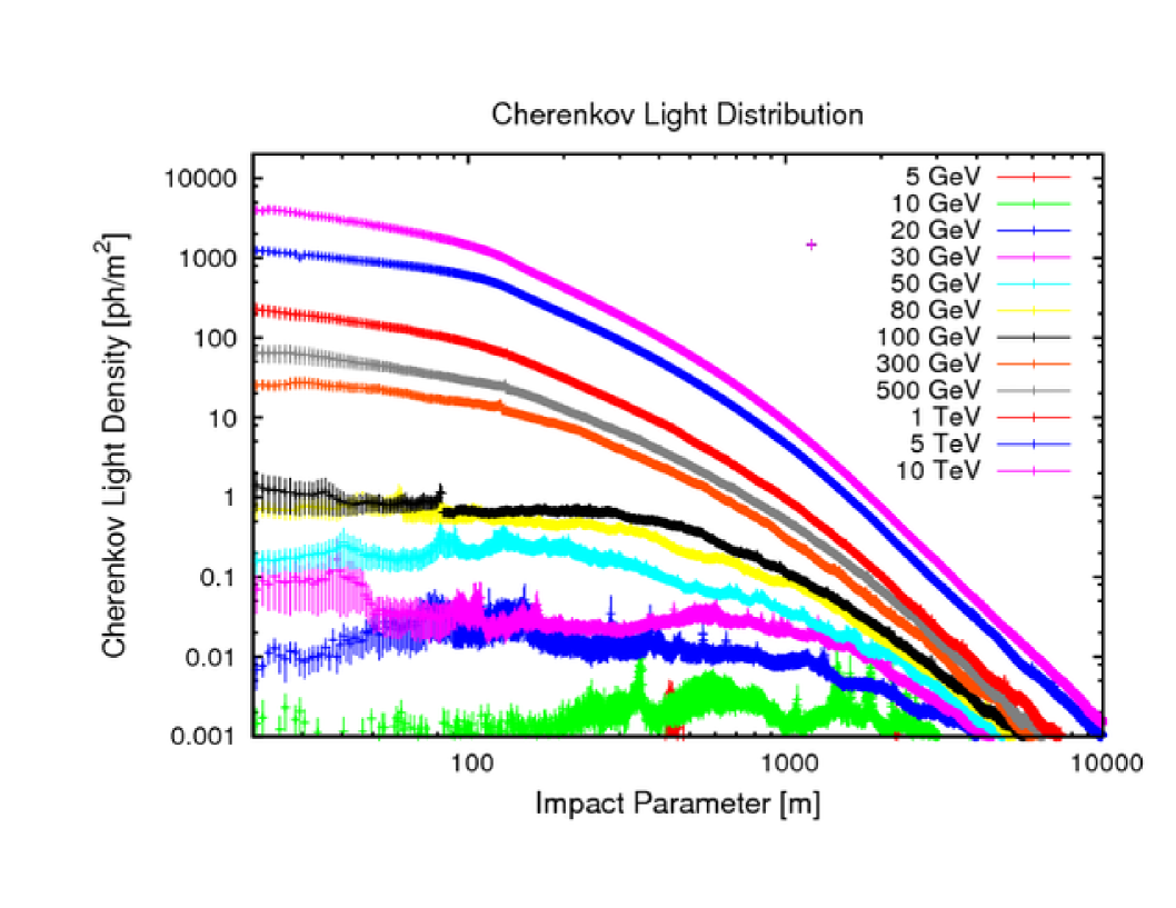
Figure 1.10: Cherenkov light distribution: proton initiated showers.

1.4.6 Shower geometry

The Cherenkov light emitted by the atmospheric shower is observed in the focal plane of ground based instruments. The image of gamma showers in the camera has an elliptical shape which can be characterized by Hillas parameters (Hillas, 1985). The Hillas parameters are obtained by calculating moments of the photo-electron (phe) distribution in the camera. The most comonly used parameters in the image analysis are Size, Length, Width, Alpha and Dist. These parameters are shown on figure 1.12.

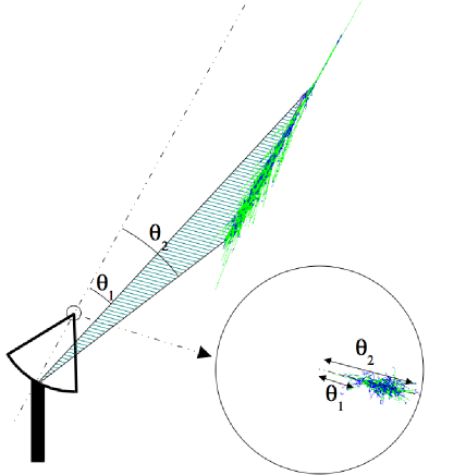
Figure 1.11: The principle of the Cherenkov imaging technique (Guy, 2003).

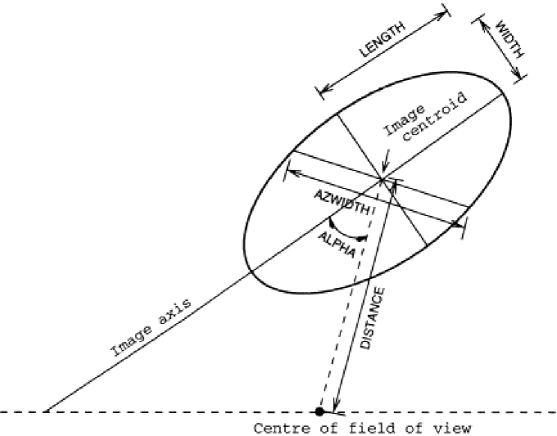
Figure 1.12: The elliptical contour of a typical Cherenkov light image as seen in the focal plane of camera of IACTs.

The Size parameter is the total number of photo-electrons in the image and is roughly proportional to the energy of the primary particle, it is also called the Amplitude. The second moment of the phe distribution with substracted COG (the image center of gravity) along the major image axis is the Length, and along the minor axis is the Width. The Alpha is the angle between the direction of the major axis and the line joining the image centroid with the source position.

The Dist is the distance between the image centroid and the source position in the camera plane. The Dist parameter is correlated with the distance of the shower to the telescope axis (impact parameter). The correlation between Dist and impact parameter (IP) is presented in figure 1.13. The correlation is energy dependent because the image maximum for different energies of primary particle appears at different heights (see figure 1.13). The relation between the energy and shower maximum height has been calculated from equations (1.6) and (1.7).

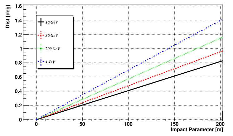
Figure 1.13: Dist parameter as a function of the impact parameter for different energies of the primary gamma photon.

1.5 Analytical estimation of the energy threshold of the H.E.S.S. LCT

The theoretical energy threshold of the H.E.S.S. telescope can be calculated using the Cherenkov light distribution and the overall performance parameters of the telescope. The minimum photon density, $\rho_{ph}$, required to obtain the signal of at least $N_{phe}$ is defined as:

$$\rho_{ph}=\frac{N_{phe}}{(A-A_{C})\times R\times QE}$$ (1.9)

where $A$ is a mirror effective area, $A_{C}$ is the camera and masts shadowing, $R$ is system reflectivity, $QE$ is integrated detector efficiency weighted by the Cherenkov light spectrum.

	H.E.S.S. SCT	H.E.S.S. LCT
Mirror effective area $A[$m${}^{2}]$	113	600
Camera shadowing $A_{C}[$m${}^{2}]$	1	1
System reflectivity $R$	0.8	0.8
Average photodetector QE	0.1	0.1

Table 1.1: The parameters of the H.E.S.S. telescopes.

Typically 50 – 100 phe are necessary to perform an image reconstruction. Using equation (1.9) and the telescope specifications listed in table 1.1, one can derive the photon density required to detect certain number of photo-electrons. For the H.E.S.S. I telescopes, a density of $\sim$5.5–11$\,{\rm ph\,m^{-2}}$ is required to detect 50 – 100 photo-electrons. This density corresponds to an energy of 60 – 100 GeV, according to figure 1.9. This is the energy threshold of the H.E.S.S. I detector.

The H.E.S.S. II telescope has a reflection area more than 5 times larger than the H.E.S.S. I telescopes. This allows to collect enough photons from a much smaller signal. In the case of the H.E.S.S. II, a minimum photon density of $\sim$1–2 ${\rm ph\,m^{-2}}$ is required to detect 50 – 100 photo-electrons. This photon density correspond to gamma shower energies of 10 – 20 GeV.

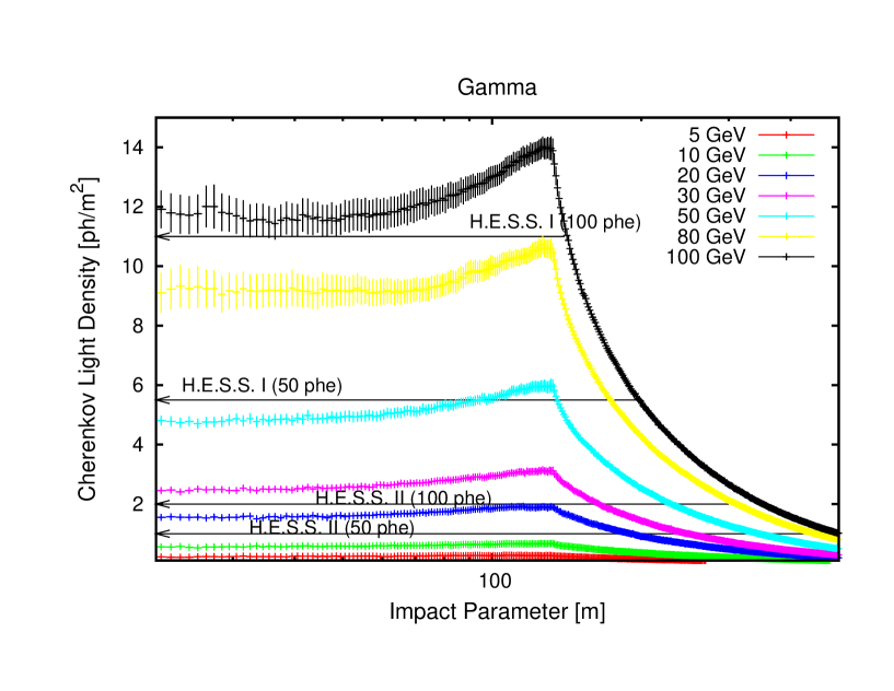
Figure 1.14: Cherenkov light distribution for low energy gamma showers. The arrows indicate the minimum photon density required to detect 50 – 100 phe by the H.E.S.S. I and the H.E.S.S. II systems.

The numbers quoted above refers to the trigger threshold, and are estimated for observations at zenith angle $0^{o}$. The numbers give a rough estimate of the system performances. The LCT will work alone in the energy range from 10 GeV to 60 GeV. The telescopes should work efficiently together in stereoscopic mode for energies above 60 GeV. In the case of observations at larger zenith angle, the energy threshold for the stereoscopic trigger is larger.

1.6 Trigger system of the H.E.S.S. II telescope

The trigger system of the H.E.S.S. II will operate at three levels: the Level 1 trigger (camera level), the Level 2 trigger (LCT level) and the stereoscopy (array level). In addition to time coincidences between SCT Level 1 triggers, the central trigger system will check for time coincidences of LCT and SCTs triggers. The result of the latter coincidence test (monoscopic or stereoscopic event) will be sent back to the LCT trigger management. As in H.E.S.S. I, stereoscopic events will always be accepted.

1.6.1 Level 1 trigger

The LCT has a Level 1 trigger similar to the Level 1 trigger of the four small telescopes. It is a local camera trigger described in details by Funk et al. (2005). A camera Level 1 trigger occurs if the signals in M pixels (pixel multiplicity) of a camera sector, exceed a threshold of N photoelectrons (pixel threshold). Each sector consists of 64 pixels. The LCT camera was divided to 96 overlapping sectors to ensure trigger homogeneity. The effective time window for coincidence is 1.3 ns.

1.6.2 Level 2 trigger

The small Cherenkov telescopes are not equipped with a Level 2 trigger, since they do not operate in mono mode. The LCT was build to lower the energy threshold of triggered gamma events. Normally, the background rejection is achieved in the stereoscopic mode when more than one small telescope is triggered at the same time as the large telescope. The stereoscopy with the large telescope will allow to lower the energy threshold down to 50 – 60 GeV (as was discussed in section 1.5). The LCT has to work in mono mode below this energy range. The mono mode does suffer from high trigger rates caused by single muons. The solution with Level 2 trigger has been proposed for LCT to reduce the trigger rate.

1.6.3 Stereoscopy

The step after the camera trigger level (Level 1 trigger) is the so-called central trigger. The central trigger system looks for coincidences of telescope triggers inside a 40 ns time window. A coincidence of at least 2 telescopes is required in the central trigger time window. LCT monoscopic events are accepted or rejected depending on the result of Level 2 system evaluation. The possible configurations of stereoscopy are shown on figures 1.15 and 1.16.

Figure 1.15: The array of 4 telescopes requires a coincidence of at least two SCTs. Red color indicates not triggered telescope, white green color indicates triggered telescope.

Figure 1.16: The configuration of the full array (4 SCT + 1 LCT) required to fire the central trigger. Red color indicates not triggered telescope, white green color indicates triggered telescope.

1.7 Algorithms for the Level 2 trigger

1.7.1 Requirements for the Level 2 trigger

The input rate to the Level 2 trigger is limited to less than roughly 100 kHz by the dead-time of the front-end readout board. In turn, the output rate is limited to a few kHz by the capacity of the ethernet connection to the acquisition system.

Table 1.2 shows the trigger rates caused by the NSB for different pixel multiplicities and thresholds. The input rate gives a strong constraint on possible Level 1 trigger conditions: pixel multiplicity and pixel threshold. The total particle and NSB rate is at the level of a few kHz. A further reduction of this rate by a factor of 2 or 3 allows to fulfill the output rate condition even in very noisy environments.

1.7.2 Principle of the Level 2 trigger

The idea of the Level 2 trigger is to have the whole trigger information at the pixel level, instead of the sector level as in the Level 1 trigger. A reduced, 3-level image of the camera, so-called “combined map”, is sent to the Level 2 trigger system whenever the LCT has an confirmation of Level 1 trigger.

The combined map consists of two black and white images of the camera, with 3 possible pixel intensities, which are 0 (when a pixel is below the threshold), the Level 1 pixel threshold and another higher pixel threshold. The black and white image obtained by taking only the Level 1 threshold information (resp. the Level 2 threshold information) is called “Level 1 map” (resp. “Level 2 map”).

The background rejection is performed by a dedicated algorithm, described in detail in subsections 1.7.4 or 1.7.5. Since stereoscopic events should always be accepted, the Level 2 trigger operates differently on stereoscopic and monoscopic events. When the Level 1 trigger of the LCT occurs, the central trigger checks, if another telescope was triggered. If this is the case, then the event is accepted by the Level 2 system. If on the contrary the event is monoscopic, the decision depends on the Level 2 trigger algorithm.

1.7.3 Approach to the algorithm

For monoscopic events the trigger rate can be reduced with a two step procedure. The first step rejects NSB events, which have been accepted by Level 1 system in the procedure called clustering/denoising. The second step lowers the rate caused by the particle background events (protons, muons, electrons), through the topological algorithms. The crucial requirement is to keep as many gamma events as possible during each of the above steps.

1.7.4 Clustering/denoising

The NSB consist of photons from stars and a diffuse light. Therefore, no correlation is expected between the pixels illuminated by NSB. These events can be rejected requiring pixels with signals above the pixel threshold from a cluster of neighboring pixels, the so-called ”clustering” condition. Most of the pixels fired by NSB photons are isolated, and they can be removed by a step called ”denoising”.

The denoising algorithm removes all the isolated pixels from the Level 1 map. If the resultant map is empty then the event is rejected. There are several possible clustering algorithms. One variant simply demands a group of 2 or 3 neighboring pixels above a trigger threshold. The effect of the denoising/clustering on the trigger rate cased by NSB for a cluster of at least 2 pixels above the threshold is illustrated in table 1.2. The NSB trigger rates decrease by large factors, in some cases by several order of magnitude (see e.g. the trigger rates in table 1.2 for a pixel threshold of 3 photoelectrons and multiplicity of 3 pixels). The efficiency of the clustering/denoising algorithm allows to decrease the Level 1 trigger threshold and thus to reach a smaller photon energy threshold.

Protons, electrons, and total particle rates as a function of trigger condition are displayed on figures 1.19, 1.21 and 1.22, respectively. These rates are little affected by the clustering cut. The electron rate is dominated by low energy events, so that most electron events will trigger only the LCT.

1.7.5 Topological algorithms

The topological algorithms rely on the fact that the images of showers observed in the camera plane have a characteristic shape. The images of gamma-like events are well defined by the Hillas parameters described in section 1.4.6. The images created by hadrons have much less regular shape, and thus Hillas parameters can be used to separate the electromagnetic from hadron-like showers. The single muons created in the hadronic cascade produce a very characteristic ring or arc shapes.

Therefore, it is worth investigating, which of the Hillas parameters can be used in the trigger to reject hadron like events, without losing too many gamma events. The time duration of the shower depends on the primary particle energy and the impact parameter. The shower event on the ground can lasts from a few to dozen of ns in the case of very energetic events. The maps processed by the Level 2 trigger contain the signal integrated in $\sim$ 1 ns, so it contains only a fraction of the shower image.

Figures 1.17 and 1.18 show shower parameters (Width, Length, Amplitude, COG, Length/Size, Width/Length) computed for the signal integrated over 16 ns compared to the one calculated from 1 ns Level 2 combined maps. The comparison is presented for 30 GeV and 100 GeV simulated gamma showers. The figures show barely any correlation for the Width and Length parameters, but there are strong correlations for the COG and the Amplitude parameters. Therefore, the COG or the Amplitude cuts can be used to further reduce the hadron rate.

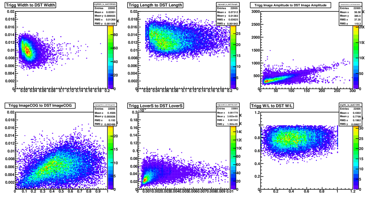
Figure 1.17: Comparison of the showers parameters calculated using the Level 2 maps and the processed images after cleaning (DST). The comparison has been performed for 30 GeV gamma showers. The Hillas parameters have been calculated using a 1/3 image cleaning.

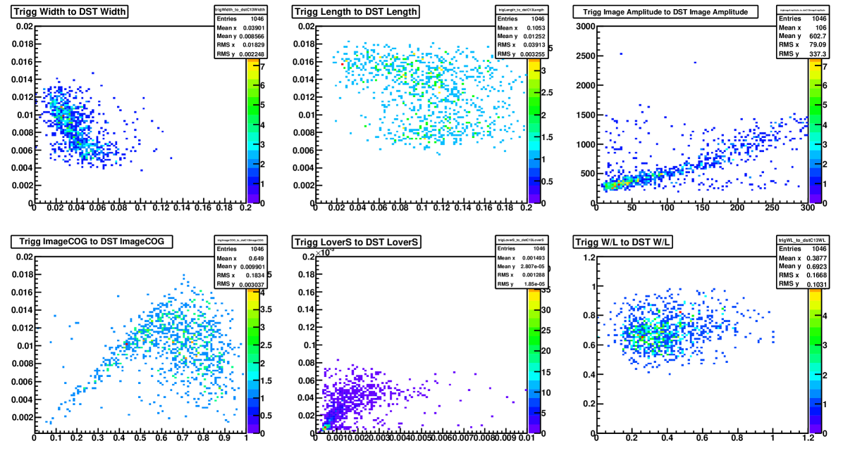
Figure 1.18: Comparison of the showers parameters calculated using the Level 2 maps and the processed images after cleaning (DST). The comparison has been performed for 100 GeV gamma showers. The Hillas parameters have been calculated using the H.E.S.S. DST with a 1/3 image cleaning.

1.7.6 The center of gravity cut

The algorithm that can be used to reject a part of the background particles is based on the center of gravity (COG) cut. The COG parameter was chosen, because for low energy gamma showers, the COG shows a clear correlation between the one calculated from instantaneous Level 2 maps and that calculated from the whole image integrated over 16 ns.

The other reason for using the COG parameter comes from the shower geometry. The LCT is design to detect low energy gamma events. The showers initiated in the atmosphere by low energy $\gamma$-ray photons have their maximum higher in the atmosphere (see. figure 1.7). The Cherenkov light distribution at low energy (figure 1.14) shows that low energy gammas have a photon density large enough to be detected up to $\sim$ 200 m. The lateral distribution reaches its maximum at $\sim$120 m, and then decreases rapidly. Figure 1.13 shows the DIST parameter as a function of the impact parameter calculated for different energy of primary gammas. From figure 1.13 its clear that at low energies ($\sim 10-30$ GeV) the majority of showers will have their COG positions within 1^∘ radius from the source position. We thus demand that the COG of accepted showers be located at less than $1.75^{\circ}/\sqrt{3}=1^{\circ}$ from the expected position of the source.

The higher energy $\gamma$-rays produce air showers with enough Cherenkov photons to trigger more than one telescope. Thus they will be accepted by the stereoscopic trigger. This algorithm is valid for point sources or weakly extended sources of photons.

The direction of the charged primary particle is changed by the Galactic and the Earth magnetic field. The observed distribution of the background events is then isotropic. The COG of such particles are uniformly distributed in the focal plane of the telescope. The fraction of the background events rejected with the COG cut is proportional to the excluded area. The COG cut set at 1^∘ should reject 1 – COG${}_{cut}^{2}/(\mbox{FoV}/2)^{2}\approx$ 70% of the background events.

1.8 Trigger simulations

The trigger simulations have been performed using KASKADE and SMASH tools. KASCADE (Kertzman & Sembroski, 1994) package is a computer software that simulates in three dimensions the Cherenkov photons produced by VHE gamma-rays and hadronic air showers.

SMASH is a package dedicated to the H.E.S.S. detector simulation. The package is used to simulate the response of the detector to the Monte Carlo photon data produced with KASCADE.

SMASH reproduces the camera, dish and telescope structure geometry. The package simulates the whole electronics as well as the background and noise contributions. The different Level 2 schemes have been implemented by the author to the SMASH software. The electronic channel outputs were simulated with realistic photon signal shapes and a realistic electronics readout. The results of the simulations have been used to estimate the various trigger rates with the method described by Guy (2003).

1.8.1 Background rates

The largest contributions to the trigger rate of a single telescope in $\gamma$-ray astronomy are background events. The largest fraction of the events triggering the camera are photons from the NSB. The other major source of background are cosmic ray showers. These showers have either hadron (proton, helium, etc.) or electron/positron primaries. The typical proton flux is larger than 100 particles m^-2sr^-1s^-1 taking into account protons with energies above 10 GeV. The expected muon flux is about $\sim$10 particles m^-2sr^-1s^-1, while the electron flux above 7 GeV is $\sim$3 particles m^-2sr^-1s^-1. The background rates are calculated according to the formula:

$$\mbox{Background\,rate}=\frac{N_{trigg}}{N_{sim}}\times\Omega\times S\times\int_{E_{min}}^{E_{nax}}\frac{dN}{dE}$$ (1.10)

where $\Omega=2\pi[1-\cos(\mbox{viewcone})]$ is the solid angle of the viewcone in steradians, $S=\pi\times IP_{max}^{2}$ is the area with radius which corresponds to the maximum impact parameter $IP_{max}$, of simulated events. $N_{trigg}$ is a number of triggered events and $N_{sim}$ is a number of simulated events. The particle flux, $dN/dE$, is known from observations of many instruments and differ for each particle type.

1.8.2 Proton rate

Protons were simulated in the energy range from 0.005 TeV to 500 TeV, with the maximum impact parameter of 550 m and the viewcone of 5^∘. The proton trigger rates were calculated using the particle flux given by Guy (2003) [Chapter 13, p.135] and using equation (1.10):

$$\frac{dN}{dE}=1.49\times 10^{4}(E+2.15e^{-0.21\sqrt{E}})^{-2.74}{\rm m^{-2}s^{-1}sr^{-1}GeV^{-1}}.$$ (1.11)

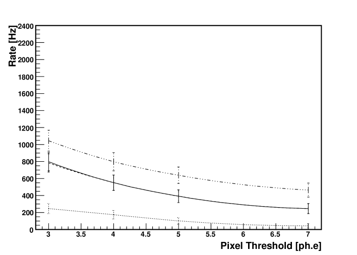
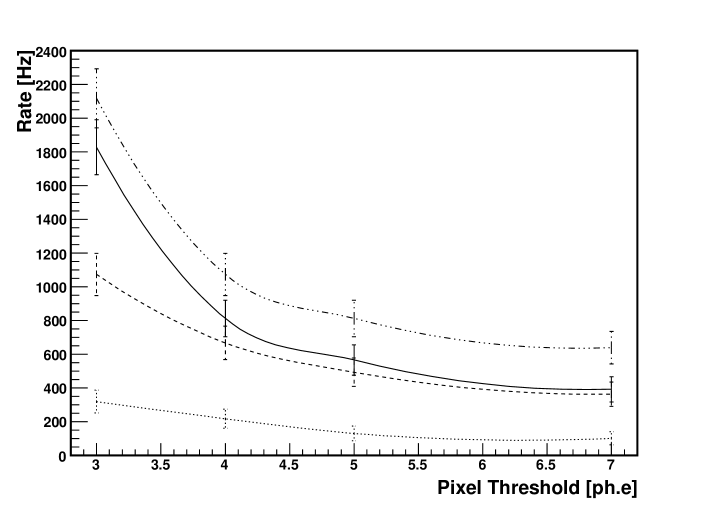
Figure 1.19: Proton trigger rate versus pixel threshold (in photoelectrons). On the top figure the pixel multiplicity is 4 and on the bottom figure is 3. A Level 2 pixel threshold of 7 have been assumed. The dash-dotted line gives the raw level 1 rate. The solid line shows the rate of monoscopic events. The dashed line gives the rate of events passing the cleaning/denoising pixel cut. Finally, the dotted line is the rate of events passing the COG cut. Note that the COG cut reduces the proton rate by a factor of 3.

The proton trigger rate is shown on figure 1.19 as a function of the pixel threshold in photoelectrons.

1.8.3 Muon rate

Isolated muons from distant hadronic showers can trigger Cherenkov telescopes. These muon triggers dominate the single telescope triggers (Funk et al., 2005) and can be rejected by demanding a multi-telescope trigger (stereoscopy). The muons flux were calculated using:

$$\frac{dN}{dE}=431E^{-2.3}e^{-0.38/E}(1-e^{\frac{-33}{E}}){\rm m^{-2}s^{-1}sr^{-1}GeV^{-1}}\,.$$ (1.12)

The energy range of simulated muons was 10 – 100 GeV. The trigger rate contributed by single muons is shown on figure 1.20.

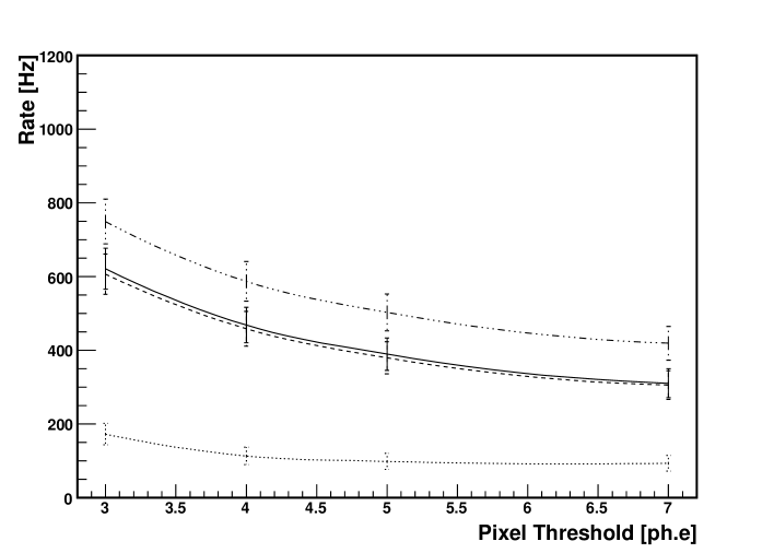
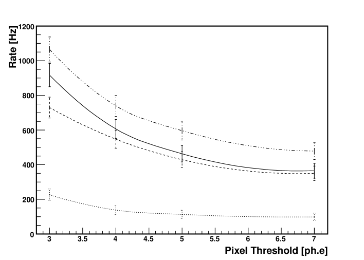
Figure 1.20: Part of the trigger rate due to the isolated muon component of the shower. Level 1 pixel multiplicity of 4 (top figure) and 3 (bottom figure), and Level 2 pixel threshold of 7 have been assumed. The dash-dotted line gives the raw Level 1 rate. The solid line shows the rate of monoscopic events. The dashed line gives the rate of events passing the cleaning/denoising pixel cut. Finally, the dotted line is the rate of events passing the COG cut. Note that the COG cut reduces the single muon rate by a factor of 3.

1.8.4 Electron rate

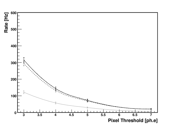
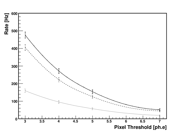
Figure 1.21: Electron rate as a function of the pixel threshold. Level 1 pixel multiplicity of 4 (top panel) and 3 (bottom panel), and Level 2 pixel threshold of 7 have been assumed. The dash-dotted line gives the raw Level 1 rate. The solid line shows the rate of monoscopic events. These 2 lines are almost superimposed since the electron rate is dominated by low energy events. The dashed line gives the rate of events passing the cleaning/denoising pixel cut. Finally, the dotted line is the rate of events passing the COG cut.

Cosmic ray electrons give a Cherenkov signal very similar to the signal of high energy gamma rays. It is thus not possible to eliminate electrons from the analysis. However, the electron background, which is a diffuse source, can be reduced in point source studies. The trigger rates were calculated using the particle flux:

$$\frac{dN}{dE}=0.95\times 10^{-4}\left(\frac{E}{1TeV}\right)^{-3.26}{\rm m^{-2}s^{-1}sr^{-1}TeV^{-1}}.$$ (1.13)

The minimum energy of electron entering the atmosphere depends on the rigidity cut-off (Cortina & González, 2001). The geomagnetic field bends the cosmic ray trajectories preventing low rigidity particles from reaching the Earth’s surface. The rigidity of a particle is defined as $pc/Z$, where $c$ is the speed of light, $p$ is the particle momentum and $Z$ is the charge of the particle. The minimum allowed rigidity is known as rigidity cut-off, $R_{c}$. The electron rigidity cut-off can by estimated from

$$R_{c}=\frac{59.4\cos^{4}\lambda}{r^{2}(1+\sqrt{1-cos^{3}\lambda\sin\theta\sin\phi})^{2}}\,,$$ (1.14)

where:
$\theta$ - is the zenith angle ($\theta=0^{o})$
$\phi$ - is the azimuth angle ($\phi=90^{o})$
r - is the distance from the dipole center
$\lambda$ - is the magnetic altitude
A simple manipulation of the rigidity definition gives an expression for the minimum energy of the particle which are able to penetrate into the Earth’s atmosphere:

$$E_{min}=\sqrt{(Z\,R_{c})^{2}+m_{0}^{2}c^{4}}\,.$$ (1.15)

For the H.E.S.S. site, the geographic longitude is 18^∘ E, the geographic latitude 22^∘ S, and the corrected magnetic latitude is 33^∘. The rigidity cut-off for H.E.S.S. site is then $R_{c}$=7 GV. The cut-off energy for the electrons is thus $E_{min}\simeq 7$ GeV.

Monte Carlo samples of cosmic electrons were simulated using the following parameters: energy range from 0.007 TeV to 300 TeV, viewcone 5^∘. The electron trigger rate is typically a few hundred Hz, and is plotted on figure 1.21.

1.8.5 Total particle trigger rate

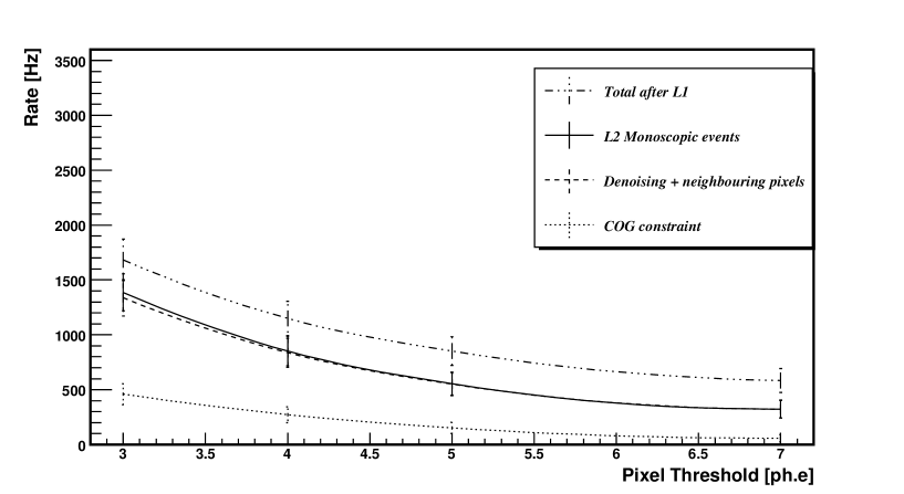
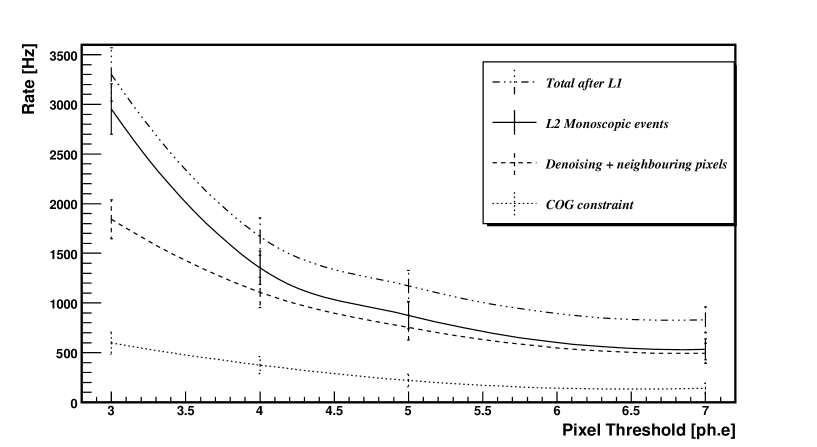
Figure 1.22: Total hadronic+electron rate as function of the pixel threshold. Level 1 pixel multiplicity is 4 (top panel) and 3 (bottom panel). Level 2 pixel threshold of 7 have been assumed. The dash-dotted line gives the raw Level 1 rate. The solid line shows the rate of monoscopic events. The dashed line gives the rate of events passing the cleaning/neighbouring pixel cut. Finally, the dotted line is the rate of events passing the COG cut.

The particle trigger rate is shown as a function of the pixel threshold on figure 1.22. The particle trigger rate is the sum of the proton, the helium and the electron rate. The helium rate is taken into account by multiplying the proton rate by 1.2 (Guy, 2003). The total particle trigger rate is of the order of 1 kHz.

1.8.6 Night Sky Background rate

The NSB comes from diffuse sources, such as the zodiacal light and the galactic plane, and light from bright stars. The NSB flux has been measured at the H.E.S.S. site and NSB photoelectron rates were derived for the 12 meter telescopes (Preu et al., 2002). The calculated NSB photoelectron rate is $100\pm 13$ MHz per pixel at zenith in extragalactic fields. In galactic fields, the single pixel rate is higher and reaches 200-300 MHz per pixel. The 28 meter telescope has a larger collection area (596 m² as compared to 108 m²), but with more pixels (2048 instead of 960) and a smaller angular acceptance ($3\times 10^{-3}$ sr instead of $6\times 10^{-3}$ sr), the expected NSB rate per pixel of the LCT is only a factor of 1.3 higher as compared to SCT.

KASKADE simulations have been used to generate gamma particles with very low energies not producing detectable Cherenkov light to reproduce the response of the detector to the NSB events. The gamma energy has been set arbitrarily to $5\,$MeV. The NSB trigger was then simulated by adding random photoelectrons to every readout channel. NSB single pixel rates of 100, 200 and 300 MHz were studied. The different NSB levels have been set to reproduce different observation conditions. The low NSB level $\sim$ 100 MHz is relevant for an extragalactic observation. The high NSB level $\sim$ 300 MHz corresponds to the photon background for the Galactic plane observations.

The NSB rate has been calculated by looking for a trigger in a 40 ns coincidence window:

$$\mbox{NSB\,rate}=\frac{N_{trigg}}{N_{sim}}\times\mbox{Window\, Duration}\,.$$ (1.16)

The LCT trigger rates due to the NSB are shown on table 1.2 for several Level 1 trigger conditions. Depending on the conditions, the estimated rates range from several MHz to less than a few tens of Hz. Since the dead-time per event of the LCT acquisition is of the order of a few microseconds, the acquisition rate should be less than roughly 100 kHz. Table 1.2 shows that some Level 1 trigger condition (e.g. a pixel multiplicity of 3 and a pixel threshold of 3) lead to unmanageably high trigger rates.

(Multiplicity,	L1 rate	L1 rate	L1 rate
Pixel Threshold)	100 MHz	200 MHz	300 MHz
(4,3)	$<$ 63 Hz	655 $\pm$ 182 Hz	183 $\pm$ 3.6 kHz
(4,4)	$<$ 63 Hz	$<$ 120 Hz	142 $\pm$ 51 Hz
(4,5)	$<$ 63 Hz	$<$ 120 Hz	$<$ 160 Hz
(4,5)	$<$ 63 Hz	$<$ 120 Hz	$<$ 162 Hz
(3,3)	803 $\pm$ 80 Hz	125 $\pm$ 2.3 kHz	7 $\pm$ 0.18 MHz
(3,4)	84 $\pm$ 40 Hz	1 $\pm$ 0.2 kHz	16 $\pm$ 1 kHz
(3,5)	21 $\pm$ 20 Hz	63 $\pm$ 37 Hz	1 $\pm$ 0.3 kHz
(3,7)	$<$ 63 Hz	$<$ 120 Hz	320 $\pm$ 156 Hz

(Multiplicity,	clustering	clustering	clustering
Pixel Threshold)	100 MHz	200MHz	300 MHz
(4,3)	$<$ 63 Hz	230 $\pm$ 112 Hz	171 $\pm$ 3.5 kHz
(4,4)	$<$ 63 Hz	$<$ 120 Hz	$<$ 160 Hz
(4,5)	$<$ 63 Hz	$<$ 120 Hz	$<$ 160 Hz
(4,5)	$<$ 63 Hz	$<$ 120 Hz	$<$ 160 Hz
(3,3)	$<$ 63 Hz	13 $\pm$ 0.24 kHz	8.7 $\pm$ 0.17 kHz
(3,4)	$<$ 63 Hz	$<$ 120 Hz	510 $\pm$ 212
(3,5)	$<$ 63 Hz	$<$ 120 Hz	$<$ 160 Hz
(3,7)	$<$ 63 Hz	$<$ 120 Hz	$<$ 160 Hz

Table 1.2: Night sky background rates for NSB levels of 100 MHz, 200 MHz and 300 MHz. Upper limits are given at the 95% C.L. Upper table: Night Sky Background rates for various trigger conditions. Lower table: effect of denoising and clustering. The clustering condition asks for at least 2 neighbors around at least one triggered pixel.

1.8.7 Effective area

The advantage of the Cherenkov imaging technique is its large collection area. The gamma efficiency (number of triggered events divided by number of simulated events) alone does not gives even a rough estimate of the telescope performance. To check the performance more accurately it is much better to calculate the effective area, which include also the information about the trigger efficiency as a function of the impact parameter. The effective collection area, $A_{{\rm eff},\gamma}$, of a single telescope is determined by the lateral and angular distribution of the Cherenkov light. For gamma-rays from a point source:

$$A_{{\rm eff},\gamma}(E)=2\pi\int_{0}^{\infty}P_{\gamma}(E,r)r{\rm d}r\,,$$ (1.17)

where $P_{g}(E,r)$ is the detection probability for a gamma-ray shower induced by a primary photon with energy E and impact parameter r.

Figure 1.23 shows the detection probability as a function of the impact parameter for 20 GeV gamma showers at different trigger conditions. It is worth pointing out that at low energy the trigger efficiency depends very strongly on the Level 1 trigger conditions. However, at very low trigger thresholds the trigger efficiency is increased by random NSB hints. The simulations of gamma showers has been performed with additional photon noise at level of 100 MHz. Figure 1.24 shows the comparison of effective areas at different trigger conditions and trigger algorithm stages.

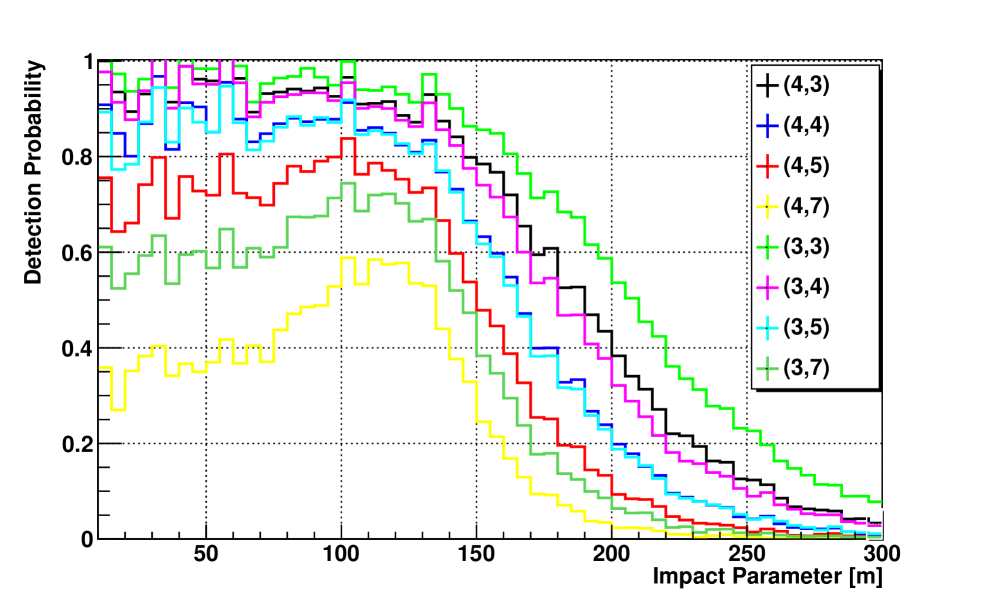
Figure 1.23: The detection probability as a function of impact parameters for gamma showers of energy 20 GeV. The legend indicate the Level 1 trigger condition (multiplicity and pixel threshold). The gamma detection probability is presented for events accepted by the Level 1 trigger.

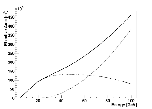
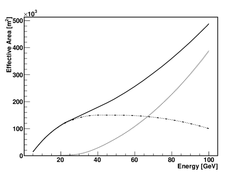
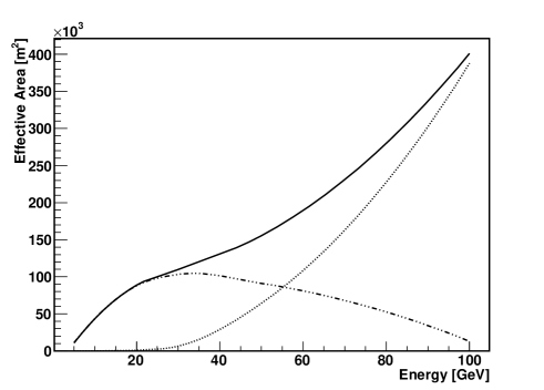
Figure 1.24: The effective area calculated for Level 1 trigger multiplicity 3 (up panel) and 4 (down panel). The effective area is presented at two different stages of the trigger. The left panel shows the effective are after Level 1 trigger and the right panel the effective area after COG cut. The dashed dotted lines indicate the effective area of monoscopic events. The dotted lines indicate the stereoscopic events. The solid line is the sum of monoscopic and stereoscopic events.

1.8.8 Level 2 trigger efficiency

The efficiency of the different algorithm steps has been tested with the Monte Carlo simulations. Figure 1.25 shows the results of the simulations for each step of the algorithm. The solid line indicate the total efficiency of the algorithm as a function of $\gamma$-ray event energies. At energies below 30 GeV all events are monoscopic (the dot-dashed line). Above 30 GeV, a small fraction of the events start to be stereoscopic, then stereoscopy is starting to be efficient above an energy of 60 GeV. All stereoscopic events are accepted. The fraction of the stereoscopic events is represented by the area above the dot-dashed line.

The algorithm based on the COG cut is very efficient at low energies (the dotted line). At higher energies the stereoscopy is starting to work very efficiently and the majority of gamma events are thus accepted. The solid line indicate that for energies below 40 GeV the efficiency of the algorithm for accepting gamma events reach 80%.

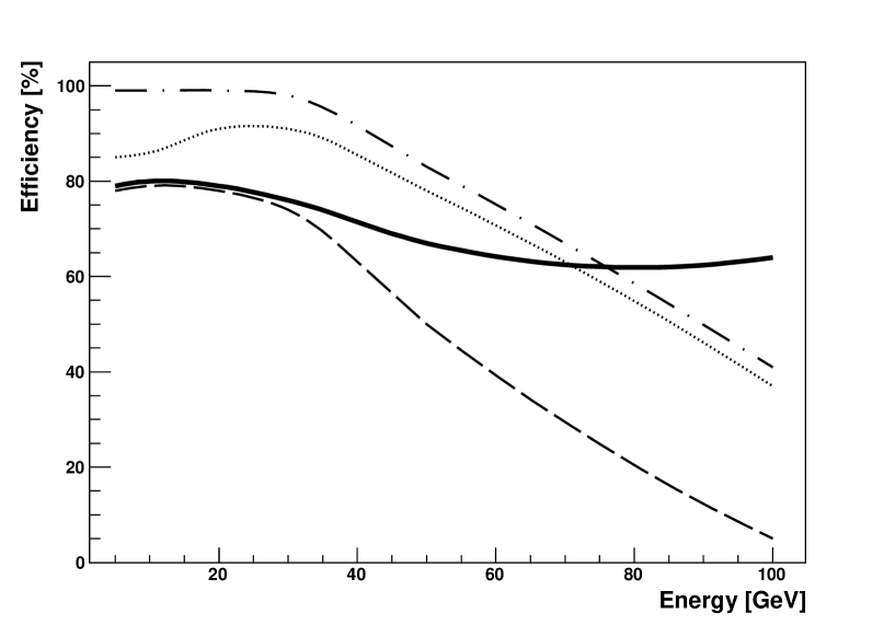
Figure 1.25: Level 2 trigger efficiency as a function of shower energy in the case of filtering by the simple COG algorithm described in the text. The efficiency is normalized to the Level 1 trigger photon efficiency. The dot-dashed line shows the fraction of monoscopic events. The dotted line and the dashed line show respectively the effect of the clustering/denoising algorithm and the combined effect of the nearest neighbor and COG algorithms. The Level 2 trigger efficiency is the sum of the dashed line contribution and of the stereoscopic events. The fraction of events accepted by the Level 2 trigger is shown by the solid line.

1.8.9 Summary of COG algorithm

Figure 1.19 shows that the proton and single muon rates are reduced by a factor of 3 when the COG cut is applied. The same applies to the electron background, as shown on figure 1.21. The total background rate is summarized on figure 1.22.

The COG cut also affects the photon efficiency. The photon efficiency, shown on figure 1.25, has been normalized to the efficiency of the Level 1 trigger. As the photon energy increases, the fraction of monoscopic events (solid line) decreases. Note that stereoscopic events are automatically accepted by the Level 2 trigger. The clustering/denoising algorithms (dot-dashed line) remove a fraction ($\sim 15\%$) of the low energy ( $\leq 20$ GeV) photons. After the COG cut (dotted line), around $80\%$ of the low energy photons pass the Level 2 trigger. This fraction decreases with energy, and reaches a minimum of roughly $60\%$ around 50 GeV then raises again because of the increasing fraction of stereoscopic events.

As has been shown, it is possible to efficiently remove the NSB background with a clustering/denoising algorithms. The background rate can be reduced by algorithms which based on the statistic sum similar to COG cut.

1.9 The Level 2 trigger hardware

The H.E.S.S. II telescope is going to observe in a standalone mode a variety of different sources with different background conditions. The hardware solution of the Level 2 trigger has to be then reconfigurable depending on the inset of a given observation run. The reconfiguration of the system should be possible without affecting the observation schedule.

The reconfiguration condition can be achieved by using FPGA (Field Programmable Gate Array) chip. The algorithm described in section 1.7 has been implemented and tested using dedicated hardware board on Xilinx Virtex4 FPGA. The details of the hardware solution has been described by Moudden, Venault, Barnacka et al. (2011b) and Moudden, Barnacka, Glicenstein et al. (2011a).

1.9.1 The Level 2 trigger board

The Level 2 trigger hardware is based on an FPGA with an embedded 32-bit PowerPC (PPC) processor, which runs up to a frequency of 300 MHz, namely a Xilinx’s Virtex4-FX12 (V4FX12). The PPC in the V4FX12 is equipped with an auxiliary processor controller unit (APU). The unit allows the processor to externalize the execution of custom instructions to the hardware FPGA fabric, while still using simple function calls in the software.

The evoluation board (EB) distributed by Avent has been used to ensure optimal combination of the sequential and parallel processing capabilities for real time execution. V4FX12 Evaluation Kit and V4FX12 Mini-Module (MM) are used in the proposed Level 2 trigger design. The large number of accessible user I/O’s on the FPGA was the decisive feature of the EB. The view of the final Level 2 trigger board equipped with the Avent EB is presented in figure 1.26.

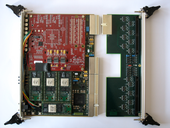
Figure 1.26: The Level 2 trigger board equipped with an Avent evolution board and 4 Mini-Modules (on the left) and a rear I/O board for the conversion of 64 LVDS links from the Front End electronics (on the right).

The Level 2 trigger system is receiving the data from the Front End (FE) electronics on 64 LVDS links. The received data contain two binary images of the camera. Each image is made up of 2048 pixels on an equilateral triangular grid (see figure 1.27).

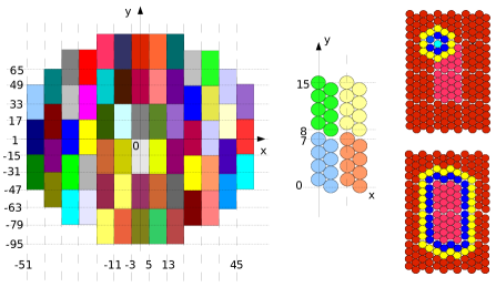
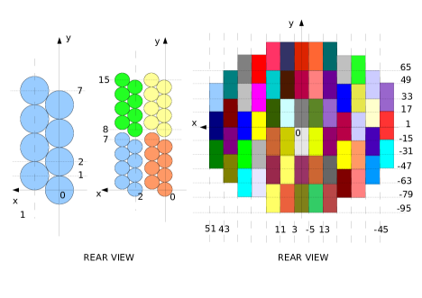
Figure 1.27: right : The camera of the LCT is composed of 64 drawers. Each drawer contains 2 Front End (FE) boards and each FE board carries 8 pixels. The 2048 pixels of the camera are on an equilateral triangular grid. middle : Local integer coordinate frame used for Hillas parameter estimation. left : First and second neighbors to the pixels on 4 FE boards in a pair of drawers.

The EB is equipped with the Micron 32 MB DDR SDRAM memory. It can be used by the PPC to hold code and data. The Virtex-4 FPGA is accessible through 76 user I/Os and is connected to 32M x 16 of DDR memory. Both boards hold a 100 MHz oscillator for clocking purposes.

The EB is in charge of receiving the data from the FE boards, through the backplane. Additional information about the stereoscopic nature of the incoming event reaches the EB through the front panel. The Level 2 system sends the algorithm decision (L2A or L2R) as an output to the Data Acquisition System (DAQ). The data acquisition FIFOs buffer have a capacity of 50 events, and is used to hold the camera data while awaiting for the Level 2 trigger response. The capacity of the buffer sets an upper bound on the latency of the Level 2 system, constraining the real-time implementation of the Level 2 trigger algorithms.

1.9.2 The algorithm implementation

If the processed event is tagged as stereo, the Level 2 trigger uses its selection algorithm to decide if the event will be issued as accepted (L2A) or rejected (L2R). The algorithm proceeds as follow:

1. Set to 0 all pixels in $map_{1}$ that are not in clusters of 3 at least $\rightarrow\widetilde{map}_{1}$
2. IF $\widetilde{map}_{1}=0$ THEN Reject ELSE
	3. Set to 0 all isolated pixels in $map_{1}$ $\rightarrow\widehat{map}_{1}$
	4. Compute Hillas parameterd of $\delta_{1}\widehat{map}_{1}+(\delta_{2}-\delta_{1})map_{2}$
	5. Compute distance $\Delta$ from center of gravity (COG) to target $(x_{c},y_{c})$
	6. IF $\Delta\geq\tau_{\textrm{{\tt COG}}}$ THEN Reject ELSE Accept

where ${map}_{1}$ and ${map}_{2}$ are the two input binary maps associated with threshold values of $\delta_{1}$ and $\delta_{2}$, $(x_{c},y_{c})$ are the pointed target’s coordinates in the camera plane and $\tau_{\textrm{{\tt COG}}}$ is the decision threshold on the nominal distance $\Delta$ between the COG of the event and the target position.

The Level 2 trigger is build as a pipeline system. The first step of the Level 2 pipeline is a transposition of the input 64$\times$64 binary data matrix. The step is performed before the matrix is available to the PPC in a dedicated cacheable memory block. The first half of the data represents the binary camera image with the true values for pixels above threshold $\delta_{1}$ ($map_{1}$). The second half is a $map_{2}$ obtained for the pixel threshold $\delta_{2}$, respectively.

The 32 bit words are then read by the PPC from the block.

Each byte corresponds to the 8 pixels from one FE board. The geographical position of pixels follows a constant logical pattern. The auxiliary processor of the V4FX12 is used to achieve a parallel implementation of the non-linear filters in step 1 and 3. This has been built using logic AND and OR gates. In this way denoising (Step 1) was implemented by convolving $map_{1}$ with the filter:

$$\widehat{map}_{1}(i)=map_{1}(i)\wedge\left(\bigcup_{j=1..6}map_{1}(i_{j})\right)\,,$$ (1.18)

where $i_{j}$ is used to index the 6 nearest neighbors of a pixel. The similar filter is used to detect the cluster of at least 3 or 4 pixels.

A fast implementation of step 4 is obtained by reorganizing the wighted sums that define the $1^{st}$ and $2^{nd}$ order moments of the input data. Computing the $1^{st}$ and $2^{nd}$ order moments of the denoised combined map is common for the estimation of Hillas parameters and other parameters of interest (Hillas, 1985). It can be defined as:

$$m_{x}=\sum_{i}m_{i}x_{i}\,,\quad \quad m_{y}=\sum_{i}m_{i}y_{i}\,,$$ (1.19)

$$m_{xx}=\sum_{i}m_{i}x_{i}^{2}\,,\quad \quad m_{yy}=\sum_{i}m_{i}y_{i}^{2}\,,$$ (1.20)

$$m_{xy}=\sum_{i}m_{i}x_{i}y_{i}\,,\quad \quad m=\sum_{i}m_{i}\,,$$ (1.21)

where $i$ indexes the 2048 pixels in the processed data maps, and $m_{i}$ is the weight assigned to pixel $i$. The binary maps $\widehat{map}_{1}$ and ${map}_{2}$ can be processed separately and the sums are profitably rearranged for an efficient hierarchical computation of the moments.

First, a byte-addressable look-up table (LUT) is used to compute the $1^{st}$ and $2^{nd}$ order moments on each FE board. These are combined locally to compute these statistics on each of the 64 pairs of drawers. This local summation requires the LUT outputs to be properly translated depending on the position of a given FE board in the current pair of drawers. Summation over the 64 pairs of drawers requires an additional transformation of these statistics to account for the translation and scaling of the local frame. This requires a move of the current drawer to its correct position within the global coordinate frame of the camera. In the end, the contributions of the two binary maps are linearly combined with weights $\delta_{1}$ and $\delta_{2}-\delta_{1}$ providing final 32 bit integer statistics $m_{yy}$, $m_{xy}$, $m_{xx}$, $m_{y}$, $m_{x}$ and $m$ for the combined map.

With this fast implementation, the PPC computes the first and second order moments of the input data in a maximum of 18000 clock cycles. For an even faster execution time, given that these statistics will most often be estimated for low energy events when only very few pixels are high in $\widehat{map}_{1}$ and even less in ${map}_{2}$, it is worth checking if a byte is zero before using the LUT. As a result the computation time will vary almost linearly with the number of active bytes in the data.

The algorithm proposed in section 1.7 uses only the first-order statistics to compute the nominal distance in finite precision:

$$\Delta=\sqrt{(\frac{m_{y}}{m}-y_{c})^{2}+3(\frac{m_{x}}{m}-x_{c})^{2}}\,,$$ (1.22)

where the factor $3$ is due to the equilateral triangular grid and the accompanying $\sqrt{3}$ left out in the moment computation for simplicity. The specified precision on the target coordinates is $1/32^{\textrm{th}}$ of the unit length, giving the precision to which the COG coordinates have to be computed.

1.9.3 Experimental timing results

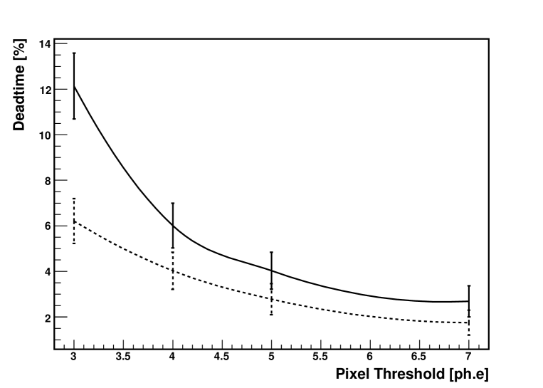
Figure 1.28: Estimated deadtime of the PPC in the single FPGA implementation of the Level 2 trigger system. The continuous and dashed lines correspond to Level 1 pixel mulitiplicities equal to 3 and 4 respectively.

The design and real time implementation of the Level 2 algorithm is constrained by the maximum latency. If the Level 1 rate is of the order of 100 kHz, the maximum latency of the Level 2 trigger is $\sim$500 $\mu$s. The minimum time between two events is then 10 $\mu$s. If the Level 1 rate is reduced to 5 kHz, the maximum latency of the Level 2 trigger increases to 10 ms and the minimum mean time between two events is 200 $\mu$s.

The Level 2 architecture was tested with timing experiments in order to benchmark the performance of the proposed hardware, firmware and software solution for the Level 2 trigger system. With this setup, a stable behavior of the system was observed up to a maximum Level 1 rate slightly above 10 kHz. The multi-FPGA system could sustain a maximum mean rate close to 30 kHz. A more realistic estimation of the maximum acceptable Level 1 rate is plotted on figure 1.28. This results were obtained for the first implementation of the Level 2 trigger system. The dead-time estimate is based on the simulated rates reported in sections 1.8 and on time measurements of the different elementary steps in the Level 2 trigger pipeline. For typical Level 1 trigger conditions (multiplicity 3 or 4 and pixel threshold between 3 and 7) the estimated average processing time is $\sim$ 37 $\mu$s, which corresponds to a maximum Level 1 trigger rate of 27 kHz. Actually, for these trigger conditions, the system occupancy is estimated to be $\leq 20$ % as shown on figure 1.28. The proposed multi-FPGA system will provide thus a safe margin. However, the real Level 1 and Level 2 trigger rate have to be determined on site.

1.10 Conclusions

The Level 2 trigger is going to be used to reduce the trigger rate of the LCT at low energy. The principle of the Level 2 trigger is to build a 2-bit (“combined”) map of the camera pixels at the time of trigger. The NSB events can then be rejected by demanding clusters of pixels on the combined map. Further rejection of the hadronic background can be obtained by using quantities such as the COG of the pixels above a pixel threshold. A possible, illustrative, algorithm for the Level 2 trigger system has been described in section 1.7. This algorithm shows that the required rejection of the NSB and isolated muon triggers is achievable.

The hardware and software integration into the LCT camera of the previously described system based on a single V4FX12 has been achieved. The Level 2 system is already fully integrated in the H.E.S.S. II acquisition system and is currently undergoing tests with real data.

Part II Data analysis and modeling of PKS 1510-089

2.1 Introduction

The observations of the FERMI satellite in the high energy (HE) range resulted in the identification of 1873 sources, according to the second FERMI catalog (Nolan et al., 2012). Among these 1873 sources majority are blazars. Blazars are very luminous active galactic nuclei (AGNs) with a relativistic jet pointing toward the observer.

The broadband spectrum of blazars is dominated by non-thermal emission produced in the jet (Blandford & Rees, 1978). The spectral energy distribution (SED) is characterized by two broad spectral components. One component, which extends from the radio to optical/UV/X-rays, peaks at low energy, and is produced by the synchrotron radiation of relativistic electrons. The second one, from X-rays to $\gamma$-rays, peaks in the HE range and in most current interpretations is produced by inverse Compton (IC) radiation with as possible source of seed photons either the synchrotron radiation, or the broad line region (BLR) or the dusty torus (DT).

Blazars can be divided into two classes: Flat Spectrum Radio Quasars (FSRQs) and BL Lac objects. FSRQs are distinguished from BL Lac objects by the presence of broad emission lines, which are not found in BL Lac objects. The FSRQs have HE components much more luminous than low energy ones. The seed photons for IC radiation most probably come from BLR. The seed photons, for BL Lacs objects, probably come from the synchrotron radiation, and both spectral components have comparable luminosities.

According to the prediction of Moderski et al. (2005), the spectra of blazars should have a cut-off at a few GeV due to the Klein-Nishina effect, if the high energy component is produced by IC of photons reemitted in BLR. Spectral breaks at a few GeV have been found in the $\gamma$-ray spectra of many FSRQs and BL Lacs (Abdo et al., 2011). The most prominent example is 3C 454.3 (Abdo et al., 2009). In addition, the luminous IR-UV photon field, from the BLR and the DT, can cause a strong absorption of HE and VHE photons by electron-positron pair production (Donea & Protheroe, 2003; Liu & Bai, 2006).

The other possible explanation of the spectral break involves photo-absorption by He II and Ly$\alpha$ (Poutanen & Stern, 2010). Gamma rays photo-absorbed by He II recombination (54.5 eV) and Ly $\alpha$ (40.8 eV) photons from the BLR would create a break at $\sim$5 GeV.

The number of known blazars in HE range is larger than 1000, but in VHE range only about 50 blazars have been detected so far (Errando & for the VERITAS Collaboration, 2012). Up to now, only BL Lacs objects, from the blazar class, were clearly detected as VHE sources.

Recently however, Cherenkov telescopes have detected 3 FSRQ in sub-TeV range. The first detected object was 3C 279, observed with the MAGIC telescope (Aleksić et al., 2011b). Two additional FSRQs are 4C 21.35 detected by the MAGIC telescope (Aleksić et al., 2011a) and PKS 1510-089 detected with H.E.S.S. (Hauser et al., 2011). The detection of these objects shows that FSRQs can also emit photons in the VHE range. The emission in this energy range is very difficult to explain by inverse Compton of photons from BLR.

2.2 Unification schemes of active galaxies

The unified theory of AGNs has been developed since the 70s (Antonucci, 1993). The basic idea of the unification assumes that all of the active galaxies have similar internal structure of their nuclei, but their appearances depend on their orientations. Figure 2.1 shows the model proposed by Urry & Padovani (1995).

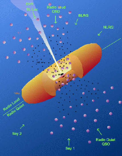
Figure 2.1: A schematic diagram of AGN.

This model assumes that all the AGNs are powered by accretion of surrounding matter onto the supermassive black hole located in the center of the host galaxy. The accreting matter forms a geometrically thin accretion disk and corona heated by magnetic or viscous processes. Farther out there is a geometrically thick DT. The emission from the accretion disk is reprocessed in DT and BLR. The fraction of reprocessed emission by BLR and DT ($\xi_{BLR,DT}$) can not be larger than 1. The typical values of $\xi_{BLR,DT}$ are in the range of $\sim$ 0.1–0.3 Nalewajko et al. (2012).

The AGNs are divided to many subclasses. The most common classifications based on the properties like an appearance (if the source is observed as a point-like or a clear galaxy host), an presence or an absence of the broad or narrow line regions, a variability or a polarization. The most popular groups are

• radio-load active galaxies (10%)

• radio-quiet active galaxies (90%)

• Seyfert galaxies named after Carl Seyfert, who pointed out the first six Seyfert galaxies. This group was later subdivided into two types (according to presence or absence of the broad or narrow emissions lines)

• Optically Violently Variable (OVV), this class is marked by exceptionally rapid and large amplitude variability in the optical band

The further classification distinguishes also quasars group, which consists of objects found at large distances with very bright emission from the jet. Quasars include radiogalaxies and blazars.

2.3 Blazar sequence

Blazars are the most luminous AGNs. Their emission is dominated by the boosted radiation from the jet, and their spectra consist of two broad components. The low-frequency component (LFC) has a peak in the IR-X-ray range, while the high-frequency component (HFC) has a peak in MeV to TeV range. Both components are highly variable, with time scale ranging from years to the fraction of a day. Blazars are also characterized by high radio and optical polarization, and in many cases strong $\gamma$-ray emission.

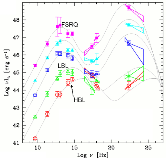
Figure 2.2: Blazar Sequence. Figure credited from Donato et al. (2002) and Fossati et al. (1998).

The superimposed blazar spectral energy distributions (SEDs) from figure 2.2 suggest the correlation between the luminosities and the peaks positions. The sequence is characterized by an increasing synchrotron peak frequency, a decreasing overall luminosity and a decreasing dominance of the $\gamma$-ray emission over the synchrotron component. Fossati et al. (1998) based on this behavior elaborated an unified view of the SEDs called the blazar sequence (see figure 2.2).

FSRQs and BL Lacs occupy the opposite sides of the blazar sequence. In the case of FSRQs, the peaks of low-frequency ($\nu_{syn}$) components are shifted toward lower frequencies as compared to the BL Lacs. The broad-band spectrum of FSRQs is characterized by a large luminosity ratio of their high-frequency and low-frequency spectral components. This luminosity ratio can reach values up to 100. In the case of BL Lac objects, the luminosities of high and low frequency components are comparable.

Since the location of the low-frequency peak is quite broad, blazars are sometimes further divided into sub-groups based on the peak position ($\nu_{syn}$). Blazars with $\nu_{syn}\leq 10^{14}$ Hz are called low-synchrotron-peaked (LSP). LSP group contains both FSRQs and LSP BL Lac objects (LBLs). Blazars with a low-frequency peak located in frequency range $10^{14}$ Hz $\leq\nu_{syn}\leq 10^{15}$ Hz are called intermediate-synchrotron-peaked (ISP). The ISP group primarily consists of intermediate BL Lac objects (IBLs). Finally, the last group, high-frequency peaked (HSP) BL Lac objects, is characterized by $\nu_{syn}>10^{15}$ Hz (Abdo et al., 2010c). The sequence then appears as follows: FSRQ$\rightarrow$LBL$\rightarrow$IBL$\rightarrow$HBL. The FERMI satellite provided a large sample of sources with spectra measured over almost 4 years, the blazar classification seems to be much more complicated (Giommi et al., 2012; Meyer et al., 2011). However, here I use this simplified approach to illustrate the basic properties of the blazar class.

2.4 Accretion disk

Lets assume a ”standard” (Shakura & Sunyaev, 1973) accretion disk. The accretion disk is optically thick and emits a large amount of thermal radiation from infrared to ultraviolet. The thermal emission of accretion disks peak in the UV (”big blue bump”). In blazars the UV observations during the low state of synchrotron radiation can be used to estimate the upper limit of the accretion disk luminosity $L_{d}$. Following the prescription given by King (2008) and Ghisellini et al. (2009), the temperature of the disk is given by:

$$T^{4}_{disk}(r)=\frac{3R_{S}L_{d}}{16\pi\epsilon\sigma_{SB}r^{3}}\left[1-\left(\frac{3R_{S}}{r}\right)^{\frac{1}{2}}\right]\,,$$ (2.1)

where $\sigma_{SB}$ is the Stefan Boltzman constant, $R_{S}$ is the Schwarzschild radius of a black hole, $3R_{S}$ refers to the last stable circular orbit for the Schwarzschild black hole and the disk extends up to 500 $R_{S}$, $\epsilon\,\sim\,0.05\,-\,0.42$ is the efficiency of rest-mass conversion, which depends on the inner boundary conditions, and the black hole spin. The accretion efficiency, $\epsilon$, is linked to the bolometric disk luminosity, $L_{d}$, and to the accretion rate $\dot{M}$ as $L_{d}=\epsilon\dot{M}c^{2}$. The radiation region of the disk extends from $\simeq 3R_{S}$ to 500 $R_{S}$. The disk temperature peaks at $R\simeq 4R_{S}$.

2.5 Broad line region

The clouds surrounding the central part of AGN are ionized by ultraviolet radiation from the accretion disk. The clouds reprocessed the disk radiation and produce emission lines, which are broadened due to high velocity of the cloud around the central black hole. This part of the AGN model is called the broad lines region (BLR). The luminosity of the BLR is proportional to the $L_{d}$ as

$$L_{BLR}=\xi_{BLR}L_{d}\,,$$ (2.2)

where $\xi_{BLR}\simeq 0.1-0.3$ is the fraction of the disk radiation reprocessed in BLR. The radius of the BLR can be derived using the method called ”emission-line reverberation mapping” (Peterson et al., 2004). This technique uses the time-lag of the emission line light curve with respect to the continuum light curve to determine the light crossing size of the BLR in AGNs. The reverberation studies resulted in the empirical relationship between $R_{BLR}$ and the optical continuum luminosity at 1350Å (Pian et al., 2005):

$$R_{BLR}=(22.4\pm 0.8)\left[\frac{\lambda L_{\lambda}(1350\mbox{\AA})}{10^{44}\mbox{erg\, s}^{-1}}\right]^{0.61\pm 0.02}\,\mbox{light days}\,.$$ (2.3)

The energy density of BLR radiation fields $u_{BLR}$ is constant within $R_{BLR}$ and declines as $r^{-2}$ outside:

$$u_{BLR}\simeq\frac{\xi_{BLR}L_{d}}{4\pi cR_{BLR}^{2}}\frac{1}{1+(r/R_{BLR})^{2}}.$$ (2.4)

2.6 Dusty torus

The radiation from accretion disk is also reprocessed by the dust, which forms a torus located outside the accretion disk. The luminosity of the DT can be expressed as:

$$L_{DT}=\xi_{DT}L_{d}\,,$$ (2.5)

where $\xi_{DT}$ is the fraction of reprocessed emission. The reflectivity, in this case, is of the order of $\sim$ 0.1 (Ghisellini et al. 2009).

The temperature of the DT (Błażejowski et al., 2000) is expressed as

$$T_{DT}^{4}=\left(\frac{L_{d}}{4\pi\sigma_{SB}R_{DT}^{2}}\right)\,.$$ (2.6)

The temperature of the dust gives the characteristic frequency of the DT radiation field:

$$h\nu_{DT}\simeq 3.92\,k\,T_{DT}\,.$$ (2.7)

The size of DT is approximated by $R_{DT}\simeq 2.9\,$pc$\times T^{-2.6}_{3}$ (Tavecchio & Ghisellini, 2008; Nenkova et al., 2008; Sikora et al., 2009), where the dust temperature $T_{3}=T\times 1000$.

Within the $R_{DT}$, the energy density, $u_{DT}$ of external radiation fields, is roughly independent of the radius, and outside decreases with distance:

$$u_{DT}\simeq\frac{\xi_{DT}L_{d}}{4\pi cR_{DT}^{2}}\frac{1}{1+(r/R_{DT})^{2}}\,.$$ (2.8)

2.7 Jets

Jets are streams of hot plasma, which moves with relativistic speeds. Jets transport the energy up to distances of many kpc. Around 10% of the jet energy is dissipated in the very first parsecs. When the jet collide with the intergalactic matter it produces luminous lobes.

The exact mechanism of the jet formation and collision is unknown. It has been suggested that it has to be mediated by the magnetic field in the inner part of AGN (Blandford & Znajek, 1977). Its strong collimation suggest a large density of magnetic energy.

Jets at small distances (subparsec) are dominated by magnetic field (Blandford, 1983). At larger scales the energy of the jets is dominated by matter (Sikora et al., 2005). The majority of emission is produces at the parsec scale.

The radio observations of superluminal motion impliy that matter in the jet reaches relativistic speeds. Other observations suggest that jets may have a Lorentz factors $\Gamma$ of the order of 10 to 20. The observed luminosity of objects moving with a large Lorentz factor is boosted by the Doppler effect, where the Doppler factor is defined as

$${\cal D}=\frac{1}{\Gamma\left(1-\beta_{\Gamma}\cos\theta_{obs}\right)}\,,$$ (2.9)

where $\theta$ is the angle between the direction of the source motion and the line of sight between the source and the observer, and $\beta_{\Gamma}=\sqrt{\Gamma^{2}-1}/\Gamma$. The observed radiation flux is

$$\nu_{obs}F_{\nu_{obs}}={\cal D}^{4}\frac{\nu L_{\nu}}{4\pi d_{L}^{2}}\,,$$ (2.10)

where $\nu=\nu_{obs}(1+z)/{\cal D}$, $L_{\nu}$ is the source luminosity and $d_{L}$ is the luminosity distance.

2.8 Models of jet emission

The spectrum energy distribution (SED) is composed of two broadband components. There is an agreement that the lower component, which peaks at infrared to X-rays, is produced by the synchrotron emission of relativistic electrons within the jet. The non-thermal character of emission is confirmed by the observations of rapid variability on time scales of days or less throughout the entire wavelength range (Wagner & Witzel, 1995) and high polarization (even 40%) in the radio and the optical range (Mead et al., 1990).

The origin of the high energy component is far more debated. The most common interpretation suggests that the origin is the inverse Compton (IC) emission of relativistic electrons, or pairs – the so-called leptonic models. The obvious choice of seed photons would be the synchrotron radiation from the same population of electrons. The family of such scenarios is called the synchrotron self-Compton (SSC) models, and seems to explain well the spectra of BL Lac objects, where the lack of any emission and absorption lines suggests the absence of any external radiation fields. For more details see Konigl (1981); Marscher & Gear (1985); Ghisellini & Maraschi (1989).

For FSRQs, SSC models cannot easily explain the large difference of luminosities between the low-frequency component and high-frequency component peaks observed (Sikora et al., 2009). The luminosity of the high energy component exceeds the luminosity of the low energy component by a factor 10 to 100 times. An external source of seed photons for IC was proposed to explain such a large difference of the peak luminosities (Dermer et al., 1992; Dermer & Schlickeiser, 1993; Blandford & Levinson, 1995; Sikora et al., 1994).

In addition to the electrons, protons are an inevitable component of the jet. It is worth noting that even if the number of electrons largely exceed the number of protons, because of the large mass difference $m_{p}/m_{e}\sim 1836$, the jet power may still be dominated by ultra-relativistic protons. In some scenarios, the so-called hadronic models, protons are also involved in the radiation mechanisms of jet emission. Such hadronic models were discussed for example by Mücke et al. (2003); Boettcher (2010); Cerruti et al. (2012).

The direct proton synchrotron emission or proton IC process are much less efficient in emitting radiation than the same processes involving electrons ($\sigma_{T}\sim m_{e/p}^{-2}$). The proton cooling time scale is too long to explain the emission of blazars. To overcome this difficulty some hadronic models involve pion production. The high energy protons interacting with low energy photons may produce pions:

$$\begin{array}[]{ccc}&p+\gamma\rightarrow n+\pi^{+}\,,&\\ &p+\gamma\rightarrow p+\pi^{0}\,.&\\ \end{array}$$ (2.11)

The pions initiate cascades of high energy particles. The neutral pions can decay to TeV photons. The hadronic models require an extreme environments to explain blazars emission. They require in particular a magnetic field of the order of 100 G, or an extreme number of protons with large Lorentz factors (see e.g. Sikora et al. (2009) for a current review).

In the present thesis the leptonic model is used to explain the emission of blazar PKS 1510-089.

2.9 Internal shock scenario

The observations of blazars show a correlated variability of the low and high peak components with a time scale as low as hours suggesting a compact region of emission (Aharonian et al., 2005). This may suggest that a significant fraction of the jet energy is dissipated at a sub-parsec scale from the center of the region of emission. The energy dissipation can be explained by an internal shock scenario (Sikora et al., 1994; Spada et al., 2001), or the reconnection of magnetic field (Romanova & Lovelace, 1992; Blackman, 1996). Both approaches are sufficient to produce an efficient acceleration of particles.

The internal shock scenario assumes some instability in the central part of the active galactic nuclei, which results in the ejection of blobs of matter. The jet consists of blobs of different velocity, masses, and densities (Rees, 1978). The blobs with the larger velocity catch up with those with smaller velocities, and a nonelastic collision occur. Consider two blobs of matter with velocities $\Gamma_{1}<\Gamma_{2}$ and masses $m_{1}$ and $m_{2}$. Conservation of energy and momentum implies that the dissipation ”efficiency” $\eta$ of the total bulk kinetic energy during the collision is (Moderski et al., 2004):

$$\eta=1-\Gamma_{sh}\frac{m_{1}+m_{2}}{\Gamma_{1}m_{1}+\Gamma_{2}m_{2}}\,,$$ (2.12)

where $\Gamma_{sh}=(1-\beta_{sh}^{2})^{-1/2}$ is the bulk Lorentz factor of the forward shell after the blobs collision, and $\beta_{sh}$ the shell velocity is:

$$\beta_{sh}=\frac{\beta_{1}\Gamma_{1}m_{1}+\beta_{2}\Gamma_{2}m_{2}}{\Gamma_{1}m_{1}+\Gamma_{2}m_{2}}\,.$$ (2.13)

Typically $\eta$ is of the order of 5% - 10% (Spada et al., 2001). The efficiency of dissipation increases when the velocity difference is large. The largest efficiency is obtained during the first collisions, close to the jet base (Spada et al., 2001). Assuming that the blobs velocities before the collisions are $v_{1}$ and $v_{2}$, respectively, ejected with initial separation $\Delta r_{ej}$, the blobs will collide at a distance:

$$R_{0}=\frac{v_{2}}{v_{2}-v_{1}}\Delta r_{ej}\simeq\frac{2\Gamma^{2}_{1}\Gamma^{2}_{2}}{\Gamma^{2}_{2}-\Gamma^{2}_{1}}\,.$$ (2.14)

This region is called the blazar zone, where the majority of the non-thermal emission is produced. Collisions of blobs produce a shock structure, which accelerates particles to relativistic energies. In the absence of a detail model of particle acceleration the resulting distribution of particles is assumed to be a pawer law or a broken power law.

In this thesis the electron injection function is assumed to take the broken power law form

$$Q_{\gamma}=K_{e}\frac{1}{\gamma^{p}+\gamma_{\rm br}^{p-q}~{}\gamma^{q}}\,,$$ (2.15)

where $K_{e}$ is the normalization factor, $p$ and $q$ are spectral indices of the injection function at the low and high energy limits, respectively, and $\gamma_{\rm br}$ is the break energy.

2.10 Synchrotron radiation

When a relativistic electron with a Lorentz factor $\gamma$ is moving in a magnetic field $B$, it emits non-thermal radiation with $\nu_{syn}=4/3\gamma^{2}\nu_{L}$, where $\nu_{L}=eB/(2\pi m_{e}c)=2.8\times 10^{6}\frac{B}{1G}\,$Hz. The average photon energy is thus:

$$\langle\varepsilon\rangle\simeq\frac{4}{3}\gamma^{2}\frac{B}{B_{cr}}~{},$$ (2.16)

where

$$B_{cr}\equiv\frac{m_{e}^{2}c^{3}}{e\hbar}\simeq 4.414\times 10^{13}{\rm G}~{}.$$ (2.17)

and the energy is expressed as $\varepsilon=h\nu/m_{e}c^{2}$.

The rate of synchrotron cooling is calculated according to the formula:

$$\dot{\gamma}=\frac{4c\sigma_{T}}{3m_{e}c^{2}}\gamma^{2}u_{B}\,,$$ (2.18)

where $u_{B}=B^{2}/8\pi$ is the magnetic field energy density.

2.11 Inverse Compton radiation

Consider a collision between a soft (low energy) photon and a relativistic electron of velocity $\beta c$. If energy of the photon is $h\nu$, the incidence angle $\theta$, and the electron velocity $\beta$ then the photon is boosted in energy to:

$$\frac{\nu}{\nu_{0}}=\frac{1+\beta\cos{\theta_{0}}}{1-\beta\cos{\theta}+\frac{h\nu_{0}}{\gamma m_{e}c^{2}}(1+\cos(\theta-\theta_{0}))}\,.$$ (2.19)

When the ratio between the energy of the photon and the energy of the electron before the collision $\gamma\frac{h\nu_{0}}{(m_{e}c^{2})}$ is $\ll$ 1, the interaction proceeds in the, so-called, Thomson regime. The electron energy loss in a single collision is negligible and the photon collision is elastic in the center-of-momentum frame.

The maximum energy gain of a photon occurs in $\theta=\theta_{0}=0$ and $\beta\rightarrow 1$. Then $\frac{\nu}{\nu_{0}}\simeq 4\gamma^{2}$. The average energy gain at given $\theta_{0}$ over all possible interaction angles is

$$\left\langle\frac{\nu}{\nu_{0}}\right\rangle=\gamma^{2}(1+\cos{\theta_{0}}).$$ (2.20)

The rate of IC energy losses of relativistic electron, isotropically distributed photons is

$$|\dot{\gamma}_{T}|=\frac{4c\sigma_{T}}{3m_{e}c^{2}}\gamma^{2}u_{0},$$ (2.21)

where $u_{0}$ is the total energy density of the radiation field ($u_{0}=\int_{\epsilon_{min}}^{\epsilon_{max}}u_{\epsilon}d\epsilon$), $u_{\epsilon}$ is the energy density distribution of the ambient photons.

2.12 The Klein-Nishina effect

When the photon energy becomes comparable to the electron energy or larger ($\gamma\frac{h\nu_{0}}{m_{e}c^{2}}>1$), the electron may loose most of its energy during a single collision. In that case the IC cross-section has to be expressed by the full Klein-Nishina (KN) formula (Moderski et al., 2005). The cross-section is reduced as compared to the Thomson regime when the photon energy becomes larger. The main effect is a reduction of the electron energy loss rate:

$$\dot{\gamma}=\dot{\gamma}_{T}\,F_{KN}\,,$$ (2.22)

where $\dot{\gamma}_{T}$ is given by equation (2.21) and a factor $F_{KN}$ is given by

$$F_{KN}={1\over u_{0}}\int_{\epsilon_{min}}^{\epsilon_{max}}f_{KN}(b)u_{\epsilon}d\epsilon\,,$$ (2.23)

where $b=4\gamma\epsilon$. The $b=1$ corresponds to the transition between the Thomson and KN scattering regimes. The function $f_{KN}(b)$ is given by Moderski et al. (2005):

$$f_{KN}(b)=\frac{9g(b)}{b^{3}}~{},$$ (2.24)

$$g(b)=\left(\frac{1}{2}b+6+\frac{6}{b}\right)\ln(1+b)-\left(\frac{11}{12}b^{3}+6b^{2}+9b+4\right)\frac{1}{(1+b)^{2}}-2+2{\rm Li}_{2}(-b)$$ (2.25)

where $Li$ is dilogarithm and $b=4\varepsilon_{0}\gamma$.

For $b\ll 1$ (Thomson limit), $f_{KN}\simeq 1$; for $b\gg 1$ (KN limit), $f_{KN}\simeq[9/(2b^{2})](\ln b-11/6)$. For $b\leq 10^{4},$ $f_{KN}(b)$ can be approximated by $f_{KN}\simeq{1\over(1+b)^{1.5}}$.

Electrons, for which cooling by Comptonisation is inefficient, are loosing more energy throughout the synchrotron emission. Usually, the effect of Klein-Nishina is seen as an excess of synchrotron luminosity and the hardening of synchrotron spectrum, while the Compton component shows a cut-off.

2.13 Absorption

The influence of low energy photons present in the Universe on the propagation of the HE gamma-rays was pointed out by Gould & Schréder (1967). The fundamental process responsible of the HE $\gamma$-ray absorption is the electron-positron pair production:

$$\gamma_{HE}+\gamma_{LE}\rightarrow e^{+}+e^{-}\,.$$ (2.26)

The observed HE $\gamma$-ray spectrum after attenuation is

$$F_{obs}=F_{int}e^{-\tau}\,,$$ (2.27)

where $e^{-\tau}$ is the attenuation, $\tau$ is the optical depth, and $F_{int}$ is the intrinsic spectrum of the source. The optical depth given by Gould & Schréder (1967) is

$$\tau(E)=\int dl\int_{\cos\theta_{min}}^{\cos\theta_{max}}d\cos{\theta}\frac{1-\cos{\theta}}{2}\int_{E_{th}}^{\infty}d\epsilon n(\epsilon)\sigma(E,\epsilon,\cos{\theta})\,,$$ (2.28)

where $dl$ is the differential path travelled by the HE photon, $\theta$ is the angle between the momenta of HE and LE photons. The energy of HE photon is (1 + z)E and the energy of LE photon is (1 + z)$\epsilon$, where E and $\epsilon$ are the observed photon energies at z = 0. The low energy photons density number is $n(\epsilon)d\epsilon\,\mbox{cm}^{-3}$. The cross-section of pair production is given by Bi & Yuan (2008):

$$\sigma(E,\epsilon,\cos{\theta})=\sigma_{T}\frac{3m_{e}^{2}}{2s}\left\{-\frac{p_{e}}{E_{e}}1+\frac{4m_{e}^{2}}{s}+\left[1+\frac{4m_{e}^{2}}{s}\left(1-\frac{2m^{2}_{e}}{s}\right)\right]\log\frac{(E_{e}+p_{e})^{2}}{m^{2}_{e}}\right\}\,,$$ (2.29)

where $s=2E\epsilon(1-\cos\theta)(1+z)^{2}$, $E_{e}=\sqrt{s}/2$, and $p_{e}=\sqrt{E_{e}^{2}-m_{e}^{2}}$.

The condition for pair production is $E\epsilon(1+z)^{2}(1-\cos\theta)>2(m_{e}c^{2})^{2}$, which corresponds to a threshold energy of

$$E_{th}=\frac{2(m_{e}c^{2})^{2}}{\epsilon(1+z)^{2}(1-\cos{\theta})}\,.$$ (2.30)

HE photons can be absorbed by several backgrounds of LE photons during their travel to the observer. The first source of LE photons is an extragalactic background light (EBL). The EBL is the IR/UV radiation generated by stars (UV) or radiation emitted through the absorption and re-emission of star light by dust in galaxies (IR). The EBL models have been reviewed by, e.g. Hauser & Dwek (2001) and recently new constraints have been provided by Meyer et al. (2012) using the FERMI data and Abramowski et al. (2012) using the H.E.S.S. observations of the brightest blazars.

For characteristic frequency of EBL photons of $\epsilon_{EBL}\simeq$0.1 eV the photons with energy above 5 TeV will be affected by absorption:

$$\frac{E_{th}}{0.1\,\mbox{eV}}\sim 5.2\frac{E}{1\,\mbox{TeV}}\,.$$ (2.31)

The distribution of angles $\theta$, at which background photons can collide with the HE photons is flat when the photon is traveling over cosmological distances, therefore, the $\cos\theta$ of the scattering angle (see equation 2.28) changes from -1 to 1. The differential path $dl$ travelled by the HE photon can be calculated using equations (3.33) or (3.34).

The second possibility of absorption arises from the photon fields present in the blazar itself. When the HE photon is produced in the jet, it has to travels through two fields of LE photons: the broad line region (BLR) and IR radiation from the dusty torus (DT), depending on where it was emitted.

The characteristic frequency of the BLR radiation is of the order of 10 eV. Since, the energy of BLR photons is larger than that of DT photons, the threshold energy of pair production is smaller and HE photons can be absorbed above energies of a few GeV. To avoid significant absorption by BLR photons, the blazar zone where HE photons are emitted, has to be located outside of BLR, otherwise the HE emission is significantly absorbed. The photon number density of external radiation (from BLR and DT) decreases with distance as in equation (2.4) and (2.8), respectively. When HE photons propagates inside the BLR or DT then the $\theta$ distribution is flat, therefore the $\cos\theta$ in the equation (2.28) ranges from -1 to 1. However, outside the BLR or DT, the $\theta$ can have values ranging from $\theta_{min}=(\pi+{\rm atan}(R_{BLR,DT}/r))$ to $\theta_{max}=(\pi-{\rm atan}(R_{BLR,DT}/r))$.

The distance $dl$ is measured from the place where the gamma photons are emitted up to the distance where the energy densities of BLR or DT are negligible.

2.14 The PKS 1510-089 blazar

PKS 1510-089 ($\alpha_{\rm J2000}=15^{\rm h}12^{\rm m}50.5^{\rm s}$, $\delta_{\rm J2000}=-09^{\rm d}06^{\rm m}00^{\rm s}$) at redshift $z=0.361$ is the FSRQ detected in the MeV-GeV band by EGRET (Hartman et al., 1999). It is characterized by a highly relativistic jet that makes a $3^{\circ}$ angle relative to the line of sight (Wardle et al., 2005). The radio jet of PKS 1510-089 is curved and shows an apparent superluminal motion as high as 45 times the speed of light (Homan et al., 2001, 2002). The first large multi-wavelength campaign on PKS 1510-089 took place in August 2006 (Kataoka et al., 2008) and involved Suzaku, Swift and ground-based optical and radio instruments. The campaign resulted in a broadband spectrum ranging from $10^{9}$ to $10^{19}\,$Hz, which was succesfully modeled within the internal shock scenario. Kataoka et al. (2008) focused their work on the explanation of the soft X-ray part of the SED, where an excess of emission has been observed, which if interpreted as bulk-Compton radiation, allowed to obtain the e⁺e^- to proton ratio. In the case of PKS 1510-089, the ratio was estimated to be of the order of $10$. This implies that although the number of e⁺e^- pairs is larger then the number of protons, the power of the jet is dominated by the latter.

As an alternative interpretation, Kataoka et al. (2008) showed that the observed soft X-ray excess was explained by a synchrotron self-Compton (SSC) component, which, although energetically inefficient, shows its presence in the X-ray range.

Abdo et al. (2010a) have reported multi-wavelength observations during a high activity period of PKS 1510-089 between 2008 September and 2010 July. These observations revealed a complex variability at optical, UV, X-ray and $\gamma$-ray bands on time scale down to 6-12 hours. The study of the correlation of variability in different passbands, performed by Abdo et al. (2010a), shows no correlation between the $\gamma$-rays and the X-rays, a weak correlation between the $\gamma$-rays and the UV(R) band, and a significant correlation of $\gamma$-rays with the optical band.

Abdo et al. (2010a) attempted to model three flares with simultaneous data from radio to $\gamma$-ray energies. They adopted the inverse Compton scenario with seed photons originating from the BLR to explain the HE emission (IC/BLR). The blazar zone in their model was assumed to be at sub-parsec scale. The IC/BLR in their model occurred under the KN regime leading to the curved MeV/GeV spectral shape that matches the observed spectrum in the HE range.

Recently in 2011, a multi-wavelength campaign, which included Herschel data combined with the publicly available multi-wavelength data from FERMI, Swift, SMARTS and the Submillimeter Array (SMA), covered the SED of PKS 1510-089 in a quiet state (Nalewajko et al., 2012).

Nalewajko et al. (2012) consider a two-zone blazar model to interpret the entire dataset. They suggest that the observed infrared emission is associated with the synchrotron component produced in the hot-dust region at the sub-pc scale. To explain the gamma-ray emission, they proposed an External-Compton component produced in the BLR at the sub-pc scale. In such a scenario, the optical/UV emission would be associated with the accretion disk thermal emission, with the accretion disk corona likely would be contributing to the X-ray emission. Nalewajko et al. (2012) showed that to explain the ratio of the maximum luminosity peaks, and the peaks frequency ratio within single zone scenario would require an unrealistically high energy density of the external radiation.

2.15 Spectral energy distribution of PKS 1510-089

The archival spectrum of PKS 1510-089 is presented in figure 2.3. The grey points plotted on figure 2.3 are the data published by Kataoka et al. (2008). The dark grey points are INTEGRAL data analyzed by Barnacka & Moderski (2009). The INTEGRAL observations were carried out in January 2008 with an exposure of 600 ks. Data were analyzed using the INTEGRAL Data Software package OSA 7.0. The observed spectral index was  $1.2\pm 0.3$, and the flux, obtained extrapolating ISGRI results to lower energies, was $F_{10-50\,{\rm keV}}=15.5\times 10^{-12}\,$erg s^-1 cm^-2.

The overall spectrum of PKS 1510-089 is presented in figure 2.14. The blue points on the SED are the simultaneous observations taken around the VHE flare on March 2009. The Swift XRT spectrum as well as the radio data are from Marscher et al. (2010). The radio observation at 14.5 GHz were taken at the Michigan Radio Astronomy observatory, observations with 37 GHz were recorded with the Metsahovi Radio Observatory and 230 GHz at the sub-millimeter Array. The optical ATOM data are from Abramowski et al (paper in preparation). The FERMI and the H.E.S.S. observations were analyzed by the author following the procedure described in sections 2.15.2 and 2.15.1.

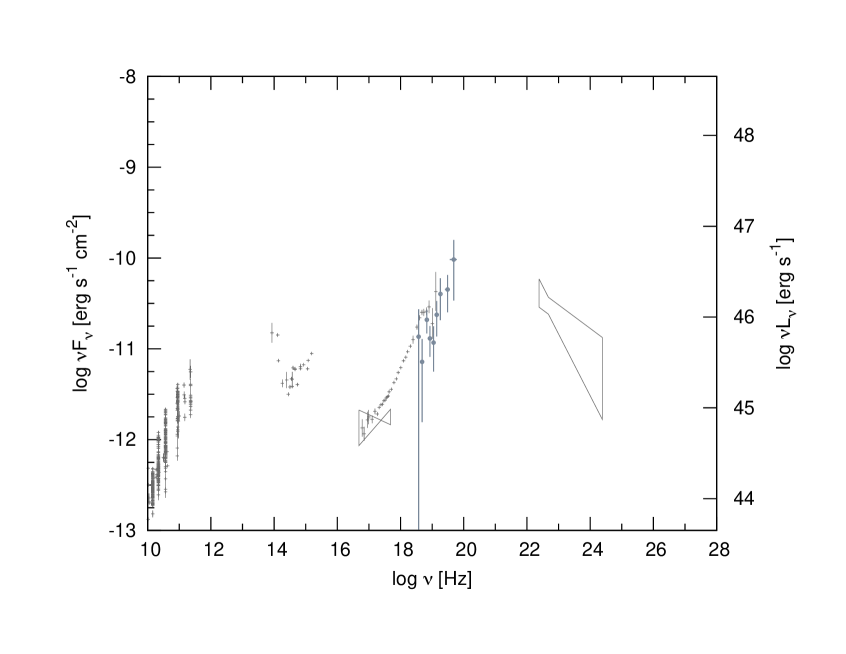
Figure 2.3: The archival data of PKS 1510-089 published by Kataoka et al. (2008), and the INTEGRAL observations (Barnacka & Moderski, 2009).

The multi-wavelength light curve is presented in figure 2.4.

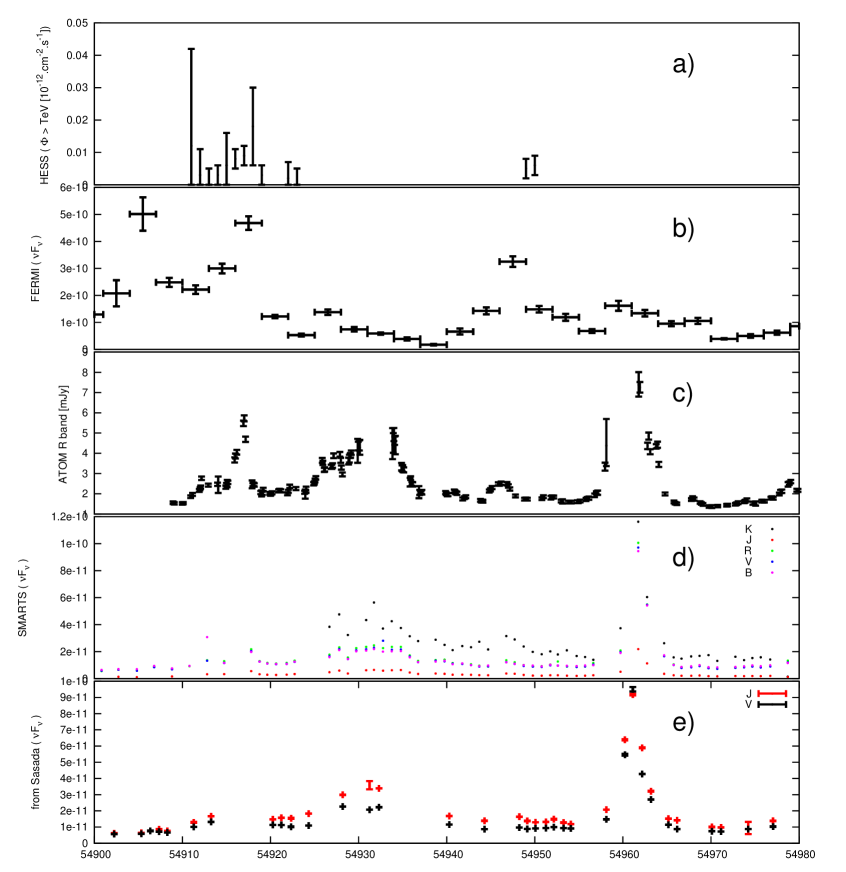
Figure 2.4: The multi-wavelength light curves of PKS 1510-211 during March - April 2009. a) The VHE light curve recorded by H.E.S.S. b) The HE energy observations carried out by FERMI LAT, shown in three-days bins. c) The ATOM R-band fluxes after correction for the Galactic absorption. d) Data taken with SMARTS: K,J,R,V,B filters (data were downloaded from http://www.astro.yale.edu/smarts/fermi/). e) The optical observations obtained using filters J and V (data taken from Sasada et al. (2011)).

2.15.1 H.E.S.S. data analysis

The observations with the H.E.S.S. telescope followed the report of flaring activities in HE (D’Ammando et al., 2009) and in the optical band observed by ATOM. The H.E.S.S. data were simultaneous with the peak of the HE flare recorded by FERMI. The H.E.S.S. telescopes carried out observations of PKS 1510-089 at two periods. The first observations were taken between 23 March 2009 (MJD 54910) and 2 April 2009 (MJD 54923). The second follow-up of the HE activity triggered the H.E.S.S. observations between 27 April 2009 (MJD 54948) and 29 April 2009 (MJD 54950). The H.E.S.S. observations resulted in 15.8 hours of good quality data.

The data quality selection is based on various variables like the trigger rate, the telescope tracking or the fraction of the PMTs turned off. Runs with the mean trigger rate less than 70% of the predicted value (Funk et al., 2005) are rejected. The mean system rate is 240 Hz for the four telescope data, and 180 Hz for the three telescope data. In addition, if the rms variation in the trigger rate is above 10%, the runs also are rejected. The instability of trigger rate can be caused by the presence of clouds or excessive dust in the atmosphere, which leads to the Cherenkov light absorption, and thus to the fluctuation in the trigger system efficiency.

The problems with telescope tracking can lead to errors in the reconstructed position of the source and thus can affect the flux. Runs with the tracking error problems reported by the DAQ are then rejected, when the rms deviations are greater than 10 arcseconds in altitude or azimuth.

An alternative check of the tracking system is performed by producing an intensity map of light of bright stars in the telescope field of view. The positions of known stars are then correlated with this map, giving a measure of the pointing position of each telescope. Runs are rejected, if the pointing deviation is greater than 0.1^∘.

Runs with more than 10% of the PMTs missing are rejected from the analysis. PMTs can be turned off, if any bright transient light source passes through it. Such a source of light can be bright stars, meteorites, lightening, airplanes or even satellites. Detail criteria of quality cuts are described in Aharonian et al. (2006).

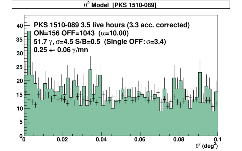
Figure 2.5: The angular distribution of events around the nominal position of PKS 1510-089. $\theta^{2}$ is the square of the angular distance between the nominal source position and the reconstructed arrival direction of an event.

The H.E.S.S. data analysis has been performed using the Model Analysis developped by de Naurois & Rolland (2009). Events were reconstructed using loose cuts appropriate for sources with steep spectra. PKS 1510-089 is a high redshift source, therefore its spectrum is expected to be soft due to the EBL absorption.

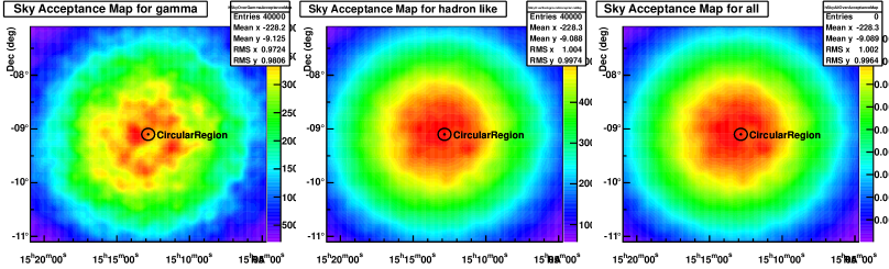
Figure 2.6: The camera response for $\gamma$-like (left panel), hadron-like (middle panel) and all (right panel) events, over the field of view (angular acceptance).

The analysis of the first flare (MJD 54916-54917), based on 3.5 hours of observations, recorded 51.7 photons from the source direction. This corresponds to a detection significance of 4.5 $\sigma$, following the method of Li & Ma (1983). The angular distribution of events around the position of PKS 1510-089 (figure 2.5) shows the excess in the source region. The acceptance distribution suffers from the low statistic of $\gamma$-like events, leading to an apparent inhomogeneity. The observed off-set in the $\theta^{2}$ distribution (figure 2.5) is due to problems with the pointing model. A new DST production with a better pointing correction is undergoing, however the pointing problem does not influence significantly the detection significance or the energy spectrum, since the whole excess in the $\theta^{2}$ distribution is within 0.1^∘ from the target.

The spectrum was derived using a forward-folding technique. The threshold energy, $E_{thr}$, is given by the energy at which the effective area falls to 10% of its maximum value. For these observations the energy threshold was estimated to be $E_{thr}\sim$ 0.15 TeV.

Most of the VHE events were detected below $\sim$ 400 GeV. The spectrum (figure 2.7) is fitted with a Power-Law: $dN/dE=N_{0}(E/E_{0})^{-\Gamma}$, with an index $\Gamma=9.8\pm 2.9$ and a normalization $N_{0}=(6.32\pm 0.35)\times 10^{-14}\,$m${}^{-2}\,$s${}^{-1}\,$TeV^-1 at $E_{0}$=157 GeV. The equivalent $\chi^{2}is7.8/13$ndf.

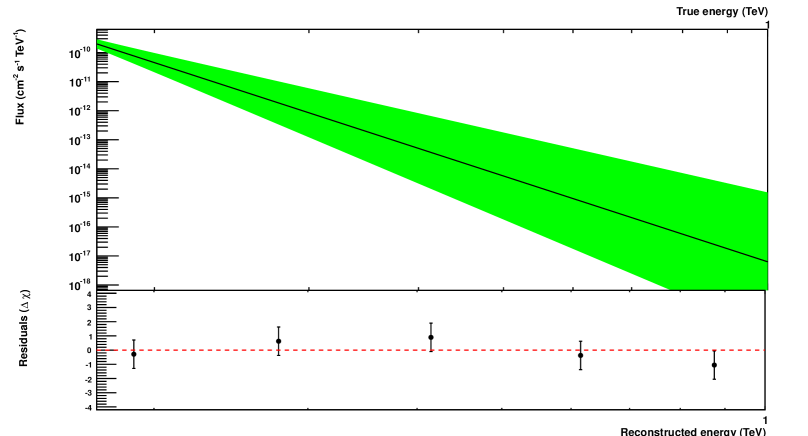
Figure 2.7: The VHE spectrum of PKS 1510-089 measured with the H.E.S.S. instrument, during March 2009. The solid line is the best-fit Power Law obtained using forward folding. The ”butterfly” is the 68% confidence band, while the points with errorbars (1$\sigma$ statistical errors) are the residuals in binned energy. Vectors denote the 99% C.L. upper limits.

2.15.2 FERMI data analysis

The Fermi-LAT (Atwood et al., 2009) data, simultaneous with the H.E.S.S. observations period, were analyzed using the publicly available Fermi Science Tools (version v9r15p2) and the P6_V3_DIFFUSE instrument response functions. The light curve (figure 2.4, b) is produced by an unbinned likelihood analysis taking into account photons (the diffuse class events) with energies between 200 MeV and 100 GeV from a region of interest (ROI) with a radius of 20^∘ around the position of PKS 1510-089. All sources, from the Fermi-LAT First Source Catalog (Abdo et al., 2010c), within an angular distance of 25^∘ PKS 1510-089, were modeled simultaneously. Model v02 of the Galactic and extragalactic backgrounds were used. Two flares are evident on the light curve (figure 2.4,b), one centered around MJD 54916, and the second centered around MJD 54948.

Figure 2.8 shows the LAT SED of PKS 1510-089 extracted for the flare observed around MJD 54916. Three different models have been fitted to the data: a Power Law, a Broken Power Law and an exponentially cut-off Power Law (ExpCut-off) model. Table 2.3 summarizes the values of the fitted parameters for all 3 models. The spectrum is best fitted by the ExpCut-off model, with an index of $-2.02\pm 0.1$, a break energy of 400 MeV and P1=$7.9\pm 4.5$. The flux obtained using the ExpCut-off model is $5.04\times 10^{-6}$ph cm^-2s^-1. The result of the fit is compatible with the one obtained by Abdo et al. (2010a).

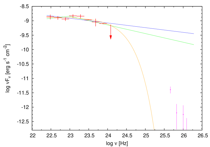
Figure 2.8: The HE spectrum of PKS 1510-089 observed with the FERMI LAT, during VHE flare on March 2009. The red points are the FERMI data and the magenta points are the H.E.S.S. data for comparison. The blue line represents the Power Law fit to the FERMI data, the green line is the Broken Power Law fit and the orange line is the exponentially cut-off power law (Exp Cut-off) fit. The values of the parameters obtained by fitting the models are summarized in table 2.3.

Model	Parameters
Power Law	Integral: $828.2\pm 60.7$, Index: $-2.16\pm 0.06$,
	Lower Limit: 100, Upper Limit: 10000,
	Npred: 305.551, ROI distance: 5.76807e-05,
	TS value: 1290.37
Broken Power Law	Prefactor: $5.64\pm 4.45(1e-09)$, Index1: $-1.85\pm 0.16$,
	Index2: $-2.3\pm 0.11$, Break Value:$399.7\pm 156$, [MeV]
	Npred: 304.527, ROI distance: 5.76807e-05,
	TS value: 1292.73,
Exp Cut-Off	Prefactor: $3.09\pm 2.4(1e-08)$, Index: $-2.02\pm 0.1$,
	Scale: $163\pm 62$, Ebreak: $400.4\pm 65$,
	P1: $7.9\pm 4.5(*1000)$, Npred: 304.878,
	ROI distance: 5.76807e-05,
	TS value: 1293.67,

Table 2.3: Results of the unbinned likelihood spectral fit of the flare of PKS 1510-089 (FERMI LAT data). The description of the spectral models can be found on page http://fermi.gsfc.nasa.gov/ssc/data/analysis/scitools/source_models.html. $Npred$ is the number of photons used in the fit. TS value is the Test Statistic resulting from the fit (Mattox et al., 1996). The region of interest (ROI) distance indicates the angular separation between the center of the ROI and the location of the fit for that source.

2.16 Modeling

I have aimed to reproduce the spectrum energy distribution (SED) of PKS 1510-089 during the HE and VHE flare recorded on March 2009. The approach was to use the one zone leptonic model implemented in the BLAZAR code (Moderski et al., 2003). The BLAZAR code requires some input parameters, notably the value of the energy density of an external diffuse radiation field, the injected electron energy distribution, the value of the magnetic field and the description of the overall geometry of the source.

In this work I consider two sources of the external photons: DT and BLR. The luminosity of the accretion disk has been reported by Nalewajko et al. (2012) to be $L_{d}=5\times 10^{45}\,\mbox{erg\, s}^{-1}$. Following equation (2.3), the size of the BLR, $r_{BLR}$, is estimated to be $0.12\times 10^{18}\,$cm. The size of the DT is approximatively by $r_{DT}\simeq 1.94\times 10^{18}\,$cm (see section 2.6).

The energy density of external radiation fields have been calculated using equations (2.8) and (2.4). To satisfy the physical boundaries on the fraction of reprocessed emission from the accretion disk, I have used $\xi_{BEL}\sim 0.1$ and $\xi_{BEL}\sim 0.2$. The values of $\xi_{BEL,DT}$ together with values of $L_{d},\,r_{BEL,DT}$ listed above, and taking into account the dust temperature $T_{3}=1.8$ from Nalewajko et al. (2012), one can get the energy density of external radiation fields: $u_{BEL}=0.09\,{\rm erg\,cm^{-3}}$ and $u_{DT}=0.0005\,{\rm erg\,cm^{-3}}$. The jet opening angle, $\theta_{\rm jet}$ is assumed to be $1/\Gamma$.

Table 2.4: The input parameters for modeling of the non-thermal emission of PKS 1510$-$089.

Parameter	Model
minimum electron Lorentz factor $\gamma_{\rm min}$	$1$
break electron Lorentz factor $\gamma_{\rm br}$	$900$
maximum electron Lorentz factor $\gamma_{\rm max}$	$10^{5}$
low-energy electron spectral index $p$	$1.2$
high-energy electron spectral index $q$	$3.5$
normalization of the injection function $K_{e}$	$2.0\times 10^{46}\,{\rm s^{-1}}$
bulk Lorentz factor of the emitting plasma $\Gamma_{\rm jet}$	$22$
jet opening angle $\theta_{\rm jet}$	$0.045$ rad
jet viewing angle $\theta_{\rm obs}$	$0.045$ rad
location of the blazar zone $R_{\rm 0}$	$0.7\times 10^{18}$ cm
jet magnetic field intensity $B$	$0.75$ G
scale of the BEL external photon field $r_{\rm BEL}$	$0.12\times 10^{18}$ cm
energy density of the external photon field $u_{\rm BEL}$	$0.09\,{\rm erg\,cm^{-3}}$
photon energy of the external photon field $h\nu_{\rm BEL}$	$10$ eV
scale of the DT external photon field $r_{\rm DT}$	$1.94\times 10^{18}$ cm
energy density of the external photon field $u_{\rm DT}$	$0.0005\,{\rm erg\,cm^{-3}}$
photon energy of the external photon field $h\nu_{\rm DT}$	$0.15$ eV

The other parameters are estimated to best reproduce the observed multi-wavelength spectrum of PKS 1510-089. The parameters are summarized in table 2.4, while the spectrum obtained is presented in figure 2.14.

The BLAZAR code calculates the evolution of electrons injected along the jet. Figure 2.9 shows the electron evolution during the flare of PKS 1510-089. The injected electrons follow a broken power law distribution (see equation 2.15). Parameters of the electron injection function are listed on table 2.4. The electron injection starts at $R_{0}$ and continues until $R=2R_{0}$, while the electron evolution is followed up to 3$R_{0}$. The proper choice of $R_{0}$ is crucial for the SED modelling. The next section is dedicated to the discussion of the location of the blazar zone in PKS 1510-089.

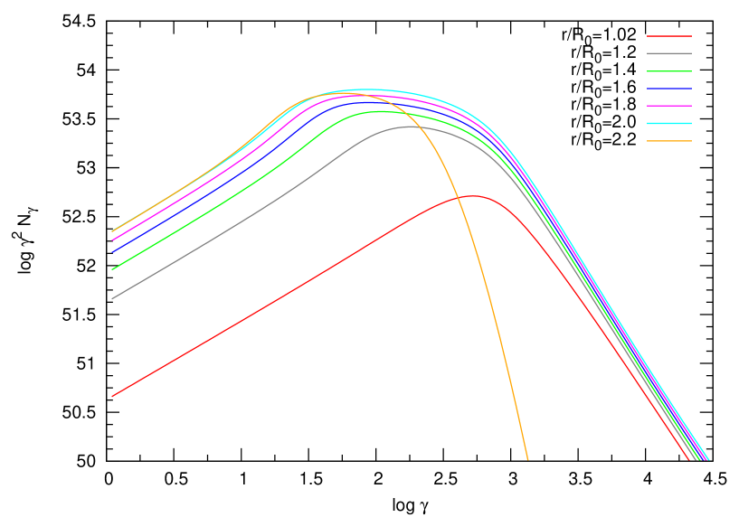
Figure 2.9: Evolution of the electron energy distribution during the March 2009 flare of the blazar PKS 1510-089. The evolution is calculated using the BLAZAR code and model parameters taken from table 2.4.

2.16.1 Location of the $\gamma$-ray emitting region in PKS 1510-089

The choice of the distance of the shock formation from the central source, $R_{0}$, is constrained from one side by the internal absorption of gamma rays in BLR, and from the other side by the IC efficiency. Figure 2.10 shows the internal absorption, $e^{-\tau}$, as a function of the photon energy emitted at different $R_{0}$. When $R_{0}$ is below $r_{BLR}$ then a significant fraction of the HE radiation (from a several dozen to several hundred GeV) is absorbed. If $R_{0}$ is greater than $r_{BLR}$ then only a few percent of the HE emission is absorbed.

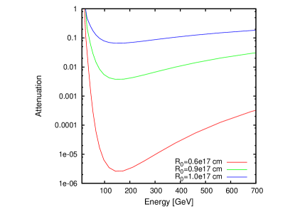
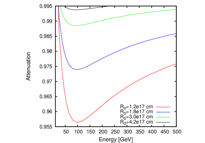
Figure 2.10: The internal absorption as a function of photon energy emitted in the blazar zone. The values of attenuation, $e^{-\tau}$, is calculated for different distances from the center and assuming PKS 1510-089 model parameters listed in table 2.4. Left panel: $R_{0}$ below $r_{BEL}$. Right panel: $R_{0}$ above $r_{BEL}$.

However, if the blazar zone is too far away from the BLR then the photon energy density is too small to produce a sufficient $\gamma$-ray emission by IC. The photon energy densities of different radiation fields are presented in figure 2.11.

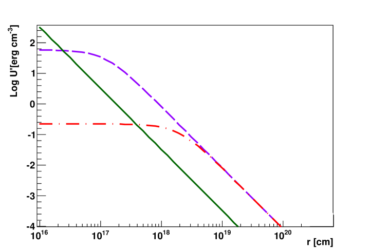
Figure 2.11: The energy density as a function of the distance from the central source, calculated using parameters listed in the table 2.4. The violet dashed line represents the energy density of BLR, the red dashed-dotted line shows the energy density of DT, and the green line is the energy density of magnetic field.

There exists some observational evidence that the blazar zone may be located outside the BLR. The radio observations of PKS 1510-089 between 2011 September 9 and 2011 October 17 (Marscher et al., 2010) show a $\sim$ 40 days ($\Delta t_{obs}$) increase in radio flux. If the $\gamma$-ray flare is indeed associated with the same region as the slower radio flare (Marscher et al., 2010; Orienti et al., 2012), the projected distance between the regions where the shock formed and the site responsible for the $\gamma$-ray emission is:

$$D_{projected}=\frac{\beta_{app}c\Delta t_{obs}}{(1+z)}=\frac{(25c\times 40\,\mbox{days})}{1.36}=0.6\,\mbox{pc}=1.8\times 10^{18}\,\mbox{cm}$$ (2.32)

where $\beta_{app}$ is the apparent velocity. One then finds that the $\gamma$-ray flare is produced at the projected distance of $\sim\,$0.6 pc from the site where the shock detected in the radio band was formed. Assuming a jet inclination angle of $\theta=3^{\circ}$ (Orienti et al., 2012; Marscher et al., 2010), the de-projected distance ($D_{de-projected}=D_{projected}/\sin{\theta}$) is about $\simeq$ 10 pc. This shows that at least for some $\gamma$-ray flares, the blazar zone may be located far outside the BLR.

In the presented modeling of PKS 1510-089, I adopted $R_{0}=0.7\times 10^{18}\,$cm. At that distance, the absorption by the low energy photons originating from the BLR, is very small, of the order of 1%, while the energy density (see figure 2.11) in the blazar zone of PKS 1510-089 ($0.7-1.4\times 10^{18}\,$cm) is still dominated by radiation from the BLR. Outside $r_{BLR}$, the external radiation field is dominated by $u_{BEL}$ up to a distance $r_{DT}$, where $u_{BEL}$ became comparable to the energy density of the radiation from DT ($u_{DT}$).

2.16.2 Spectral energy distribution

Figure 2.12 presents the Klein-Nishina (KN) correction ($\sigma_{KN}/\sigma_{T}$) as a function of energy for different electron Lorentz factors $\gamma$. The KN correction is presented together with the radiation of BLR and DT approximated as black body. For small $\gamma$, electrons cool in the Thomson regime. The electrons with Lorentz factors above $10^{3}$ are responsible for the HE and VHE emissions.

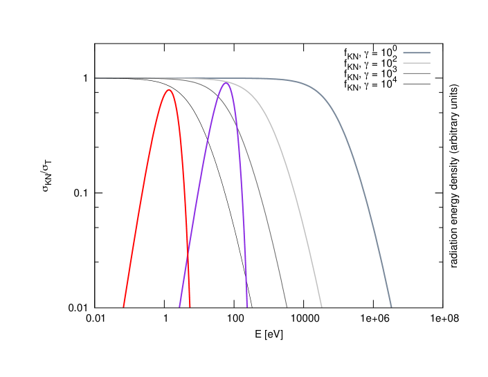
Figure 2.12: The $f_{KN}$ correction (see equation (2.24)) at different electron Lorentz factors $\gamma$ (gray lines). $f_{KN}$ is expressed as a fraction of Thomson cross-secton ($\sigma_{KN}/\sigma_{T}$). The violet and red lines represent the energy densities of two external photon fields: BLR and DT, respectively. The energy density is approximated by a black body distribution with characteristic frequency in the comoving frame $\nu^{\prime}=\Gamma\nu$, and the corresponding energy density seen in comoving frame is approximated as $u^{\prime}=4/3\Gamma^{2}u_{ext}$. The photon densities for corresponding external photon fields were calculated using values listed in table 2.4.

The rate of IC energy losses of relativistic electrons, calculated using equation (2.21) is shown on figure 2.13. The external photon energy densities in the region located at $R_{0}$ to $2R_{0}$ shows that the energy density of the BLR exceeds a few times the energy density of DT (see figure 2.13). However, the electron cooling, in this region is faster for seed photons originating from DT. Therefore, despite of the greater energy density of BLR over DT, the last one is responsible of the VHE photon production via IC radiation.

All above arguments suggest the following scenario for the PKS 1510-089 flaring activity recorded on March 2010:

• The low energy component is produced by the synchrotron radiation.

• The high energy component (from X-rays to VHE) is produced by two components:

• The first component is the IC radiation with seed photons from the BLR. This component dominates the emission in the FERMI range. Due to the KN effect this component alone cannot explain the highest part of the spectrum ($>$100 GeV).

• The VHE emission is produced via IC scattering of the seed photons originating from DT. The same component is also responsible for the X-ray part of the spectrum, as in the previous modeling attempts of this object (Kataoka et al., 2008).

• The modeled emission of PKS 1510-089 convolved with the EBL attenuation, calculated using Spitzer constraints on the EBL (Dole et al., 2006), fits well all the observations.

Figure 2.14 shows the result of the modelling of the PKS 1510-089 during the flare.

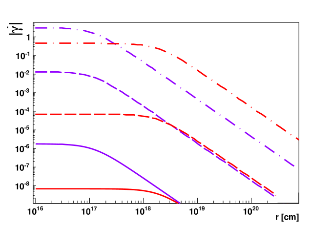
Figure 2.13: The rate of IC energy losses of relativistic electrons calculated using equation (2.21). The IC cooling is presented for two sources of seed photons: BLR (violet lines) and DT (red lines). The cooling rate was calculated for different electron Lorentz factors $\gamma$: 1 (solid lines), 100 (dashed lines), 10000 (dashed-dotted lines).

2.17 Discussion

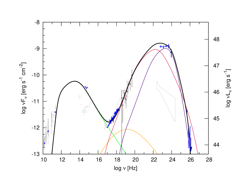
Figure 2.14: The overall spectrum of the PKS 1510-089. The green line represents the synchrotron component, the red line is IC component with seed photons originating from DT before absorption, and the violet line is IC radiation with seed photons originating from BLR. The orange line is the SSC component. The black line represents the sum of the all components, corrected for EBL absorption (Spitzer model) and absorption on the low energy photons originating from BLR and DT.

The most recent attempt of PKS 1510-089 modeling was undertaken by Nalewajko et al. (2012), who analyzed the 2011 low state of of the object. They used the data obtained with the Herschel satellite to constrain the theoretical models. Nalewajko et al. (2012) concluded that a multi-zone emission model is necessary to explain the spectral properties of PKS 1510-089. The model of Nalewajko et al. (2012) differs from the model proposed by Abdo et al. (2010a), who analyzed the object in 2009 during an active state. The fast optical flares observed in 2009 were significantly brighter and strongly polarized as compared to those observed in 2011.

The optical flaring activity in 2009 was maybe accompanied by an increase of the magnetic field. This is confirmed by the observation of the significant increase in the optical degree of polarization (Sasada et al., 2011) and observations of the superluminal knot with VLBA at 7 mm (Marscher et al., 2010). This behavior of the low energy component was not observed in 2011 when Herschel data were taken.

PKS 1510-089 was detected with the H.E.S.S. system on March – April 2009 during the high state in the HE and optical domains. Abdo et al. (2010a) model the emission for energies below 100 GeV, without predictions for the VHE emission. In this thesis, I developed a single zone model to explain the emission of PKS 1510-089 during the flare observed on March 2009, where the emission of the low energy component is produced by the synchrotron radiation and the high energy component is produced by the same population of ultra-relativistic electrons via an IC process.

2.18 Conclusions

I have successfully modeled PKS 1510-089 with the single zone internal shock scenario. It has been confirmed that the IC BLR cannot explain the VHE emission due to the KN effect, as was anticipated by Moderski et al. (2005).

The observations of PKS 1510-089 with the H.E.S.S. array show a VHE emission up to 400 GeV. The observations during the flare provide a 4.5 $\sigma$ detection of this emission.

The absorption of the HE and the VHE photons in the blazar itself has been also investigated. The absorption in the BLR is avoided by locating the blazar zone outside the BLR. The absorption by photons from DT and EBL absorption become significant only for photons with energies above 400 GeV. This emission was not observed in the case of PKS 1510-089.

Marscher et al. (2010) demonstrated that the HE emission from the jet of PKS 1510-089 is quit complex. The emission arises from different regions and probably multiple emission mechanisms are involved. I have tried to explain the emission of PKS 1510-089 during the flare on March 2009. The peak luminosity of the low energy component during the flare was much higher than that of observations shown by Nalewajko et al. (2012).

The VHE emission can be a very common feature of FSRQs. The H.E.S.S. II telescope, with its energy range from tens of GeV, will provide a great opportunity to search for emission from other objects of this class.

Part III Theory of Gravitational Lensing

3.1 Introduction

The lensing phenomena is an important topic in the cosmology. Parts IV and V of my thesis shows two examples of the lensing phenomena studied at high energy range. The first study (part IV) provides the method of the time delay estimation when the lens images are spatially unresolved. Then, in the last section of part IV, I have showed the application of the obtained time delay to the Hubble constant estimation. The second study (part V) presents the limits on the abundance of compact objects. The limits have been obtained searching for femtolensing effect in the spectra of GRBs. The follow part of the thesis provide a brief theoretical introduction concerning parts IV and V.

3.2 Gravitational Lensing

Gravitational lensing observations can be divided into strong, weak and micro-lenses. These lenses have different masses and image characteristics.

Strong lensing events have multiple resolved images and arcs or arclets. They are produced by the lensing of a distant object by galaxies or clusters of galaxies.

The weak lensing is a regime where background galaxies are slightly distorted by foreground masses. Weak gravitational lensing can thus be detected by studying the morphology of a large number of galaxies. It is therefore, an intrinsically statistical measurement.

A large part of the lensing observations is dedicated to microlensing. In the case of microlensing, the lenses have stellar masses. The images separation and time delay are too small to be detected. However, the characteristic time dependent magnification pattern helps to distinguish the microlensing event from the intrinsic variability of lensed sources. The analysis of the light curve of a microlensed source can provide informations on the nature of the lens. The lensing event time scale is a combination of the lens mass, the transverse velocity, and the distances between the lens, the source and the observer.

Applications of gravitational lensing include:

• Cosmology (Hubble constant (Suyu et al., 2010), compact objects (Press & Gunn, 1973; Tisserand et al., 2007), $\sigma_{8}$ (Dahle, 2006))

• Astrophysics (Mao, 2012)(stellar atmospheres (Thurl et al., 2004), extrasolar planets, galactic structure, mass estimates)

• Fundamental physics (post Newtonian parameters(Bolton et al., 2006))

This thesis is focusing on two different lensing phenomena. The first one is strong gravitational lensing and the other described in the thesis, similar to microlensing, is called femtolensing.

3.3 Theory

The gravitational lensing effect arises when a concentrated mass (”lens”) lies in the line of sight from the observer on the Earth to a distant object (”source”), see figure 3.1. The lensing effect magnifies and distorts the image of the source. Depending on the geometry of the lens, the resulting image of the lensed object might be an arc, a complete ring, a series of multiple images or a combination of compact images and arcs (see e.g. review by Blandford & Narayan (1992)).

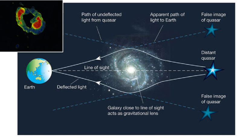
Figure 3.1: Schematic view of a gravitationally lensed system.

The deflection of photons in the presence of masses is a consequence of the principle of equivalence. The first correct formula for the deflection angle $\alpha$ was derived by Einstein. The deflection angle $\alpha$ of light passing at the distance $r$ from an object of mass $M$ is given by equation:

$$\alpha=\frac{4GM(r)}{c^{2}}\frac{1}{r}\,.$$ (3.1)

Equation (3.1) gives a deflection angle twice larger than the Newtonian deflection for a slow particle. The light deflection angle by the Sun is:

$$\alpha=\frac{4GM_{\odot}}{c^{2}}\frac{1}{R_{\odot}}=1.74\,\mbox{arcsec}\,.$$ (3.2)

The deflection angle was first measured by Eddington during a solar total eclipse. The Eddington experiment in 1919 brought the first experimental confirmation of the Einstein predictions concerning light deflection.

However, observing the lensing of stars by stars was at that time considered as technologically impossible due to the very small image separation of the microlensed event. Fritz Zwicky (1937b, a) was the first to point out that galaxies are likely to be gravitationally lensed and the image separation would be detectable.

The angular separation of images in galaxy or galaxy cluster lensing is usually of the order of a few arcseconds. A typical galaxy with a mass of $1.25\times 10^{9}\,$ M_⊙ acting as a lens will produce an Einstein ring with an angular size of $\sim 0.5\,$arcsecond. A galaxy cluster at $z_{L}$=0.7 lensing a source at $z_{S}$=2 will lead to image separation of the order of 50 arcseconds.

3.3.1 Lens Equation

Gravitationally lensed systems involve a source, a lens and an observer, as shown on figure 3.2. A light ray from the source is deflected by an angle $\alpha$ by the lens and reaches the observer. Figure 3.2 shows the corresponding angular and linear distances in a typical gravitationally lensed system. The projected distance from the true source position to the lens is $r_{S}$ (in the lens plane). $D_{OL}$ and $D_{LS}$ are respectively the angular diameter distances between the observer and the source, and the observer and the lens (see section 3.4.1). The lens is assumed to be point like, thus the light rays emitted by the source are splitted into two images $r_{+}$ and $r_{-}$.

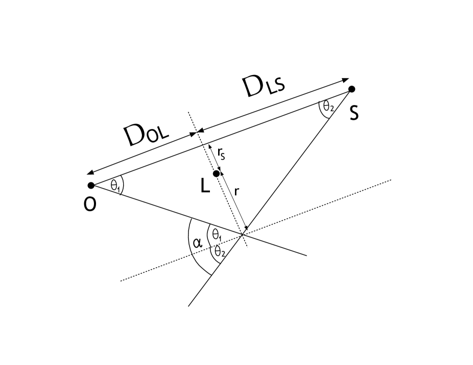
Figure 3.2: Geometry of a lensing event. The angles and angular diameter distances are shown. The light ray propagates from the source to the observer and passes the lens at distance $r_{S}$ in the lens plane. The angular diameter distances between the observer and the source, the observer and the lens are $D_{OL}$, and $D_{LS}$, respectively.

For $\theta_{1}$,$\theta_{2}$,$\alpha\,\ll$ 1 and $r_{S}<0$, figure 3.2 shows the following relations:

$$\theta_{1}=\frac{r-r_{S}}{D_{OL}}\,,$$ (3.3)

$$\theta_{2}=\frac{r-r_{S}}{D_{LS}}\,,$$ (3.4)

$$\theta_{1}+\theta_{2}=\alpha\,.$$ (3.5)

The angle $\alpha$ is known from equation 3.1. After simple transformations:

$$(r-r_{S})\left(\frac{1}{D_{OL}}+\frac{1}{D_{LS}}\right)=\frac{4GM}{c^{2}}\frac{1}{r}\,.$$ (3.6)

Equation (3.6) has one solution when the source and the lens are perfectly aligned ($r_{S}=0$). The image in the source plane is a ring around the lens with radius:

$$r_{E}^{2}=\frac{4GM}{c^{2}}\frac{D_{LS}D_{OL}}{D_{OS}}\,,$$ (3.7)

$r_{E}$ (equation (3.7)) is called the Einstein Radius.

For a point lens and $r_{S}\neq 0$, the lens equation (3.6) has two solutions. The first solution gives a distance between the first image and the lens:

$$r_{+}=\frac{1}{2}(r_{S}+\sqrt{r_{S}^{2}+4r_{E}^{2}})\,,$$ (3.8)

and accordingly a distance between the second image and the lens of:

$$r_{-}=\frac{1}{2}(r_{S}-\sqrt{r_{S}^{2}+4r_{E}^{2}})\,.$$ (3.9)

For an isolated point source, the solution of the lens equation always gives two images of a background source, with corresponding positions $r_{+}$ and $r_{-}$.

The lensing regime is based on the size of the image separation. The angular radius of the Einstein ring is given by:

$$\theta_{E}=\frac{r_{E}}{D_{OL}}=\sqrt{\frac{4GM}{c^{2}}\frac{D_{LS}}{D_{OL}D_{OS}}}\,.$$ (3.10)

If one considers the lensing of a source by a galaxy at a cosmological distance of $D\sim$ 1 Gpc and with mass $M\sim 10^{11}$ M_⊙ the corresponding Einstein angle is

$$\theta_{E}=0.9\left(\frac{M}{10^{11}M_{\bigodot}}\right)^{\frac{1}{2}}\left(\frac{D}{\mbox{Gpc}}\right)^{-\frac{1}{2}}\mbox{arcsec}\,.$$ (3.11)

Image separations of the order of arcseconds can be easily spatially resolved with optical and radio telescopes. The situation is much different when the lens is an object with a stellar mass or smaller. To illustrate this, the lensing by a star (with a mass M_⊙), in the Galaxy at a distance of D $\sim$ 10 kpc will produce an Einstein angle of the order of a miliarcsecond:

$$\theta_{E}=0.9\,\left(\frac{M}{M_{\bigodot}}\right)^{\frac{1}{2}}\left(\frac{D}{10\,\mbox{kpc}}\right)^{-\frac{1}{2}}\mbox{milliarcsec}.$$ (3.12)

When the image separation is of the order of one milliarcsecond, the lensing event is called a microlens. When the image separation is of the order of a femtoarcsecond, the effect is called femtolensing. For instance, when the distance of the lens is cosmological and the mass of the lens is in the range $10^{17}$ - $10^{20}\,$g, one gets:

$$\theta_{E}=0.3\,\left(\frac{M}{10^{17}\,\mbox{g}}\right)^{\frac{1}{2}}\left(\frac{D}{\mbox{Gpc}}\right)^{-\frac{1}{2}}\mbox{femtoarcsec\,}.$$ (3.13)

Objects like primordial black holes or axions clusters are in the mass range relevant to femtolensing.

3.3.2 Time delay

When multiple images of a source are resolved, their light curves are similar except for a shift in time. The shift in time comes from the differences in the geometrical path of light and the gravitational potential felt by the photon for each individual image. Estimation of this time delay, together with the measurements of the brightness ratio of individual images are crucial for determining the parameters of the lens, such as the lens mass and geometry. The time delay $\delta t$ between the two images (see figure 3.3) is given by

$$c\delta t=V(r_{+};r_{S})-V(r_{-};r_{S})\,,$$ (3.14)

where $V(r;r_{S})$ is the Fermat potential at the position $r$ in the lens plane.

$$V(r;r_{S})=\frac{1}{2}\frac{D_{OS}}{D_{LS}D_{OL}}(r-r_{s})^{2}-\frac{4GM}{c^{2}}ln(r)\,.$$ (3.15)

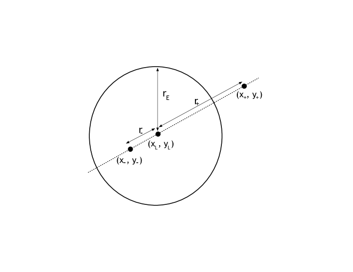
Figure 3.3: Definition of distances in the lens plane.

One finds:

$$\frac{c\delta t}{(z_{L}+1)}=\frac{c(\delta t_{geom}+\delta t_{grav})}{(z_{L}+1)}=\frac{1}{2}\left(\frac{D_{OS}}{D_{OL}D_{LS}}\right)(r_{-}^{2}-r_{+}^{2})-\frac{4GM}{c^{2}}\ln\left(\frac{r_{+}}{r_{-}}\right)\,.$$ (3.16)

The time delay $\delta t$ is a function of the image geometry, the distances $D_{OL}$, $D_{LS}$ and the gravitational potential. The geometrical time delay $\delta t_{geom}$ is caused by the extra path length compared to the direct line between the observer and the source. The gravitational time delay $\delta t_{grav}$ called the Shapiro delay (Shapiro 1964), is induced by the gravitational potential of the lens. The Shapiro effect is due to clocks slowing down in gravitational fields. Light rays are thus delayed relative to their travel time in vacuum.

The Fermat potential (equation (3.15)) can also be used to derive the lens equation by searching for extrema of the travel time:

$$\frac{dV}{dr}=0\,,$$ (3.17)

which gives:

$$(r-r_{S})\left(\frac{1}{D_{OL}}+\frac{1}{D_{LS}}\right)=\frac{4GM}{c^{2}}\frac{1}{r}\,.$$ (3.18)

Equation (3.18) is similar to (3.6).

3.3.3 Magnification

The magnification of a single image of a lensed system is the ratio of the flux of the image to the flux of the unlensed source. If there are several images, the magnifications add up.

In the case of a point mass lens, the amplitude contributed by the $r_{\pm}$ images is

$$A_{\pm}\propto\frac{\exp(i\phi_{\pm})}{\sqrt{|1-\frac{r_{E}^{4}}{r_{\pm}^{4}}|}}\,.$$ (3.19)

The magnification $|A|^{2}$ is obtained by summing the amplitudes (3.19) and squaring, which gives

$$|A|^{2} = |A_{+}+A_{-}|^{2}=$$ (3.20)

$$= \frac{1}{1-\frac{r_{E}^{4}}{r_{+}^{4}}}+\frac{1}{1-\frac{r_{E}^{4}}{r_{-}^{4}}}+\frac{2\cos(\Delta\phi)}{\sqrt{|1-\frac{r_{E}^{4}}{r_{+}^{4}}|}\sqrt{|1-\frac{r_{E}^{4}}{r_{-}^{4}}|}}\,.$$

The phase difference $\Delta\phi$ is given by equation:

$$\Delta\phi=\frac{E\delta t}{\hbar}\,.$$ (3.21)

When light is not coherent ($\Delta\phi\gg 1$), the equation (3.20) is reduced to the two first terms. If one considers a ”traditional” lensing event (such as microlensing), the two light paths are not coherent because of large time difference between the images: $\lambda/c\ll\delta t$. This is essentially the geometric optics approximation. However, the condition of light coherence can be fulfilled, when the lensing object is very small and compact. In that case, the induced time difference between images is comparable to the light wavelength. When light is coherent, fringes can be observed in the energy spectrum. This interferometry pattern may be observed in GRB spectra if a compact object is on the line of sight with mass in the range $10^{14}\,g\,-\,10^{19}\,g$. The GRBs emits mostly in the energy range from ${\rm keV}$ to ${\rm MeV}$. The condition of coherence ($\Delta\phi~{}\sim~{}\left(E/1{\rm MeV}\right)\left(M/1.5\times 10^{17}\,{\rm g}\right)$ close to 1) can thus be satisfied. This idea was proposed first by Gould (1992), who also invented the word ”femtolensing”.

3.3.4 Projected size of a source

In principle, the finite size of the source and the relative motion of the observer, the lens and the source have to be taken into account. In this thesis this effects are important only for GRBs femtolensing. The projected size effect is negligible provided $s_{GRB}/r_{E}$ is $\ll$ 1, where $s_{GRB}$ is the size of GRB emission region projected on the lens plane. If the GRB is observed at a time $t_{expl}$ after the beginning of the burst, its size projected onto the lens plane is

$$s_{GRB}\approx\frac{D_{OL}}{D_{OS}}\frac{ct_{expl}}{\Gamma}\\ \approx\left(c\times 0.01\,\mbox{s}\right)\,\left(\frac{t_{expl}}{1\,\mbox{s}}\right)\left(\frac{\Gamma}{100}\right)^{-1}\left(\frac{D_{OL}}{D_{OS}}\right)\,,$$ (3.22)

where $\Gamma$ is the Lorentz factor of the burst. Note that the Lorentz factor of GRBs is estimated to be in excess of $100$, so that $s_{GRB}$ given in equation (3.22) is overestimated.

The Einstein radius $r_{E}$, image position and time delay have been introduced in section 3.3.1. The Einstein radius for the femtolensing event is of the order of:

$$r_{E}^{2}=\frac{4GM}{c^{2}}\frac{D_{OL}D_{LS}}{D_{OS}}\\ \approx{\left(c\times 0.3\,\mbox{s}\right)}^{2}\left(\frac{D_{OL}D_{LS}}{D_{OS}\,1\,\mbox{Gpc}}\right)\left(\frac{M}{10^{19}\,\mbox{g}}\right)\,,$$ (3.23)

The ratio of $s_{GRB}$ to $r_{E}$ is therefore

$$\frac{s_{GRB}}{r_{E}} \approx \frac{c^{2}}{2G^{1/2}}\frac{t_{expl}}{M^{1/2}\Gamma}\left(\frac{D_{OS}D_{LS}}{D_{OL}}\right)^{-1/2}$$ (3.24)

$$\approx 0.03\left(\frac{D_{OS}D_{LS}}{D_{OL}\,1\,\mbox{Gpc}}\right)^{-\frac{1}{2}}\left(\frac{t_{expl}}{1\,\mbox{s}}\right)\times\left(\frac{\Gamma}{100}\right)^{-1}\left(\frac{M}{10^{19}\,\mbox{g}}\right)^{-\frac{1}{2}}\,.$$

Equation (3.24) shows that the finite size of the GRB can be in general safely neglected if $t_{expl}<10\,\mbox{s}$.

3.3.5 Time scale of femtolensing events

The expected time scale femtolensing-induced event is given in terms of the typical Einstein radius and relative velocity $v$ between source and lens. The Einstein radius crossing time $t_{E}$ is then:

$$t_{E}=\frac{r_{E}}{v}\\ \approx 300\,\mbox{s}\,\left(\frac{r_{E}}{c\times 0.3\,\mbox{s}}\right)\left(\frac{v}{300\,\mbox{km/s}}\right)^{-1}\,.$$ (3.25)

Equation (3.25) shows that $t_{E}\gg t_{expl}$ under reasonable assumptions on the velocities. If so, the motion of the source in the lens plane can also be neglected. In the analysis of GRB spectra, it is thus assumed that the point source – point lens assumption is valid and that the source stays at a fixed position in the lens plane.

3.3.6 Singular Isothermal Sphere

Primordial black holes can be modeled as point lenses. However, galaxies which are responsible for large time delays between the images are extended lenses. A simple model of extended lenses is a singular isothermal sphere model (SIS). In this model, the mass increases proportionally to the radius $r$ and the force is proportional to $1/r$. Thus, the isothermal sphere is a first approximation model for the gravitational field of galaxies and cluster of galaxies (Rubin et al., 1988). The three-dimensional density distribution of SIS is given by:

$$\sigma=\frac{\nu^{2}}{2\pi G}\frac{1}{r^{2}}\,,$$ (3.26)

where $\nu$ is the one-dimensional velocity dispersion of stars in the galaxy.

The circularly-symmetric surface mass distribution is obtained by projecting the matter in the lens plane:

$$\Sigma(r)=\frac{\nu}{2G}\frac{1}{r}\,.$$ (3.27)

The mass inside a sphere of radius $r$ is given by

$$M(r)=\int_{0}^{r}\Sigma(r^{\prime})2\pi r^{\prime}dr^{\prime}\,.$$ (3.28)

Using equation (3.1) and (3.28) one obtains:

$$\alpha(r)=4\pi\frac{\nu^{2}}{c}\,.$$ (3.29)

Equation (3.29) shows that the deflection angle for an isothermal sphere is independent of $r$. Equation (3.29) can be simplified to:

$$\alpha=1.15\left(\frac{\sigma_{\nu}}{200\,km\,s^{-1}}\right)^{2}\,{\rm arcsec}\,.$$ (3.30)

The Einstein angle calculated in SIS model is:

$$\theta_{E}=4\pi\frac{\nu^{2}}{c^{2}}\frac{D_{LS}}{D_{OS}}=\alpha\frac{D_{LS}}{D_{OS}}\,.$$ (3.31)

SIS creates two images of the source if it lies inside the Einstein ring, else just one image. A third image is hidden by the central singularity of the $\ln(r)$ potential.

3.4 Lensing Probability

The chance of seeing a lensing event is usually expressed in terms of optical depth. This assumes that the optical depth is smaller than 1, so that it can be understood as a probability. The concept of optical depth was introduced by Vietri & Ostriker (1983), and is the standard way of determining the probability of lensing. The optical depth $\tau$ is defined, in the context of gravitational lensing, as a measure of the number of lenses per Einstein ring along the line of sight from the observer to a given source (Nemiroff, 1989). That is:

$$\tau=\int{\rho_{lens}\pi r_{E}^{2}dl}\,,$$ (3.32)

where $\rho_{lens}$ is the density of lenses along the line of sight.

The connection between the optical depth and the lensing probability depends on the observations and on the performances of the instrument. For instance in microlensing observations lenses are observed when the magnification is larger than 1.34, corresponding to one Einstein radius. Some of the current instruments like Kepler, can detect tiny magnitude variations, when sources are bright enough. In that case the lensing probability is obtained from the maximum area in the lens plane, where a passing source gives detectable lensing effects (Griest et al., 2011). In general it is convinient to define a lensing ”cross-section”, which reflects the maximum detectable area in the lens plane and depends on the lens observation method (see Schneider (1999) section 11.1),

The microlensing event detection is based on the observation of magnification changes of sources. In contrast, the detection of femtolensing is based on the observation of fringes in the energy spectrum (see figure 5.1). With GBM, the fringes can be detected when a lens is distant of more than 3 $r_{E}$ from the source. At this distance the magnification change is not detectable any more. In the case of femtolensing the cross-section has been defined as the area in the lens plane where the spectral fringes give a more than 3 sigma detection. The femtolensing cross-section depends on the instrument performance and source brightness, so that it was calculated event by event (see part V).

The optical depth is sensitive to the cosmological model. The Universe is homogeneous and isotropic at large scales and is well described by the Friedmann-Lemaitre-Robertson-Walker (FLRW) geometry. The FLRW is characterized by just a few parameters including the mean mass density $\Omega_{M}$ and the normalized cosmological constant $\Omega_{\Lambda}$. However, the local clumpiness has an important effect on photon propagation. This leads to different formula for the angular diameter distance.

In the next section 3.4.1 the various distance formula are described, then in sections 3.4.2 and 3.4.3 the formalism of the optical depth calculation for the point mass and SIS models is presented. I have followed the analysis of Fukugita et al. (1992).

3.4.1 The Distance Formula

Based on observations, the Universe is homogenous on large scales. Therefore, on large scales it is well approximated by the FLRW geometry. However, at smaller distances, the light propagates through an inhomogeneous space-time rather than the averaged smooth space-time. The light ray feels the local metric which deviates from the smoothed Robertson-Walker metric.

Even if global parameters like the mean mass density $\Omega_{M}$ and the normalized cosmological constant $\Omega_{\Lambda}$ are fixed, the propagation of light rays, and hence the distance formula is not uniquely determined (Zel’dovich, 1964; Dyer & Roeder, 1973; Fukugita et al., 1992).

The distances calculations are hence made for the 2 cases of the homogenous and isotropic FLRW model and the Dyer & Roeder (1973) inhomogeneous and clumpy Universe.

The angular diameter distances for the FLRW model is given by:

$$d_{S}(z_{1},z_{2})=\frac{R_{0}}{1+z_{2}}\int_{z_{1}}^{z_{2}}\frac{dz}{\sqrt{\Omega_{M}(1+z)^{3}+(1-\Omega_{M})}}\,.$$ (3.33)

The angular diameter distances for the Dyer&Roeder model cosmology is given by:

$$d_{DR}(z_{1},z_{2})=R_{0}(1+z_{1})\int_{z_{1}}^{z_{2}}\frac{dz}{(1+z)^{2}\sqrt{\Omega_{M}(1+z)^{3}+(1-\Omega_{M}-\Omega_{\Lambda})(1+z)^{2}+\Omega_{\Lambda}}}\,.$$ (3.34)

In my analysis I have used $\Omega_{M}+\Omega_{\Lambda}=1$, so that the $2^{nd}$ term in the square root vanishes.

3.4.2 Probability of lensing by point masses

The effective radius of the lens is characterized by the length:

$$r_{eff}^{2}=\frac{4GM}{c^{2}}\frac{D_{OL}D_{LS}}{D_{OS}}\,,$$ (3.35)

and assuming detection for $r<r_{eff}$ the cross-section $\sigma$ is

$$\sigma=\pi r^{2}_{eff}\,.$$ (3.36)

The differential probability $d\tau$ of lensing in the path $dz_{L}$ is given by

$$d\tau=n_{L}(0)(1+z_{L})^{3}\sigma\frac{c\,dt}{dz_{L}}dz_{L}=\frac{3}{2}\Omega_{L}(1+z_{L})^{3}\frac{D_{OL}D_{LS}}{R_{0}D_{OS}}\frac{1}{R_{0}}\frac{cdt}{dz_{L}}dz_{L}\,,$$ (3.37)

where $\Omega_{L}=8\pi GMn_{L}(0)/3H_{0}^{2}$ is the lens density parameter defined as a ratio of the local lens density to the critical density. $R_{0}=c/H_{0}$ is the Hubble distance and $H_{0}$ is the Hubble constant.

The total lensing probability is calculated by integrating the differential probability along the line of sight to the source:

$$\tau(z_{S})=\int_{0}^{z_{S}}\frac{dz(z_{S},z_{L})}{dz_{L}}dz_{L}.$$ (3.38)

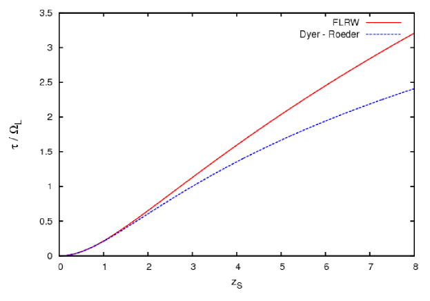
Figure 3.4: Total lensing optical depth $\tau$ in the FLRW (solid line) and Dyer-Roeder (dashed line) formalisms as a function of the redshifts $z$ of sources, assuming point mass lenses.

Figure 3.4 shows the total lensing optical depth assuming point mass lenses. The optical depth is presented as a function of the redshift $z_{S}$ of the sources.

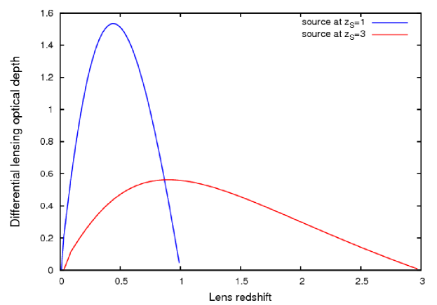
Figure 3.5: Differential lensing optical depth $d\tau/dz$ normalized to 1 in the FRLW formalism as a function of redshifts $z$ of the lens. The blue line indicates the case with a source at redshift 1 and the red line a source at redshift 3. The differential probability has been calculated using a point lens mass model.

3.4.3 Lensing Probability by Singular Isothermal Sphere

The SIS model is described in section 3.3.6. The cross-section for lensing by the SIS is given by equation:

$$\sigma=\pi r^{2}_{eff}=16\pi^{3}\left(\frac{\nu}{c}\right)^{4}\left(\frac{D_{OL}D_{LS}}{D_{OS}}\right)^{2}$$ (3.39)

The differential probability of lensing is:

$$d\tau=n_{0}(1+z_{L})^{3}\sigma\frac{cdt}{dz_{L}}dz_{L}=F(1+z_{L})^{3}\left(\frac{D_{OL}D_{LS}}{R_{0}D_{OS}}\right)^{2}\frac{1}{R_{0}}\frac{cdt}{dz_{L}}dz_{L}\,,$$ (3.40)

where:

$$\frac{cdt}{dz_{L}}=\frac{R_{0}}{1+z_{L}}\frac{1}{\sqrt{\Omega_{\lambda}(1+z_{L})^{3}+(1-\Omega_{\lambda}-\lambda_{0})(1+z_{L})^{2}+\lambda_{0})}}\,,$$ (3.41)

and $F$ is a quantity which measures the effectiveness of matter in producing double images (Turner et al., 1984) and is given by equation:

$$F=16\pi^{3}n_{0}\left(\frac{\nu}{c}\right)^{4}R_{0}^{3}.$$ (3.42)

The value of $F$ used by Fukugita et al. (1992) was 0.047. The total probability of lensing is calculated as in equation (3.38).

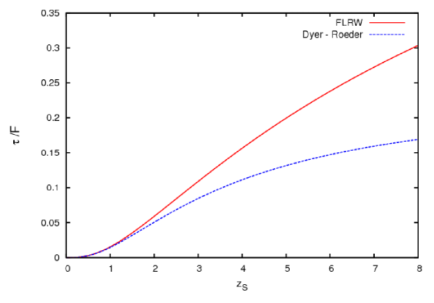
Figure 3.6: Total lensing optical depth $\tau$ in the FRLW (solid line) and Dyer-Roeder (dashed line) formalisms as a function of redshifts $z$ of the source.

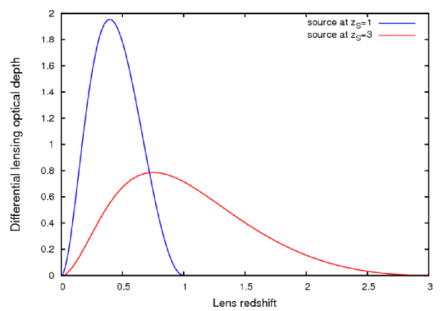
Figure 3.7: Differential lensing optical depth $d\tau/dz$ normalized to 1 in the FRLW formalism as a function of redshift $z$ of the lens. The blue line indicates the case with a source at redshift 1 and the red line a source at redshift 3. The differential probability has been calculated using SIS as a lens model.

Part IV Gravitational lensing in high energy

4.1 Introduction

The precise estimation of the time delay between components of lensed Active Galactic Nuclei (AGN) is crucial for modeling the lensing objects. In turn, more accurate lens models give better constraints on the Hubble constant. Recent years, more than 200 strong lens systems have been discovered, most of them by dedicated surveys such as the Cosmic Lens All-Sky Survey (Myers et al., 2003; Browne et al., 2003) and the Sloan Lens ACS Survey (Bolton et al., 2004).

The launch of the FERMI satellite (Atwood et al., 2009) in 2008 gives the opportunity to investigate gravitational lensing phenomena with high energy gamma rays. The observation strategy of FERMI-LAT, which surveys the whole sky in 190 minutes, allows a regular sampling of quasar light curves with a period of a few hours.

The multiple images of a gravitational lensed AGN cannot be directly observed with high energy gamma-ray instruments such as FERMI-LAT, Swift or ground based Cherenkov telescopes, due to their limited angular resolutions. The angular resolution of these instruments is at best a few arcminutes (in the case of the H.E.S.S.), when the typical separation of the images for quasar lensed by galaxies is a few arcseconds.

The analysis described in this part of my thesis is concerned on the time delay estimation in strong lenses when only spatially unresolved data are available. I have developed a method that handles the problem of poor instrument angular resolution (Barnacka et al., 2011). It is based on the so-called ”double power spectrum” analysis.

The method of time delay estimation have been tested on simulated light curves and on FERMI LAT observations of the very bright radio quasar PKS 1830-211, for which the time delay was previously estimated by Lovell et al. (1998) using radio observations.

This part of the thesis is organized as follows: first, I discus the lensing probability of the FERMI AGNs (section 4.2), then I give a very brief summary of the properties of PKS 1830-211(section 4.3), of the FERMI LAT satellite (section 4.4) and the data towards this AGN (section 4.5). In section 4.6, I discus the methods for time delay estimation. Section 4.7 describes the measurement of the time delay between the two compact components of PKS 1830-211. Section 4.8 contains the summary of results. The last section (4.9), is devoted to gravitational lens time delay and the Hubble constant.

4.2 Probability of lensing of FERMI AGNs

The 2st FERMI catalogue (Nolan et al., 2012) contains 1873 sources detected in the 100 MeV to 100 GeV range. Among the AGN associations the 2st FERMI catalogue lists 1064 blazars, consisting of 432 BL Lacertae objects (BL Lacs), 370 flat-spectrum radio quasars (FSRQs), and 262 of unknown type. From the formalism described in part III the expected numbers of lenses in the FSRQ class is 9.4$\times F$ - assuming the homogeneous FLRW model of the universe, and 8.25$\times F$ for the Dyer-Roeder model.

The probability of lensing was also calculated for BL Lacs objects. The expected number of lenses is 0.61$\times F$ for the FLRW model and 0.58$\times F$ for the Dyer-Roeder model. The AGN are lensed by galaxies which are modeled as SIS lenses (chapter III). The total probability of lensing by SIS lenses is shown on figure 3.6.

The large difference in number of expected lensed objects in FSRQ and BL Lac groups is arising from the redshift distribution of both groups. The BL Lac objects have been detected only at small redshifts below 1.5. Most of them have a z $<$ 0.5. with majority below 0.5. In addition, only half of BL Lac objects have measured redshift. It is very difficult to measured redshift of BL Lac object since this objects are lineless.

The FSRQ have been detected at much larger distances. The most distant FSRQ in FERMI catalog was detected at a redshift $>$ 3. The redshift distribution for BL Lac and FSRQ objects from the second FERMI catalogue is shown on figure 4.1

The lensing probability calculated above does not take into account the magnification bias. The magnification bias can substantially increase the probability of lensing for bright optical quasars (Turner, 1980; Turner et al., 1984; Narayan & Wallington, 1993).

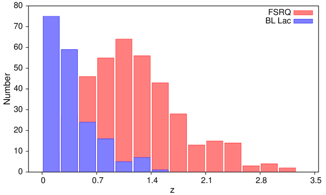
Figure 4.1: The redshift distribution of FSRQ and BL Lac objects included in second Fermi catalogue.

4.3 The PKS 1830-211 gravitational lens system

PKS 1830-211 is one of the object observed in the high energy domain by the FERMI satellite. PKS 1830-211 is a variable, bright radio source and an X-ray blazar. Its redshift was measured to be z=2.507 (Lidman et al., 1999).

The blazar was detected in $\gamma$-rays with EGRET. The association of the EGRET source with the radio source was done by Mattox et al. (1997). The classification of PKS 1830-211 as a gravitational lensed quasi-stellar object was first proposed by Pramesh Rao & Subrahmanyan (1988).

The lensing galaxy is a face-on spiral galaxy, identified by Winn et al. (2002) and Courbin et al. (2002), and located at redshift z=0.89 (Wiklind & Combes, 1996).

PKS 1830-211 is observed in radio as an elliptical ring-like structure connecting two bright sources distant of roughly one arcsecond (Jauncey et al., 1991), see figure 4.5. The compact components were separately observed by the Australia Telescope Compact Array at 8.6 GHz for 18 months. These observations and the subsequent analysis made by Lovell et al. (1998) gave a magnification ratio between the 2 images of $1.52\pm 0.05$ and a time delay of $26^{+4}_{-5}$ days. A separate measurement of a time delay of $24^{+5}_{-4}$ days was made by Wiklind & Combes (2001) using molecular absorption lines.

4.4 The FERMI Satellite

The FERMI Gamma-ray Space Telescope is a space observatory aimed at performing gamma-ray astronomy observations. Fermi was launched on 11 June 2008. The key scientific goals of the FERMI mission are then studies of active galaxy nuclei, supernova remnants, gamma-ray bursts and dark matter.

The observatory includes two scientific instruments. One is a calorimeter, the Large Area Telescope (LAT) sensitive to photons in energy range from 30 MeV to 300 GeV. The LAT field of view is about 20% (2 sr) of the sky. The second instrument is a Gamma-ray Burst Monitor (GBM) used to detect gamma-ray bursts in the energy range from a few keV to 30 MeV.

4.5 FERMI LAT data on PKS 1830-211

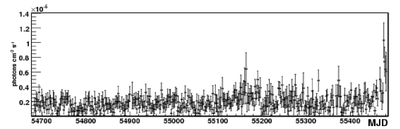
Figure 4.2: Fermi LAT light curve of PKS 1830-211, with a 2 days binning. Photons with energy between 300 MeV and 300 GeV were selected.

PKS 1830-211 has been detected by the FERMI LAT instrument with a detection significance above 41 FERMI Test Statistic (TS), equivalent to a 6 $\sigma$ effect (Abdo et al., 2010b). The long-term light curve is presented on figure 4.2 with a two days binning and the counts map centered at position of PKS 1830-211 (figure 4.3).

The data analysis was performed using a two days binning, which provides a sufficient photon statistic per bin with a time span per bin much shorter than 28 days. The data analysis was cross-checked by binning the light-curve into 1 day and 23 hours bins, with similar results.

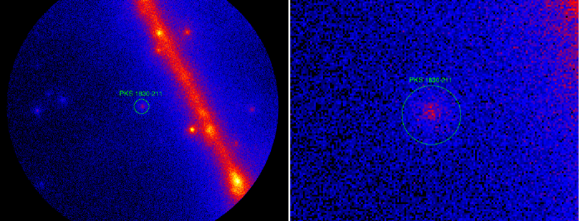
Figure 4.3: Fermi count map centered on PKS 1830-211. Photons in the energy range from 300 MeV to 300 GeV were selected.

The data were taken between August 4 2008 and October 13 2010, and processed by the publicly available Fermi Science Tools version 9. The v9r15p2 software version and the P6_V3_DIFFUSE instrument response functions have been used. The light curve has been produced by aperture photometry, selecting photons from a region with radius 0.5 deg around the nominal position of PKS 1830-211 and energies between 300 MeV and 300 GeV.

4.6 Methods of Time Delay estimation

The most popular methods of time delay estimation, in the context of gravitational lensing, are the cross-correlation method (Kundic et al., 1997), and the dispersion spectra method (Pelt et al., 1996).

In the case of PKS 1830-211, the previous time delay estimation given by Lovell et al. (1998) based on the dispersion analysis method (Pelt et al., 1994, 1996). The light curve analysis has been performed using the data taken from 1997 January to 1998 July. The observation was done with the Australian Telescope Compact Array operating at 8.6 GHz. The light curves taken from Lovell et al. (1998) is shown on figure 4.5.

Figure 4.4: (a) The 8.6 GHz light curve for both components of PKS 1830-211. (b) Light curves superimposed applying the dispersion analysis with a time delay of -23 days and magnification ratio 1.52. Figure is taken from Lovell et al. (1998).

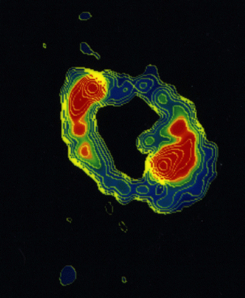
Figure 4.5: High-resolution radio image of PKS1830–211 obtained from the VLBI interferometric radiotelescope networks. The image shows an elliptical ring-like structure connecting the two brighter components separated by distance of one arcsecond. Image credited from Jauncey et al. (1991)

The radio image (figure 4.5) shows two bright, well resolved components connected by an elliptical ring like structure. The analysis presented in Lovell et al. (1998) decomposes the observed system into two lensed images $S_{1}(t)$ and $S_{2}(t)$ and an additional component from the ring like structure. The total observation flux density was thus defined as:

$$S_{m}(t)=S_{1}(t)+S_{2}(t)+S_{ring}\,.$$ (4.1)

The intensity of the lensed images changes in time in similar fashion, but the light curves are shifted in time by $\Delta\tau$. The flux of the two magnifier images change with time but the magnification ratio $\mu$ is constant. Thus, the flux of the second image can be define as:

$$S_{2}(t)=\frac{1}{\mu}S_{1}(t+\Delta\tau)\,.$$ (4.2)

Lovell et al. (1998) followed the analysis of Pelt et al. (1994, 1996). They obtain two light curved datasets $a_{i}$ and $b_{i}$ ($i=1,...,N$ where $N$ is a number of observations) for every data value of $\mu$ and $\Delta\tau$.

The dispersion $D^{2}$ of combined light curves is given by:

$$D^{2}(\Delta\tau,\mu)=\frac{\sum_{ij}W_{ij}V^{{}^{\prime}}_{ij}(a_{i}-b_{j})^{2}}{2\sum_{ij}W_{ij}V^{{}^{\prime}}_{ij}}\,,$$ (4.3)

where $V^{{}^{\prime}}_{ij}$ are weights which select only pairs of observations whose observing time t, do not differ more than $\delta t$.

and $W_{ij}$ is a combined statistical weight defined as

$$W_{ij}=\frac{W_{i}W_{j}}{W_{i}+W_{j}}\,,$$ (4.4)

where $W_{i}=\frac{1}{\sigma^{2}_{i}}$ and $W_{j}=\frac{1}{\sigma^{2}_{j}}$ are the errors from the observations. Equation (4.3) represents the weighted sum of the squared difference between $a_{i}$, $b_{i}$ pairs over the entire light curve. $D^{2}$ is minimized with respect to $\Delta\tau$ and $\mu$. Lovell et al. (1998) obtain a time delay of $26^{+4}_{-5}$ days and a magnification ratio $\mu=1.52\pm 0.05$.

4.7 Double power spectrum method

At the high energy (HE $>$ 100 MeV) domain, the multiple images of a lensed AGN cannot be directly observed due to the limited angular resolution of the existing detectors. This section presents a new method for estimating the time delay of the images of a lensed quasar (Barnacka et al., 2011). This method is usable when the images are unresolved.

4.7.1 Idea

As it was discussed in part III, if a distant source (in our case an AGN) is gravitationally lensed, the light reaches the observer through at least two different paths. For the moment only two light paths are assumed. In reality, the light curves of the two images are not totally identical since (in addition to differences due to photon noise) the source can be microlensed in one of the two paths. The microlensing is cased by a star from the lensing galaxy crossing one of the paths.

Neglecting for the moment the background light and the differences due to microlensing, the observed flux can be decomposed into two components. One of the components is the intrinsic AGN light curve, given by $f(t),$ with Fourier transform $\tilde{f}(\nu).$ The other component has a similar time evolution than the first one, but is shifted in time with a delay $a.$ In addition, the brightness of the second component differs by a factor $b$ from that of the first component, so that it can be written as $bf(t+a)$ and its transform to the Fourier space gives $b\tilde{f}(\nu)e^{-2\pi i\nu a}$.

The sum of two component gives

$$g(t)=f(t)+bf(t+a)\,,$$ (4.5)

which transforms into

$$\tilde{g}(\nu)=\tilde{f}(\nu)(1+be^{-2\pi i\nu a})\,,$$ (4.6)

in Fourier space.

The power spectrum $P_{\nu}$ of the source is obtained by computing the square modulus of $\tilde{g}(\nu)$:

$$P_{\nu}=|\tilde{g}(\nu)|^{2}=|\tilde{f}(\nu)|^{2}(1+b^{2}+2bcos(2\pi\nu a))\,.$$ (4.7)

The measured $P_{\nu}$ is the product of the “true” power spectrum of the source times a periodic component with a period (in the frequency domain) equal to the inverse of the relative time delay $a$. The microlensing of one of the components, when taken into account, gives a modulation of the amplitude of the oscillatory pattern at low frequencies.

The typical time interval for a quasar to cross its own diameter $R_{source}$ is

$$t_{cross}=R_{source}/v_{\perp}\approx 4R_{15}v^{-1}_{600}\,{\rm months}\,,$$ (4.8)

where $R_{15}$ is the quasar size in units of $10^{15}\,$cm, and $v_{\perp}$ is a transverse velocity, perpendicular to the line of sight, here $v_{600}$ in 600 km/s. The typical time of a caustic crossing microlensing event is thus a few months (Wambsganss, 2001). Therefore, only frequencies under $310^{-7}$ Hz will be affected by microlensing event.

The usual way of measuring the time delay $a$ is to calculate the autocorrelation function of f(t). This method was investigated by Geiger & Schneider (1996). The computation of the autocorrelation of a light curve with uneven sampled data is described in Edelson & Krolik (1988).

The Fermi light curve of PKS 1830-211 has very few gaps, and only one notable four-day gap. The missing data have been linearly interpolated. However, simulations with an artificial gap have shown that the results are little affected by this gap. The autocorrelation function can be written as the sum of three terms.

One of these terms models the ”intrinsic” autocorrelation of the AGN, decreasing with a time constant $\lambda$. If $\lambda$ is larger than $a$, the autocorrelation method fails, because the time delay peak merges with the intrinsic component of the AGN. Another potential problem with the autocorrelation method is the sensitivity to spurious periodicities such as the one coming from the motion and rotation of the Fermi satellite.

The periodic modulation of $P_{\nu}$ suggests the use of another method, based on the computation of the power spectrum of $P_{\nu}$, noted $D_{a}$. This method is similar in spirit to the cepstrum analysis (Bogert et al., 1963) used in seismology and speech processing.

If $|\tilde{f}(\nu)|^{2}$ were a constant function of $\nu$, $D_{a}$ would have a peak at the time delay $a$. In the general case, $D_{a}$ is obtained by the convolution of a Dirac function, coming from the cosine modulation, by the Fourier transform of the function:

$$\tilde{h}(\nu)=|\tilde{f}(\nu)|^{2}W(0,\nu_{\mbox{max}})\,,$$ (4.9)

where W(0,$\nu_{\mbox{max}}$) is the window in frequency of $P_{\nu}$ and $\nu_{\mbox{max}}$ is maximum available frequency. The Fourier transform h(a) of $\tilde{h}(\nu)$ defines the width of the time delay peak in the double power spectrum $D_{a}$. For instance if $|\tilde{f}(\nu)|^{2}=e^{-\lambda\nu}$ and $\lambda W>>1,$ then the time delay peak in $D_{a}$ has a Lorentzian shape with a FWHM of ${\lambda}/{\pi}.$ For a typical value of $\lambda=10$ days, one has a FWHM of 3 days.

In the next section we describe the calculation of $P_{\nu}$ and $D_{a}$ and illustrate the procedure with Monte Carlo simulations.

4.7.2 Power spectrum calculation

The Fourier transform is a powerful technique to analyze astronomical data, but it requires a proper preparation of the dataset. To avoid problems arising from the finite length of measurements, sampling and aliasing, we use the procedure for data reduction described by Brault & White (1971) and Press et al. (2007).

First the whole light curve is divided into several segments of equal length. The data have to be evenly spaced and the number of points per segment needs to be equal to a power of 2.

The choice of the segment length is a compromise between the spectral resolution and the size of error bars on points in the final spectrum. The resolution of lines increases with the number of points in the segment, but the error on each point in the spectrum decreases as the number of segments.

As suggested by Brault & White (1971), the segments are overlapped to obtain a larger number of segments with a sufficient number of points. Then the data in each segment are transformed with the following procedure:

1. Data gaps are removed by linear interpolation

2. The mean is subtracted from the series to avoid having a large value in the first bin of the transform

3. The data are oversampled to remove aliasing.

4. The light curve is multiply by the window

5. Zeros are added to the end of the series to reduce power at high frequencies

After the interpolation of missing data, and standard operations (oversampling, zero-padding), the power spectrum is calculated in every segment. Figures 4.6 and 4.6 illustrate with the artificial light curve how step 3 of the data processing procedure removes the aliasing. During the procedure evoluation a lot of different window functions have been tested. Monte Carlo simulations show, that for the first power spectrum calculation, most efficient was a rectangular window function. The rectangular windows function had the smallest smoothing effect on the oscillations expected when the signal is delayed. Finally, the power spectrum is averaged over all segments.

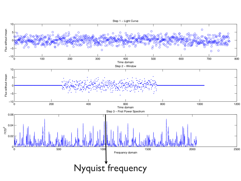
Figure 4.6: Plot illustrating processing of an artificial light curve. Top plot shows an artificial light curve. Middle one shows the artificial light curve multiply by rectangular window and with added zeros to the end and the beginning of dataset. Bottom plot shows the power spectrum of light curve presented on middle plot. The arrow indicates the Nyquist frequency. The power spectrum is strongly aliased (the amplitudes are not going to zero when frequencies are going to Nyquist frequency). Units of x-axises are arbitrary.

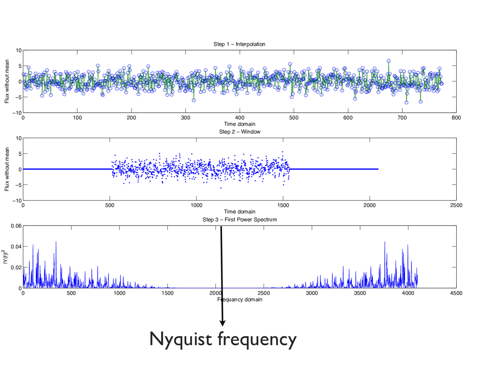
Figure 4.7: Top plot shows the artificial light curve with doubled points. Middle plot shows this artificial light curve multiply by rectangular window and with zeros added to both ends of the series. Bottom plot shows the power spectrum of light curve presented on middle plot. The arrow indicates the Nyquist frequency. After doubling the points the power spectrum is not aliased any more (the amplitude goes to zero when frequency goes to Nyquist frequency). Units of x-axises are arbitrary. Bottom figure presents the power spectrum calculated with just one data slice.

4.7.3 Monte Carlo simulations

Artificial light curves were produced by summing three simulated components. The light curve of PKS 1830-211 shown on figure 4.2 does not exhibit any easily recognizable features, but has a rather random-like aspect. The first component was thus simulated as a white noise, with a Poisson distribution. It would be more realistic to use red noise instead of white noise but the latter is sufficient for most of our purposes, such as computing $D_{a}.$ The second component is obtained from the first by shifting the light curve with a 28 days time lag. The effect of differential magnification of the images has also been included. The background photon noise was taken into account by adding a third component with a Poisson distribution.

The mean number of counts per 2 day bin for PKS 1830-211 is 5.42. This value was used to generate artificial light curves. The first and second components account for 80% of the simulated count rate and the rest is contributed by the Poisson noise.

The power spectrum obtained with an artificial light curve is shown on figure 4.8.

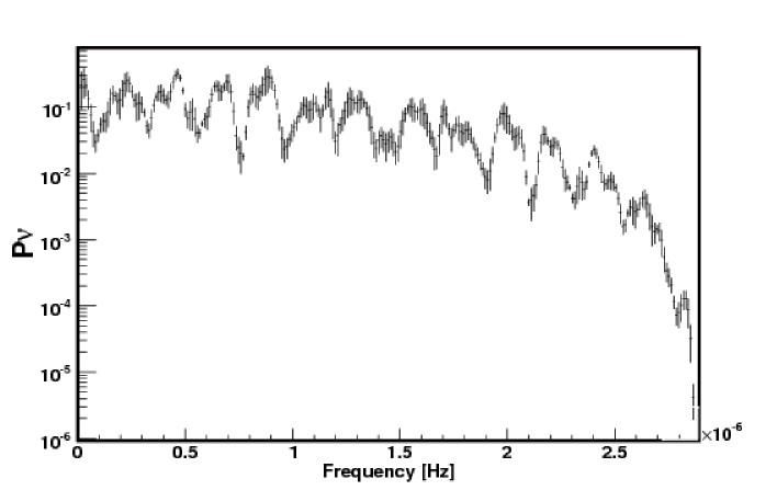
Figure 4.8: Simulated power spectrum of a lensed AGN with a time delay between images of 28 days. The power $P_{\nu}$ is in arbitrary units.

4.7.4 Time delay determination

The methods of time delay determination use the power spectrum $P_{\nu}$ obtained as described in the previous section. The simulated $P_{\nu}$ presented on figure 4.8 shows a very clear periodic pattern. From equation (4.7), it is known that the period of the observed oscillations is equal to the inverse of the time delay between the images.

The preferred approach here was to calculate a so-called double power spectrum $D_{a}$. As in section 4.7.2, the power spectrum $P_{\nu}$ has to be prepared before undergoing a Fourier transform to the “time delay” domain. The low frequency part ($\nu<1/55\mbox{day}^{-1}$) of $P_{\nu}$ was cut off. This cut arises because of the large power observed at low frequencies in the power spectrum of PKS 1830-211.

The high frequency part of the spectrum $P_{\nu}$ was also removed because the power at high frequency is small (it goes to 0 at the Nyquist frequency). The calculation of $D_{a}$ proceeds like in section 4.7.2, except that the $P_{\nu}$ data are bent to zero by multiplication with a cosine bell. This eliminates spurious high frequencies when zeros are added to the $P_{\nu}$ series.

The $D_{a}$ distribution is estimated from 5 segments of the light curve. In every bin of the $D_{a}$ distribution, the estimated double power spectrum is given by the average over the 5 segments. The errors bars on $D_{a}$ are estimated from the dispersion of bin values divided by 2 (since there are 5 segments). Due to the random nature of the sampling process, some of the error bars obtained are much smaller than the typical dispersion in the $D_{a}$ points. To take this into account, a small systematic error bar was added quadratically to all points. The result (with statistical error bars only) is presented on figure 4.9.

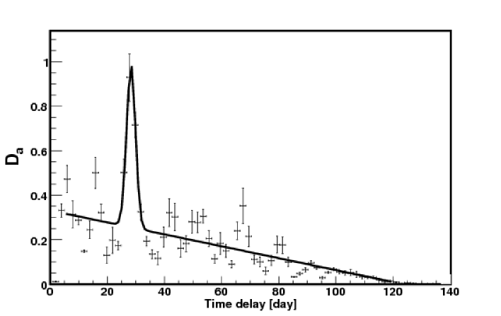
Figure 4.9: Double power spectrum $D_{a}$ for the simulated lensed AGN of figure 4.8. $D_{a}$ is plotted in arbitrary units. The solid line is a fit to a linear plus Gaussian profile.

As described in section 4.7.2, we simulated light curves with a time delay of 28 days. A peak is apparent near a time delay of 28 days on the $D_{a}$ distribution shown on figure 4.9. The points just outside the peak are compatible with a flat distribution. Including also the points in the peak gives a distribution which is incompatible with a flat distribution at the 12.9 sigma level. The parameters of the peak were determined by fitting the sum of a linear function for the background plus a Gaussian function for the signal. In the case shown on figure 4.9, the time delay estimated from $D_{a}$ is $28.35\pm 0.56$ days.

As mentioned in section 4.7.1, the usual approach for the time delay estimation is to compute the autocorrelation of the light curve. The auto-covariance is obtained by taking the real part of the inverse Fourier transform of $P_{\nu}$. The auto-covariance is normalized (divided by the value at zero time lag) to get the autocorrelation. The autocorrelation function of an artificial light curve simulated as in section 4.7.2 is presented on figure 4.10.

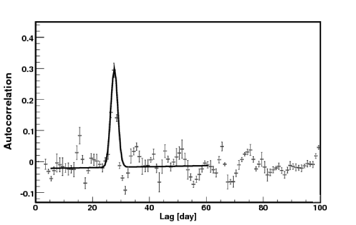
Figure 4.10: Autocorrelation function of the simulated lensed AGN of figure 4.8. The solid line is a fit to a linear plus Gaussian profile.

A peak with a significance of roughly 16 $\sigma$ is present at $27.85\pm 0.14$ days. However the significance of this peak is overestimated since light curves are simulated with white noise instead of red noise. The autocorrelation function of a light curve driven by red noise is given by $e^{-a/\lambda}.$ In the case of our simulated light curves, $\lambda=0$, so that the peak is a little affected by the background of the AGN.

For the simulated light curves, both approaches of time delay determination give reasonable and compatible results.

4.8 Results

The results for real data were obtained with the same procedure as was presented for the simulated light curves. Figure 4.11 shows the power spectrum $P_{\nu}$ calculated from the light curve of PKS 1830-211.

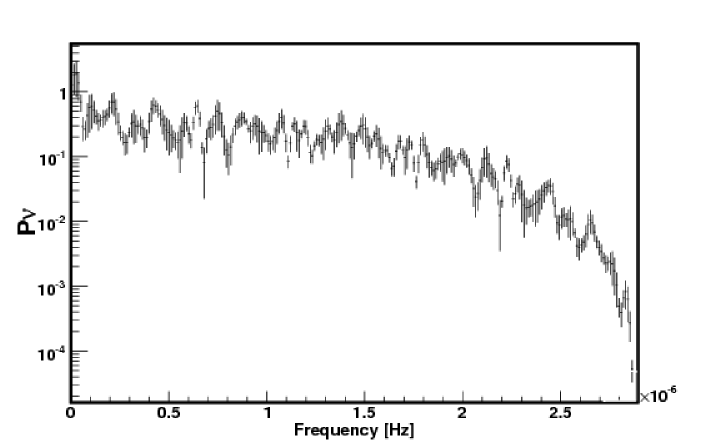
Figure 4.11: Measured power spectrum of PKS 1830-211, plotted in arbitrary units.

An oscillatory pattern is clearly visible in the power spectrum. It is similar to the pattern expected from the simulations shown on figure 4.8.

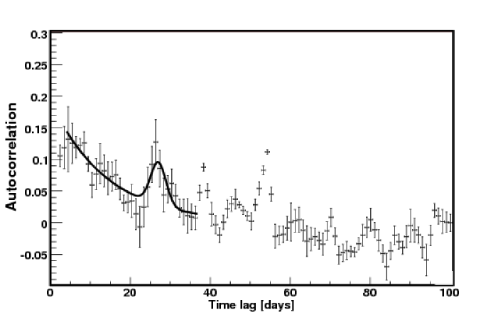
Figure 4.12: Measured autocorrelation function of PKS 1830-211. The solid line is a fit to an exponential plus Gaussian profile.

The autocorrelation function and the $D_{a}$ distribution calculated for real data are shown on figures 4.12 and 4.13.

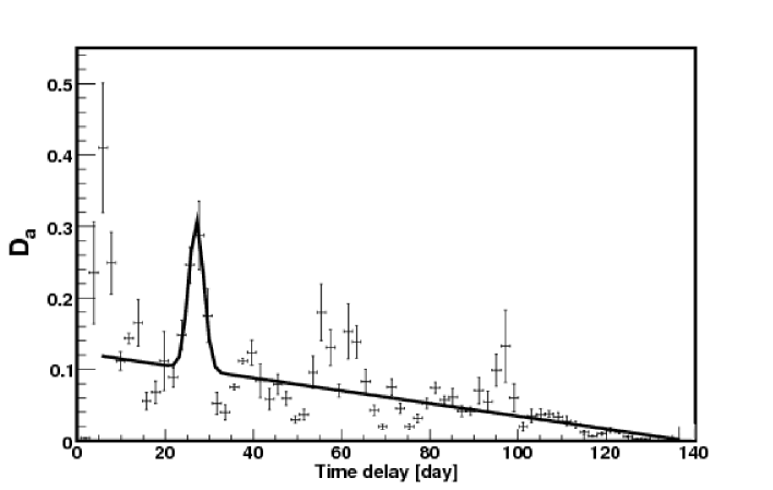
Figure 4.13: Double power spectrum of PKS 1830-211 plotted in arbitrary units. The solid line is a fit to a linear plus Gaussian profile.

A peak around 27 days is seen in both distributions. Several other peaks are present on the autocorrelation function as was already noted by Geiger & Schneider (1996) (see their figure 1).

The peak around 5 days in the $D_{a}$ distribution is likely to be an artefact connected to the time variation of the exposure of the LAT instrument on PKS 1830-211. Using the method described in section 4.7.4, the significance of the peak around 27 days is found to be 1.1 $\sigma$ in the autocorrelation function and 4.2 $\sigma$ in the double power spectrum $D_{a}$. Fitting the position of the peak gives a time delay of $a=27.1\pm 0.6$ days for the $D_{a}$ distribution. The fit of the autocorrelation function to a Gaussian peak over an exponential background gives $a=27.1\pm 0.45$ days. In both cases, the quoted error is derived from the fit.

The double power spectrum distribution obtained for PKS 1830-211 provides the first evidence for gravitational lensing phenomena in high energy gamma rays. The evidence is still at the 4.2 $\sigma$ level but will likely improve by a factor of 2 over the lifetime of the FERMI satellite. Thanks to the uniform light curve sampling provided by FERMI LAT instrument, it is not necessary to identify features on the light curve to apply Fourier transform methods. The example of PKS 1830-211 shows that the method works in spite of the low photon statistic. Possible extensions of the present work are finding multiple delays in complicated lens systems or looking for unknown lensing systems in the FERMI catalog of AGNs.

4.9 Gravitational lens time delay and the Hubble constant

The Hubble constant ($H_{0}$) estimation bases on the distance determination in the Universe. The most common methods of the distances determination in the nearby Universe use the Cepheids, the tip of the red giant branch or maser galaxies. Larger distances are estimated using Tully-Fisher relation for spiral galaxies, the surface brightness fluctuation method or the maximum luminosity of Type Ia supernovae (for full review see Freedman & Madore (2010)). This methods give direct way of $H_{0}$ estimation. However, there are also indirect techniques to estimate $H_{0}$, for example with using the Sunyaev-Zel’dovich effect, the anisotropy in the cosmic microwave effect or the gravitation lensing.

Recently, the most accurate $H_{0}$ estimation is $70.4^{+1.3}_{-1.4}$(km/s)/Mpc. This result was provided with the seven years Wilkinson Microwave Anisotropy Probe (WMAP) observations combined with BAO and $H_{0}$ data (Komatsu et al., 2011). The $H_{0}$ estimated with alternative and independent methods gives consistent value. For example, in the case of gravitational lensing method, the best estimation of $H_{0}$ was obtained with a Bayesian analysis of the strong gravitational lens system B1608+656. This gave $H_{0}=70.6^{+3.1}_{-3.1}\,$(km/s)/Mpc (Suyu et al., 2010).

The $H_{0}$ estimation, based on the lensed quasar PKS 1830-211, has provided rather weak estimation as yet. The value given by Winn et al. (2002) was based on previous time delay measurement and assumption that the lens galaxy has an isothermal mass distribution, they estimate $H_{0}=44\pm 9$ (km/s)/Mpc.

The gravitational lens PKS 1830-211 observed in radio band, consist of two bright components separated by 1 arcsec and connected by ring-like structure. The mass of lensed galaxy can be estimated using the Einstein ring radius $\theta_{E}$ from equation (3.10):

$$M_{L}=\frac{\theta^{2}_{E}c^{2}}{4G}\frac{D_{OL}D_{OS}}{D_{LS}}\,.$$ (4.10)

I will use the $\theta_{E}$ measured from radio ring like structure. The lensed image structure has rather elliptical shape. Therefore, to have more realistic mass estimation in this simplify case, the Einstein radius is measured for two different distances in the elliptical structure (see figure 4.14).

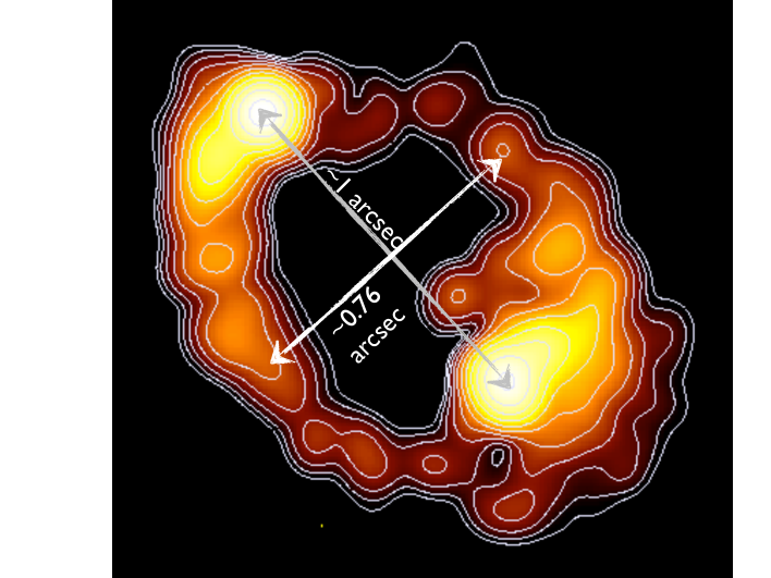
Figure 4.14: The extragalactic gravitational lens PKS 1830-211 with indicated ”Einstein diameters” (Image credit: ATCA).

This approach gives two values of $\theta_{E}$: 0.5 arcsec and 0.38 arcsec. The mass estimated using this values is $6.46\times 10^{10}{\rm h^{-1}M_{\odot}}$ and $3.69\times 10^{10}{\rm h^{-1}M_{\odot}}$, respectively. The distances were calculated using FLRW formalism (see section 3.4.1), $\Omega_{M}=0.3$, $\Omega_{\Lambda}=0.7$ and $H_{0}=100{\rm h(km/s)/Mpc}$. For simplicity, I assumed a point mass lens. Using the time delay between two images separated by 2$\theta_{E}$ given by Lehar (1991) and mass of the lens expressed in units of $h^{-1}$ one can get:

$$h=\frac{1+z_{L}}{\delta t}\frac{4GM}{c^{3}}\left[\frac{\theta_{S}\sqrt{\theta_{S}^{2}+4\theta_{E}^{2}}}{2\theta_{E}^{2}}+\ln{\frac{\theta_{S}+\sqrt{\theta_{S}^{2}+\theta_{E}^{2}}}{|\theta_{S}-\sqrt{\theta_{S}^{2}+\theta_{E}^{2}}|}}\right]\,.$$ (4.11)

where $\theta_{S}$ is the angle between the position of the lensed galaxy and the true (undeflected) position of the background source. Usually, $\theta_{S}$ is obtain from detail lens modeling. In my analysis I used magnification $\mu=1.52\pm 0.05$ ratio provided by Lovell et al. (1998). The magnification factor $\mu_{\pm}$ for a point mass lens is:

$$\mu_{\pm}=\left[1-\left(\frac{\theta_{E}}{\theta_{\pm}}\right)^{4}\right]^{-1}=\frac{u^{2}+2}{2u\sqrt{u^{2}+4}}\pm\frac{1}{2}\,,$$ (4.12)

where $u$ is the angular separation of the source from the point mass lens $\theta_{S}=r_{S}/D_{OL}$ in units of the Einstein angle. The magnification ratio of the two images approximately is:

$$\frac{\mu_{+}}{\mu_{-}}\approx\frac{u+1}{u-1}\,.$$ (4.13)

Using equation (4.13) and the magnification ratio $\mu=1.52\pm 0.05$ one can get $\theta_{S}=0.2\theta_{E}$. The Hubble constant calculated using lens mass and $r_{S}$ obtained above is $H_{0}=61.1\pm 13$ using new time delay and Einstein radius of 0.5 arcsecond, and $H_{0}=35.6\pm 0.5$ for 0.38 arcsec Einstein radius. The most probable value is then $H_{0}=48.7\pm 13.7$.

The strong influence on the accuracy of $H_{0}$ have the systematics errors. Basically, the point mass lens model assumption and value of $\theta_{S}$. The further improvement require reduction of systematics errors by more realistic lens modelling, measurement of the magnification ratio using FERMI data and improvement in the double power spectrum method. The time delay estimation method can be improved when the non-stationary processes like flares or microlensing effect will be taken into account.

Part V Femtolensing of GRBs

5.1 Introduction

Dark matter is one of the most challenging open problems in cosmology or particle physics. A number of candidates for particle dark matter has been proposed over the years (Feng, 2010).

An alternative idea that the missing matter consists of compact astrophysical objects was first proposed in the 1970s (Carr & Hawking, 1974; Hawking, 1974, 1971). An example of such compact objects are primordial black holes (PBHs) created in the very early Universe from matter density perturbations. PBHs would form during the radiation-dominated era, and would be non-baryonic. That satisfy the big bang nucelosynthesis limits on baryons, and PBHs would be thus classified as cold dark matter in agreement with the current paradigm (Cieplak & Griest, 2012). Another famous example is ”brown dwarfs”, excluded by the EROS, MACHO and OGLE searches.

The abundance of PBH above $10^{15}\,$g is a probe of gravitational collapse and large scale structure theory (Carr, 2005). In particular, it constrains the gravitational wave background produced from primordial scalar perturbations in the radiation era of the early Universe (Bugaev & Klimai, 2011).

Recent advances in experimental astrophysics, especially the launch of the FERMI satellite with its unprecedented sensitivity, has revived the interest in PBH physics (Carr et al., 2010; Griest et al., 2011).

In this part, I present the results of a femtolensing search performed on the spectra of GRBs with known redshifts detected by the Gamma-ray Burst Monitor (GBM) on board the FERMI satellite (Barnacka et al., 2012). The non observation of femtolensing on these bursts provides new constraints on the PBHs fraction in the mass range $10^{17}-10^{20}\,$g. I describe in details the optical depth derivation based on simulations applied to each burst individually. The sensitivity of the GBM to the femtolensing detection is also calculated.

This chapter is organized as follows: The first section introduces Primordial Black Holes (PBH). In section  5.3 the basics of femtolensing are given. Section 5.5 describes the data sample and simulations. In section 5.6 the results are presented, while section 5.7 is devoted to discussion and conclusions.

5.2 Primordial Black Holes

As I mentioned in the introduction section, PBHs could have formed in the early Universe. PBHs are not associated with the collapse of a massive star, so that they could have formed with a wide range of masses. In this scenario, the mass of PBH would depend on their formation time $t$:

$$M_{H}(t)\approx\frac{c^{3}t}{G}\approx 10^{15}\left(\frac{t}{10^{-23}\,s}\right)\,\mbox{g}\,.$$ (5.1)

PBH formed at the Planck time ($10^{-43}\,s$) just after the Big Bang would have a mass equal to the Planck mass ($10^{-5}\,$g). However, those formed 1 s after the Big Bang would have a mass of $10^{5}M_{\odot}$.

Bekenstein (1973) and Hawking (1974) discovered that black holes produce a thermal radiation with a temperature:

$$T=\frac{\hbar c^{3}}{8\pi GMk}\approx 10^{-7}\left(\frac{M}{M_{\odot}}\right)^{-1}\,\mbox{K}\,.$$ (5.2)

The radiation has a black body spectrum and is inversely proportional to black hole mass. Black holes of mass M should evaporate on a timescale:

$$\tau(M)\approx\frac{\hbar c^{4}}{G^{2}M^{3}}\approx 10^{64}\left(\frac{M}{M_{\odot}}\right)^{3}\,\mbox{years}\,.$$ (5.3)

Equation (5.3) suggests that PBHs with a mass smaller than $10^{15}\,$g would have evaporated thus far. The $10^{15}\,$g PBHs have a $\sim$ 100 MeV temperature at the present epoch. Observations of the $\gamma$-ray background constrains the density of PBH with masses of less than $10^{15}\,$g. A recent analysis of EGRET data (Lehoucq et al., 2009) shows that the PBH density does not exceed $10^{-8}$ times the critical density.

5.3 Femtolensing

One of the most promising ways to search for PBHs is to look for lensing effects caused by these compact objects. Since the Schwarzschild radius of PBH is comparable to the photon wavelength, the wave nature of electromagnetic radiation has to be taken into account. In such a case, the lensing caused by PBHs introduces an interferometry pattern in the energy spectrum of the lensed object (Mandzhos, 1981). This effect is called ’femtolensing’ (Gould, 1992) due to the $\sim 10^{-15}$ arcseconds angular distance between the images of a source lensed by a $10^{18}\,$g lens. The phenomenon has been a matter of extensive studies in the past (Gould, 2001), but the research was almost entirely theoretical since no case of femtolensing has been detected as yet. Gould (1992) first suggested that the femtolensing of gamma-ray bursts (GRBs) at cosmological distances could be used to search for dark matter objects in the $10^{17}-10^{20}\,$g mass range. Femtolensing could also be a signature of another dark matter candidate: clustered axions (Kolb & Tkachev, 1996).

5.3.1 Magnification and spectral pattern

Consider the lensing of a GRB event by a compact object. The magnification of a point like source has been introduced in section 3.3.3. Equation (3.20) indicates that the magnification depends on the phase. When the two lights paths are not temporally coherent equation (3.20) is reduced to the two first components.

In the case of femtolensing, the phase shift between the two images is:

$$\Delta\phi~{}=~{}\frac{E~{}\delta t}{\hbar},$$ (5.4)

where $E$ is the energy of the photon. The energy dependent magnification produces fringes in the energy spectrum of the lensed object. The magnification pattern for different configurations is presented on figure 5.1 as a function of the photon energy.

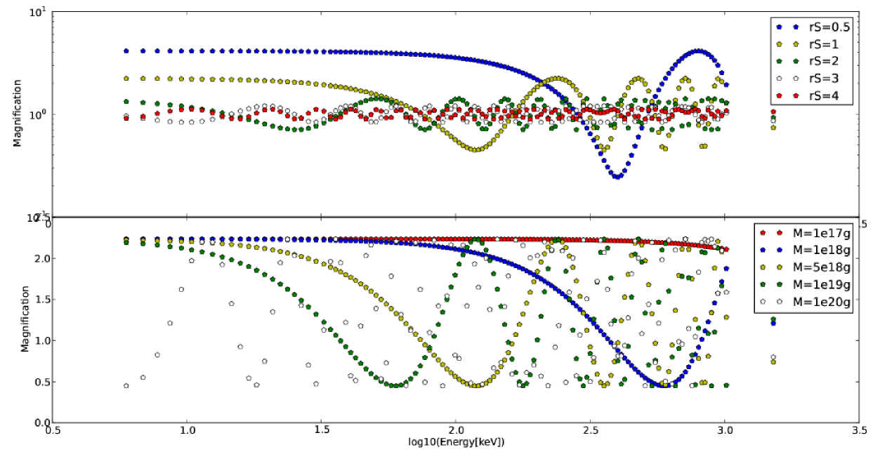
Figure 5.1: Magnification pattern for different lens masses $M$ and projected distances of the source to the lens ($r_{S}$) in the lens plane. The points have been calculated at the values of the energy channels of the GBM detector.

5.3.2 Lensing probability

The lensing probability of gamma ray burst events is calculated in two steps. First, the optical depth $\tau$ for lensing by compact objects is calculated according to the formalism described in section 3.4. The cosmological parameters used in the calculation are: a mean mass density $\Omega_{M}=0.3$ and a normalized cosmological constant $\Omega_{\Lambda}=0.7.$ The calculations are made for both the FLRW and the Dyer & Roeder (1973) cosmology. In the sample, the GRB redshift $z_{s}$ is known. The lens redshift $z_{L}$ is assumed to be given by the maximum of the $d\tau/dz_{L}(z_{S})$ distribution (see figure 3.5). When $\tau\ll 1,$ the lensing probability $p$ is given by $p=\tau\sigma$ where $\sigma$ is the “lensing cross-section” (see Chap. 11 of Schneider et al. (1992)).

In this analysis, the cross-section is defined in the following way. Fringes are searched in the spectra of GRBs. These fringes are detectable only for certain positions $r_{S}$ of the source. The exact criteria for detectability will be given in section 5.5.3. The maximum and minimum position of $r_{S},$ in units of $r_{E}$ are noted $r_{S,min}$ and $r_{S,max}.$ They are found by simulation and depend on the GRB redshift and luminosity. A minimum value of $r_{S}$ occurs because the period of the spectral fringes becomes larger than the GBM energy range at small $r_{S}$.

The femtolensing “cross-section” is simply

$$\sigma=r^{2}_{S,max}-r^{2}_{S,min}\,.$$ (5.5)

The lensing probability does not depend on the individual masses of lenses, but only on the density of compact objects $\Omega_{CO}$. In the optical depth calculation, an increase in the mass of the lenses is compensated by a decrease in the number of scatterers. Therefore, the constraints for a given mass depend only on the cross section $\sigma$.

5.4 FERMI Gamma-ray Bursts Monitor GBM

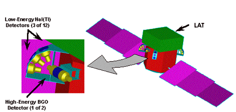
Figure 5.2: The GBM detector on-board of FERMI sattelite. Image credited from http://gammaray.msfc.nasa.gov/gbm/instrument/description/

The Gamma-Ray Burst (GBM) detector (Meegan et al., 2009) on-board the Fermi satellite consists of 12 NaI and 2 BGO scintillators which cover the energy range from 8 keV up to 40 MeV in 128 energy bins. The energy resolution at 100 keV reaches $\sim$15% and $\sim$10% at 1 MeV. These detectors monitor the entire sky. The GBM can locate a burst with an accuracy of $<$ 15 deg. Currently, the average burst trigger rate is $\sim$ 260 bursts per year. In the first two years of operation, the GBM triggered on roughly 500 GRBs.

5.5 Data analysis

In our analysis, we use a sample of GRBs with known redshifts. The selection of these bursts is described in section 5.5.1. Each burst is then fitted to a standard spectral model, as explained in section 5.5.2. Finally, the sensitivity of each burst to femtolensing is studied with simulated data. The simulation is described in section 5.5.3.

5.5.1 Data selection

In this analysis, only the bursts with known redshifts have been investigated. The initial sample consisted of 32 bursts taken from Gruber et al. (2011) and 5 additional bursts from the GRB Coordinates Network (GCN) circulars. For 17 bursts, the amount of available data was not sufficient to obtain good quality spectra. The final sample thus consists of 20 bursts, which are listed in table 5.5.

5.5.2 Data processing and spectral analysis

The GBM data are publicly available in the CSPEC format and were downloaded from the FERMI FSSC website . The CSPEC files contain the counts in 128 energy channels with 1.024 s bins for all detectors. Only detectors with a minimal signal to noise ratio of 5.5 in each bin were selected for the analysis. Data were analyzed with the RMfit version 33pr7 program. The RMfit software package was originally developed for the time-resolved analysis of BATSE GRB data but has been adapted to GBM and other instruments. The observed data is a convolution of the GRB photon spectrum with an instrument response function. This is illustrated on figure 5.3. For each detector with sufficient data, the background was subtracted and the counts spectrum of the first ten seconds of the burst (or less if the burst was shorter) was extracted.

The energy spectrum was obtained with a standard forward-folding algorithm. Several GRB spectral models such as a broken power law (BKN), Band’s model (BAND) or a smoothly broken power law (SBKN) where considered. The femtolensing effect was added as a separate model. The magnification and the oscillating fringes were calculated according to equation (3.20), then multiplied with the BKN or BAND functions.

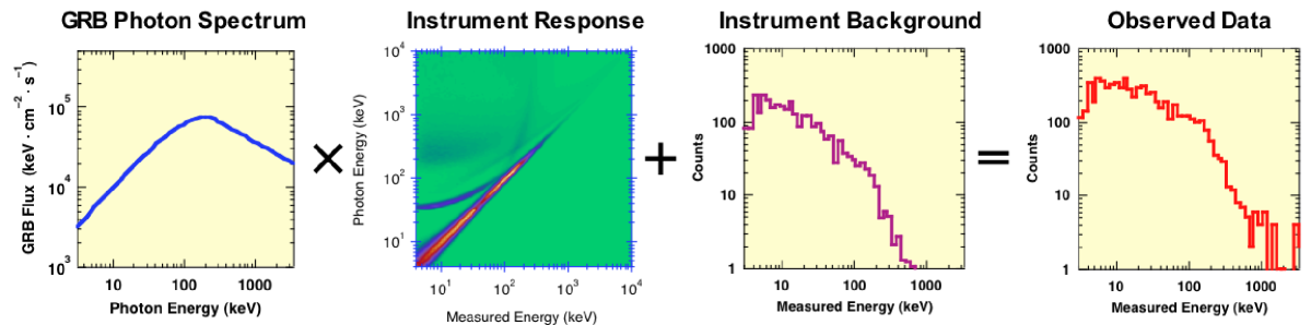
Figure 5.3: Decomposition of observed GBM data. Figure credited from R.M. Kippen (LANL).

5.5.3 Simulations

The detectability of spectral fringes has been studied with simulated signals. The detectability first depends on the luminosity and redshift of the bursts, and second on the detector’s energy resolution and data quality. The sensitivity of the GBM to the lens mass $M$ depends strongly also on the energy range and resolution of the GBM detectors. When small masses are considered, the pattern of spectral fringes appears outside of the energy range. The large masses produce fringes with hardly detectable amplitudes and periods smaller than the energy bin size.

Because the data quality and the background are not easily simulated, the detectability estimation is performed on real data. Namely, GRB events with known redshifts are selected. Since the source redshift is known, the lens redshift is assumed to be the maximum value of $d\tau/dz_{L}(z_{S})$ as explained in section 3.4.2. For a given observed GRB, the femtolensing signal depends thus only on 2 parameters: the lens mass $M$ and the source position in the lens plane $r_{S}.$ The data are then processed as follows:

1. The magnification (equation 3.20) as a function of the energy is calculated for the given lens mass $M$ and position of the source $r_{S}.$

2. This magnification is then convolved with the instrumental resolution matrix to obtain magnification factors for each channel of the detector.

3. The spectral signal is extracted from the data by subtracting the background. It is then multiplied by the corrected magnification.

4. The background is added back.

I now illustrate the detectability calculation with the luminous burst GRB090424592. The spectral data of this burst were first fitted with standard spectral models: BKN, SBKN and BAND. The GRB090424952 burst is best fitted with the BAND model. The BAND model has 4 free parameters: the amplitude A, the low energy spectral index $\alpha$, the high energy spectral index $\beta$ and the peak energy $E_{peak}$ (Goldstein et al., 2012). The fit has $\chi^{2}=78$ for 67 degrees of freedom (d.o.f).

The data are then modified by incorporating the spectral fringe patterns for a range of lens masses $M$ and source positions $r_{S}.$ The simulated data and the corresponding femtolensing fit are presented in figure 5.4.

Figure 5.4: Simulated spectrum obtained with GRB 090424592. The spectrum was fitted with femtolensing$+$BAND model. The fit has $\chi^{2}$ = 79 for 73 d.o.f. The fit parameters are: $A=0.32\pm 0.01\,$ph s${}^{-1}\,$cm${}^{-2}\,$keV^-1, $E_{peak}=179\pm 3\,$keV, $\alpha=-0.87\pm 0.02$ and $\beta=-3.9\pm 7.5$. The simulated femtolensing effect is caused by a lens at redshift $z_{L}=0.256$ acting on a source at $z_{S}=0.544$. The simulated mass is $M=1\times 10^{18}\,$ g and the mass reconstructed from the fit is $1.01\times 10^{18}\,$g. The source is simulated at position $r_{S}=2$. The position reconstructed from the fit is $r_{S}=1.9$.

Figure 5.5: Simulated femtolensed spectrum fitted with the BAND model. The fit has $\chi^{2}=752$ for $75$ d.o.f. The fit parameters are: $A=0.36\pm 0.01\,$ph s${}^{-1}\,$cm${}^{-2}\,$keV^-1, $E_{peak}=174\pm 5\,$keV, $\alpha=-0.8\pm 0.02$ and $\beta=-2.4\pm 0.1$. The SBKN model fit is almost indistinguishable from the BKN model fit.

Neither BKN nor BAND models are able to fit the simulated data (see figure 5.5). The values of $r_{S}$ are then changed until the $\chi^{2}$ of the fit obtained is not significantly different from the $\chi^{2}$ of the unmodified data. More precisely, the $\chi^{2}$ difference $\Delta\chi^{2}$ should be distributed in the large sample limit as a $\chi^{2}$ distribution with 2 degrees of freedom according to Wilk’s theorem (Mattox et al., 1996). The value $\Delta\chi^{2}=5.99,$ which corresponds to a $\chi^{2}$ probability of 5% for 2 d.o.f, was taken as the cut value. The effect of changing $r_{S}$ on the femtolensing model is illustrated on figures 5.6 and 5.7.

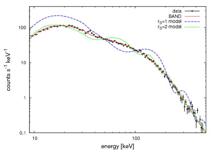
Figure 5.6: The spectrum of GRB 090424592 using NaI detector n7, with the BAND and femtolensing fits superimposed. The parameters are $r_{S}=1$, $2$, and lens mass $1\times 10^{18}\,$g. The models are convolved with the response matrix.

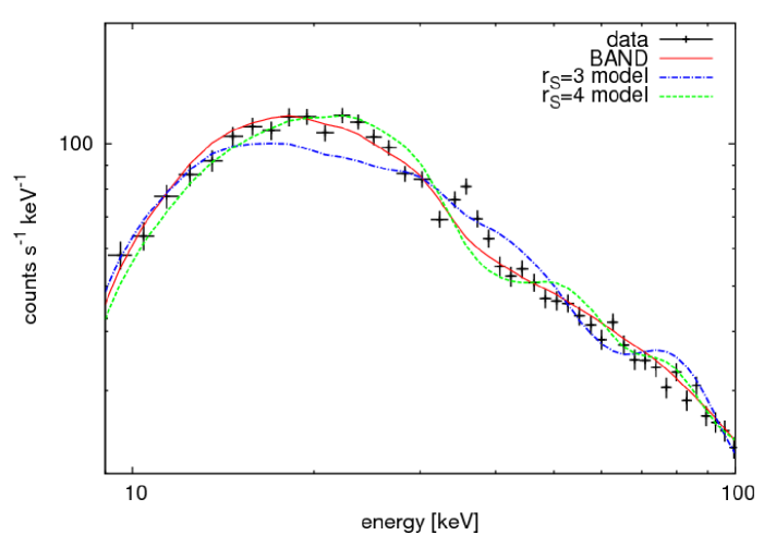
Figure 5.7: The spectrum of GRB 090424592 using NaI detector n7. The BAND and femtolensing fits are superimposed. The parameters are $r_{S}=3$, $4$, and lens mass $1\times 10^{18}\,$g. The excess at $33\,$keV (K-edge) is an instrumental effect seen on many bright bursts.

The pattern in energy is visible when the phase shift between the two images $\Delta\phi~{}\sim~{}\left(E/1MeV\right)\left(M/1.5\times 10^{17}\,g\right)$ is close to 1.

The GBM detector can detect photons with energy from few keV to $\sim$ MeV. Lens masses from $10^{17}\,$g to $10^{20}\,$g are thus detectable with GBM. The femtolensing pattern can be detected when the period of the fringes is larger than the detector energy resolution and smaller than the detector energy range. The value of $r_{S,max}$ comes from the comparison of the period of the oscillating pattern to the detector energy resolution. The value of $r_{S,min}$ arises from the comparison of the period of the fringes to the detector energy range. Because of these constraints, the most sensitive mass range is $10^{18}\,$g to $10^{19}\,$g.

Figure 5.8: Energy of photons affected by femtolensing as a function of the compact lens mass. The dotted arrows indicate the GBM energy range and the solid arrows show the masses which can be best detected by GBM.

In figure 5.9 I show the maximum and minimum detectable $r_{S}$ for different lens masses. The maximum difference between $r_{S,max}$ and $r_{S,min}$ is at $M=1\times 10^{18}\,$g. The largest femtolensing cross-section occurs for this mass.

5.6 Results

The 20 burst sample from table 5.5 have been fitted with the standard BKN, BAND and SBKN models. The models with the best $\chi^{2}$ probability were selected and are shown on table 5.5. The bursts are well fitted by these standard models, so there is no evidence for femtolensing in the data.

As explained in section 5.3.2, the lensing probability for each burst depends on the lens mass and on the $r_{S,min}$ and $r_{S,max}$ values. Since the sensitivity of GBM to femtolensing is maximal for lens masses of $\sim 1\times 10^{18}\,$ g (see figure 5.9), the values of $r_{S,min}$ and $r_{S,max}$ for each event were first determined at a mass $M=1\times 10^{18}\,$ g by simulation. As explained in section 5.3.2, the value of $r_{S,min}$ is set by the period of the spectral fringes so that it is independent of the burst luminosity. The values of $r_{S,max}$ obtained are listed in table 5.5. The lensing probability is then calculated for both the FRLW and Dyer & Roeder cosmological models using the redshift of each burst, the most probable lens position and the values of $r_{S,min}$ and $r_{S,max}$ for the mass $M=1\times 10^{18}\,$g. The number of expected lensed bursts in the sample is the sum of the lensing probabilities. It depends linearly on $\Omega_{CO}.$

Since no femtolensing is observed, the number of expected events should be less than 3 at 95% confidence level (C.L.). The constraints on the density of compact objects $\Omega_{CO}$ is derived to be less than 4% at 95% C.L for both cosmological models. The values of the lensing probabilities for all the bursts in our sample assuming the constrained density of compact objects are shown in table 5.5. The limits at other lens masses are obtained by normalizing the $\Omega_{CO}$ at $M=1\times 10^{18}\mbox{g}$ by the cross section $\sigma$. The cross section is calculated using equation. (5.5) and the values of $r_{S,min}$ and $r_{S,max}$ from figure 5.9. The limits on $\Omega_{CO}$ at $95\%\,$C.L. are plotted in figure 5.10.

Figure 5.9: Minimum and maximum detectable $r_{S}/r_{E}$ as a function of lens mass for GRB 090424592.

Figure 5.10: Constraints on the fraction (or normalized density) of compact objects. The zones above the curves are excluded at the 95% confidence level.

Table 5.5: The sample of 20 GBM GRBs used in the analysis.

				Fit to simulated data
Name	$z_{S}$	Fit to the data		Model	Femtolensing	$r_{S,max}$	$z_{L}$	Lensing Probability
		Model	$\chi^{2}$/d.o.f	$\chi^{2}$/d.o.f	$\chi^{2}$/d.o.f			FRLW	Dyer-Roeder
GBM 080804972	2.2045	BAND	68/74	129/74	80/72	2.5	0.770	0.145	0.145
GBM 080916009C	4.3500	BKN	75/74	115/74	93/72	3	1.087	0.489	0.444
GBM 080916406A	0.6890	BKN	58/57	91/55	67/53	3	0.324	0.031	0.033
GBM 081121858	2.5120	BKN	39/49	63/52	50/50	3	0.829	0.250	0.245
GRB 081222204	2.7000	BKN	73/66	89/62	68/60	3.5	0.859	0.374	0.364
GRB 090102122	1.5470	BAND	81/85	124/85	92/83	3	0.603	0.134	0.127
GRB 090323002	3.5700	BAND	77/77	106/64	95/62	2	0.964	0.173	0.162
GRB 090328401	0.7360	BKN	105/70	124/70	64/68	2.5	0.346	0.024	0.026
GRB 090424592	0.5440	BAND	78/67	215/78	104/76	4	0.256	0.035	0.038
GRB 090510016	0.9030	BKN	62/66	108/98	94/96	1.5	0.406	0.012	0.013
GRB 090618353	0.5400	BAND	59/72	158/69	93/67	3	0.254	0.019	0.021
GRB 090926181	2.1062	BAND	87/81	247/81	123/79	4	0.737	0.348	0.349
GRB 091003191	0.8969	BKN	93/94	140/94	96/92	3	0.400	0.049	0.053
GRB 091020900	1.7100	BKN	74/69	100/69	77/67	3	0.667	0.144	0.147
GRB 091127976	0.4900	BAND	78/74	84/74	71/72	4	0.240	0.029	0.031
GRB 091208410	1.0630	BAND	55/55	101/55	54/53	3	0.457	0.066	0.070
GRB 100414097	1.3680	BKN	65/61	120/68	92/66	2.5	0.560	0.070	0.073
GRB 100814160A	1.4400	BKN	86/70	181/70	110/68	2	0.590	0.049	0.051
GRB 100816009	0.8049	BKN	67/56	83/56	68/54	3	0.360	0.041	0.043
GRB 110731465	2.8300	SBKN	72/64	96/53	78/51	3	0.877	0.292	0.283

5.7 Discussion and conclusions

Cosmological constraints on the PBH abundance are reviewed by Carr et al. (2010). One way to obtain the abundance of PBH is to constrain the density of compact objects $\Omega_{CO}$. Note that the limits on the compact object abundance in the $10^{26}-10^{34}\,$g range obtained with microlensing are at the 1$\%$ level (MACHO in figure 5.11).

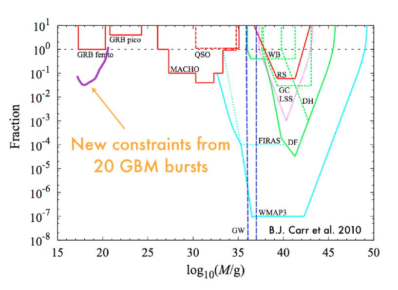
Figure 5.11: Constraints on the fraction of compact objects for the various effects. Figure credited from Carr et al. (2010)

It is stated in Abramowicz et al. (2009) that the mass range $10^{16}\,$g $<M_{BH}<10^{26}\,$g is virtually unconstrained. Indeed, constraints in this mass range were given by just one group (Marani et al. (1999)). The limits are shown on figure 5.11 as GRB femto and pico. Their results is based on a sample of 117 bright bursts detected by the BATSE satellite. The bursts were searched for spectral features by Briggs et al. (1998). The constraints reported by Marani et al. (1999) are $\Omega_{CO}<0.2$ if the average distance to the GRBs is $z_{GRB}\sim 1$ or $\Omega_{CO}<0.1$ if $z_{GRB}\sim 2$.

Under the mass $5\times 10^{14}\,$g, $\Omega_{CO}$ is constrained by PBH evaporation. Above the femtolensing range, the constraints come from microlensing. The new idea by Griest et al. (2011) shows that the microlensing limit could be improved and get constraints down to $10^{20}\,$g with the Kepler satellite observations.

The FERMI satellite was launched three and a half years ago. Since then, almost 1000 of GRB were observed with the GBM detector. In many cases data quality is good enough to reconstruct time-resolved spectra. This unique feature is exploited in our femtolensing search by selecting the first few seconds of a burst in data analysis.

Limits from the present thesis were obtained by selecting only those bursts with known redshifts in the GBM data. This reduces the data sample from the 500 bursts detected in the first 2 years to only 20. The constraints on $\Omega_{CO}$ obtained at the $95\%\,$ C.L. are shown on figure. 5.10. These constraints improve the existing constraints by a factor of 4 in the mass range $1\times 10^{17}$ – $10^{20}\,$g.

After ten years of operation, the GBM detector should collect over 2500 bursts. Only a few of the bursts, say 100, will have a measured redshift and sufficient spectral coverage. By applying the methods described in this thesis, the limits will improve by a factor of 5 reaching a sensitivity to density of compact objects down to the 1% level.

Part VI Conclusions

In this thesis I have presented my work on the Level 2 trigger system for the H.E.S.S. II telescope developed in cooperation with IRFU CEA-Saclay in France. The H.E.S.S. II telescope was built to enlarge the current energy range of the existing H.E.S.S. system down to tens of GeV. In the low energy part of the energy range, the H.E.S.S. II telescope has to carry the observations without the support of the smaller telescopes - in the, so called, monomode. In the monomode, very high trigger rates are expected due to a large flux of single muons. To reduce the trigger rate, the Level 2 trigger system has been implemented in the H.E.S.S. II telescope. The system consists of both hardware and software solutions. My work on the project focused on the algorithm development and the Monte Carlo simulations of the trigger system and overall instrument. I have developed and successfully tested the algorithm suitable to reject a major fraction of the background events and to reduce the trigger rate to the level possible to process by the data acquisition system (Moudden, Barnacka, Glicenstein et al., 2011a, b).

I have also been analyzing the H.E.S.S. data of the particular blazar PKS 1510-089. The work on this blazar concerned the data analysis and modeling of broad-band emission of PKS 1510-089 observed in a flaring state in very high energy (VHE) range by the H.E.S.S. observatory. PKS 1510-089 is an example of the, so-called, flat spectrum radio quasars (FSRQs) for which no VHE emission is expected due to the Klein-Nishina effects and strong absorption in the broad line region (Moderski et al., 2005). Recent detection of at least three FSRQs by Cherenkov telescopes has forced a revision of our understanding of these objects. In this thesis I have presented the analysis of the H.E.S.S. data: a light curve and a spectrum of the PKS 1510-089, together with the FERMI data and a collection of multi-wavelength data obtained by various instruments. I have successfully modeled PKS 1510-089 by applying the single zone internal shock scenario. In this scenario, the highest energy emission is the result of the Comptonization of the infrared photons from the dusty torus (thus avoiding Klein-Nishina limit), while the bulk of the emission in the MeV-GeV range is still dominated by the Comptonization of the radiation coming from the broad line region.

The strategy of observation of FERMI-LAT, which surveys the whole sky in 190 minutes, allows a regular sampling of quasar light curves with a period of a few hours. This gives the opportunity to investigate lensing phenomena with high energy (HE) gamma-rays. However, the multiple images of a gravitational lensed AGN cannot be directly observed with HE gamma-ray instruments due to their limited angular resolutions. I have developed a method of time delay estimation that handles the problem of the limited instrument angular resolution (Barnacka et al., 2011). It is called a ”double power spectrum” analysis and relies on the double Fourier transform of the observed light curves. The method has been tested on simulated light curves and on FERMI LAT observations of the very bright radio quasar PKS 1830-211, for which the time delay of $26^{+4}_{-5}$ days was previously estimated by Lovell et al. (1998) using radio observations. The double power spectrum analysis has resulted in an estimation of the delay of 27.1$\pm$0.6 days, with a statistical uncertainty an order of magnitude better as compared to previous derivations. PKS 1830-211 has thus become the first gravitationally lensed object with its echo detected using the HE instrument.

Dark matter is one of the most challenging open problems in cosmology and particle physics. Although currently the weakly interacting massive particles (WIMPs) seems to be favored as a possible constituent of the dark matter, the alternative idea that the missing matter consists of compact astrophysical objects was also proposed as early as in the 1970s (Carr & Hawking, 1974; Hawking, 1974, 1971). An example of such compact objects might be primordial black holes (PBHs) created in the very early Universe from matter density perturbations. To derive the constraints on the compact object abundance I have search for femtolensing effects in the spectra of gamma-ray bursts with known redshifts detected by the Gamma-ray Burst Monitor (GBM) on board the FERMI satellite. The search involved the analysis of the FERMI data, which have been used to estimate the femtolensing effect detectability. The lack of detection of the femtolensing effect has provided new constraints on the PBHs fraction in the mass range $10^{17}-10^{20}\,$g. Less than 3% of critical density are contributed by PBHs (or any compact objects) at 95% confidence level (Barnacka et al., 2012).

References

- (1)
- (2)
- (3)
- (4)
- (5)
- (6)
- (7)
- (8)
- (9)
- (10)
- (11)
- (12)
- (13)
- (14)
- (15)
- (16)
- (17)
- (18)
- (19)
- (20)
- (21)
- (22)
- (23)
- (24)
- (25)
- (26)
- (27)
- (28)
- (29)
- (30)
- (31)
- (32)
- (33)
- (34)
- (35)
- (36)
- (37)
- (38)
- (39)
- (40)
- (41)
- (42)
- (43)
- (44)
- (45)
- (46)
- (47)
- (48)
- (49)
- (50)
- (51)
- (52)
- (53)
- (54)
- (55)
- (56)
- (57)
- (58)
- (59)
- (60)
- (61)
- (62)
- (63)
- (64)
- (65)
- (66)
- (67)
- (68)
- (69)
- (70)
- (71)
- (72)
- Abdo et al. (2010a) A. A. Abdo, M. Ackermann, I. Agudo et al. Fermi Large Area Telescope and Multi-wavelength Observations of the Flaring Activity of PKS 1510-089 between 2008 September and 2009 June. ApJ, 721 (2010a), 1425–1447
- Abdo et al. (2009) A. A. Abdo, M. Ackermann, M. Ajello et al. Early Fermi Gamma-ray Space Telescope Observations of the Quasar 3C 454.3. ApJ, 699 (2009), 817–823
- Abdo et al. (2010b) A. A. Abdo, M. Ackermann, M. Ajello et al. Fermi-LAT first source catalog (1FGL) (Abdo+, 2010). VizieR Online Data Catalog, 218 (2010b), 80405–+
- Abdo et al. (2010c) A. A. Abdo, M. Ackermann, M. Ajello et al. The First Catalog of Active Galactic Nuclei Detected by the Fermi Large Area Telescope. ApJ, 715 (2010c), 429–457
- Abdo et al. (2011) A. A. Abdo, M. Ackermann, M. Ajello et al. Fermi Gamma-ray Space Telescope Observations of the Gamma-ray Outburst from 3C454.3 in November 2010. ApJ, 733 (2011), L26
- Abramowicz et al. (2009) M. A. Abramowicz, J. K. Becker, P. L. Biermann et al. No Observational Constraints from Hypothetical Collisions of Hypothetical Dark Halo Primordial Black Holes with Galactic Objects. ApJ, 705 (2009), 659–669
- Abramowski et al. (2012) A. Abramowski, F. Acero, F. Aharonian et al. Measurement of the extragalactic background light imprint on the spectra of the brightest blazars observed with H.E.S.S. ArXiv e-prints, (2012)
- Aharonian et al. (2005) F. Aharonian, A. G. Akhperjanian, K.-M. Aye et al. H.E.S.S. observations of PKS 2155-304. A&A, 430 (2005), 865–875
- Aharonian et al. (2006) F. Aharonian, A. G. Akhperjanian, A. R. Bazer-Bachi et al. Observations of the Crab nebula with HESS. A&A, 457 (2006), 899–915
- Aleksić et al. (2011a) J. Aleksić, L. A. Antonelli, P. Antoranz et al. MAGIC Discovery of Very High Energy Emission from the FSRQ PKS 1222+21. ApJ, 730 (2011a), L8
- Aleksić et al. (2011b) J. Aleksić, L. A. Antonelli, P. Antoranz et al. MAGIC Observations and multiwavelength properties of the quasar 3C 279 in 2007 and 2009. A&A, 530 (2011b), A4
- Antonucci (1993) R. Antonucci. Unified models for active galactic nuclei and quasars. ARA&A, 31 (1993), 473–521
- Atwood et al. (2009) W. B. Atwood, A. A. Abdo, M. Ackermann et al. The Large Area Telescope on the Fermi Gamma-Ray Space Telescope Mission. ApJ, 697 (2009), 1071–1102
- Barnacka et al. (2012) A. Barnacka, J.-F. Glicenstein & R. Moderski. New constraints on primordial black holes abundance from femtolensing of gamma-ray bursts. Phs.Rev.D, 86 (2012) 4, 043001
- Barnacka et al. (2011) A. Barnacka, J.-F. Glicenstein & Y. Moudden. First evidence of a gravitational lensing-induced echo in gamma rays with Fermi LAT. A&A, 528 (2011), L3
- Barnacka & Moderski (2009) A. Barnacka & R. Moderski. INTEGRAL OBSERVATION OF GAMMA-RAY QUASAR PKS B1510-089. J. Dumarchez & J. Tran Thanh Van, Very High Energy Phenomena in the Universe, 1 (2009) 111
- Bastieri et al. (2001) D. Bastieri, M. Bettini, C. Bigongiari et al. A two-level pattern trigger for the MAGIC telescope. Nuclear Instruments and Methods in Physics Research A, 461 (2001), 521–523
- Bekenstein (1973) J. D. Bekenstein. Black Holes and Entropy. Phs.Rev.D, 7 (1973), 2333–2346
- Bernlöhr et al. (2003) K. Bernlöhr, O. Carrol, R. Cornils et al. The optical system of the H.E.S.S. imaging atmospheric Cherenkov telescopes. Part I: layout and components of the system. Astroparticle Physics, 20 (2003), 111–128
- Bi & Yuan (2008) X.-J. Bi & Q. Yuan. Cosmology from very high energy $gamma$-rays. ArXiv e-prints, (2008)
- Blackman (1996) E. G. Blackman. Reconnecting Magnetic Flux Tubes as a Source of In Situ Acceleration in Extragalactic Radio Sources. ApJ, 456 (1996), L87
- Blandford (1983) R. D. Blandford. Magnetic fields in astrophysics /Helen B. Warner Prize Lecture/. AJ, 88 (1983), 245–252
- Blandford & Levinson (1995) R. D. Blandford & A. Levinson. Pair cascades in extragalactic jets. 1: Gamma rays. ApJ, 441 (1995), 79–95
- Blandford & Narayan (1992) R. D. Blandford & R. Narayan. Cosmological applications of gravitational lensing. ARA&A, 30 (1992), 311–358
- Blandford & Rees (1978) R. D. Blandford & M. J. Rees. Some comments on radiation mechanisms in Lacertids. A. M. Wolfe, BL Lac Objects (1978) 328–341
- Blandford & Znajek (1977) R. D. Blandford & R. L. Znajek. Electromagnetic extraction of energy from Kerr black holes. MNRAS, 179 (1977), 433–456
- Błażejowski et al. (2000) M. Błażejowski, M. Sikora, R. Moderski et al. Comptonization of Infrared Radiation from Hot Dust by Relativistic Jets in Quasars. ApJ, 545 (2000), 107–116
- Boettcher (2010) M. Boettcher. Models for the Spectral Energy Distributions and Variability of Blazars. ArXiv e-prints, (2010)
- Bogert et al. (1963) B. P. Bogert, M. J. R. Healy & J. W. Tukey. M.Rosenblat, Proceedings on the Symposium on Time Series Analysis, Wiley, NY (1963) 209–243
- Bolton et al. (2004) A. S. Bolton, S. Burles, D. J. Schlegel et al. Sloan Digital Sky Survey Spectroscopic Lens Search. I. Discovery of Intermediate-Redshift Star-forming Galaxies behind Foreground Luminous Red Galaxies. AJ, 127 (2004), 1860–1882
- Bolton et al. (2006) A. S. Bolton, S. Rappaport & S. Burles. Constraint on the post-Newtonian parameter on galactic size scales. Phs.Rev.D, 74 (2006) 6, 061501
- Brault & White (1971) J. W. Brault & O. R. White. The Analysis and Restoration of Astronomical Data via the Fast Fourier Transform. A&A, 13 (1971), 169–+
- Briggs et al. (1998) M. S. Briggs, D. L. Band, R. D. Preece et al. BATSE evidence for GRB spectral features. C. A. Meegan, R. D. Preece, & T. M. Koshut, Gamma-Ray Bursts, 4th Hunstville Symposium, American Institute of Physics Conference Series, 428 (1998) 299–303
- Browne et al. (2003) I. W. Browne, P. N. Wilkinson, N. J. Jackson et al. The Cosmic Lens All-Sky Survey - II. Gravitational lens candidate selection and follow-up. MNRAS, 341 (2003), 13–32
- Bugaev & Klimai (2011) E. Bugaev & P. Klimai. Constraints on the induced gravitational wave background from primordial black holes. Phys. Rev. D, 83 (2011), 083521
- Capdevielee et al. (1993) J. N. Capdevielee, P. Gabriel, H. J. Gils et al. Extensive air shower simulations with the CORSIKA program. L. Jones, Very High Energy Cosmic-Ray Interactions, American Institute of Physics Conference Series, 276 (1993) 545–553
- Carr (2005) B. J. Carr. Primordial Black Holes: Do They Exist and Are They Useful? ArXiv Astrophysics e-prints, (2005)
- Carr & Hawking (1974) B. J. Carr & S. W. Hawking. Black holes in the early Universe. MNRAS, 168 (1974), 399–416
- Carr et al. (2010) B. J. Carr, K. Kohri, Y. Sendouda et al. New cosmological constraints on primordial black holes. Phs.Rev.D, 81 (2010) 10, 104019
- Cerruti et al. (2012) M. Cerruti, A. Zech, C. Boisson et al. A mixed lepto-hadronic scenario for PKS 2155-304. ArXiv e-prints, (2012)
- Cieplak & Griest (2012) A. M. Cieplak & K. Griest. Improved Theoretical Predictions of Microlensing Rates for the Detection of Primordial Black Hole Dark Matter. ArXiv e-prints, (2012)
- Cortina & González (2001) J. Cortina & J. C. González. The cosmic electron background in low energy imaging atmospheric Cherenkov telescopes: effect of the geomagnetic field. Astroparticle Physics, 15 (2001), 203–210
- Courbin et al. (2002) F. Courbin, G. Meylan, J. Kneib et al. Cosmic Alignment toward the Radio Einstein Ring PKS 1830-211? ApJ, 575 (2002), 95–102
- Dahle (2006) H. Dahle. The Cluster Mass Function from Weak Gravitational Lensing. ApJ, 653 (2006), 954–962
- D’Ammando et al. (2009) F. D’Ammando, S. Vercellone, M. Tavani et al. AGILE detection of the flaring gamma-ray blazar PKS 1510-089. The Astronomer’s Telegram, 1957 (2009), 1
- de Naurois & Rolland (2009) M. de Naurois & L. Rolland. A high performance likelihood reconstruction of -rays for imaging atmospheric Cherenkov telescopes. Astroparticle Physics, 32 (2009), 231–252
- Dermer & Schlickeiser (1993) C. D. Dermer & R. Schlickeiser. Model for the High-Energy Emission from Blazars. ApJ, 416 (1993), 458
- Dermer et al. (1992) C. D. Dermer, R. Schlickeiser & A. Mastichiadis. High-energy gamma radiation from extragalactic radio sources. A&A, 256 (1992), L27–L30
- Dole et al. (2006) H. Dole, G. Lagache, J.-L. Puget et al. The cosmic infrared background resolved by Spitzer. Contributions of mid-infrared galaxies to the far-infrared background. A&A, 451 (2006), 417–429
- Donea & Protheroe (2003) A.-C. Donea & R. J. Protheroe. Radiation fields of disk, BLR and torus in quasars and blazars: implications for /-ray absorption. Astroparticle Physics, 18 (2003), 377–393
- Dyer & Roeder (1973) C. C. Dyer & R. C. Roeder. Distance-Redshift Relations for Universes with Some Intergalactic Medium. ApJ, 180 (1973), L31
- Edelson & Krolik (1988) R. A. Edelson & J. H. Krolik. The discrete correlation function - A new method for analyzing unevenly sampled variability data. ApJ, 333 (1988), 646–659
- Errando & for the VERITAS Collaboration (2012) M. Errando & for the VERITAS Collaboration. Blazar observations above 100 GeV with VERITAS. ArXiv e-prints, (2012)
- Feng (2010) J. L. Feng. Dark Matter Candidates from Particle Physics and Methods of Detection. Annual Review of Astronomy and Astrophysics, 48 (2010) 1, 495–545
- Fossati et al. (1998) G. Fossati, L. Maraschi, A. Celotti et al. A unifying view of the spectral energy distributions of blazars. MNRAS, 299 (1998), 433–448
- Freedman & Madore (2010) W. L. Freedman & B. F. Madore. The Hubble Constant. ARA&A, 48 (2010), 673–710
- Fukugita et al. (1992) M. Fukugita, T. Futamase, M. Kasai et al. Statistical properties of gravitational lenses with a nonzero cosmological constant. ApJ, 393 (1992), 3–21
- Funk et al. (2005) S. Funk, J. Hinton, G. Hermann et al. The Central Trigger System of the H.E.S.S. Telescope Array. F. A. Aharonian, H. J. Völk & D. Horns, High Energy Gamma-Ray Astronomy, American Institute of Physics Conference Series, 745 (2005) 753–757
- Gaisser (1991) T. K. Gaisser. Cosmic Rays and Particle Physics (1991)
- Geiger & Schneider (1996) B. Geiger & P. Schneider. The light-curve reconstruction method for measuring the time delay of gravitational lens systems. MNRAS, 282 (1996), 530–546
- Ghisellini & Maraschi (1989) G. Ghisellini & L. Maraschi. Bulk acceleration in relativistic jets and the spectral properties of blazars. ApJ, 340 (1989), 181–189
- Ghisellini et al. (2009) G. Ghisellini, F. Tavecchio & G. Ghirlanda. Jet and accretion power in the most powerful Fermi blazars. MNRAS, 399 (2009), 2041–2054
- Giommi et al. (2012) P. Giommi, P. Padovani, G. Polenta et al. A simplified view of blazars: clearing the fog around long-standing selection effects. MNRAS, 420 (2012), 2899–2911
- Goldstein et al. (2012) A. Goldstein, J. M. Burgess, R. D. Preece et al. The Fermi GBM Gamma-Ray Burst Spectral Catalog: The First Two Years. ArXiv e-prints, (2012)
- Gould (1992) A. Gould. Femtolensing of gamma-ray bursters. ApJ, 386 (1992), L5–L7
- Gould (2001) A. Gould. Theory of Microlensing. J. W. Menzies & P. D. Sackett, Microlensing 2000: A New Era of Microlensing Astrophysics, Astronomical Society of the Pacific Conference Series, 239 (2001) 3
- Gould & Schréder (1967) R. J. Gould & G. P. Schréder. Pair Production in Photon-Photon Collisions. Physical Review, 155 (1967), 1404–1407
- Griest et al. (2011) K. Griest, M. J. Lehner, A. M. Cieplak et al. Microlensing of Kepler Stars as a Method of Detecting Primordial Black Hole Dark Matter. Phs.Rev.L, 107 (2011) 23, 231101
- Gruber et al. (2011) D. Gruber, J. Greiner, A. von Kienlin et al. Rest-frame properties of 32 gamma-ray bursts observed by the Fermi Gamma-ray Burst Monitor. A&A, 531 (2011), A20
- Guy (2003) J. Guy. Premier resultats de l’experience HESS et etude du potentiel de detection de matiere noire supersymetrique. 1 (2003)
- Hartman et al. (1999) R. C. Hartman, D. L. Bertsch, S. D. Bloom et al. The Third EGRET Catalog of High-Energy Gamma-Ray Sources. ApJS, 123 (1999), 79–202
- Hauser et al. (2011) M. Hauser, J. P. Lenain, S. Wagner et al. New flaring activity in PKS 1510-089. The Astronomer’s Telegram, 3509 (2011), 1
- Hauser & Dwek (2001) M. G. Hauser & E. Dwek. The Cosmic Infrared Background: Measurements and Implications. ARA&A, 39 (2001), 249–307
- Hawking (1971) S. Hawking. Gravitationally collapsed objects of very low mass. MNRAS, 152 (1971), 75
- Hawking (1974) S. W. Hawking. Black hole explosions? Nat, 248 (1974), 30–31
- Hillas (1985) A. M. Hillas. Cerenkov light images of EAS produced by primary gamma. F. C. Jones, International Cosmic Ray Conference, International Cosmic Ray Conference, 3 (1985) 445–448
- Hinton (2004) J. A. Hinton. The status of the HESS project. , 48 (2004), 331–337
- Homan et al. (2001) D. C. Homan, R. Ojha, J. F. C. Wardle et al. Parsec-Scale Blazar Monitoring: Proper Motions. ApJ, 549 (2001), 840–861
- Homan et al. (2002) D. C. Homan, J. F. C. Wardle, C. C. Cheung et al. PKS 1510-089: A Head-on View of a Relativistic Jet. ApJ, 580 (2002), 742–748
- Jauncey et al. (1991) D. L. Jauncey, J. E. Reynolds, A. K. Tzioumis et al. An unusually strong Einstein ring in the radio source PKS1830 - 211. Nat, 352 (1991), 132–134
- Kataoka et al. (2008) J. Kataoka, G. Madejski, M. Sikora et al. Multiwavelength Observations of the Powerful Gamma-Ray Quasar PKS 1510-089: Clues on the Jet Composition. ApJ, 672 (2008), 787–799
- Kertzman & Sembroski (1994) M. P. Kertzman & G. H. Sembroski. Computer simulation methods for investigating the detection characteristics of TeV air Cherenkov telescopes. Nuclear Instruments and Methods in Physics Research A, 343 (1994), 629–643
- King (2008) A. King. Disc accretion in active galactic nuclei. , 52 (2008), 253–256
- Kolb & Tkachev (1996) E. W. Kolb & I. I. Tkachev. Femtolensing and Picolensing by Axion Miniclusters. ApJ, 460 (1996), L25
- Komatsu et al. (2011) E. Komatsu, K. M. Smith, J. Dunkley et al. Seven-year Wilkinson Microwave Anisotropy Probe (WMAP) Observations: Cosmological Interpretation. ApJS, 192 (2011), 18
- Konigl (1981) A. Konigl. Relativistic jets as X-ray and gamma-ray sources. ApJ, 243 (1981), 700–709
- Kundic et al. (1997) T. Kundic, E. L. Turner, W. N. Colley et al. A Robust Determination of the Time Delay in 0957+561A, B and a Measurement of the Global Value of Hubble’s Constant. ApJ, 482 (1997), 75
- Lehar (1991) J. Lehar. The Time Delay in the Double Quasar 0957+561 and a Search for Gravitational Lenses. , MASSACHUSETTS INSTITUTE OF TECHNOLOGY. (1991)
- Lehoucq et al. (2009) R. Lehoucq, M. Cassé, J.-M. Casandjian et al. New constraints on the primordial black hole number density from Galactic -ray astronomy. A&A, 502 (2009), 37–43
- Li & Ma (1983) T.-P. Li & Y.-Q. Ma. Analysis methods for results in gamma-ray astronomy. ApJ, 272 (1983), 317–324
- Lidman et al. (1999) C. Lidman, F. Courbin, G. Meylan et al. The Redshift of the Gravitationally Lensed Radio Source PKS 1830-211. ApJ, 514 (1999), L57–L60
- Liu & Bai (2006) H. T. Liu & J. M. Bai. Absorption of 10-200 GeV Gamma Rays by Radiation from Broad-Line Regions in Blazars. ApJ, 653 (2006), 1089–1097
- Lovell et al. (1998) J. E. J. Lovell, D. L. Jauncey, J. E. Reynolds et al. The Time Delay in the Gravitational Lens PKS 1830-211. ApJ, 508 (1998), L51–L54
- Mandzhos (1981) A. V. Mandzhos. The Mutual Coherence of Gravitational Lens Images. Sov. Astron. Lett., 7 (1981), 213
- Mao (2012) S. Mao. Astrophysical applications of gravitational microlensing. Research in Astronomy and Astrophysics, 12 (2012), 947–972
- Marani et al. (1999) G. F. Marani, R. J. Nemiroff, J. P. Norris et al. Gravitationally Lensed Gamma-Ray Bursts as Probes of Dark Compact Objects. ApJ, 512 (1999), L13–L16
- Marscher & Gear (1985) A. P. Marscher & W. K. Gear. Models for high-frequency radio outbursts in extragalactic sources, with application to the early 1983 millimeter-to-infrared flare of 3C 273. ApJ, 298 (1985), 114–127
- Marscher et al. (2010) A. P. Marscher, S. G. Jorstad, F. D. D’Arcangelo et al. The Inner Jet of the Quasar PKS 1510$-$089 as Revealed by Multi-waveband Monitoring. ArXiv e-prints, (2010)
- Mattox et al. (1996) J. R. Mattox, D. L. Bertsch, J. Chiang et al. The Likelihood Analysis of EGRET Data. ApJ, 461 (1996), 396
- Mattox et al. (1997) J. R. Mattox, J. Schachter, L. Molnar et al. The Idenfication of EGRET Sources with Flat-Spectrum Radio Sources. ApJ, 481 (1997), 95–+
- Mead et al. (1990) A. R. G. Mead, K. R. Ballard, P. W. J. L. Brand et al. Optical and infrared polarimetry and photometry of blazars. A&A Suppl., 83 (1990), 183–204
- Meegan et al. (2009) C. Meegan, G. Lichti, P. N. Bhat et al. The Fermi Gamma-ray Burst Monitor. ApJ, 702 (2009), 791–804
- Meyer et al. (2011) E. T. Meyer, G. Fossati, M. Georganopoulos et al. From the Blazar Sequence to the Blazar Envelope: Revisiting the Relativistic Jet Dichotomy in Radio-loud Active Galactic Nuclei. ApJ, 740 (2011), 98
- Meyer et al. (2012) M. Meyer, M. Raue, D. Mazin et al. Limits on the extragalactic background light in the Fermi era. A&A, 542 (2012), A59
- Moderski et al. (2003) R. Moderski, M. Sikora & M. Błażejowski. Numerical simulations of radiation from blazar jets. A&A, 406 (2003), 855–865
- Moderski et al. (2005) R. Moderski, M. Sikora, P. S. Coppi et al. Klein-Nishina effects in the spectra of non-thermal sources immersed in external radiation fields. MNRAS, 363 (2005), 954–966
- Moderski et al. (2004) R. Moderski, M. Sikora, G. M. Madejski et al. Soft X-Ray Precursors of the Nonthermal Flares in Blazars: Theoretical Predictions. ApJ, 611 (2004), 770–779
- Moudden et al. (2011a) Y. Moudden, A. Barnacka, J.-F. Glicenstein et al. The topological second-level trigger of the HESS phase 2 telescope. Astroparticle Physics, 34 (2011a), 568–574
- Moudden et al. (2011b) Y. Moudden, P. Venault, A. Barnacka et al. The Level 2 Trigger of the H.E.S.S. 28 Meter Cherenkov Telescope. IEEE Transactions on Nuclear Science, 58 (2011b), 1685–1691
- Mücke et al. (2003) A. Mücke, R. J. Protheroe, R. Engel et al. BL Lac objects in the synchrotron proton blazar model. Astroparticle Physics, 18 (2003), 593–613
- Myers et al. (2003) S. T. Myers, N. J. Jackson, I. W. A. Browne et al. The Cosmic Lens All-Sky Survey - I. Source selection and observations. MNRAS, 341 (2003), 1–12
- Nalewajko et al. (2012) K. Nalewajko, M. Sikora, G. M. Madejski et al. Herschel PACS and SPIRE Observations of Blazar PKS 1510-089: A Case for Two Blazar Zones. ApJ, 760 (2012), 69
- Narayan & Wallington (1993) R. Narayan & S. Wallington. Magnification bias and gravitational lensing statistics. J. Surdej, D. Fraipont-Caro, E. Gosset et al., Liege International Astrophysical Colloquia, Liege International Astrophysical Colloquia, 31 (1993) 217
- Nemiroff (1989) R. J. Nemiroff. On the probability of detection of a single gravitational lens. ApJ, 341 (1989), 579–587
- Nenkova et al. (2008) M. Nenkova, M. M. Sirocky, R. Nikutta et al. AGN Dusty Tori. II. Observational Implications of Clumpiness. ApJ, 685 (2008), 160–180
- Nolan et al. (2012) P. L. Nolan, A. A. Abdo, M. Ackermann et al. Fermi Large Area Telescope Second Source Catalog. ApJS, 199 (2012), 31
- Orienti et al. (2012) M. Orienti, S. Koyama, F. D’Ammando et al. Radio and gamma-ray follow-up of the exceptionally high activity state of PKS 1510-089 in 2011. ArXiv e-prints, (2012)
- Pelt et al. (1994) J. Pelt, W. Hoff, R. Kayser et al. Time delay controversy on QSO 0957+561 not yet decided. A&A, 286 (1994), 775–785
- Pelt et al. (1996) J. Pelt, R. Kayser, S. Refsdal et al. The light curve and the time delay of QSO 0957+561. A&A, 305 (1996), 97
- Peterson et al. (2004) B. M. Peterson, L. Ferrarese, K. M. Gilbert et al. Central Masses and Broad-Line Region Sizes of Active Galactic Nuclei. II. A Homogeneous Analysis of a Large Reverberation-Mapping Database. ApJ, 613 (2004), 682–699
- Pian et al. (2005) E. Pian, R. Falomo & A. Treves. Hubble Space Telescope ultraviolet spectroscopy of blazars: emission-line properties and black hole masses. MNRAS, 361 (2005), 919–926
- Poutanen & Stern (2010) J. Poutanen & B. Stern. GeV Breaks in Blazars as a Result of Gamma-ray Absorption Within the Broad-line Region. ApJ, 717 (2010), L118–L121
- Pramesh Rao & Subrahmanyan (1988) A. Pramesh Rao & R. Subrahmanyan. 1830-211 - A flat-spectrum radio source with double structure. MNRAS, 231 (1988), 229–236
- Press & Gunn (1973) W. H. Press & J. E. Gunn. Method for Detecting a Cosmological Density of Condensed Objects. ApJ, 185 (1973), 397–412
- Press et al. (2007) W. H. Press, S. A. Teukolsky, W. T. Vetterling et al. Numerical Recipes 3rd Edition: The Art of Scientific Computing. Cambridge University Press, 3 (2007)
- Preu et al. (2002) S. Preu, G. Hermann, W. Hofmann et al. Study of the photon flux from the night sky at La Palma and Namibia, in the wavelength region relevant for imaging atmospheric Cherenkov telescopes. Nuclear Instruments and Methods in Physics Research A, 481 (2002), 229–240
- Rees (1978) M. J. Rees. Accretion and the quasar phenomenon. Phys. Scrip., 17 (1978), 193–200
- Romanova & Lovelace (1992) M. M. Romanova & R. V. E. Lovelace. Magnetic field, reconnection, and particle acceleration in extragalactic jets. A&A, 262 (1992), 26–36
- Rubin et al. (1988) V. C. Rubin, W. K. Ford, Jr. & B. C. Whitmore. Rotation curves for spiral galaxies in clusters. I - Data, global properties, and a comparison with field galaxies. ApJ, 333 (1988), 522–541
- Sasada et al. (2011) M. Sasada, M. Uemura, Y. Fukazawa et al. Prominent Polarized Flares of the Blazars AO 0235+164 and PKS 1510-089. PASJ, 63 (2011), 489–
- Schneider (1999) P. Schneider. Gravitational lenses (1999)
- Schneider et al. (1992) P. Schneider, J. Ehlers & E. E. Falco. Gravitational Lenses. Springer-Verlag Berlin Heidelberg New York (1992)
- Shakura & Sunyaev (1973) N. I. Shakura & R. A. Sunyaev. Black holes in binary systems. Observational appearance. A&A, 24 (1973), 337–355
- Sikora et al. (2005) M. Sikora, M. C. Begelman, G. M. Madejski et al. Are Quasar Jets Dominated by Poynting Flux? ApJ, 625 (2005), 72–77
- Sikora et al. (1994) M. Sikora, M. C. Begelman & M. J. Rees. Comptonization of diffuse ambient radiation by a relativistic jet: The source of gamma rays from blazars? ApJ, 421 (1994), 153–162
- Sikora et al. (2009) M. Sikora, Ł. Stawarz, R. Moderski et al. Constraining Emission Models of Luminous Blazar Sources. ApJ, 704 (2009), 38–50
- Spada et al. (2001) M. Spada, G. Ghisellini, D. Lazzati et al. Internal shocks in the jets of radio-loud quasars. MNRAS, 325 (2001), 1559–1570
- Suyu et al. (2010) S. H. Suyu, P. J. Marshall, M. W. Auger et al. Dissecting the Gravitational lens B1608+656. II. Precision Measurements of the Hubble Constant, Spatial Curvature, and the Dark Energy Equation of State. ApJ, 711 (2010), 201–221
- Tavecchio & Ghisellini (2008) F. Tavecchio & G. Ghisellini. The spectrum of the broad-line region and the high-energy emission of powerful blazars. MNRAS, 386 (2008), 945–952
- Thurl et al. (2004) C. Thurl, P. D. Sackett & P. H. Hauschildt. Examining stellar atmospheres via microlensing. Astronomische Nachrichten, 325 (2004), 247–247
- Tisserand et al. (2007) P. Tisserand, L. Le Guillou, C. Afonso et al. Limits on the Macho content of the Galactic Halo from the EROS-2 Survey of the Magellanic Clouds. A&A, 469 (2007), 387–404
- Turner (1980) E. L. Turner. The effect of undetected gravitational lenses on statistical measures of quasar evolution. ApJ, 242 (1980), L135–L139
- Turner et al. (1984) E. L. Turner, J. P. Ostriker & J. R. Gott, III. The statistics of gravitational lenses - The distributions of image angular separations and lens redshifts. ApJ, 284 (1984), 1–22
- Urry & Padovani (1995) C. M. Urry & P. Padovani. Unified Schemes for Radio-Loud Active Galactic Nuclei. PASP, 107 (1995), 803
- Vietri & Ostriker (1983) M. Vietri & J. P. Ostriker. The statistics of gravitational lenses - Appaarent changes in the luminosity function of distant sources due to passage of light through a single galaxy. ApJ, 267 (1983), 488–510
- Vincent et al. (2003) P. Vincent, J.-P. Denanca, J.-F. Huppert et al. Performance of the H.E.S.S. Cameras. International Cosmic Ray Conference, International Cosmic Ray Conference, 5 (2003) 2887
- Wagner & Witzel (1995) S. J. Wagner & A. Witzel. Intraday Variability In Quasars and BL Lac Objects. ARA&A, 33 (1995), 163–198
- Wambsganss (2001) J. Wambsganss. Quasar Microlensing. T. G. Brainerd & C. S. Kochanek, Gravitational Lensing: Recent Progress and Future Go, Astronomical Society of the Pacific Conference Series, 237 (2001) 185
- Wardle et al. (2005) J. F. C. Wardle, D. C. Homan, C. C. Cheung et al. The Ultra-Fast Quasar PKS 1510-089: Direct Evidence for a Changing Orientation of the Central Engine. J. Romney & M. Reid, Future Directions in High Resolution Astronomy, Astronomical Society of the Pacific Conference Series, 340 (2005) 67
- Wiklind & Combes (1996) T. Wiklind & F. Combes. A New Molecular Absorption Line System. The Gravitational Lens PKS 1830-211 at z = 0.88582. M. N. Bremer & N. Malcolm, Cold Gas at High Redshift, Astrophysics and Space Science Library, 206 (1996) 227–+
- Wiklind & Combes (2001) T. Wiklind & F. Combes. Time Delay of PKS 1830-211 Using Molecular Absorption Lines. T. G. Brainerd & C. S. Kochanek, Gravitational Lensing: Recent Progress and Future Go, Astronomical Society of the Pacific Conference Series, 237 (2001) 155
- Winn et al. (2002) J. N. Winn, C. S. Kochanek, B. A. McLeod et al. PKS 1830-211: A Face-on Spiral Galaxy Lens. ApJ, 575 (2002), 103–110
- Zel’dovich (1964) Y. B. Zel’dovich. Observations in a Universe Homogeneous in the Mean. , 8 (1964), 13
- Zwicky (1937a) F. Zwicky. Nebulae as Gravitational Lenses. Physical Review, 51 (1937a), 290–290
- Zwicky (1937b) F. Zwicky. On the Probability of Detecting Nebulae Which Act as Gravitational Lenses. Physical Review, 51 (1937b), 679–679