Modified SPLICE and its Extension to Non-Stereo Data for
Noise Robust Speech Recognition

Abstract

In this paper, a modification to the training process of the popular SPLICE algorithm has been proposed for noise robust speech recognition. The modification is based on feature correlations, and enables this stereo-based algorithm to improve the performance in all noise conditions, especially in unseen cases. Further, the modified framework is extended to work for non-stereo datasets where clean and noisy training utterances, but not stereo counterparts, are required. Finally, an MLLR-based computationally efficient run-time noise adaptation method in SPLICE framework has been proposed. The modified SPLICE shows 8.6% absolute improvement over SPLICE in Test C of Aurora-2 database, and 2.93% overall. Non-stereo method shows 10.37% and 6.93% absolute improvements over Aurora-2 and Aurora-4 baseline models respectively. Run-time adaptation shows 9.89% absolute improvement in modified framework as compared to SPLICE for Test C, and 4.96% overall w.r.t. standard MLLR adaptation on HMMs.

1 Introduction

The goal of robust speech recognition is to build systems that can work under different noisy environment conditions. Due to the acoustic mismatch between training and test conditions, the performance degrades under noisy environments. Model Adaptation and Feature Compensation are two classes of techniques that address this problem. The former methods adapt the trained models to match the environment, and the latter methods compensate either or both noisy and clean features so that they have similar characteristics.

Stereo based piece-wise linear compensation for environments (SPLICE) is a popular and efficient noise robust feature enhancement technique. It partitions the noisy feature space into $M$ classes, and learns a linear transformation based noise compensation for each partition class during training, using stereo data. Any test vector $\mathbf{y}$ is soft-assigned to one or more classes by computing $p\left(m\,|\,\mathbf{y}\right)$ $\left(m=1,2,\ldots,M\right)$, and is compensated by applying the weighted combination of linear transformations to get the cleaned version $\widehat{\mathbf{x}}$.

$$\widehat{\mathbf{x}}=\sum_{m=1}^{M}p\left(m\,|\,\mathbf{y}\right)\left(\mathbf{A}_{m}\mathbf{y}+\mathbf{b}_{m}\right)$$ (1)

$\mathbf{A}_{m}$ and $\mathbf{b}_{m}$ are estimated during training using stereo data. The training noisy vectors $\{\mathbf{y}\}$ are modelled using a Gaussian mixture model (GMM) $p(\mathbf{y})$ of $M$ mixtures, and $p\left(m\,|\,\mathbf{y}\right)$ is calculated for a test vector as a set of posterior probabilities w.r.t the GMM $p(\mathbf{y})$. Thus the partition class is decided by the mixture assignments $p\left(m\,|\,\mathbf{y}\right)$.

Over the last decade, techniques such as maximum mutual information based training [1], speaker normalisation [2], uncertainty decoding [3] etc. were introduced in SPLICE framework. There are two disadvantages of SPLICE. The algorithm fails when the test noise condition is not seen during training. Also, owing to its requirement of stereo data for training, the usage of the technique is quite restricted. So there is an interest in addressing these issues.

In a recent work [4], an adaptation framework using Eigen-SPLICE was proposed to address the problems of unseen noise conditions. The method involves preparation of quasi stereo data using the noise frames extracted from non-speech portions of the test utterances. For this, the recognition system is required to have access to some clean training utterances for performing run-time adaptation.

In [5], a stereo-based feature compensation method was proposed. Clean and noisy feature spaces were partitioned into vector quantised (VQ) regions. The stereo vector pairs belonging to $i^{th}$ VQ region in clean space and $j^{th}$ VQ region in noisy space are classified to the $ij^{th}$ sub-region. Transformations based on Gaussian whitening expression were estimated from every noisy sub-region to clean sub-region. But it is not always guaranteed to have enough data to estimate a full transformation matrix from each sub-region to other.

In this paper, we propose a simple modification based on an assumption made by SPLICE on the correlation of training stereo data, which improves the performance in unseen noise conditions. This method does not need any adaptation data, in contrast to the recent work proposed in literature [4]. We call this method as modified SPLICE (M-SPLICE). We also extend M-SPLICE to work for datasets that are not stereo recorded, with minimal performance degradation as compared to conventional SPLICE. Finally, we use an MLLR based run-time noise adaptation framework, which is computationally efficient and achieves better results than MLLR HMM-adaptation. This method is done on 13 dimensional MFCCs and does not require two-pass Viterbi decoding, in contrast to conventional MLLR done on 39 dimensions.

The rest of the paper is organised as follows: a review of SPLICE is given in Section 2, proposed modification to SPLICE is presented in Section 3, extension to non-stereo datasets is explained in Section 4, run-time noise adaptation is described in Section 5, experiments and results are presented in Section 6, detailed discussion and comparison of existing versus proposed techniques is given in Section 7 and the paper is concluded in Section 8 indicating possible future extensions.

2 Review of SPLICE

As discussed in the introduction, SPLICE algorithm makes the following two assumptions:

1. The noisy features $\left\{\mathbf{y}\right\}$ follow a Gaussian mixture density of $M$ modes

   $$p(\mathbf{y})=\sum_{m=1}^{M}P(m)p(\mathbf{y}\,|\,m)=\sum_{m=1}^{M}\pi_{m}\mathcal{N}\left(\mathbf{y}\,;\,\mathbf{\mu}_{y,m},\Sigma_{y,m}\right)$$ (2)

2. The conditional density $p(\mathbf{x}\,|\,\mathbf{y},m)$ is the Gaussian

   $$p(\mathbf{x}\,|\,\mathbf{y},m)\sim\mathcal{N}\left(\mathbf{x}\,;\,\mathbf{A}_{m}\mathbf{y}+\mathbf{b}_{m},\Sigma_{x,m}\right)$$ (3)

   where $\{\mathbf{x}\}$ are the clean features.

Thus, $\mathbf{A}_{m}$ and $\mathbf{b}_{m}$ parameterise the mixture specific linear transformations on the noisy vector $\mathbf{y}$. Here $\mathbf{y}$ and $m$ are independent variables, and $\mathbf{x}$ is dependent on them. Estimate of the cleaned feature $\widehat{\mathbf{x}}$ can be obtained in MMSE framework as shown in Eq. (1).

The derivation of SPLICE transformations is briefly discussed next. Let $\mathbf{W}_{m}=\begin{bmatrix}\mathbf{b}_{m}&\mathbf{A}_{m}\end{bmatrix}$ and $\mathbf{y}^{\prime}=\begin{bmatrix}1&\mathbf{y}^{T}\end{bmatrix}^{T}$. Using $N$ independent pairs of stereo training features $\left\{\left(\mathbf{x}_{n},\mathbf{y}_{n}\right)\right\}$ and maximising the joint log-likelihood

$$\mathcal{L}=\sum_{n=1}^{N}\log p(\mathbf{x}_{n},\mathbf{y}_{n})=\sum_{n=1}^{N}\sum_{m=1}^{M}\log\left[p(\mathbf{x}_{n}\,|\,\mathbf{y}_{n},m)p(\mathbf{y}_{n}\,|\,m)P(m)\right]$$ (4)

yields

$$\mathbf{W}_{m}=\left[\sum_{n=1}^{N}p\left(m\,|\,\mathbf{y}_{n}\right)\mathbf{x}_{n}\mathbf{y}_{n}^{\prime T}\right]\left[\sum_{n=1}^{N}p\left(m\,|\,\mathbf{y}_{n}\right)\mathbf{y}_{n}^{\prime}\mathbf{y}_{n}^{\prime T}\right]^{-1}$$ (5)

Alternatively, sub-optimal update rules of separately estimating $\mathbf{b}_{m}$ and $\mathbf{A}_{m}$ can be derived by initially assuming $\mathbf{A}_{m}$ to be identity matrix while estimating $\mathbf{b}_{m}$, and then using this $\mathbf{b}_{m}$ to estimate $\mathbf{A}_{m}$.

A perfect correlation between $\mathbf{x}$ and $\mathbf{y}$ is assumed, and the following approximation is used in deriving Eq. (5) [6].

$$p\left(m\,|\,\mathbf{x}_{n},\mathbf{y}_{n}\right)\approx p\left(m\,|\,\mathbf{x}_{n}\right)\approx p\left(m\,|\,\mathbf{y}_{n}\right)$$ (6)

Given mixture index $m$, Eq. (5) can be shown to give the MMSE estimator of $\widehat{\mathbf{x}}_{m}=\mathbf{A}_{m}\mathbf{y}+\mathbf{b}_{m}$ [7], given by

$$\widehat{\mathbf{x}}_{m}=\mathbf{\mu}_{x,m}+\Sigma_{xy,m}\Sigma_{y,m}^{-1}\left(\mathbf{y}-\mathbf{\mu}_{y,m}\right)$$ (7)

where

$$\mathbf{\mu}_{x,m}=\frac{\underset{n=1}{\overset{N}{\sum}}p\left(m\,|\,\mathbf{y}_{n}\right)\mathbf{x}_{n}}{\underset{n=1}{\overset{N}{\sum}}p\left(m\,|\,\mathbf{y}_{n}\right)},\;\mathbf{\mu}_{y,m}=\frac{\underset{n=1}{\overset{N}{\sum}}p\left(m\,|\,\mathbf{y}_{n}\right)\mathbf{y}_{n}}{\underset{n=1}{\overset{N}{\sum}}p\left(m\,|\,\mathbf{y}_{n}\right)}$$ (8)

$$\Sigma_{xy,m}=\frac{\underset{n=1}{\overset{N}{\sum}}p\left(m\,|\,\mathbf{y}_{n}\right)\mathbf{x}_{n}\mathbf{y}_{n}^{T}}{\underset{n=1}{\overset{N}{\sum}}p\left(m\,|\,\mathbf{y}_{n}\right)},\;\Sigma_{y,m}=\frac{\underset{n=1}{\overset{N}{\sum}}p\left(m\,|\,\mathbf{y}_{n}\right)\mathbf{y}_{n}\mathbf{y}_{n}^{T}}{\underset{n=1}{\overset{N}{\sum}}p\left(m\,|\,\mathbf{y}_{n}\right)}$$ (9)

i.e., the alignments $p(m\,|\,\mathbf{y}_{n})$ are being used in place of $p(m\,|\,\mathbf{x}_{n})$ and $p(m\,|\,\mathbf{x}_{n},\mathbf{y}_{n})$ in Eqs. (8) and (9) respectively. Thus from (7),

$$\mathbf{A}_{m}=\Sigma_{xy,m}\Sigma_{y,m}^{-1}$$ (10)

$$\mathbf{b}_{m}=\mathbf{\mu}_{x,m}-\mathbf{A}_{m}\mathbf{\mu}_{y,m}$$ (11)

To reduce the number of parameters, a simplified model with only bias $\mathbf{b}_{m}$ is proposed in literature [7].

A diagonal version of Eq. (7) can be written as

$$\widehat{x}_{c}=\mu_{x,c}+\frac{\sigma_{xy,c}^{2}}{\sigma_{y,c}^{2}}\left(y-\mu_{y,c}\right)$$ (12)

where $c$ runs along all components of the features and all mixtures. Since this method does not capture all the correlations, it suffers from performance degradation. This shows that noise has significant effect on feature correlations.

3 Proposed Modification to SPLICE

(a) M-SPLICE

(b) Non-Stereo Method

Fig. 1: Estimation of piecewise linear transformations

SPLICE assumes that a perfect correlation exists between clean and noisy stereo features (Eq. (6)), which makes the implementation simple [6]. But, the actual feature correlations $\Sigma_{xy,m}$ are used to train SPLICE parameters, as seen in Eq. (10). Instead, if the training process also assumes perfect correlation and eliminates the term $\Sigma_{xy,m}$ during parameter estimation, it complies with the assumptions and gives improved performance. This simple modification can be done as follows:

Eq. (12) can be rewritten as

$$\frac{\widehat{x}-\mu_{x}}{\sigma_{x}}=\frac{\sigma_{xy}^{2}}{\sigma_{x}\sigma_{y}}\left(\frac{y-\mu_{y}}{\sigma_{y}}\right)=\rho\left(\frac{y-\mu_{y}}{\sigma_{y}}\right)$$

where $\rho=\frac{\sigma_{xy}^{2}}{\sigma_{x}\sigma_{y}}$ is the correlation coefficient. A perfect correlation implies $\rho=1$. Since Eq. (6) makes this assumption, we enforce it in the above equation and obtain

$$\widehat{x}_{c}=\mu_{x,c}+\frac{\sigma_{x,c}}{\sigma_{y,c}}\left(y-\mu_{y,c}\right)$$

Similarly, for multidimensional case, the matrix $\Sigma_{x,m}^{-\frac{1}{2}}\Sigma_{xy,m}\Sigma_{y,m}^{-\frac{1}{2}}$ should be enforced to be identity as per the assumption. Thus, we obtain

$$\widehat{\mathbf{x}}_{m}=\mathbf{\mu}_{x,m}+\Sigma_{x,m}^{\frac{1}{2}}\Sigma_{y,m}^{-\frac{1}{2}}\left(\mathbf{y}-\mathbf{\mu}_{y,m}\right)$$ (13)

Hence M-SPLICE and its updates are defined as

$$\widehat{\mathbf{x}}=\sum_{m=1}^{M}p\left(m\,|\,\mathbf{y}\right)\left(\mathbf{C}_{m}\mathbf{y}+\mathbf{d}_{m}\right)$$ (14)

$$\mathbf{C}_{m} =\Sigma_{x,m}^{\frac{1}{2}}\Sigma_{y,m}^{-\frac{1}{2}}$$ (15)

$$\mathbf{d}_{m} =\mathbf{\mu}_{x,m}-\mathbf{C}_{m}\mathbf{\mu}_{y,m}$$ (16)

All the assumptions of conventional SPLICE are valid for M-SPLICE. Comparing both the methods, it can be seen from Eqs. (7) and (15) that while $\mathbf{A}_{m}$ is obtained using MMSE estimation framework, $\mathbf{C}_{m}$ is based on whitening expression. Also, $\mathbf{A}_{m}$ involves cross-covariance term $\Sigma_{xy,m}$, whereas $\mathbf{C}_{m}$ does not. The bias terms are computed in the same manner, using their respective transformation matrices, as seen in Eqs. (11) and (16). More analysis on M-SPLICE is given in Section 4.1.

3.1 Training

The estimation procedure of M-SPLICE transformations is shown in Figure 1a. The steps are summarised as follows:

1. Build noisy GMM $p(\mathbf{y})$ using noisy features $\{\mathbf{y}_{n}\}$ of stereo data. This gives $\mu_{y,m}$ and $\Sigma_{y,m}$.

2. For every noise frame $\mathbf{y}_{n}$, compute the alignment w.r.t. the noisy GMM, i.e., $p(m\,|\,\mathbf{y}_{n})$.

3. Using the alignments of stereo counterparts, compute the means $\mu_{x,m}$ and covariance matrices $\Sigma_{x,m}$ of each clean mixture from clean data $\{\mathbf{x}_{n}\}$.

4. Compute $\mathbf{C}_{m}$ and $\mathbf{d}_{m}$ using Eq. (15) and (16).

3.2 Testing

Testing process of M-SPLICE is exactly same as that of conventional SPLICE, and is summarised as follows:

1. For each test vector $\mathbf{y}$, compute the alignment w.r.t. the noisy GMM, i.e., $p(m\,|\,\mathbf{y})$.

2. Compute the cleaned version as:

   $$\widehat{\mathbf{x}}=\sum_{m=1}^{M}p\left(m\,|\,\mathbf{y}\right)\left(\mathbf{C}_{m}\mathbf{y}+\mathbf{d}_{m}\right)$$

4 Non-Stereo Extension

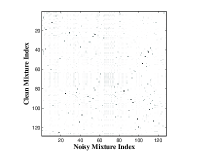
(a) Separately built noisy and clean GMMs

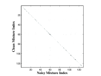
(b) GMMs of SPLICE and M-SPLICE

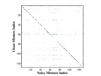
(c) Noisy GMM and MLLR-EM based clean GMM

Fig. 2: Mixture assignment distribution plots for Aurora-2 stereo training data

In this section, we motivate how M-SPLICE can be extended to datasets which are not stereo recorded. However some noisy training utterances, which are not necessarily the stereo counterparts of the clean data, are required.

4.1 Motivation

Consider a stereo dataset of $N$ training frames $(\mathbf{x}_{n},\mathbf{y}_{n})$. Suppose two $M$ mixture GMMs $p(\mathbf{x})$ and $p(\mathbf{y})$ are independently built using $\{\mathbf{x}_{n}\}$ and $\{\mathbf{y}_{n}\}$ respectively, and each data point is hard-clustered to the mixture giving the highest probability. We are interested in analysing a matrix $\mathbf{V}_{M\times M}$, built as

$$\mathbf{V}_{ij}=\sum_{n=1}^{N}\mathbbm{1}\left(\mathbf{x}_{n}\in i,\mathbf{y}_{n}\in j\right)$$

where $\mathbbm{1()}$ is indicator function. In other words, while parsing the stereo training data, when a stereo pair with clean part belonging to $i^{th}$ clean mixture and noisy part to $j^{th}$ noisy mixture is encountered, the $ij^{th}$ element of the matrix is incremented by unity. Thus each $ij^{th}$ element of the matrix denotes the number of stereo pairs belong to the $i^{th}$ clean $-$ $j^{th}$ noisy mixture-pair. When data are soft assigned to all the mixtures, the matrix can instead be built as:

$$\mathbf{V}_{ij}=\sum_{n=1}^{N}p(i\,|\,\mathbf{x}_{n})p(j\,|\,\mathbf{y}_{n})$$

Figure 2a visualises such a matrix built using Aurora-2 stereo training data using $128$ mixture models. A dark spot in the plot represents a higher data count, and a bulk of stereo data points do belong to that mixture-pair.

In conventional SPLICE and M-SPLICE, only the noisy GMM $p(\mathbf{y})$ is built, and not $p(\mathbf{x})$. $p\left(m\,|\,\mathbf{y}_{n}\right)$ are computed for every noisy frame, and the same alignments are assumed for the clean frames $\{\mathbf{x}_{n}\}$ while computing $\mathbf{\mu}_{x,m}$ and $\Sigma_{x,m}$. Hence $\mathbf{\mu}_{x,m}$, $\Sigma_{x,m}$ and $p\left(m\,|\,\mathbf{y}\right)$ can be considered as the parameters of a clean hypothetical GMM $p(\mathbf{x})$. Now, given these GMMs $p(\mathbf{y})$ and $p(\mathbf{x})$, the matrix $\mathbf{V}$ can be constructed, which is visualised in Figure (2b). Since the alignments are same, and $i^{th}$ clean mixture corresponds to the $i^{th}$ noisy mixture, a diagonal pattern can be seen.

Thus, under the assumption of Eq. (6), conventional SPLICE and M-SPLICE are able to estimate transforms from $i^{th}$ noisy mixture to exactly $i^{th}$ clean mixture by maintaining the mixture-correspondence.

When stereo data is not available, such exact mixture correspondence do not exist. Figure 2a makes this fact evident, since stereo property was not used while building the two independent GMMs. However, a sparse structure can be seen, which suggests that for most noisy mixtures $j$, there exists a unique clean mixture $i^{*}$ having highest mixture-correspondence. This property can be exploited to estimate piecewise linear transformations from every mixture $j$ of $p(\mathbf{y})$ to a single mixture $i^{*}$ of $p(\mathbf{x})$, ignoring all other mixtures $i\neq i^{*}$. This is the basis for the proposed extension to non-stereo data.

4.2 Implementation

In the absence of stereo data, our approach is to build two separate GMMs viz., clean and noisy during training, such that there exists mixture-to-mixture correspondence between them, as close to Fig. 2b as possible. Then whitening based transforms can be estimated from each noisy mixture to its corresponding clean mixture. This sort of extension is not obvious in the conventional SPLICE framework, since it is not straight-forward to compute the cross-covariance terms $\Sigma_{xy,m}$ without using stereo data. Also, M-SPLICE is expected to work better than SPLICE due to its advantages described earlier.

The training approach of two mixture-corresponded GMMs is as follows:

1. After building the noisy GMM $p(\mathbf{y})$, it is mean adapted by estimating a global MLLR transformation using clean training data. The transformed GMM has the same covariances and weights, and only means are altered to match the clean data. By this process, the mixture correspondences are not lost.

2. However, the transformed GMM need not model the clean data accurately. So a few steps of expectation maximisation (EM) are performed using clean training data, initialising with the transformed GMM. This adjusts all the parameters and gives a more accurate representation of the clean GMM $p(\mathbf{x})$.

Now, the matrix $\mathbf{V}$ obtained through this method using Aurora-2 training data is visualised in Figure 2c. It can be noted that no stereo information has been used while obtaining $p(\mathbf{x})$, following the above mentioned steps, from $p(\mathbf{y})$. It can be observed that a diagonal pattern is retained, as in the case of M-SPLICE, though there are some outliers. Since stereo information is not used, only comparable performances can be achieved. Figure 1b shows the block diagram of estimating transformations of non-stereo method. The steps are summarised as follows:

1. Build noisy GMM $p(\mathbf{y})$ using noisy features $\{\mathbf{y}\}$. This gives $\mu_{y,m}$ and $\Sigma_{y,m}$.

2. Adapt the means of noisy GMM $p(\mathbf{y})$ to clean data $\{\mathbf{x}\}$ using global MLLR transformation.

3. Perform at least three EM iterations to refine the adapted GMM using clean data. This gives $p(\mathbf{x})$, thus $\mu_{x,m}$ and $\Sigma_{x,m}$.

4. Compute $\mathbf{C}_{m}$ and $\mathbf{d}_{m}$ using Eq. (15) and (16).

The testing process is exactly same as that of M-SPLICE, as explained in Section 3.2.

5 Additional Run-time Adaptation

To improve the performance of the proposed methods during run-time, GMM adaptation to the test condition can be done in both conventional SPLICE and M-SPLICE frameworks in a simple manner. Conventional MLLR adaptation on HMMs involves two-pass recognition, where the transformation matrices are estimated using the alignments obtained through first pass Viterbi-decoded output, and a final recognition is performed using the transformed models.

MLLR adaptation can be used to adapt GMMs in the context of SPLICE and M-SPLICE as follows:

1. Adapt the noisy GMM through a global MLLR mean transformation

   $$\mathbf{\mu}_{y,m}^{(a)}\leftarrow\mathbf{\mu}_{y,m}$$

2. Now, adjust the bias term in conventional SPLICE or M-SPLICE as

   $$\mathbf{d}_{m}^{(a)}=\mathbf{\mu}_{x,m}-\mathbf{C}_{m}\mathbf{\mu}_{y,m}^{(a)}$$ (17)

This method involves only simple calculation of alignments of the test data w.r.t. the noisy GMM, and doesn’t need Viterbi decoding. Clean mixture means $\mathbf{\mu}_{x,m}$ computed during training need to be stored. A separate global MLLR mean transform can be estimated using test utterances belonging to each noise condition. The steps for testing process for run-time compensation are summarised as follows:

Table 1: Results on Aurora-2 Database

Noise Level	Baseline	SPLICE	M-SPLICE	Non-Stereo Method
Clean	99.25	98.97	99.01	99.08
SNR 20	97.35	97.84	97.92	97.68
SNR 15	93.43	95.81	96.10	95.15
SNR 10	80.62	89.48	91.03	87.37
SNR 5	51.87	72.71	77.59	68.49
SNR 0	24.30	42.85	50.72	39.00
SNR -5	12.03	18.52	22.27	16.73
Test A	67.45	81.39	83.47	77.44
Test B	72.26	83.24	84.18	79.63
Test C	68.14	69.42	78.06	73.54
Overall	69.51	79.74	82.67	77.54

(a) Comparison of SPLICE, M-SPLICE and non-stereo methods

MLLR (39)	SPLICE + Run-time Adaptation	M-SPLICE + Run-time Adaptation	Non-Stereo Method + Run-time Adaptation
99.28	99.05	99.02	99.08
98.33	97.96	98.18	97.77
96.82	96.21	96.87	95.47
91.88	90.61	93.10	88.80
73.88	75.05	82.00	72.36
41.94	46.27	57.51	44.98
18.71	20.10	27.32	20.43
79.31	82.45	86.47	80.12
82.55	84.09	85.91	81.67
79.14	73.01	82.90	75.79
80.57	81.22	85.53	79.88

(b) Comparison of adaptation methods

Table 2: Results on Aurora-4 Database

		Clean	Car	Babble	Street	Restaurant	Airport	Station	Average
Baseline	Mic-1	87.63	75.58	52.77	52.83	46.53	56.38	45.30	54.73
	Mic-2	77.40	64.39	45.15	42.03	36.26	47.69	36.32
Non-Stereo Method	Mic-1	86.85	77.71	62.62	58.96	55.93	61.95	55.37	61.66
	Mic-2	79.10	68.58	55.24	51.67	45.88	55.45	47.88

1. For all test vectors $\{\mathbf{y}\}$ belonging to a particular environment, compute the alignments w.r.t. the noisy GMM, i.e., $p(m\,|\,\mathbf{y})$.

2. Estimate a global MLLR mean transformation using $\{\mathbf{y}\}$, maximising the likelihood w.r.t. $p(\mathbf{y})$.

3. Compute the adapted noisy GMM $p^{(a)}(\mathbf{y})$ using the estimated MLLR transform. Only the means $\mathbf{\mu}_{y,m}$ of the noisy GMM would have been adapted as $\mathbf{\mu}_{y,m}^{(a)}$.

4. Using Eq. (17), recompute the bias term of SPLICE or M-SPLICE.

5. Compute the cleaned test vectors as

   $$\widehat{\mathbf{x}}=\sum_{m=1}^{M}p\left(m\,|\,\mathbf{y}\right)\left(\mathbf{C}_{m}\mathbf{y}+\mathbf{d}_{m}^{(a)}\right)$$

6 Experimental Setup

Aurora-2 task of 8 kHz sampling frequency [8] has been used to perform comparative study of the proposed techniques with the existing ones. Aurora-2 consists of connected spoken digits with stereo training data. The test set consists of utterances of ten different environments, each at seven distinct SNR levels. The acoustic word models for each digit have been built using left to right continuous density HMMs with 16 states and 3 diagonal covariance Gaussian mixtures per state. HMM Toolkit (HTK) 3.4.1 has been used for building and testing the acoustic models.

All SPLICE based linear transformations have been applied on 13 dimensional MFCCs, including $C_{0}$. During HMM training, the features are appended with 13 delta and 13 acceleration coefficients to get a composite 39 dimensional vector per frame. Cepstral mean subtraction (CMS) has been performed in all the experiments. 128 mixture GMMs are built for all SPLICE based experiments. Run-time noise adaptation in SPLICE framework is performed on 13 dimensional MFCCs. Data belonging to each SNR level of a test noise condition has been separately used to compute the global transformations. In all SPLICE based experiments, pseudo-cleaning of clean features has been performed.

To test the efficacy of non-stereo method on a database which doesn’t contain stereo data, Aurora-4 task of 8 kHz sampling frequency has been used. Aurora-4 is a continuous speech recognition task with clean and noisy training utterances (non-stereo) and test utterances of 14 environments. Aurora-4 acoustic models are built using crossword triphone HMMs of 3 states and 6 mixtures per state. Standard WSJ0 bigram language model has been used during decoding of Aurora-4. Noisy GMM of 512 mixtures is built for evaluating non-stereo method, using 7138 utterances taken from both clean and multi-training data. This GMM is adapted to standard clean training set to get the clean GMM.

6.1 Results

Tables 1a and 1b summarise the results of various algorithms discussed, on Aurora-2 dataset. All the results are shown in % accuracy. All SNRs levels mentioned are in decibels. The first seven rows report the overall results on all 10 test noise conditions. The rest of the rows report the average values in the SNR range 20-0 dB. Table 2 shows the experimental results on Aurora-4 database.

For reference, the result of standard MLLR adaptation on HMMs [9] has been shown in Table 1b, which computes a global 39 dimensional mean transformation, and uses two-pass Viterbi decoding.

It can be seen that M-SPLICE improves over SPLICE at all noise conditions and SNR levels and gives an absolute improvement of $8.6\%$ in test-set C and $2.93\%$ overall. Run-time compensation in SPLICE framework gives improvements over standard MLLR in test-sets A and B, whereas M-SPLICE gives improvements in all conditions. Here $9.89\%$ absolute improvement can be observed over SPLICE with run-time noise adaptation, and $4.96\%$ over standard MLLR. Finally, non-stereo method, though not using stereo data, shows $10.37\%$ and $6.93\%$ absolute improvements over Aurora-2 and Aurora-4 baseline models respectively, and a slight degradation w.r.t. SPLICE in all test cases. Run-time noise adaptation results of non-stereo method are comparable to that of standard MLLR, and are computationally less expensive.

7 Discussion

In terms of computational cost, the methods M-SPLICE and non-stereo methods are identical during testing as compared to conventional SPLICE. Also, there is almost negligible increase in cost during training. The MLLR mean adaptation in both non-stereo method and run-time adaptation are computationally very efficient, and do not need Viterbi decoding.

In terms of performance, M-SPLICE is able to achieve good results in all cases without any use of adaptation data, especially in unseen cases. In non-stereo method, one-to-one mixture correspondence between noise and clean GMMs is assumed. The method gives slight degradation in performance. This could be attributed to neglecting the outlier data.

Comparing with other existing feature normalisation techniques, the techniques in SPLICE framework operate on individual feature vectors, and no estimation of parameters is required from test data. So these methods do not suffer from test data insufficiency problems, and are advantageous for shorter utterances. Also, the testing process is usually faster, and are easily implementable in real-time applications. So by extending the methods to non-stereo data, we believe that they become more useful in many applications.

8 Conclusion and Future Work

A modified version of the SPLICE algorithm has been proposed for noise robust speech recognition. It is better compliant with the assumptions of SPLICE, and improves the recognition in highly mismatched and unseen noise conditions. An extension of the methods to non-stereo data has been presented. Finally, a convenient run-time adaptation framework has been explained, which is computationally much cheaper than standard MLLR on HMMs. In future, we would like to improve the efficiency of non-stereo extensions of SPLICE, and extend M-SPLICE in uncertainty decoding framework.

References

- [1] J. Droppo and A. Acero, “Maximum mutual information splice transform for seen and unseen conditions.,” in INTERSPEECH, pp. 989–992, 2005.
- [2] Y. Shinohara, T. Masuko, and M. Akamine, “Feature enhancement by speaker-normalized splice for robust speech recognition,” in Acoustics, Speech and Signal Processing (ICASSP), IEEE International Conference on, pp. 4881–4884, IEEE, 2008.
- [3] J. Droppo, A. Acero, and L. Deng, “Uncertainty decoding with splice for noise robust speech recognition,” in Acoustics, Speech, and Signal Processing (ICASSP), 2002 IEEE International Conference on, vol. 1, pp. I–57, IEEE, 2002.
- [4] K. Chijiiwa, M. Suzuki, N. Minematsu, and K. Hirose, “Unseen noise robust speech recognition using adaptive piecewise linear transformation,” in Acoustics, Speech and Signal Processing (ICASSP), IEEE International Conference on, pp. 4289–4292, IEEE, 2012.
- [5] J. Gonzalez, A. Peinado, A. Gomez, and J. Carmona, “Efficient MMSE estimation and uncertainty processing for multienvironment robust speech recognition,” Audio, Speech, and Language Processing, IEEE Transactions on, vol. 19, no. 5, pp. 1206–1220, 2011.
- [6] M. Afify, X. Cui, and Y. Gao, “Stereo-based stochastic mapping for robust speech recognition,” IEEE Trans. on Audio, Speech and Lang. Proc., vol. 17, pp. 1325–1334, Sept. 2009.
- [7] L. Deng, A. Acero, M. Plumpe, and X. Huang, “Large-vocabulary speech recognition under adverse acoustic environments,” in International Conference on Spoken Language Processing, pp. 806–809, 2000.
- [8] H.-G. Hirsch and D. Pearce, “The aurora experimental framework for the performance evaluation of speech recognition systems under noisy conditions,” in Automatic Speech Recognition: Challenges for the new Millenium ISCA Tutorial and Research Workshop (ITRW), 2000.
- [9] M. J. Gales, “Maximum likelihood linear transformations for hmm-based speech recognition,” Computer speech & language, vol. 12, no. 2, pp. 75–98, 1998.