KK MC 4.22: CEEX EW Corrections for $f\bar{f}\rightarrow f^{\prime}\bar{f^{\prime}}$ at LHC and Muon Colliders

Abstract

We present the upgrade of the coherent exclusive (CEEX) exponentiation realization of the Yennie-Frautschi-Suura (YFS) theory used in our Monte Carlo (${\cal KK}$ MC) to the processes $f\bar{f}\rightarrow f^{\prime}\bar{f^{\prime}},f=\mu,\tau,q,\nu_{\ell},f^{\prime}=e,\mu,\tau,q,\nu_{\ell},q=u,d,s,c,b,t,\ell=e,\mu,\tau$ with $f\neq f^{\prime}$, with an eye toward the precision physics of the LHC and possible high energy muon colliders. We give a brief summary of the CEEX theory in comparison to the older (EEX) exclusive exponentiation theory and illustrate theoretical results relevant to the LHC and possible muon collider physics programs.

I Introduction

Given that the era of precision QCD at the LHC is upon us, by which we mean theoretical precision tags at or below 1% in QCD corrections to LHC physical processes, computation of higher order EW corrections are also required: in the single $Z$ production process at the LHC for example, a u quark anti-u quark annihilation hard process at the Z pole has a radiation probability strength factor of $\frac{4}{9}\frac{2\alpha}{\pi}\left(\ln(M_{Z}^{2}/m_{u}^{2})-1\right)\cong 0.038$ if we use the value $m_{u}\cong 5.0$ MeV, the current quark mass value – we return to the best choice for the quark masses below. Evidently, we have to take these EW effects into account at the per mille level if we do not wish that they spoil the sub-1% precision QCD we seek in LHC precision QCD studies bflw1 . Indeed, when the cut on the respective energy of the emitted photons is at $v_{min}$ in units of the reduced cms effective beam energy, the $0.038$ strength factor above is enhanced to $0.038\ln(1/v_{min})$ and can easily become ${\cal O}(1)$. This means we have to use resummation, realized by MC event generator methods, of the type we have pioneered in Refs. eex to make contact with observation based on arbitrary cuts in any precise way. We call the reader’s attention here to the approaches of Refs. dima ; hor ; fewz ; den-ditt ; wac to EW corrections to such heavy gauge boson production at the LHC. It is well-known from LEP studies lepewwg that using only the exact ${\cal O}(\alpha)$ EW corrections is inadequate for per mille level accuracy on these corrections. Our studies below will show that this is still the case. This means that the approaches in Ref. dima ; fewz ; wac ; den-ditt must be extended to higher orders for precision LHC studies. We comment further below on the relation of our approach to that in Ref. hor as well.

Presently, we recall that in the case of single Z/$\gamma*$ production in high energy $e^{+}e^{-}$ annihilation our state of the art realization of such resummation is the CEEX YFS yfs ; ceex1 exponentiation we have realized by MC methods in the ${\cal KK}$ MC in Ref. kkmc . We conclude that we therefore need to extend the incoming states that the ${\cal KK}$ MC allows to include the incoming quarks and anti-quarks in the protons colliding at the LHC. Previous versions of ${\cal KK}$ MC even though not adapted for the LHC were already found useful in estimations of theoretical systematic errors of other calculations zwad1 ; zwad2 . We denote the new version of ${\cal KK}$ MC by version number 4.22, ${\cal KK}$ MC 4.22. Our aims in the current discussion in its regard are to summarize briefly on the main features of YFS/CEEX exponentiation ceex1 ; ceex2 in the SM EW theory, as this newer realization of the YFS theory is not a generally familiar one, to discuss the changes required to extend the incoming beam choices in the ${\cal KK}$ MC from the original $e^{+}e^{-}$ incoming state in Ref. kkmc to the more inclusive choices $f\bar{f},\;f=e,\mu,\tau,q,\nu_{\ell},\;q=u,d,s,b,\;\ell=e,\mu,\tau$, and to present examples of theoretical results relevant for the LHC and possible muon collider muclldr precision physics programs. For example, the muon collider physics program involves precision studies of the properties of the recently discovered BEH boson beh candidate atlas1 ; cms1 and treatment of the effects of higher order EW corrections will be essential to the success of the program, as we illustrate below.

In the next section, we review the older EEX exclusive realization and summarize the newer CEEX exclusive realization of the YFS yfs resummation in the SM EW theory; for, the YFS resummation is not generally familiar so that our review of the material in Refs. eex ; ceex1 ; ceex2 will aid the unfamiliar reader to follow the current discussion. We do this in the context of $e^{+}e^{-}$ annihilation physics programs for definiteness for historical reasons. In this way we illustrate the latter’s advantages over the former, which is also very successful. We also stress the key common aspects of our MC implementations of the two approaches to exponentiation, such as the exact treatment of phase space in both cases, the strict realization of the factorization theorem, etc. We stress that both of the realizations of YFS exponentiation are available in the ${\cal KK}$ MC 4.22 where both allow for the new incoming beams choices. This gives us important cross-check avenues required to establish the final precision tag of our results. In Sect. 3, we discuss and illustrate the extension of the choices of the incoming beams in the ${\cal KK}$ MC realization of CEEX/EEX. We illustrate results which quantify the size of the EW higher order corrections in LHC and muon collider physics scenarios. Specific realizations of the results we present here in the context of a parton shower environment will appear elsewhere elsewh . Sect. 4 contains our summary. Appendix 1 contains a sample output.

II Review of Standard Model calculations for $e^{+}e^{-}$ annihilation with YFS exponentiation

There are many examples of successful applications eex of our approach to the MC realization of the YFS theory of exponentiation for $e^{+}e^{-}$ annihilation physics: (1), for $e^{+}e^{-}\to f\bar{f}+n\gamma$, $f=\tau,\mu,d,u,s,c$ there are YFS1 (1987-1989) ${\cal O}(\alpha^{1})_{exp}$ ISR, YFS2$\in$KORALZ (1989-1990), ${\cal O}(\alpha^{1}+h.o.LL)_{exp}$ ISR, YFS3$\in$KORALZ (1990-1998), ${\cal O}(\alpha^{1}+h.o.LL)_{exp}$ ISR+FSR, and ${\cal KK}$ MC (98-02) ${\cal O}(\alpha^{2}+h.o.LL)_{exp}$ ISR+FSR+IFI with $d\sigma/\sigma=0.2\%$; (2), for $e^{+}e^{-}\to e^{+}e^{-}+n\gamma$ for $\theta<6^{\circ}$ there are BHLUMI 1.x, (1987-1990), ${\cal O}(\alpha^{1})_{exp}$ and BHLUMI 2.x,4.x, (1990-1996), ${\cal O}(\alpha^{1}+h.o.LL)_{exp}$ with $d\sigma/\sigma=0.061\%$; (3), for $e^{+}e^{-}\to e^{+}e^{-}+n\gamma$ for $\theta>6^{\circ}$ there is BHWIDE (1994-1998), ${\cal O}(\alpha^{1}+h.o.LL)_{exp}$ with $d\sigma/\sigma=0.2(0.5)\%$ at the Z peak ( just off the Z peak ); (4), for $e^{+}e^{-}\to W^{+}W^{-}+n\gamma$, $W^{\pm}\to f\bar{f}$ there is KORALW (1994-2001); and, (5), for $e^{+}e^{-}\to W^{+}W^{-}+n\gamma$, $W^{\pm}\to f\bar{f}$ there is YFSWW3 (1995-2001), YFS exponentiation + Leading Pole Approximation with $d\sigma/\sigma=0.4\%$ at LEP2 energies above the WW threshold. The typical MC realization we effect in Refs. eex is in the form of the “matrix element $\times$ exact phase space” principle, as we illustrate in the following diagram:

In practice it means the following:

• The universal exact Phase-space MC simulator is a separate module producing “raw events” (with importance sampling).

• The library of several types of SM/QED matrix elements which provides the “model weight” is another independent module ( the ${\cal KK}$MC example is shown).

• Tau decays and hadronization come afterwards of course.

The main steps in YFS exponentiation are the reorganization of the perturbative complete ${\cal O}(\alpha^{\infty})$ series such that IR-finite $\bar{\beta}$ components are isolated (factorization theorem) and the truncation of the IR-finite $\bar{\beta}$s to finite ${\cal O}(\alpha^{n})$ with the attendant calculation of them from Feynman diagrams recursively. We illustrate here the respective factorization for overlapping IR divergences for the 2$\gamma$ case – $R_{12}\in R_{1}$ and $R_{12}\in R_{2}$ as they are shown in the following picture:

$D_{0}(p_{f_{1}},p_{f_{2}},p_{f_{3}},p_{f_{4}})=\bar{\beta}_{0}(p_{f_{1}},p_{f_{2}},p_{f_{3}},p_{f_{4}});\\ ~{}~{}~{}~{}~{}~{}p_{f_{1}}+p_{f_{2}}=p_{f_{3}}+p_{f_{4}}$
$D_{1}(p_{f};k_{1})=\bar{\beta}_{0}(p_{f})\tilde{S}(k_{1})+\bar{\beta}_{1}(p_{f};k_{1});\\ ~{}~{}~{}~{}~{}~{}p_{f_{1}}+p_{f_{2}}\neq p_{f_{3}}+p_{f_{4}}$
$D_{2}(k_{1},k_{2})=\bar{\beta}_{0}\tilde{S}(k_{1})\tilde{S}(k_{2})+\bar{\beta}_{1}(k_{1})\tilde{S}(k_{2})+\bar{\beta}_{1}(k_{2})\tilde{S}(k_{1})+\bar{\beta}_{2}(k_{1},k_{2})$.
Note: $\bar{\beta}_{0}$ and $\bar{\beta}_{1}$ are used beyond their usual (Born and $1\gamma$) respective phase spaces. A kind of smooth “extrapolation” or “projection” is always necessary. We see that a recursive order-by-order calculation of the IR-finite $\bar{\beta}$s to a given fixed ${\cal O}(\alpha^{n})$ is possible: specifically,
$\bar{\beta}_{0}(p_{f_{1}},p_{f_{2}},p_{f_{3}},p_{f_{4}})=D_{0}(p_{f_{1}},p_{f_{2}},p_{f_{3}},p_{f_{4}})$,
$\bar{\beta}_{1}(p_{f};k_{1})=D_{1}(p_{f};k_{1})-\bar{\beta}_{0}(p_{f})\tilde{S}(k_{1})$,
$\bar{\beta}_{2}(k_{1},k_{2})=D_{2}(k_{1},k_{2})-\bar{\beta}_{0}\tilde{S}(k_{1})\tilde{S}(k_{2})-\bar{\beta}_{1}(k_{1})\tilde{S}(k_{2})-\bar{\beta}_{1}(k_{2})\tilde{S}(k_{1})$, $\ldots$, allow such a truncation.

In the classic EEX/YFS schematically the $\beta$’s are truncated to ${\cal O}(\alpha^{1})$, in the ISR example. For $e^{-}(p_{1},\lambda_{1})+e^{+}(p_{2},\lambda_{2})\to f(q_{1},\lambda^{\prime}_{1})+\bar{f}(q_{2},\lambda^{\prime}_{2})+\gamma(k_{1},\sigma_{1})+...+\gamma(k_{n},\sigma_{n})$, we have

$$\sigma=\sum\limits_{n=0}^{\infty}\;\;\int\limits_{m_{\gamma}}d\Phi_{n+2}\;e^{Y(m_{\gamma})}D_{n}(q_{1},q_{2},k_{1},...,k_{n})$$ (1)

with

$$\begin{split}&D_{0}=\bar{\beta}_{0},\qquad D_{1}(k_{1})=\bar{\beta}_{0}\tilde{S}(k_{1})+\bar{\beta}_{1}(k_{1}),\\ &D_{2}(k_{1},k_{2})=\bar{\beta}_{0}\tilde{S}(k_{1})\tilde{S}(k_{2})+\bar{\beta}_{1}(k_{1})\tilde{S}(k_{2})+\bar{\beta}_{1}(k_{2})\tilde{S}(k_{1}),\\ &D_{n}(k_{1},k_{2}...k_{n})=\bar{\beta}_{0}\tilde{S}(k_{1})\tilde{S}(k_{2})...\tilde{S}(k_{n})\\ &~{}+\bar{\beta}_{1}(k_{1})\tilde{S}(k_{2})\tilde{S}(k_{3})...\tilde{S}(k_{n})+\tilde{S}(k_{1})\bar{\beta}_{1}(k_{2})\tilde{S}(k_{3})...\tilde{S}(k_{n})\\ &~{}+...+\tilde{S}(k_{1})\tilde{S}(k_{2})\tilde{S}(k_{3})...\bar{\beta}_{1}(k_{n}).\end{split}$$ (2)

The real soft factors and the IR-finite building blocks are

$$\begin{split}&\tilde{S}(k)=\sum\limits_{\sigma}|{\mathfrak{s}}_{\sigma}(k)|^{2}=|{\mathfrak{s}}_{+}(k)|^{2}+|{\mathfrak{s}}_{-}(k)|^{2}\\ &~{}~{}~{}~{}~{}~{}~{}~{}~{}~{}~{}~{}~{}=-{\alpha\over 4\pi^{2}}\big{(}{q_{1}\over kq_{1}}-{q_{2}\over kq_{2}}\big{)}^{2}\\ &\bar{\beta}_{0}=(e^{-2\alpha\Re B_{4}}\sum_{\lambda}|{\mathcal{M}}^{\rm Born+Virt.}_{\lambda}|^{2})\big{|}_{{}_{{\cal O}(\alpha^{1})}},\\ &\bar{\beta}_{1}(k)=\sum\limits_{\lambda\sigma}|{\mathcal{M}}^{\rm 1-PHOT}_{\lambda\sigma}|^{2}-\sum\limits_{\sigma}|{\mathfrak{s}}_{\sigma}(k)|^{2}\sum\limits_{\lambda}|{\mathcal{M}}^{\rm Born}_{\lambda}|^{2},\end{split}$$ (3)

with $\lambda$ = fermion helicity, $\sigma$ = photon helicity, and everything being in terms of $\sum_{spin}|...|^{2}$!

The newer CEEX replaces older the EEX, where both are derived from the YFS theory yfs : EEX, Exclusive EXponentiation, is very close to the original Yennie-Frautschi-Suura formulation, which is also now featured in the MC’s Herwig++ hw++ and Sherpa shpa for particle decays. We need to stress that CEEX, Coherent EXclusive exponentiation, is an extension of the YFS theory. Because of its coherence CEEX is friendly to quantum coherence among the Feynman diagrams, so that we have the complete $|\sum_{diagr.}^{n}{\mathcal{M}}_{i}\big{|}^{2}$ rather than the often incomplete $\sum_{i,j}^{n^{2}}{\mathcal{M}}_{i}{{\mathcal{M}}_{j}}^{*}$. It follows that we get readily the proper treatment of narrow resonances, $\gamma\oplus Z$ exchanges, $t\oplus s$ channels, ISR$\oplus$FSR, angular ordering, etc. KORALZ/YFS2, BHLUMI, BHWIDE, YFSWW, KoralW and KORALZ are examples of the EEX formulation in our MC event generator approach; ${\cal KK}$MC is the only example of the CEEX formulation.

Using the example of ISR ${\cal O}(\alpha^{1})$ we illustrate CEEX schematically for the process $e^{-}(p_{1},\lambda_{1})+e^{+}(p_{2},\lambda_{2})\to f(q_{1},\lambda^{\prime}_{1})+\bar{f}(q_{2},\lambda^{\prime}_{2})+\gamma(k_{1},\sigma_{1})+...+\gamma(k_{n},\sigma_{n}).$ We have

$$\begin{split}&\sigma=\sum\limits_{n=0}^{\infty}\;\int_{m_{\gamma}}d\Phi_{n+2}\!\!\!\!\sum\limits_{\lambda,\sigma_{1},...,\sigma_{n}}\!\!\!\!|e^{\alpha B(m_{\gamma})}{\mathcal{M}}^{\lambda}_{n,\sigma_{1},...,\sigma_{n}}(k_{1},...,k_{n})|^{2},\qquad{\mathcal{M}}_{0}^{\lambda}=\hat{\beta}_{0}^{\lambda},\quad{\mathcal{M}}^{\lambda}_{1,\sigma_{1}}(k_{1})=\hat{\beta}^{\lambda}_{0}{\mathfrak{s}}_{\sigma_{1}}(k_{1})+\hat{\beta}^{\lambda}_{1,\sigma_{1}}(k_{1}),\qquad\\ &{\mathcal{M}}^{\lambda}_{2,\sigma_{1},\sigma_{2}}(k_{1},k_{2})=\hat{\beta}^{\lambda}_{0}{\mathfrak{s}}_{\sigma_{1}}(k_{1}){\mathfrak{s}}_{\sigma_{2}}(k_{2})+\hat{\beta}^{\lambda}_{1,\sigma_{1}}(k_{1}){\mathfrak{s}}_{\sigma_{2}}(k_{2})+\hat{\beta}^{\lambda}_{1,\sigma_{2}}(k_{2}){\mathfrak{s}}_{\sigma_{1}}(k_{1}),\qquad{\mathcal{M}}^{\lambda}_{n,\sigma_{1},...\sigma_{n}}(k_{1},...k_{n})=\hat{\beta}^{\lambda}_{0}{\mathfrak{s}}_{\sigma_{1}}(k_{1}){\mathfrak{s}}_{\sigma_{2}}(k_{2})...{\mathfrak{s}}_{\sigma_{n}}(k_{n})+\\ &+\hat{\beta}^{\lambda}_{1,\sigma_{1}}(k_{1}){\mathfrak{s}}_{\sigma_{2}}(k_{2})...{\mathfrak{s}}_{\sigma_{n}}(k_{n})+{\mathfrak{s}}_{\sigma_{1}}(k_{1})\hat{\beta}^{\lambda}_{1,\sigma_{2}}(k_{2})...{\mathfrak{s}}_{\sigma_{n}}(k_{n})+...+{\mathfrak{s}}_{\sigma_{1}}(k_{1}){\mathfrak{s}}_{\sigma_{2}}(k_{2})...{\mathfrak{s}}_{\sigma_{n-1}}(k_{n-1})\hat{\beta}^{\lambda}_{1,\sigma_{n}}(k_{n}),\end{split}$$ (4)

where $\lambda$ is the collective index of fermion helicities. The ${\cal O}(\alpha^{1})$ IR-finite building blocks are:

$$\begin{split}&\hat{\beta}^{\lambda}_{0}=\big{(}e^{-\alpha B_{4}}{\mathcal{M}}^{\rm Born+Virt.}_{\lambda}\big{)}\big{|}_{{\cal O}(\alpha^{1})},\\ &\hat{\beta}^{\lambda}_{1,\sigma}(k)={\mathcal{M}}^{\lambda}_{1,\sigma}(k)-\hat{\beta}^{\lambda}_{0}{\mathfrak{s}}_{\sigma}(k)\end{split}$$

Everything above is expressed in terms of ${\mathcal{M}}$-amplitudes! Distributions are $\geq 0$ by construction! In ${\cal KK}$MC the above is done up to ${\cal O}(\alpha^{2})$ for ISR and FSR.

The full scale CEEX ${\cal O}(\alpha^{r})$, r=1,2, master formula for the polarized total cross section reads as follows:

$$\begin{split}&\sigma^{(r)}\!=\!\!\sum_{n=0}^{\infty}{1\over n!}\int d\tau_{n}(p_{a}\!+\!p_{b};p_{c},p_{d},k_{1},\dots,k_{n})\\ &~{}\times e^{2\alpha\Re B_{4}}\!\sum_{\sigma_{i},\lambda,\bar{\lambda}}\;\sum_{i,j,l,m=0}^{3}\hat{\varepsilon}^{i}_{a}\hat{\varepsilon}^{j}_{b}\sigma^{i}_{\lambda_{a}\bar{\lambda}_{a}}\sigma^{j}_{\lambda_{b}\bar{\lambda}_{b}}\\ &~{}\times\mathfrak{M}^{(r)}_{n}\left({}^{p}_{\lambda}{}^{k_{1}}_{\sigma_{1}}{}^{k_{2}}_{\sigma_{2}}\dots{}^{k_{n}}_{\sigma_{n}}\right)\Big{[}\mathfrak{M}^{(r)}_{n}\!\left({}^{p}_{\bar{\lambda}}{}^{k_{1}}_{\sigma_{1}}{}^{k_{2}}_{\sigma_{2}}\dots{}^{k_{n}}_{\sigma_{n}}\right)\Big{]}^{\star}\sigma^{l}_{\bar{\lambda}_{c}\lambda_{c}}\sigma^{m}_{\bar{\lambda}_{d}\lambda_{d}}\hat{h}^{l}_{c}\hat{h}^{m}_{d}.\end{split}$$ (5)

The respective CEEX amplitudes are

$$\begin{split}\mathfrak{M}^{(1)}_{n}\left({}^{p}_{\lambda}{}^{k_{1}}_{\sigma_{1}}\dots{}^{k_{n}}_{\sigma_{n}}\right)\!&=\sum\limits_{\wp\in{\cal P}}\prod\limits_{i=1}^{n}{\mathfrak{s}}_{[i]}^{\{\wp_{i}\}}\Bigg{\{}\hat{\beta}_{0}^{(1)}\big{(}{}^{p}_{\lambda};X_{\wp}\big{)}\!+\sum\limits_{j=1}^{n}{\hat{\beta}^{(1)}_{1\{\wp_{j}\}}\big{(}{}^{p}_{\lambda}{}^{k_{j}}_{\sigma_{j}};X_{\wp}\big{)}\over{\mathfrak{s}}_{[j]}^{\{\wp_{j}\}}}\Bigg{\}}\\ \mathfrak{M}^{(2)}_{n}\left({}^{p}_{\lambda}{}^{k_{1}}_{\sigma_{1}}\dots{}^{k_{n}}_{\sigma_{n}}\right)&=\!\sum\limits_{\wp\in{\cal P}}\prod\limits_{i=1}^{n}{\mathfrak{s}}_{[i]}^{\{\wp_{i}\}}\Bigg{\{}\hat{\beta}_{0}^{(2)}\big{(}{}^{p}_{\lambda};X_{\wp}\big{)}\!+\!{\sum\limits_{j=1}^{n}}{\hat{\beta}^{(2)}_{1\{\wp_{j}\}}\big{(}{}^{p}_{\lambda}{}^{k_{j}}_{\sigma_{j}};X_{\wp}\big{)}\over{\mathfrak{s}}_{[j]}^{\{\wp_{j}\}}}\!+\!{\sum\limits_{1\leq j<l\leq n}}{\hat{\beta}^{(2)}_{2\{\wp_{j},\wp_{l}\}}\big{(}{}^{p}_{\lambda}{}^{k_{j}}_{\sigma_{j}}{}^{k_{l}}_{\sigma_{l}};X_{\wp}\big{)}\over{\mathfrak{s}}_{[j]}^{\{\wp_{j}\}}{\mathfrak{s}}_{[l]}^{\{\wp_{l}\}}}\Bigg{\}}.\end{split}$$ (6)

For the full details see ref. ceex1 .

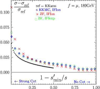
Figure 1: Principal cross checks of ${\cal KK}$MC for $e^{-}e^{+}\to\mu^{-}\mu^{+}+n\gamma$ process at $\sqrt{s}=$189GeV.

The precision tags of the ${\cal KK}$MC are determined by comparisons with our own semi-analytical and independent MC results and by comparison with the semi-analytical results of the program ZFITTER zfitter . In Fig. 1 we illustrate such comparisons, which lead to the ${\cal KK}$MC precision tag $d\sigma/\sigma=0.2\%$ for example. The ISR of ZFITTER is based on the ${\cal O}(\alpha^{2})$ result of ref. berends , while ${\cal KK}$MC is totally independent! See Ref. ceex1 ; recent2 for a more complete discussion. Thus, we know that ${\cal KK}$MC has the capability to deliver per mille precision on the large EW effects if it is extended to the appropriate incoming beams for the LHC and the muon collider. To this we now turn.

III Extension of ${\cal KK}$MC to the processes $f\bar{f}\to f^{\prime}\bar{f^{\prime}},$ $f=\mu,q,\nu_{\ell}$, $f^{\prime}=\ell,\nu_{\ell},q,q=u,d,s,c,b,$ $\ell=e,\mu,\tau,f\neq f^{\prime},$

At the LHC and at a futuristic muon collider muclldr , the incoming beams involve for $Z/\gamma*$ production and decay the other light charged fundamental fermions in the SM: $u,d,s,c,b$ for the LHC and the muon for a muon collider. Thus, we need to extend the matrix elements, residuals, and IR functions in (1,5) to the case where we substitute the $e^{-},\;e^{+}$ EW charges by the new beam particles $f,\;\bar{f}$ EW charges and we substitute the mass $m_{e}$ everywhere by $m_{f}$ . We have done this with considerable cross checks against the same semi-analytical tools that we employed in Ref. ceex1 to establish the precision tag of version 4.13 of ${\cal KK}$MC. We want to stress that this was a highly non-trivial set of cross-checks: for example, we found that the MC procedure used in the crude MC cross section was unstable when the value of the radiation strength factor $\gamma_{f}=\frac{2Q_{F}^{2}\alpha}{\pi}\left(\ln(s/m_{f}^{2})-1\right)$ becomes too small. This instability was removed and the correct value of the MC crude cross section was verified by semi-analytical methods. We did therefore a series of cross checks/illustrations with the new version of ${\cal KK}$MC, version 4.22, which we now exhibit.

Turning first to the most important cross-check, we show in Tab. 1 and Figs. 2-4 that for the $e^{+}e^{-}\rightarrow\mu^{+}\mu^{-}$ process, our new version ${\cal KK}$MC 4.22 reproduces the results in the corresponding $\sqrt{s}=189$GeV cross checks done in Ref. ceex1 for the dependence of the CEEX calculated cross section and $A_{FB}$ on the energy cut-off on $v=1-s^{\prime}/s$ where $s^{\prime}=M^{2}_{\mu\bar{\mu}}$ is the invariant mass of the $\mu\bar{\mu}$-system. The reader can check that the two sets of results, those given here in Tab. 1 and Figs. 2-4 and those given in Table 5, Figs. 20,21, and 18 in Ref. ceex1 are in complete agreement within statistical fluctuations. This shows that our introduction of the new beams has not spoiled the precision of the ${\cal KK}$MC for the incoming $e^{+}e^{-}$ state.

Table 1: Energy cut-off study of total cross section $\sigma$ and charge asymmetry $A_{\rm FB}$ for annihilation process $e^{-}e^{+}\to\mu^{-}\mu^{+}$, at $\sqrt{s}=$189GeV. Energy cut: $v<v_{\max}$, $v=1-M^{2}_{f\bar{f}}/s$. Scattering angle for $A_{\rm FB}$ is $\theta^{\bullet}$(defined in Phys. Rev. D41, 1425 (1990)). No cut in $\theta^{\bullet}$. E-W corr. in ${\cal KK}$  according to DIZET 6.x. In addition to CEEX matrix element, results are also shown for ${\cal O}(\alpha^{3})_{\rm LL}$ EEX3 matrix element without ISR$\otimes$FSR interf. ${\cal KK}$sem is semianalytical program, part of ${\cal KK}$MC.

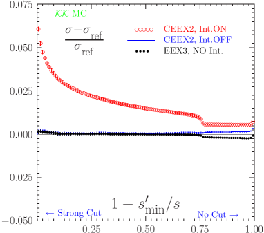
Figure 2: Total cross section $\sigma$, energy cut-off study. The same results as in the Table 1. Ref. $\sigma_{\rm ref}$ = semianalytical of ${\cal KK}$sem.

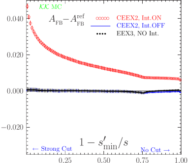
Figure 3: Energy cut-off study of charge asymmetry $A_{\rm FB}$ for the process $e^{+}e^{-}\to\mu^{+}\mu^{-}$. The same results as in the Table 1. Reference $A_{\rm FB}^{\rm ref}$ = semianalytical ${\cal KK}$sem.

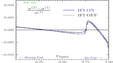
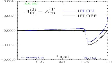
Figure 4: Physical precision of CEEX ISR matrix element for $e^{-}e^{+}\to\mu^{-}\mu^{+}$at $\sqrt{s}=$189GeV. See table 1 for definition of cut-offs.

We turn next to the new type of incoming beam scenario in Tab. 2 and Figs. 5-7 wherein we show the analogous results to those in Tab. 1 and Figs. 2-4 for the process $d\bar{d}\rightarrow\mu^{-}\mu^{+}$ at $\sqrt{s}=189$GeV so that we can keep a good reference to the relative size of the EW corrections versus what one would have in the usual $e^{+}e^{-}$ annihilation case. We see that for strong cuts, with $v_{max}\sim.01$ and for the loose cut, with $v_{max}\sim 0.99$, the effects are similar to those in the more familiar incoming $e^{+}e^{-}$ annihilation case, as the sign of the EW charges are the same for the $d$ and the $e^{-}$. The values are different so that size of the effects in Tab. 2 and Figs. 5-7 are correspondingly different. For example, in the strong cut, turning the initial-final state interference(IFI) off changes the CEEX cross section result for $v_{max}=0.01$ by $-1.9\%$ for the incoming $d\bar{d}$ case compared to $-5.9\%$ for the incoming $e^{-}e^{+}$ case. The behavior of $A_{FB}(v_{max})$ is similar between to the two incoming beam sets, where turning the IFI off reduces the value of $A_{FB}$ at $v_{max}=0.01$ by $8.12\%(2.55\%)$ respectively for the incoming $e^{-}e^{+}(d\bar{d})$ case. In both cases, the loose cut such as $v_{max}=0.99$ tends to wash-out these effects. In Fig. 5 the data on the cross sections in the table in Tab. 2 are plotted in relation to the reference semi-analytical result denoted as ${\cal KK}$sem ceex1 as the ratio of their difference to the reference divided by the reference and in Fig.6 the corresponding data on $A_{FB}$ are plotted as their difference with the respective ${\cal KK}$sem results. When compared to the analogous results for the usual $e^{-}e^{+}$ case in Figs. 2 and 3 we see that structure at the Z-radiative return position, $v_{mas}\cong 0.77$, is very much reduced in the $d\bar{d}$ case due to the smaller electric charge magnitude, just as the size of the IFI effects themselves are similarly reduced. In Fig. 7, we show the physical precision test which compares the size of the second and first order CEEX results for the cross section and the forward-backward asymmetry: for the $d\bar{d}$ case compared to the similar plots in Fig. 4 for the $e^{-}e^{+}$ case we see that for the strong cuts we have higher precision, we have smooth behavior through the Z-peak region, and that at the very loose cuts the two precision tags are similar, where we would estimate that similar value at $0.35\%$ in the worst case that $v_{max}\rightarrow 1$ on the cross section for example – here we use half the difference shown in the figure as the error estimate. For the more generic energy cut of $0.6\%$ our physical precision estimate is $0.05\%$. This is the type of precision required for the precision LHC physics studies.

Table 2: Study of total cross section $\sigma(v_{\max})$ and charge asymmetry $A_{\rm FB}(v_{\max})$, $d\bar{d}\to\mu^{-}\mu^{+}$, at $\sqrt{s}$ =189GeV. See Table 1 for definition of the energy cut $v_{\max}$, scattering angle and M.E. type,

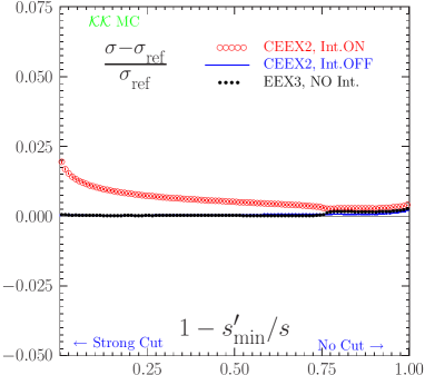
Figure 5: Energy cut-off study of Total cross section for $d\bar{d}\to\mu^{-}\mu^{+}$, at 189GeV. The same as in the table 2. $\sigma_{\rm ref}$ = semianalytical of ${\cal KK}$sem.

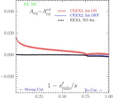
Figure 6: Energy cut-off study of charge asymmetry $A_{\rm FB}$ for the process $d\bar{d}\to\mu^{-}\mu^{+}$, at 189GeV. Reference $A_{\rm FB}^{\rm ref}$ from semianalytical ${\cal KK}$sem.

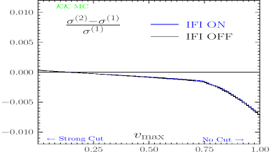
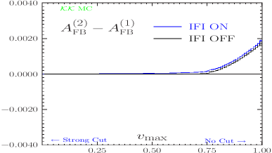
Figure 7: Physical precision of CEEX ISR matrix element for $d\bar{d}\to\mu^{-}\mu^{+}$at $\sqrt{s}=$189GeV. See table 1 for definition of cut-offs.

Turning next to the incoming $u\bar{u}$ case, we show in Tab. 3 and Figs. 8-10 the analogous results to those in Tab. 2 and Figs. 5-7 for the $u\bar{u}\rightarrow\mu^{-}\mu^{+}$ at $\sqrt{s}=189$GeV, so that again we have the reference to the usual incoming $e^{+}e^{-}$ annihilation case regarding the size and nature of the EW effects expected. We see that the effects are now quantitatively different, because the sizes of the EW charges are different, but they also have the opposite sign in the enhanced regions because the EW charges of the u quarks have the opposite sign to those of the $e^{-}$. This means that in the LHC environment in processes such as single $Z$ boson production there will be some compensation between the effects from u and d quarks. A detailed application of the new ${\cal KK}$MC two such scenarios will appear elsewhere. Here, we specifically note that for the strong cut case with $v_{max}=0.01$ the IFI effect on the cross section in Tab. 3 is $-4.14\%$ while the effect on $A_{FB}$ at this value of $v_{max}$ is $-3.52\%$, both of which correlate well with the value of the u-quark EW charges compared to the $e^{-}$ EW charges, where the corresponding results are from Tab. 1 $5.9\%$ and $8.12\%$ respectively. In Figs. 8 and 9 we show for the incoming $u\bar{u}$ the analogous plots to those in Figs. 5 and 6 for the incoming $d\bar{d}$ case of the relative values of the data in Tab. 3. We see that the structure at the Z-radiative return position is a bit more evident than for the latter case and that the IFI(Initial-Final state Interference) effects are correspondingly more evident in general, as expected. In Fig. 10, we show the corresponding physical precision study as the difference between the second and first order CEEX predictions. In the worst case scenario with $v_{max}\rightarrow 1$ we have the estimate at 0.5% on the cross section; at strong cuts $v_{max}\rightarrow 0$ we have $0.025\%$ and at moderate cuts near $v_{max}\cong 0.6$ we have $.08\%$, as needed for precision LHC studies. These estimates hold for both the IFI on and IFI off cases.

Table 3: Study of total cross section $\sigma(v_{\max})$ and charge asymmetry $A_{\rm FB}(v_{\max})$, $u\bar{u}\to\mu^{-}\mu^{+}$, at $\sqrt{s}$ =189GeV. See Table 1 for definition of the energy cut $v_{\max}$, scattering angle and M.E. type,

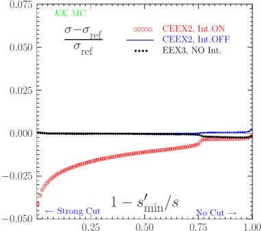
Figure 8: Total cross section $\sigma$, energy cut-off study for the process $u\bar{u}\to\mu^{+}\mu^{-}$. The same as in the table 3. No cut in $\theta^{\bullet}$. Ref. $\sigma_{\rm ref}$ = semianalytical of ${\cal KK}$sem.

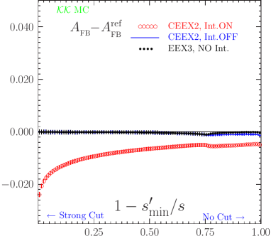
Figure 9: Charge asymmetry $A_{\rm FB}$, energy cut-off study for the process $u\bar{u}\to\mu^{+}\mu^{-}$. The same as in the table 3. No cut in $\theta^{\bullet}$.

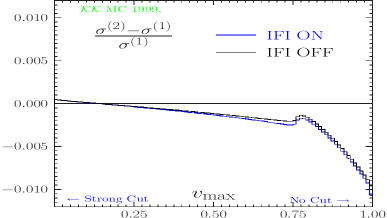
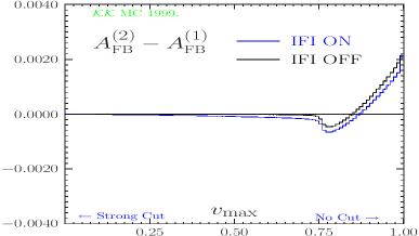
Figure 10: Physical precision of CEEX ISR matrix element for $u\bar{u}\to\mu^{-}\mu^{+}$at $\sqrt{s}=$189GeV. See table 1 for definition of cut-offs.

As most of the cross section at the LHC in the single $Z/\gamma*$ production and decay to lepton pairs is concentrated near the $Z-$resonance, we next turn to the similar studies as we have shown in Tabs. 1-3 and Figs. 2-10 for $\sqrt{s}=M_{Z}$ so see more directly what type of effects one has to consider in precision studies of these processes. We stress that with $25fb^{-1}$ of recorded data for each of ATLAS and CMS, the number of such decays exceeds 10 M in each experiment. Turning first to the $d\bar{d}$ incoming beam scenario we have the results in Tab. 4 and Figs. 11-13. We see that the small width(that is to say the lifetime) of the Z suppresses the IFI effects as expected: on the cross section even for the strong cut $v_{max}=0.01$ the effect is at the level of only $0.065\%$ and it is already essentially non-existent at $v_{max}=0.1$; on $A_{FB}$ a $5.5\%$ enhancement at $v_{max}=0.01$ is already reduced to $0.29\%$ at $v_{max}=0.1$. But, the effect of the radiation on the cross section is quite pronounced, as the cross section changes by 26% between the strong cut $v_{max}=0.01$ and the loose cut $v_{max}=0.99$. Thus, high precision on its theoretical prediction is essential for LHC precision studies. Indeed, these remarks are borne out in the plots in Figs. 11 and 12, where we respectively see the closeness of the CEEX cross section with the IFI on and IFI off and the similar closeness of the CEEX forward-backward asymmetries with the IFI on and off except for the region below $v_{max}=0.01$, where the IFI effect reaches $5.5\%$. Turning to the physical precision study in Fig. 13, we see that in the typical scenario where $v_{max}\cong 0.6$, the precision tag for both IFI on and the IFI off cross sections is $0.04\%$, sufficient for the precision LHC studies.

Table 4: Study of total cross section $\sigma(v_{\max})$ and charge asymmetry $A_{\rm FB}(v_{\max})$, $d\bar{d}\to\mu^{-}\mu^{+}$, at $\sqrt{s}$ = 91.187GeV. See Table 1 for definition of the energy cut $v_{\max}$, scattering angle and M.E. type,

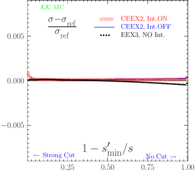
Figure 11: Total cross section $\sigma$, energy cut-off study for the process $d\bar{d}\to\mu^{-}\mu^{+}$ at the $Z$. Results the same as in the table 4.

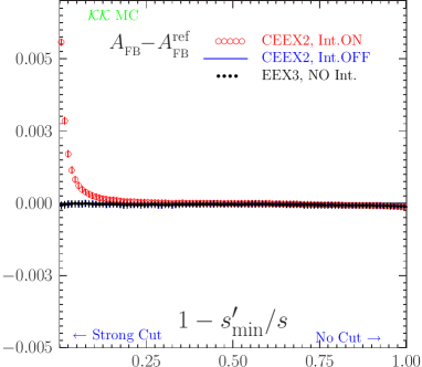
Figure 12: Charge asymmetry $A_{\rm FB}$, energy cut-off study for the process $d\bar{d}\to\mu^{-}\mu^{+}$ at the $Z$. Results the same as in the table 4.

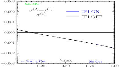
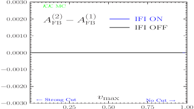
Figure 13: Physical precision of CEEX ISR matrix element for $d\bar{d}\to\mu^{-}\mu^{+}$at $\sqrt{s}=$ 91.187GeV. See table 1 for definition of cut-offs.

Continuing in this vein, we present next the incoming $u\bar{u}$ scenario at $\sqrt{s}=M_{Z}$ in Tab. 5 and Figs. 14-16. We see again that that the small width of the Z suppresses the IFI effects: the negative effects at $v_{max}=0.01$ of $-0.0587\%$ on the cross section and $-16.2\%$ on $A_{FB}$ become respectively non-existent and $-.989\%$ at $v_{max}=0.1$; at the loose cut $v_{max}=0.99$ the IFI effect on the cross section(the forward-backward asymmetry) is below the $0.01\%(0.00285)$ precision of the data. The cross section varies by $30.6\%$ as $v_{max}$ varies from $0.01$ to $0.99$ so again its theoretical prediction for the radiative effects must have high precision for precision studies. These remarks are borne out by the plots in Figs. 14 and 15, where see that the IFI on and IFI CEEX cross sections are very close to the reference cross section even for the very strong and loose cuts and that the IFI on and off CEEX forward-backward asymmetries are the same as the EEX3 value by an energy cut value of $0.25$, for example. In Fig. 16, we see the precision study shows that the cross section has the precision estimate of $0.04\%$ at the energy cut of $0.6$ just as we had for the incoming $d\bar{d}$ case. Again, this is sufficient for precision studies of LHC physics.

Table 5: Study of total cross section $\sigma(v_{\max})$ and charge asymmetry $A_{\rm FB}(v_{\max})$, $u\bar{u}\to\mu^{-}\mu^{+}$, at $\sqrt{s}$ = 91.187GeV. See Table 1 for definition of the energy cut $v_{\max}$, scattering angle and M.E. type,

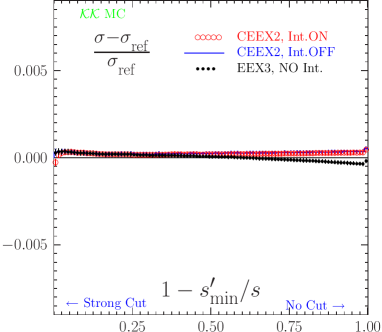
Figure 14: Total cross section $\sigma$, energy cut-off study for the process $u\bar{u}\to\mu^{+}\mu^{-}$ at the $Z$ peak. Results the same as in the table 5.

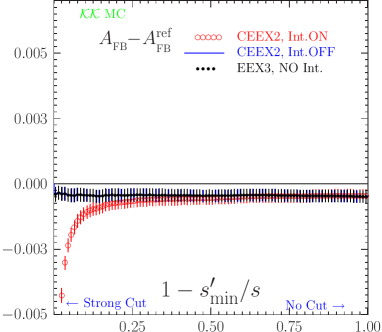
Figure 15: Charge asymmetry $A_{\rm FB}$, energy cut-off study for the process $u\bar{u}\to\mu^{-}\mu^{+}$ at the $Z$. Results the same as in the table 5.

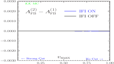
Figure 16: Physical precision of CEEX ISR matrix element for $u\bar{u}\to\mu^{-}\mu^{+}$at $\sqrt{s}=$ 91.187GeV($Z$ peak). See table 1 for definition of cut-offs.

While we have discussed the individual incoming $q\bar{q}$ scenarios, ${\cal KK}$MC 4.22 has a beamstrahlung option in which one may replace the beamstrahlung functions with the proton PDF’s. We have done this as a proof of principle exercise and we show in Appendix 1 the results of a simple test run at $7$TeV. What we see in this test run output is that indeed significant probability exists for the incoming quarks to radiate non-zero $p_{T}$ in the higher order corrections: these effects cannot be properly described by zero $p_{T}$ methods such as structure function techniques hor . We will return to such studies elsewhere elsewh .

Finally, given the interest in muon collider precision physics muclldr , we consider next the process $\mu^{+}\mu^{-}\rightarrow e^{+}e^{-}$ again at $\sqrt{s}=189$GeV, so that again we have the reference to the usual incoming $e^{+}e^{-}$ annihilation case regarding the size and nature of the EW effects expected. In this case we have all the same EW charges but the ISR probability to radiate factor $\gamma_{e}=\frac{2\alpha}{\pi}\left(\ln(s/m_{e}^{2})-1\right)\cong 0.114$ becomes $\gamma_{\mu}=\frac{2\alpha}{\pi}\left(\ln(s/m_{\mu}^{2})-1\right)\cong 0.0649$. This means that we expect the EW effects where the photonic corrections dominate to show reduction in size for ISR dominated regimes, the same size for the IFI dominated regimes. This is borne-out by the results in Tab. 6 and Figs. 17-19. In the regime of the strong cut, with $v_{max}=0.01$, the results are very similar in all aspects to the usual incoming $e^{-}e^{+}$ case: the cross section is enhanced by $6.0\%$ to be compared with $5.9\%$ and $A_{FB}$ is enhanced by $8.3\%$ to be compared to $8.1\%$. In the regime of the loose cut, with $v_{max}=0.99$, the cross section is enhanced by $0.49\%$ to be compared with $0.38\%$ and $A_{FB}$ is enhanced by $1.7\%$ to be compared to $2.4\%$. In Figs. 17 and 18 we see that we have same general behavior as we have in Figs. 2 and 3, the characteristic Z peak radiative return structure in Fig. 17 and its inflection behavior in Fig. 18. In Fig. 19, we see that the precision studies comparing the second order and first order CEEX results show the pronounced effect of the Z radiative return. At an energy cut of $0.6$, we see again that a precision tag of $0.2\%$ obtains, so that precision results for EW effects would be available. The detailed application of such results to muon collider physics will be taken up elsewhere elsewh2 .

Table 6: Study of total cross section $\sigma(v_{\max})$ and charge asymmetry $A_{\rm FB}(v_{\max})$, $\mu^{-}\mu^{+}\to e^{-}e^{+}$, at $\sqrt{s}$ = 189GeV. See Table 1 for definition of the energy cut $v_{\max}$, scattering angle and M.E. type,

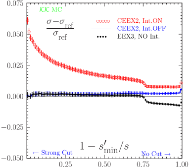
Figure 17: Energy cut-off study of total cross section for $\mu^{-}\mu^{+}\to e^{-}e^{+}$at energy 189GeV. The same results as in Table 6.

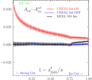
Figure 18: Energy cut-off study of total charge asymmetry for $\mu^{-}\mu^{+}\to e^{-}e^{+}$at energy 189GeV. The same results as in Table 6.

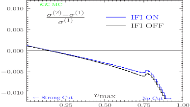
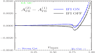
Figure 19: Physical precision of CEEX ISR matrix element for $\mu^{-}\mu^{+}\to e^{-}e^{+}$at $\sqrt{s}=$ 189GeV. See table 1 for definition of cut-offs.

IV Conclusions

YFS inspired EEX and CEEX MC schemes are successful examples of Monte Carlos based directly on the factorization theorem (albeit for the IR soft case for Abelian QED only). These schemes work well in practice: KORALZ, BHLUMI, YWSWW3, BHWIDE and ${\cal KK}$MC are examples. The extension of such schemes (as far as possible) to all collinear singularities would be very desirable and practically important! Work on this is in progress– see Refs. sjms ; herwiri1 ; herwiri2 for recent results and outlooks.

Here, we have illustrated that the ${\cal KK}$MC program is extended to the new incoming $f\bar{f},\;f=\mu,\tau,\nu_{\ell},q,\;q=u,d,s,c,b,\;\ell=e,\mu,\tau,$ beams cases. The quark-anti-quark and $\mu^{-}\mu^{+}$ incoming beam cases are respectively important for the LHC precision EW predictions at the per mille level and to the precision EW studies for the possible muon collider physics program. We have seen that in all cases, the per mille level accuracy requirements necessitate the implementation of the ${\cal KK}$MC class of EW higher order effects. Realizations and applications of this class of higher order EW effects is in progress and will appear elsewhere elsewh . The new version of the ${\cal KK}$MC, version 4.22, is available at https://jadach.web.cern.ch/jadach/KKindex.html

Acknowledgments
The authors thank Prof. I. Antoniadis for the support and kind hospitality of the CERN Theory Division while this work was in progress. They also thank Dr. S.A. Yost for useful discussions. One of the authors (S.J.) also thanks the Dean Lee Nordt of the Baylor College of Arts & Sciences for Baylor’s support while this work was in progress. This work is partly supported by the Polish National Science Centre grant DEC-2011/03/B/ST2/02632.

Appendix A Sample Monte Carlo events

Below sample output from run of ${\cal KK}$ MC version 4.22 is presented for $pp\to u\bar{u}\to l^{-}l^{+}+n\gamma$ where simple parton distribution functions (PDF’s) of $u$ and $\bar{u}$ quarks in the proton are replacing beamstrahlung distributions (see function BornV_RhoFoamC in the source code). Three events are shown in the popular LUND MC format. Two photons in the event record with the exactly zero transverse momentum, formerly beamstrahlung photons, are now representing proton remnants (temporary fix). What is important to see is the perfect energy momentum conservation and proper flavor structure. Overall normalization of the cross section is in principle also under strict control, however, more tests are needed.

 ***************************************************************************
 *                         KK Monte Carlo                                  *
 *            Version       4.22          May 2013                         *
 *    7000.00000000                 CMS energy average       CMSene     a1 *
 *       0.00000000                 Beam energy spread       DelEne     a2 *
 *              100                 Max. photon mult.        npmax      a3 *
 *                0                 wt-ed or wt=1 evts.      KeyWgt     a4 *
 *                1                 ISR switch               KeyISR     a4 *
 *                1                 FSR switch               KeyFSR     a5 *
 *                2                 ISR/FSR interferenc      KeyINT     a6 *
 *                1                 New exponentiation       KeyGPS     a7 *
 *                0                 Hadroniz.  switch        KeyHad     a7 *
 *       0.20000000                 Hadroniz. min. mass      HadMin     a9 *
 *       1.00000000                 Maximum weight           WTmax     a10 *
 *              100                 Max. photon mult.        npmax     a11 *
 *                2                 Beam ident               KFini     a12 *
 *       0.03500000                 Manimum phot. ener.      Ene       a13 *
 *   0.10000000E-59                 Phot.mass, IR regul      MasPho    a14 *
 *    1.2500000                     Phot. mult. enhanc.      Xenph     a15 *
 *       0.00000000                    PolBeam1(1)           Pol1x     a17 *
 *       0.00000000                    PolBeam1(2)           Pol1y     a18 *
 *       0.00000000                    PolBeam1(3)           Pol1z     a19 *
 *       0.00000000                    PolBeam2(1)           Pol2x     a20 *
 *       0.00000000                    PolBeam2(2)           Pol2y     a21 *
 *       0.00000000                    PolBeam2(3)           Pol2z     a22 *
 ***************************************************************************

                            Event listing (summary)
    I particle/jet KS     KF  orig    p_x      p_y      p_z       E        m
    1 !u!          21       2    0    0.000    0.000   22.668   22.668    0.005
    2 !ubar!       21      -2    0    0.000    0.000 -245.458  245.458    0.005
    3 (Z0)         11      23    1   23.016   18.370  -80.068  115.249   77.487
    4 gamma         1      22    1  -30.989   -6.132 -128.905  132.719    0.000
    5 gamma         1      22    1    0.000    0.000    0.031    0.031    0.000
    6 gamma         1      22    1    7.973  -12.238  -13.848   20.127    0.000
    7 gamma         1      22    1    0.000    0.000 3477.332 3477.332    0.000
    8 gamma         1      22    1    0.000    0.000-3254.542 3254.542    0.000
    9 tau-          1      15    3  -24.701   21.657  -20.217   38.613    1.777
   10 tau+          1     -15    3   47.716   -3.287  -59.851   76.635    1.777
                   sum:  0.00         0.000    0.000    0.000 7000.000 7000.000

                            Event listing (summary)
    I particle/jet KS     KF  orig    p_x      p_y      p_z       E        m
    1 !u!          21       2    0    0.000    0.000  271.908  271.908    0.005
    2 !ubar!       21      -2    0    0.000    0.000   -6.542    6.542    0.005
    3 (Z0)         11      23    1    0.047    1.133  244.401  257.454   80.928
    4 gamma         1      22    1   -0.047   -1.133   20.965   20.996    0.000
    5 gamma         1      22    1    0.000    0.000 3228.092 3228.092    0.000
    6 gamma         1      22    1    0.000    0.000-3493.458 3493.458    0.000
    7 mu-           1      13    3    0.601   14.537    2.005   14.687    0.106
    8 mu+           1     -13    3   -0.554  -13.404  242.396  242.767    0.106
                   sum:  0.00         0.000    0.000    0.000 7000.000 7000.000

                            Event listing (summary)

    I particle/jet KS     KF  orig    p_x      p_y      p_z       E        m
    1 !u!          21       2    0    0.000    0.000 1816.851 1816.851    0.005
    2 !ubar!       21      -2    0    0.000    0.000   -1.137    1.137    0.005
    3 (Z0)         11      23    1    0.011    0.003 1810.259 1812.532   90.760
    4 gamma         1      22    1   -0.012   -0.002    5.371    5.371    0.000
    5 gamma         1      22    1    0.000    0.000 1683.149 1683.149    0.000
    6 gamma         1      22    1    0.000    0.000-3498.863 3498.863    0.000
    7 mu-           1      13    3   12.468  -25.466 1612.743 1612.992    0.106
    8 mu+           1     -13    3  -12.457   25.469  197.516  199.540    0.106
                   sum:  0.00        -0.001    0.001   -0.084 6999.916 6999.916


 ***************************************************************************
 *                       KK2f_Finalize  printouts                          *
 *    7000.00000000                 cms energy total         cmsene     a0 *
 *             5000                 total no of events       nevgen     a1 *
 *               ** principal info on x-section **                         *
 *     233.95163953  +- 1.04896414  xs_tot MC R-units        xsmc       a1 *
 *       0.41468908                 xs_tot    picob.         xSecPb     a3 *
 *       0.00185933                 error     picob.         xErrPb     a4 *
 *       0.00448368                 relative error           erel       a5 *
 *       0.82048782                 WTsup, largest WT        WTsup     a10 *
 *                       ** some auxiliary info **                         *
 *       0.00219522                 xs_born   picobarns       xborn    a11 *
 *       0.73760000                 Raw phot. multipl.                 === *
 *       5.00000000                 Highest phot. mult.                === *
 *                         End of KK2f  Finalize                           *
 ***************************************************************************

References

- (1) See for example B.F.L. Ward, Acta Phys. Polon. B42(2011) 1663, and references therein.
- (2) S. Jadach and B.F.L. Ward, Phys. Rev. D38 (1988) 2897;ibid. D39 (1989) 1471; ibid. D40 (1989) 3582; S.Jadach, B.F.L. Ward and Z. Was, Comput. Phys. Commun. 66 (1991) 276; S.Jadach and B.F.L. Ward, Phys. Lett. B274 (1992) 470; S. Jadach et al., Comput. Phys. Commun. 70 (1992) 305; S.Jadach, B.F.L. Ward and Z. Was, Comput. Phys. Commun. 79 (1994) 503; S. Jadach et al., Phys. Lett. B353 (1995) 362; ibid. B384 (1996) 488; Comput. Phys. Commun. 102 (1997) 229; S.Jadach, W. Placzek and B.F.L. Ward, Phys. Lett. B390 (1997) 298; Phys. Rev. D54 (1996) 5434; Phys.Rev. D56 (1997) 6939; S.Jadach, M. Skrzypek and B.F.L. Ward, Phys. Rev. D55 (1997) 1206; See, for example, S. Jadach et al., Phys. Lett. B417 (1998) 326; Comput. Phys. Commun. 119 (1999) 272; Phys. Rev. D61 (2000) 113010; Phys. Rev. D65 (2002) 093010; Comput. Phys. Commun. 140 (2001) 432, 475; S.Jadach, B.F.L. Ward and Z. Was, Comput. Phys. Commun. 124 (2000) 233; and references therein.
- (3) D. Bardin et al., JETP Lett. 96 (2012) 285; arXiv:1207.4400; S.G. Bondarenko and A.A. Sapronov, arXiv:1301.3687, and references therein.
- (4) L. Barze et al., arXiv:1302.4606; C.M. Carloni-Calame et al., J. High Energy Phys. 05 (2005) 019; G. Balossini et al., J. Phys. Conf. Ser. 110 (2008) 042002; and references therein.
- (5) Y. Li and F. Petriello, Phys. Rev. D86(2012) 094034.
- (6) V. A. Zykunov, Eur. Phys. J. C3 (2001) 9; S. Dittmaier and M. Kramer, Phys. Rev. D65 (2002) 073007; S. Dittmaier and M. Huber, J. High Energy Phys.1001 (2010) 060; A. Denner et al., J. High Energy Phys. 1106 (2011) 069; and references therein.
- (7) C. Bernaciak and D. Wackeroth, Phys. Rev. D85 (2012) 093003 and references therein.
- (8) LEPEWWG, TEVEWWG, SLD EW and HF groups, arXiv:1012.2367, and references therein.
- (9) G. Altarelli and G. Parisi, Nucl. Phys. B126 (1977) 298; Yu. L. Dokshitzer, Sov. Phys. JETP 46 (1977) 641; L. N. Lipatov, Yad. Fiz. 20 (1974) 181; V. Gribov and L. Lipatov, Sov. J. Nucl. Phys. 15 (1972) 675, 938; see also J.C. Collins and J. Qiu, Phys. Rev. D39 (1989) 1398.
- (10) C.G. Callan, Jr., Phys. Rev. D2 (1970) 1541; K. Symanzik, Commun. Math. Phys. 18 (1970) 227, and in Springer Tracts in Modern Physics, 57, ed. G. Hoehler (Springer, Berlin, 1971) p. 222; see also S. Weinberg, Phys. Rev. D8 (1973) 3497.
-
(11)
D. R. Yennie, S. C. Frautschi, and H. Suura, Ann.
Phys. 13 (1961) 379;
see also K. T. Mahanthappa, Phys. Rev. 126 (1962) 329, for a related analysis. - (12) S. Jadach, B.F.L. Ward, Z. Wa̧s, Phys. Rev. D 63 (2001) 113009.
- (13) S. Jadach, B.F.L. Ward, Z. Wa̧s, Comput. Phys. Commun. 130 (2000) 260.
- (14) T.K.O. Doan, W. Placzek and Z. Wa̧s, arXiv:1303.2220; CERN-PH-TH-2013-040, IFJPAN-IV-2013-2.
- (15) A.B. Arbusov, R.R. Sadykov and Z. Wa̧s, arXiv:1212.6783; IFJPAN-IV-2012-14, CERN-PH-TH-2012-354.
- (16) S. Jadach, B.F.L. Ward, Z. Wa̧s, Eur. Phys. J. C22 (2001) 423; Phys. Lett. B449 (1999) 97; B.F.L.Ward, S. Jadach and Z. Wa̧s, Nucl.Phys.B Proc. Suppl. 116 (2003) 116, and references therein.
- (17) See for example D.M. Kaplan, ed. (FERMILAB-CONF-12-420-APC), arXiv: 1212.4214; A. Conway and H. Wenzel, arXiv: 1304.5270; E. Eichten and A. Martin, arXiv: 1306.2609, and references therein.
- (18) F. Englert and R. Brout, Phys. Rev. Lett. 13 (1964) 312; P.W. Higgs, Phys. Lett. 12 (1964) 132; Phys. Rev. Lett. 13 (1964) 508; G.S. Guralnik, C.R. Hagen and T.W.B. Kibble, ibid. 13 (1964) 585.
- (19) F. Gianotti, in Proc. ICHEP2012, in press; G. Aad et al., Phys. Lett. B716 (2012) 1, arXiv:1207.7214.
- (20) J. Incandela, ibid., 2012, in press; D. Abbaneo et al., ibid.716 (2012) 30, arXiv:1207.7235.
- (21) S. Jadach et al., to appear; V. Halyo et al., to appear.
- (22) See for example K. Hamilton and P. Richardson, J. High Energy Phys. 0607 (2006) 010.
- (23) See for example M. Shonherr and F. Krauss, J. High Energy Phys. 0812 (2008) 018.
- (24) D. Bardin et al., Comput. Phys. Commun. 133 (2001) 229.
- (25) F.A. Berends, W.L. Van Neerven and G.J.H. Burgers, Nucl. Phys. B297 (1988) 429, and references therein.
- (26) S. Jadach, M. Melles, B.F.L. Ward and S. A. Yost, Phys. Rev. D65 (2002) 073030, and references therein.
- (27) A.D. Martin et al., Eur. Phys. J. C39 (2005) 155.
- (28) S. Jadach et al., to appear.
- (29) M. Slawinska, S. Jadach and K. Kutak, Phys. Lett. B722 (2013) 151; S. Jadach et al., PoS (LL2012) (2012) 019; Acta Phys. Polon. B43 (2012) 2067; K. Kutak et al., J. High Energy Phys. 1202 (2012) 117; and references therein.
- (30) S. Joseph et al., Phys. Lett. B685 (2010) 283; Phys. Rev. D81 (2010) 076008; B.F.L. Ward et al., Mod. Phys. Lett. A25 (2010) 2207; B.F.L. Ward and S. Yost, PoS (ICHEP2010) (2011) 127; B.F.L. Ward, S.K. Majhi and S.A. Yost, PoS(RADCOR2011) (2012) 022; S.K. Majhi et al., Phys. Lett. B719 (2013) 367; arXiv:1305:0023; and references therein.
- (31) S. Yost et al., PoS (RADCOR2011) (2012) 017; and references therein.