Solar Magnetic Tracking. IV. The Death of Magnetic Features

Abstract

The removal of magnetic flux from the quiet-sun photosphere is important for maintaining the statistical steady-state of the magnetic field there, for determining the magnetic flux budget of the Sun, and for estimating the rate of energy injected into the upper solar atmosphere. Magnetic feature death is a measurable proxy for the removal of detectable flux, either by cancellation (submerging or rising loops, or reconnection in the photosphere) or by dispersal of flux. We used the SWAMIS feature tracking code to understand how nearly $2\times 10^{4}$ detected magnetic features die in an hour-long sequence of Hinode/SOT/NFI magnetograms of a region of quiet Sun. Of the feature deaths that remove visible magnetic flux from the photosphere, the vast majority do so by a process that merely disperses the previously-detected flux so that it is too small and too weak to be detected, rather than completely eliminating it. The behavior of the ensemble average of these dispersals is not consistent with a model of simple planar diffusion, suggesting that the dispersal is constrained by the evolving photospheric velocity field. We introduce the concept of the partial lifetime of magnetic features, and show that the partial lifetime due to Cancellation of magnetic flux, 22 h, is 3 times slower than previous measurements of the flux turnover time. This indicates that prior feature-based estimates of the flux replacement time may be too short, in contrast with the tendency for this quantity to decrease as resolution and instrumentation have improved. This suggests that dispersal of flux to smaller scales is more important for the replacement of magnetic fields in the quiet Sun than observed bipolar cancellation. We conclude that processes on spatial scales smaller than those visible to Hinode dominate the processes of flux emergence and cancellation, and therefore also the quantity of magnetic flux that threads the photosphere.

1. Introduction

The solar photosphere contains a patchwork of magnetic field regions, whose size varies from sunspots, sometimes visible to the naked eye from Earth, to below the spatial resolution limit of current telescopes (e.g. Schrijver & Zwaan, 2000). While sunspots are located on the solar disk in a predictable pattern throughout the solar cycle, the smaller magnetic regions are roughly evenly distributed across the Sun at all times (Harvey, 1993; Hagenaar, 2001), and are constantly in motion.

Measurement of the behavior of small magnetic features on the photosphere is limited, partly by the spatial and temporal resolution of the observing instruments, and partly by the difficulty of following visual features that do not behave exactly like discrete physical objects. Tracking these features was first performed by the human eye (e.g. Harvey & Harvey, 1973), and some groups still use that method (e.g. Zhou et al., 2010) despite the subjectivity and potential unknown bias of human interpretation. Experience has shown (DeForest et al., 2007) that even automated methods of solar feature tracking, produced by different authors with the intention of reproducing others’ results, have myriad built-in assumptions and subjectivity of their own unless great care is taken in specifying the algorithm exactly. This result is not limited to the tracking of magnetic features in solar magnetograms (Welsch et al., 2007; De Rosa et al., 2009).

In the first part of the present series on solar magnetic tracking (SMT-1, DeForest et al., 2007), we described four different magnetic feature tracking algorithms, showed how small differences between the algorithms affect derived physical quantities such as the flux and lifetime distribution of magnetic features, and recommended a standard methodology for their tracking. In the second (SMT-2, Lamb et al., 2008), we used the SWAMIS code to track features in a series of SOHO/MDI (Scherrer et al., 1995) high-resolution magnetograms. We found that the vast majority of newly-detected flux was due to the coalescence of previously existing magnetic field, rather than bipolar flux emergence from the solar interior. Those results agreed with those of Muller et al. (2000) and were confirmed in the third part of this series (SMT-3, Lamb et al., 2010), which compared MDI data with simultaneous higher-resolution magnetogram data from Hinode/SOT/NFI (Kosugi et al., 2007; Tsuneta et al., 2008). In SMT-3 we also showed, through a similar analysis to that in SMT-2, that Hinode does not resolve the fundamental scale of flux emergence: we found that most new magnetic features, both by number and by entrained magnetic flux, arise through coalescence of unresolved magnetic flux into larger concentrations that can be resolved by the instrument. This result is in agreement with theoretical results of prior authors (e.g. Schrijver et al., 1997; Simon et al., 1995, 2001, & references therein) who explored cross-scale processes and their role in sustaining the Sun’s magnetic network. It also highlights work showing that that the smallest observable features dominate the magnetic flux balance at all currently observable scales (Parnell et al., 2009), and that much of the solar magnetic flux is as yet undetectable (Krivova & Solanki, 2004; Trujillo Bueno et al., 2004).

Since the quiet-sun photospheric magnetic field exists in an statistical steady state, understanding the process by which magnetic flux is removed from the photosphere is just as important as understanding the process by which it is introduced. The death of visible magnetic features is the best available proxy for this process. To understand the processes by which magnetic flux is removed from the photosphere, we have re-analyzed the same Hinode/SOT/NFI dataset that was used for SMT-3, examining the relationship between feature birth and death, and the principal processes by which features die.

The quiet sun photospheric flux budget can be characterized roughly by just two quantities: the total unsigned magnetic flux threading the photosphere, and the rate at which flux is introduced or removed. The ratio of the two quantities yields a “replacement time”—a characteristic timescale over which all of the quiet sun photospheric flux will be replaced with new flux. But even this seemingly simple calculation is difficult in practice, because the two elements of the quotient are both hard to measure. Resolution effects in Zeeman-effect line-of-sight magnetograms drastically reduce the estimated total flux threading the photosphere, because the necessary averaging over each pixel is a signed average (e.g. Harvey, 1993, & references therein; Pietarila Graham et al., 2009, also). This has led to a general increasing trend in estimates of the total unsigned flux as instruments improve. Hanle effect measurements (Trujillo Bueno et al., 2004) are not subject to the averaging problem but involve assumptions of their own (Pietarila Graham et al., 2009). These resolution effects also influence the amount of flux deemed to have been introduced or removed from the photosphere.

Turnover time estimates have typically been made by measuring feature lifetimes – either visually (e.g. Harvey & Harvey, 1973; Zhou et al., 2010) or algorithmically (e.g. Hagenaar et al., 1999, 2008; Hagenaar & Cheung, 2009; Iida et al., 2012). But feature lifetimes do not necessarily correspond well to actual creation and destruction of the flux that the features contain. In particular, the visual process of Appearance dominates the distribution of magnetic features in the photosphere (SMT-2) but is caused by rearrangement (coalescence) of existing, previously unresolved magnetic flux into concentrations sufficiently large to be resolved (SMT-3). Similarly, it is possible for features to Disappear by dispersal (the opposite of coalescence), which eliminates visually measurable magnetic flux but does not itself alter the total number of field lines threading the photosphere. This effect means that naïve feature-based estimates of the flux replacement time may be too short by up to an order of magnitude.

Further, the process by which flux is actually removed from the photosphere is important because it drives several processes important for coronal heating and structure (e.g. Longcope & Kankelborg 1999; Parker 1988; López Fuentes et al. 2006; SMT-1). Thus, understanding the primary scale (or scale distribution) on which flux removal takes place is important to understanding the energy release mechanisms and magnetic structure that give rise to the corona and shape it.

1.1. Removal of Magnetic Flux from the Photosphere

Magnetic flux is conserved, so only two processes can reduce the signed flux threading a particular patch of photosphere: annihilation, in which a collection of opposing flux enters the patch; or dispersal, in which a collection of like-signed flux leaves it. These processes are reflected in similar events that affect visible magnetic features, and are defined in SMT-1. As in our previous work, we capitalize the names of feature birth and death events to emphasize that they represent observables (and are localized in time), whereas true physical processes are lowercase. For example, Cancellation involves two visible opposing features converging and shrinking as they interact (e.g. Livi et al., 1985; Wang et al., 1988; Priest et al., 1994), Fragmentation involves a single feature breaking up into multiple smaller ones by dispersal, and Disappearance may involve dispersal into undetectably small features (SMT-1).

Cancellation observed in magnetograms may be the manifestation of one of three physical processes: 1) the submergence of $\Omega$-shaped loops into the solar interior; 2) the rise of U-shaped loops into the upper solar atmosphere; 3) magnetic reconnection occurring in the “magnetogram layer” of the solar atmosphere itself. Reconciling these, even along the often-studied magnetic neutral lines of solar active regions, is difficult due to a lack of absolute velocity measurements in the photosphere (Welsch et al., 2013).

The dispersal of flux arises from advection of magnetic flux by the turbulent motion of the photosphere. (e.g. Leighton, 1964). It leads to a random walk of individual magnetic field lines over the surface of the Sun, which leads to diffusion-like processes, although the characteristics and importance of these processes have remained a matter of discussion for over 40 years and are unlike normal diffusion (e.g. Smithson, 1973; Simon et al., 1995; Hathaway et al., 1996; Berger et al., 1998; Hagenaar et al., 1999; Cadavid et al., 1999; Parnell, 2001; Abramenko et al., 2011).

The removal of visible magnetic features can be a result of both cancellation and dispersal of flux, but these processes differ in important ways. Of the two processes, cancellation is more likely to release energy into the solar atmosphere by driving reconnection, and is the only process that can truly remove magnetic flux from the surface of the Sun. The two processes also contribute to very different statistical behavior of the overall magnetic field of the Sun. Magnetic field dispersal is often treated as a diffusive process in which evolution of the field has been presumed to approximate a diffusion law $dB_{r}/dt\propto\nabla^{2}B_{r}$ (Leighton, 1964). In contrast, cancellation causes removal of flux from the photosphere, is also part of the emergence/cancellation quasi-diffusion process that forms the fine-scale field, and may constitute the small-scale dynamo. Quasi-diffusion follows a different functional form than diffusion. Its behavior depends on the statistics of emergence and degree of mixing between signs in the existing field (e.g. Schrijver et al., 1997; Simon et al., 2001; Abramenko et al., 2011).

In the present paper, we perform an analysis of feature death (as defined by us in SMT-1) in a sequence of magnetograms taken with the Hinode Narrowband Filter Imager (NFI) instrument (Tsuneta et al., 2008). In Section 2, we discuss the data and the processing steps we used; in Section 3, we show results including the distribution of feature death types by number and by flux, and that the time evolution of an ensemble of Disappearing features does not follow the familiar planar diffusion equation; and in Section 4 we discuss these results and their implications for the solar dynamo.

2. Data Processing and Selection Criteria

2.1. Data

Details of the selection and preparation of the dataset are provided in SMT-3. The data used here are exactly the same as the short-duration NFI dataset in that work. In brief, the data are an hour-long sequence of Hinode/SOT/NFI Na I D 5896 Å line-wing magnetograms from 2007-06-24, 22:09UT - 22:08. The images have a cadence of 1 minute, and a pixel scale of $0.16^{\prime\prime}$. The Stokes V/I images were calibrated to a simultaneous high-resolution ($0.6^{\prime\prime}~{}\textrm{pixel}^{-1}$) MDI magnetogram using a factor of $6555~{}G$. Our factor is smaller than the 16 kG found by Zhou et al. (2010) and the 9 kG found by Iida et al. (2012). To compare our results to those of either set of authors thus requires multiplying our reported values of the magnetic field strength or magnetic flux by the ratio $\frac{9}{6.5}$ or $\frac{16}{6.5}$. The rest of the preprocessing included cosmic ray despiking, derotation (including cropping), temporal and spatial smoothing, and an FFT motion filter which further reduces noise by $\sim 20\%$ and rejects solar p-modes. See SMT-3 for further details.

We analyzed the magnetograms using the SWAMIS feature tracking code. Details of its function and comparison with other tools are provided in SMT-1. We used the 2012-Aug-29 version of SWAMIS. Since SMT-3 we have improved the code in two important ways, summarized below.

The first change is in the initial tracking step, discrimination (see SMT-1, § 2.2), in which pixels in features are separated from background noise. The dual-threshold hysteretic discriminator in SWAMIS initially included only pixels that are higher than the high threshold before searching for neighboring pixels above the low threshold. SWAMIS now adds to this initial high-threshold list the central pixel in any group of three or more adjacent pixels that are all above the low threshold. The rationale behind this change is that in an image of random Gaussian-distributed noise, and for a sufficiently high low threshold (e.g., $3\sigma$), the probability of three adjacent pixels being above the noise floor is practically zero. In particular, in a test dataset of ten ($1000\times 1000$)-pixel images of pure noise, there were no groups of three or more adjacent pixels of the same sign above $3\sigma$. This improvement allows the code to detect persistent weak features that might never have a single pixel higher than the high threshold.

The second change is in the feature identification step (see SMT-1, § 2.3). We fixed a recently-introduced error in SWAMIS’ downhill discriminator that caused feature ID numbers to sometimes not stop at a local minimum. Obviously this does not affect any previous results that used the “clumping” discriminator (Parnell et al., 2009), and it does not affect our previous work in this series (; ) because that work was mainly concerned with features that were not touching other features, and so did not deal with local minima as boundaries between features. Other changes since the 2008-May-19 version of SWAMIS are minor and mostly focus on performance enhancements and usability improvements.

The parameters used in the feature tracking are also unchanged from SMT-3, and are: detection thresholds of 18 & 24 G, the “downhill” method of feature identification and a per-frame minimum size filter of 4 pixels. Per-feature filters included lifetime $\geq$ 4 frames, largest size $\geq$ 4 pixels (which is redundant due to the per-frame minimum size filter). These per-feature filters do not apply to features that are spatially immediately adjacent to another feature at any point during their life; this prevents the rejection of features that are obviously part of a larger magnetic field concentration. In the birth and death classification, we look for pairs of features separated by at most 5 pixels, and require that the changes in flux among interacting features agree to within a factor of 2 in order to approximately satisfy flux conservation.

2.2. Event Identification

A feature birth event occurs when a visual feature exists in a given frame and can not be seen in the previous frame (SMT-2). Similarly, a feature death event occurs when a visual feature exists in a given frame and can not be seen in the next frame. We classify feature deaths with the same criteria as births, reversed in time. SMT-2, continuing with established terms describing the processes that dictate the behavior of magnetic features (e.g. Parnell, 2001), used five terms to categorize types of describe the observation of feature birth: Appearance, Emergence, Fragmentation, Complex, and Error. Likewise, we follow the terms used by SMT-2 for types of feature death:

• Disappearance, where a feature dies with no other features in the vicinity;

• Cancellation, where a feature dies near another of opposite polarity, and the flux is approximately conserved;

• Merger, where a feature dies near another another of the same polarity and flux is approximately conserved;

• Complex, involving multiple features where one satisfies the Cancellation criteria while another satisfies Merger;

• Error, where a dying feature satisfies the proximity and polarity of a Cancellation or Merger but does not approximately conserve flux;

• Survival, where the last frame in which a feature is detected is the last frame of the dataset.

Figure 1 shows an example of each of Disappearance, Cancellation, Merger, Complex and Error feature death categories.

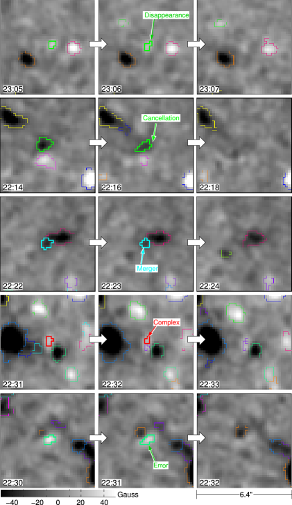
Figure 1.— Examples of Hinode/SOT/NFI images of five death types studied in this paper. Features are highlighted by the bordering color. Top Row: Disappearance, where a feature dies with no other features within 5 pixels; Second Row: Cancellation, where a feature dies near another of opposite polarity while approximately conserving flux; Third Row: Merger, where a feature dies near another of the same polarity while approximately conserving flux; Fourth Row: Complex, which involves multiple features where one satisfies the Cancellation criteria and another satisfies Merger; Bottom Row: Error, where a Cancellation would have been identified but the flux of the opposite-polarity feature increased instead of decreased. Each image shows a $6.4^{\prime\prime}\times 6.4^{\prime\prime}$ area on the photosphere and with the gray scale saturating at $\pm 50~{}\textrm{G}$.

3. Results

3.1. Summary of Detected Birth & Death Events

We identified 18297 features during the selected time period. There were 2088 features identified at the beginning of the dataset (birth Survival) and 2729 features identified at the end of the dataset (death Survival). There were 175 features that lived through the entire dataset and thus were classified as both birth Survival and death Survival.

Table LABEL:tab:N-stats shows the percentage (of the total number of features) for each birth / death type combination. Note that the 4 combinations of Fragmentation, birth Error, death Error, and Merger account for 60% of all features. We speculate that most of the birth Error and death Error events are simply fragmentations & mergers for which flux was not conserved in our simple two-feature interaction model.

Figure 2 shows the distribution of death type as a histogram, and also the flux removed according to death type. We accounted for flux by considering each feature to contain the maximum flux achieved in any single frame throughout its lifetime. The Disappearance, Cancellation and Complex event types are shaded in Figure 2. For the Error events, we estimate their contribution to the Cancellation and Merger classes by distributing them in the same proportion to that of the flux proportion of the Cancellation and Merger events. The vast majority of this proportion is from the Merger class and thus results in no flux removed. The additional contribution to the Cancellation events due to this is shown as the dashed extension. We disregard the Survival, Merger, and the remainder of the Error death events for the following reasons:

• Survival: These features survive beyond the time frame of the dataset and therefore do not remove flux during the study;

• Merger: These features remove no flux from the system since they lose their identity but not their flux by being absorbed into a like-polarity feature;

• Error: In their SWAMIS-detected form, these are not physical events but either Cancellation or Merger events, although we lack sufficient information to identify which.

Table 1Feature event history table: for each combination of birth & death type, the percentage of all 18297 features that were born and died in that combination.

Birth \ Death Type	Disappearance	Cancellation	Merger	Complex	Error	Survival	Total
Appearance	5.54%	0.21%	1.71%	0.01%	2.10%	1.77%	11.3%
Emergence	0.14%	0.15%	0.16%	0.04%	0.33%	0.13%	1.0 %
Fragmentation	1.42%	0.27%	20.6%	0.07%	12.7%	5.04%	40.1%
Complex	0.00%	0.01%	0.03%	0.01%	0.07%	0.02%	0.1 %
Error	1.52%	0.37%	13.6%	0.08%	13.5%	7.01%	36.1%
Survival	1.37%	0.21%	4.89%	0.03%	3.95%	0.96%	11.4%
Total	10.0%	1.2%	41.0%	0.23%	32.6%	14.9%	N=18297

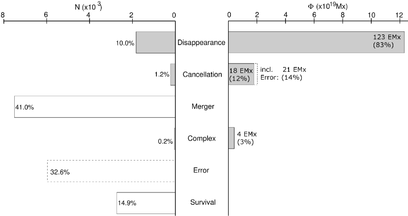
Figure 2.— Left: Histogram showing the number distribution of death type for the 18297 features detected using SWAMIS (i.e., bottom row in Table LABEL:tab:N-stats). The gray shading shows those three event types that remove flux from the photosphere: Disappearance, Cancellation, and Complex. Right: Histogram showing the flux ($\Phi$) removed by each of the death processes. See § 3.1 text.

3.2. Disappearance Events

As shown in Figure 2, Disappearances are responsible for the removal of the vast majority (83%) of the flux in the features identified by SWAMIS. We now investigate the means by which those features that died by Disappearance (bold font in Table LABEL:tab:N-stats) were born. Figure 3 shows the distribution by (left) number and (right) maximum flux of the birth process of each of the 1828 features that died by Disappearance. None of the 42 features with Complex births died by Disappearance, and we do not consider the Survival and Fragmentation events for reasons given above. The Error events have been distributed amongst the Emergence and Fragmentation events in the same way as was done for the Cancellation and Merger events before.

By far the most common birth process, in both number and flux, for the Disappearance events is Appearance. Following the results in SMT-2 and SMT-3 these are features that were born by the coalescence or convergence of smaller (many smaller than the spatial resolution of NFI) concentrations into a larger, more magnetically concentrated feature, and died by a break-up of the larger feature back into smaller concentrations.

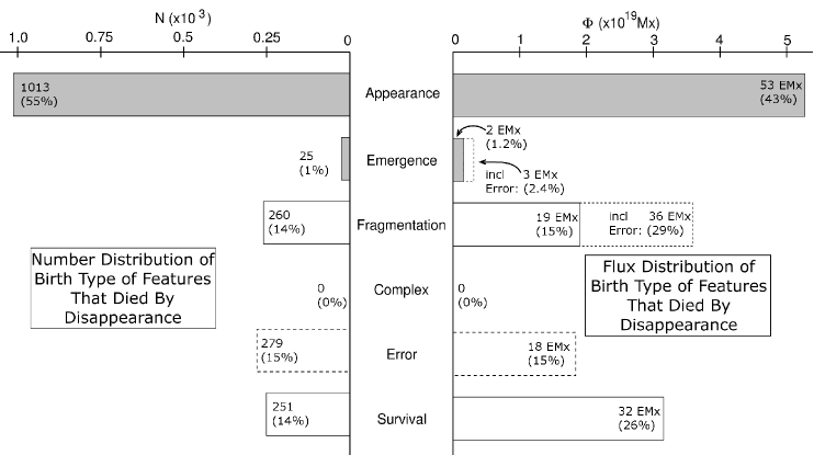
Figure 3.— Histograms showing the (left) number and (right) flux distributions of birth type for the 1828 features that died by Disappearance. These are in the same format as Figure 2 except the categories are by birth instead of death. The flux from the Error birth types have been distributed across the Emergence and Fragmentation events as was done for the Cancellation and Merger events in Figure 2, and is again shown by the dashed extensions to those two bars.

3.3. Disappearing Features that were Not Born by Appearance

It is not surprising that most features that died by Disappearance were also born by Appearance: in that case, the spatial distribution of the magnetic field in a relatively weakly-magnetized region changes such that a new feature is detected, then changes again such that the feature is no longer detected. However, many features that died by Disappearance (36% by number) were born by other event types. This is more surprising because a feature must be born in a more strongly magnetized region, move away from other features, and then Disappear. None of the Complex-born features and only 1.4% of the Emergence-born features died by Disappearance. Roughly the same proportion ($\sim$14%) of the Error-, Survival- and Fragmentation-born features died by Disappearance. Figure 4 shows examples of features that were born by Emergence (left column), Fragmentation (middle column), and Error (right column). Notice that in each case, the feature is born adjacent to other features, moves away from them, and then dies by Disappearance. This was typical of these types of events, and reinforces the idea that Disappearance is merely an extension, to unobservably small scales, of the shredding process that causes Fragmentation.

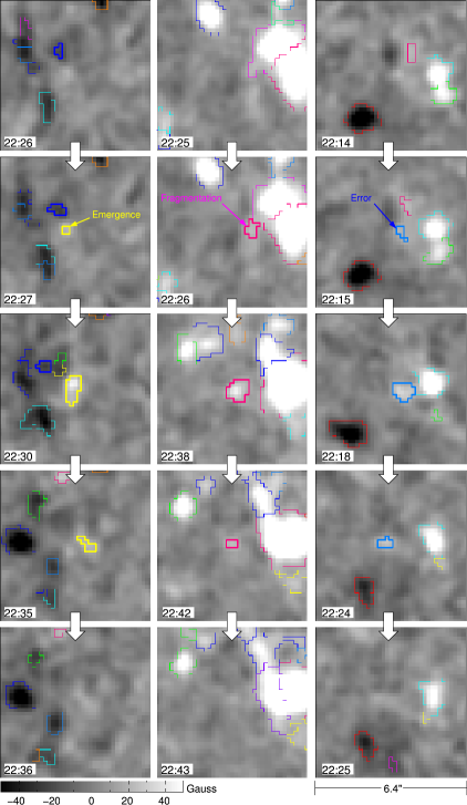
Figure 4.— Hinode/SOT/NFI images of three examples of features that died by Disappearance but were born by events other than Appearance. The birth events, indicated with the heavy colored boundaries, are Left: Emergence; Middle: Fragmentation; Right: Error. The $6.4^{\prime\prime}\times 6.4^{\prime\prime}$ spatial scale and the $\pm 50~{}\textrm{G}$ gray scale are the same as in Figure 1. Times in UT are at the bottom left of each image.

We interpret this result as a macrocosm of the dissipation process described in SMT-2 & SMT-3. These smaller fragments break away from a larger group, migrate away, and eventually themselves disappear. It seems likely that this process is due to further dissipation of the isolated feature in the reverse manner as those that are born by Appearance.

3.4. Temporal Ensemble Imaging

In order to test the idea that Disappearance events are typically due to the dispersal of magnetic flux, rather than unresolved cancellation, we produced ensemble images of 660 Disappearance events co-located in space and time. This technique, Event-Selected Ensemble Imaging (ESEI), is described in SMT-2 & SMT-3. It allows us to discriminate between Disappearances as asymmetric cancellations between a strong, localized flux concentration and a larger, undetectably weak opposing region, versus dispersals of existing flux. We find no evidence of significant amounts of opposite-polarity flux in the neighborhood of these Disappearances, similar to our previous analysis of Appearances.

To ensure that we fully understood the ensemble images themselves we produced an event-selected ensemble movie showing how the ensemble varied in the time steps surrounding the features’ deaths. For each Disappearance, we extracted a subimage of the magnetogram image in the time range $t_{death}-5...t_{death}+10$ minutes relative to the time of Disappearance. The center of the field-of-view of each subimage was initially taken to be the location of the center of flux of the Disappearing feature in the last frame the feature was visible. We call this method of producing the ensemble a “direct ensemble”. For the time of death and the 10 minutes afterwards, this is the best that can be reliably done. But for the times up to 5 minutes before the death, it can lead to unexpected results. Specifically, since the feature locations are moving through $x-y-t$ space in our dataset, in the ensemble image Disappearances seem to be increasing in strength during the 5 minutes leading up to the feature death, evidenced by an increasing peak and a smaller FWHM, a counter-intuitive result. This concentration over time is due to the uncorrelated (and uncorrected) motions of all the individual features in the ensemble.

Next, we formed a “motion-corrected ensemble” by choosing the center of the field of view of each subimage to coincide with the measured center of flux of each feature in the pre-death images. This eliminated the apparent concentration of the ensemble leading up to the death event, better approximating a typical feature’s behavior. The peak of the motion-corrected ensemble greatly exceeds the lower detection threshold (18 G) in the minutes before the death, slightly exceeds that threshold at the moment of death, and quickly drops below the threshold after the death.

Since the location of the feature’s center of flux is not measured after the feature has died, and kinematic estimates are unreliable, it is impossible to apply this same technique to the time after the feature death has occurred. However, by examining the difference between the two cases for the time before the death, we can estimate how much of the post-death spreading of the ensemble is due to translational motion of the newly-undetected flux, and how much is due to true dispersal of the flux.

In the 5 minutes prior to death, the FWHM of the direct ensemble decreases approximately linearly from 7.6 pixels at $t_{death}-5$ minutes to 4.6 pixels at $t_{death}$ (Figure 5). The FWHM of the motion-corrected ensemble is smaller, and decreases from 5.25 pixels to 4.6 pixels at $t_{death}$. By definition, the ensembles are the same at $t_{death}$. The difference between the two FWHMs is roughly linear in time over the range $t_{death}-4\leq t\leq t_{death}-1$ and has a slope of 0.44 pixels per frame, or about $0.85\textrm{ km s}^{-1}$.

Figure 5.— Time evolution of the ensemble FWHM for the cases of a direct ensemble (solid line) and a motion-corrected ensemble (dashed line), determined by fitting a Gaussian to the core of the ensemble. After $t_{death}+3$ min the fit becomes unreliable and is not shown.

After $t_{death}$ only the uncorrected FWHM is available. We do not attempt to extrapolate the motion of the feature in the few frames post-death, since this is unreliable: feature motion in adjacent frames is not correlated. The uncorrected FWHM increases from the minimum at $t_{death}$ approximately linearly with time, though the slope is 50–75% greater than the pre-death uncorrected slope.

The behavior of the motion-corrected ensemble FWHM is not consistent with any kind of diffusion of the ensemble magnetic field distribution. In the case of normal or anomalous diffusion, the FWHM would increase proportionally to some (positive) power of the elapsed time (Abramenko et al., 2011), whereas in our case the FWHM decreases with time. In order to understand this, we note that 1) only in the ensemble average of Disappearance events (and not in the individual events themselves) is the magnetic field roughly Gaussian-distributed on the surface; 2) the ensemble FWHM is not the same as the mean of the individual squared displacements; 3) the field being concentrated in intergranular lanes means that any diffusion would not be fully two-dimensional; 4) our motion-correction is based on the flux-weighted centroid of only those pixels above the low detection threshold (18 G); 5) the formation of a (meso-)granule around the time of $t_{death}$ would cause the proper motion of the features to increase in the minutes after $t_{death}$, and could result in the increase of the uncorrected FWHM slope at positive times in Fig. 5.

Finally, we note an unanticipated behavior of the Disappearance ensemble images, which is that the flux that can be confidently assigned to the Disappearing features (and not to the background) is not conserved either before or after $t_{death}$. This is not a by-product of the process that produces the ensemble, since the flux in individual Disappearance events also cannot be fully accounted for. Recognizing that our detection thresholds may be high, we produced images of some Disappearance events with a stretched-out gray scale and manually enclosed what we believed to be the largest possible extent of the Disappearing feature. Regardless, the total enclosed flux always decreased (by 30–50%) in the minutes after the feature’s death.

We consider likely explanations for this behavior to include 1) dispersal of the feature’s flux via horizontal advection of the field lines on very small scales, in a process that is completely analogous to the Fragmentation/Disappearance example in Figure 4; 2) non-linearity in the magnetograph detector, so that a decrease in the average line-of-sight field in the area of the photosphere subtended by a pixel does not result in a proportional decrease in the reported V/I signal and the observed magnetic field strength—such an effect is expected with the single line-wing magnetograms produced by NFI, and could account for the loss.

3.5. Feature Lifetimes & Partial Lifetimes

Figure 6 shows the distribution of feature lifetimes for those features that both were born and died during the observation. The line of best fit for lifetimes $\geq 4$ min on the log-log plot has a slope of -2.6. The mean (first moment) of a power-law distribution is finite for slopes $<-2$, and in this case the best-fit mean time is 10.7 min. It is clear that the lifetime distribution is not exponential, a point to which we return in § 4.2.

Since the total feature death rate is the sum of the rates of death by all causes, its mathematical reciprocal – the feature lifetime – is the harmonic sum of the “partial lifetimes” formed by taking the reciprocals of the various death processes. The total death rate by Cancellation in our observed patch of Sun was $3.5\times 10^{19}\textrm{ Mx h}^{-1}$. Dividing by the time-averaged total observed unsigned flux of $7.8\times 10^{20}\textrm{ Mx}$ yields a normalized Cancellation rate of $0.045~{}\textrm{h}^{-1}$, or a partial lifetime via Cancellation of $22~{}\textrm{h}$. This is $\approx 3$ times longer than the total lifetime of 8 h estimated for solar minimum by Hagenaar et al. (2003) based on MDI data, which included all types of feature death—even Disappearance. The larger lifetime is especially surprising considering the general trend toward shorter turnover times as resolution increases, and the lower resolution of MDI data compared to Hinode. This slower turnover rate omits consideration of cancellation at smaller scales, which will be considered in more detail in a subsequent paper. We discuss the implications of this $22~{}\textrm{h}$ partial lifetime due to Cancellation at the end of § 4.

Figure 6.— Distribution of feature lifetimes on a log-log plot, for only those features whose entire lifetime is observed in the dataset. The best-fit straight line has a slope $=-2.6$ for lifetimes $\geq 4$ min. The lower cutoff was chosen because a minimum feature lifetime of 4 frames was chosen in the tracking (§ 2.1); some features have a lifetime smaller than this cutoff because we do not filter features that are immediately adjacent to other features. The linear fit on a log-log plot suggests a power-law lifetime distribution, in contrast with the exponential lifetime distribution found by Zhou et al. (2010) using the same NFI data. See § 4.2 for more discussion.

3.6. Summary of Main Results

We summarize our main results here, and discuss their implications in the next section:

1. Disappearance events account for 10% of the observed feature deaths in our dataset but 83% of the flux lost to detection (§ 3.2), although the primary mechanism for Disappearance does not eliminate flux from the Sun;

2. Of those Disappearances, more than 50% were born by Appearance, suggesting a large amount of flux constantly being moved into and out of our range of detectability (§ 3.2);

3. We find no evidence that the Disappearance events are largely due to undetected cancellation, which agrees with our previous work on Appearances (§ 3.4);

4. The FWHM of the motion-corrected ensemble of Appearances decreases with time up to the moment of death, suggesting that normal planar diffusion is not an adequate description of this type of death event (§ 3.4);

5. The partial feature lifetime attributed to those features that died by Cancellation is 22 h, a factor of 3 slower than previously published quiet-Sun turnover times of 8 h (§ 3.5).

4. Discussion

4.1. The Reality of the Disappearance Events

A skeptical reader may wonder whether the fact that over half of the Disappearing features were born by Appearance suggests that these features could be more confidently attributed to a noise source and not to physical evolution of the magnetic field. Photon noise could hide an opposing pole around the Disappearing features, but as in SMT-2 and SMT-3 the ensemble imaging (§ 3.4) directly addresses that for all reasonable values of the magnetic pole asymmetry. Other sources of noise have been mitigated in the data preprocessing and tracking parameter selection. These noise sources could include, for example, a temporary and spatially isolated change in the magnetogram noise level (since the tracking code’s detection threshold values do not change over the course of the dataset), a change in the solar vertical velocity (since imaging magnetographs are sensitive to surface velocity fluctuations) or some other cause. Any or all of these could result in a small locus of pixels exceeding the detection threshold for a short period of time. Such an occurrence would result in the Appearance and subsequent Disappearance of a large number of features.

Our data preprocessing, feature filtering criteria, and event selection criteria were carefully chosen to take the above noise sources into account. For example, the FFT motion filter used in preprocessing was finely tuned to reduce noise and reject p-modes. The minimum feature lifetime was chosen to further reduce the effect of any photospheric line-of-sight velocity signal leaking into the magnetogram resulting in spurious feature detection.

Additionally, in post-processing we find no evidence that the Appearing-Disappearing features are anything other than real. First, and probably most important, a visual inspection of a movie showing the time and location of Appearances & Disappearances reveals no spatio-temporal clusters of these events. Second, the lifetime distribution of Appearance events is approximately the same as for other birth types (SMT-2), and in the present work 18% of the Appearing/Disappearing features have lifetimes $\geq$ 10 min, twice the period of p-modes which would be the most likely source of such a surface velocity change. Third, we would have likely seen a similar effect in the MDI Appearances work of SMT-2 but did not, and later confirmed using NFI that the MDI Appearances were real, thereby validating the SMT-2 work and the identical technique used in the present paper. Therefore we believe there is sufficient evidence that the Appearing-Disappearing features seen in this work also can be confidently attributed to true physical evolution of the photospheric magnetic field.

4.2. Feature History & Lifetimes

Other aspects of the feature history and lifetimes bear mentioning. First, we note that none of the features that died by Disappearance were of the Complex birth type. This is understandable when considering the definition of a Complex birth: there must be at least two nearby features, a like-polarity feature that satisfies the Fragmentation criterion and an opposite-polarity feature that satisfies the Emergence criterion. In order for a feature to be born in such a way, the local surface density of features must be relatively high. Since features do not migrate much over the course of their lifetime, the chance of such a feature dying in the complete absence of other features is very small.

The same logic applies to the fact that few of the features that die by Disappearance were born by Emergence, though since there is only one requirement for an Emergence birth, there are more Emergences than Complexes, and so by chance some of the features in our dataset have managed to migrate sufficiently away from their associated birth feature.

Finally, we note that the Hinode/SOT/NFI dataset used here is the same as that used in SMT-3, and is also the same as one of the two hour-long NFI datasets used in the by-eye analysis of Zhou et al. (2010). By comparing the bottom row of our Table LABEL:tab:N-stats or the left panel of Figure 2 to the bottom half of their Table 1, it is immediately obvious that their distribution of death events by type does not agree with our results. For example, fully ⅔ of their deaths were Disappearances (they used the label F${}_{\textrm{situ}}$), compared to only 10% of our feature deaths, and 11% of their deaths were cancellation, compared to only 1% of ours. We attribute this discrepancy to two factors. First, the event definitions used by us and them are not exactly the same. For example, we have no equivalent to their F${}_{\textrm{frag}}$ because we do not consider a feature to have died just because another feature was born by Fragmenting off a small portion of it, whereas they consider this to be the death of one feature and the birth of two different features. They have no equivalent to our Error or Complex, which may be due to the ability of the human brain to categorize complicated edge cases, and to our attempt to enforce physical flux conservation on events when possible. Second, they masked out stronger network concentrations and focused solely on the internetwork magnetic features, whereas we included all detected features in our feature tracking. The larger network concentrations exhibit much internal reorganization which results in many more Merger death events (their F${}_{\textrm{coal}}$) than they observe with the internetwork features. Assuming for a moment that all of our Mergers and death Error events are in network concentrations while all other events are in internetwork areas, 38% of the remainder of our deaths are Disappearances, which is closer to their result of 66.6%. Their masking out of network concentrations is also likely a main reason why their lifetime distribution does not agree with ours. They show (in their Figure 4) a lifetime distribution that is exponential, whereas our feature lifetime distribution is clearly not an exponential, but is closer to a power-law (Figure 6). We have previously shown (SMT-1) that the feature lifetime distribution is extremely difficult to reconcile between different algorithms (human or automated) even when operating on the same data with the intent of reproducing other algorithm’s results. We again emphasize that extreme caution must be employed when drawing scientific conclusions based on the distribution of magnetic feature lifetimes.

4.3. Concluding Remarks

Our results are consistent with the picture that arises from recent work by Parnell et al. (2009), who found that the number of magnetic features at a given flux scale follows a power law (and therefore has a scale-invariant distribution) over all observable scales. At any particular spatial resolution, the photospheric field is primarily contained in unobservably small packets of flux that migrate around the photosphere. Coalescence and shredding of these small packets are the dominant processes by which the observed visual magnetic features are created and destroyed. Far less flux submerges or emerges through the photosphere on observable scales than moves up or down the range of available scales, crossing the threshold of observability with any particular magnetograph.

This constant movement of magnetic flux up and down a range of spatial scales, into and out of the range of detectability of an instrument and/or detection algorithm, affects estimates of the “turnover time” of photospheric flux, which drives many coronal heating models. Estimates from feature creation rates (e.g., the 8–19 hr reported by Hagenaar et al., 2003) are not necessarily indicative of flux turnover because of the difference between feature birth and flux emergence (SMT-2); and feature average lifetimes are strongly dependent on the tracking algorithm (SMT-1). Depending on the tracking algorithm and the resulting lifetime distribution, the feature average lifetime may even be undefined (for a power-law distribution with a slope $\geq-2$).

We have introduced the concept of the partial feature lifetime, whereby the lifetime due to a particular feature death event type can be separated from the lifetime distribution as a whole. Traditional estimates of the flux turnover time are most closely related to the partial lifetime due to Cancellation, since flux must be introduced and removed from the photosphere in order for it to “turn over”. Our partial lifetime due to Cancellation (22 h) is $\approx 3$ times slower than previous estimates of the flux turnover time, which suggests that the shredding and dispersal of flux down to currently unobservable scales may be more important for determining the lifetime of magnetic features, than are the more familiar emergence and cancellation of flux. The true flux turnover time will depend strongly on how much magnetic flux is threading the photosphere at scales currently unobservable to imaging magnetographs, as well as the manner in which the flux evolves.

The result that most removal of visible flux occurs by shredding it to smaller scales may make nanoflare heating models simpler to sustain, both by enabling faster reconnection rates via the small interaction scales and by supplying several times the visible flux at smaller scales. We speculate that there is nothing physically special about the spatial resolution available to Hinode and that the same scaling law found by Parnell et al. (2009) will proceed to the diffusion length scale in the photosphere.

References

- Abramenko et al. (2011) Abramenko, V. I., Carbone, V., Yurchyshyn, V., et al. 2011, ApJ, 743, 133
- Berger et al. (1998) Berger, T. E., Löfdahl, M. G., Shine, R. S., & Title, A. M., 1998, ApJ, 495, 973
- Cadavid et al. (1999) Cadavid, A. C., Lawrence, J. K., & Ruzmaikin, A. A. 1999, ApJ, 521, 844
- DeForest et al. (2007) DeForest, C. E., Hagenaar, H. J., Lamb, D. A., Parnell, C. E., & Welsch, B. T., 2007, ApJ, 666, 576
- De Rosa et al. (2009) De Rosa, M. L., Schrijver, C. J., Barnes, G., et al. 2009, ApJ, 696, 1780
- Hagenaar (2001) Hagenaar, H. J. 2001, ApJ, 555, 448
- Hagenaar & Cheung (2009) Hagenaar, H. J. & Cheung, M., 2009, ASP Conf. Ser. 415, 167
- Hagenaar et al. (2008) Hagenaar, H. J., De Rosa, M. L., & Schrijver, C. J., 2008, ApJ, 678, 541
- Hagenaar et al. (2003) Hagenaar, H. J., Schrijver, C. J., & Title, A. M. 2003, ApJ, 584, 1107
- Hagenaar et al. (1999) Hagenaar, H. J., Schrijver, C. J., Title, A. M., & Shine, R. A., 1999, ApJ, 511, 932
- Harvey & Harvey (1973) Harvey, K. L. & Harvey, J. W., 1973, Solar Phys., 28, 61
- Harvey (1993) Harvey, K. L. 1993, Ph.D. Thesis
- Hathaway et al. (1996) Hathaway, D. H., Gilman, P. A., Harvey, J. W., Hill, F., Howard, R. F., Jones, H. P., Kasher, J. C., Leibacher, J. W., Pintar, J. A., & Simon, G. W., 1996, Science, 5266, 1306
- Iida et al. (2012) Iida, Y., Hagenaar, H. J., & Yokoyama, T. 2012, ApJ, 752, 149
- Krivova & Solanki (2004) Krivova, N. A., & Solanki, S. K., 2004, Astron. Astrophys. 417, 1125
- Lamb et al. (2008) Lamb, D. A., DeForest, C. E., Hagenaar, H. J., Parnell, C. E., & Welsch, B. T., 2008, Astrophys. J., 674, 520
- Lamb et al. (2010) Lamb, D. A., DeForest, C. E., Hagenaar, H. J., Parnell, C. E., & Welsch, B. T., 2010, Astrophys. J., 720, 1405
- Leighton (1964) Leighton, R. B., 1964, ApJ, 140, 1547
- Longcope & Kankelborg (1999) Longcope, D. W., & Kankelborg, C. C., 1999, ApJ, 524, 483
- López Fuentes et al. (2006) López Fuentes, M. C., Klimchuk, J. A., & Démoulin, P. 2006, ApJ, 639, 459
- Muller et al. (2000) Muller, R., Dollfus, A., Montague, M., Moity, J., & Vigneau. J., 2000, Astron. Astrophys., 339, 373
- Kosugi et al. (2007) Kosugi, T., Matsuzaki, K., Sakao, T., et al. 2007, Sol. Phys., 243, 3
- Livi et al. (1985) Livi, S. H. B., Wang, J., & Martin, S. F. 1985, Australian Journal of Physics, 38, 855
- Parker (1988) Parker, E. N. 1988, ApJ, 330, 474
- Parnel & Jupp (2000) Parnell, C. E. & Jupp, P. E., 2000, ApJ529, 554
- Parnell (2001) Parnell, C. E., 2001, Solar Phys., 200, 23
- Parnell et al. (2009) Parnell, C. E., DeForest, C. E., Hagenaar, H. J., Johnston, B. A., Lamb, D. A., & Welsch, B. T. 2009, ApJ698, 75
- Pevtsov & Acton (2001) Pevtsov, A. A., & Acton, L. W., 2001, ApJ, 554, 416
- Pietarila Graham et al. (2009) Pietarila Graham, J., Danilovic, S., & Schüssler, M. 2009, ApJ, 693, 1728
- Priest et al. (1994) Priest, E. R., Parnell, C. E., & Martin, S. F., 1994, ApJ, 427, 459
- Scherrer et al. (1995) Scherrer, P. H., Bogart, R. S., Bush, R. I., et al. 1995, Sol. Phys., 162, 129
- Schrijver et al. (1997) Schrijver, C. J., Title, A. M., van Ballegooijen, A. A., Hagenaar, H. J., and Shine, R. A., 1997, ApJ487, 424
- Schrijver & Zwaan (2000) Schrijver, C. J., & Zwaan, C., 2000, Solar and Stellar Magnetic Activity, Cambridge Uni. Press
- Simon et al. (1995) Simon, G. W., Title, A. M., & Weiss, N. O., 1995, ApJ, 442, 886
- Simon et al. (2001) Simon, G. W., Title, A. M., & Weiss, N. O., 2001, ApJ, 561, 427
- Smithson (1973) Smithson, R. C., 1973, Solar Phys., 29, 365
- Trujillo Bueno et al. (2004) Trujillo Bueno, J., Shchukina, N., & Asensio Ramos, A. 2004, Nature, 430, 326
- Tsuneta et al. (2008) Tsuneta, S. et al. 2008: Sol. Phys. 249, 167
- Wang et al. (1988) Wang, J., Shi, Z., Martin, S. F., & Livi, S. H. B., 1988, Vistas Astron., 31, 79
- Welsch et al. (2007) Welsch, B. T., Abbett, W. P., De Rosa, M. L., et al. 2007, ApJ, 670, 1434
- Welsch et al. (2013) Welsch, B. T., Fisher, G. H., & Sun, X. 2013, ApJ, 765, 98
- Zhou et al. (2010) Zhou, G. P., Wang, J. X., & Jin, C. L., 2010, Solar Phys., 267, 63