Quantum Monte Carlo calculation of the Fermi liquid parameters of the two-dimensional homogeneous electron gas

Abstract

Fermi liquid theory is the basic paradigm within which we understand the normal behavior of interacting electron systems, but quantitative values for the parameters that occur in this theory are currently unknown in many important cases. One such case is the two-dimensional homogeneous electron gas (2D HEG), which is realized in a wide variety of semiconductor devices. We have used quantum Monte Carlo (QMC) methods to calculate the Landau interaction functions between pairs of quasiparticles. We use these to study the Fermi liquid parameters, finding that finite-size effects represent a serious obstacle to the direct determination of Fermi liquid parameters in QMC calculations. We have used QMC data in the literature for other properties of the 2D HEG to assemble a set of “best available” values for the Fermi liquid parameters.

I Introduction

Many of the key theoretical developments in condensed matter physics have been concerned with the exploration of models that capture important aspects of the behavior of real materials. One of the most fundamental and useful model systems in the field is the homogeneous electron gas (HEG).giuliani The simplicity of the system (a gas of electrons moving in a uniform, neutralizing background) is deceptive: the model exhibits a rich range of physics and remains our basic starting point for understanding the behavior of charge carriers in metals and semiconductors.

The enormous theoretical challenge that must be overcome when trying to provide an accurate description of the HEG is that the electrons are strongly coupled by their mutual Coulomb repulsion. Nevertheless, many thermal and transport properties of the HEG can be described by ignoring electron-electron interactions altogether, resulting in the free-electron-gas model, in which each electron has its own well-defined energy and momentum. This observation, which predates quantum mechanics, was first explained within a general theoretical framework by Landau through the development of Fermi liquid theory.landau Although the existence of electron-electron repulsion and hence correlation dramatically changes the total energy of an electron gas, low-lying excitations have a nonvanishing overlap with the corresponding excitations of the noninteracting system, in which the single-particle orbitals are plane-wave momentum eigenstates. Hence we may associate each excited state of the interacting system with a particular set of quasiparticle momentum occupation numbers.

Remarkably, although Fermi liquid theory is our basic paradigm for the normal behavior of the fluid phase of an electron gas, quantitative values for the parameters that occur in this theory are essentially unknown. Armed with knowledge of the Fermi liquid parameters, we would have a complete parameterization of the low-energy excitations of the fully interacting electron gas. This would in turn allow nearly all thermodynamic, response, and transport properties to be determined quantitatively,giuliani enabling us to understand the precise role that correlation plays in the behavior of the HEG.

In this work we use quantum Monte Carlo (QMC) calculationsceperley_1980 ; foulkes_2001 to determine the Fermi liquid parameters of the two-dimensional (2D) HEG. Specifically, we have employed the variational Monte Carlo (VMC) and diffusion Monte Carlo (DMC) methods.foulkes_2001 VMC calculations involve taking the expectation value of a many-electron Hamiltonian with respect to a trial wave function that can be of arbitrary complexity. In our work, the trial wave function was optimized by minimizing first the variance of the energy,umrigar_1988a ; ndd_newopt then the energy expectation valueumrigar_emin with respect to wave-function parameters. In DMCceperley_1980 we simulate a process governed by the Schrödinger equation in imaginary time in order to project out the ground-state component of an initial wave function. We use the fixed-node approximationanderson_1976 to impose fermionic antisymmetry. All our QMC calculations were performed using the casino code.casino_ref

In Refs. ndd_band, and ndd_effmass2, we presented DMC calculations of the 2D HEG single-particle energy band ${\cal E}(k)$, enabling us to predict the quasiparticle effective mass $m^{\ast}$. In the present work we use DMC calculations to determine the Landau interaction functionsgiuliani and hence Fermi liquid parameters. Our approach is similar to that of the pioneering work of Kwon et al.,kwon_1994 which was undertaken eighteen years ago and is, to our knowledge, the only previous attempt to calculate the Fermi liquid parameters directly using QMC. Kwon et al. were unable to obtain consistent quantitative results, primarily because of the extremely small system sizes that they were forced to use at that time. However, there have been enormous developments in QMC methodology and computer power in the last two decades, and the time has come to revisit this grand-challenge problem. The major causes of computational expense in this work are (i) the need to overcome the finite-size errors in the Fermi liquid parameters by performing calculations at a range of system sizes and (ii) the fact that even for small numbers of electrons it is necessary to take the difference of very similar total energies to obtain the interaction functions. Point (ii) makes every aspect of this work computationally expensive: not only does each QMC calculation have to be sufficiently long that the statistical error bars are small compared with the differences to be resolved, but it must be ensured that the trial wave function is very highly optimized. These calculations were only made possible by access to the Jaguar machine at Oak Ridge Leadership Computing Facility.

The rest of this paper is structured as follows. In Sec. II we give an overview of the relevant aspects of Fermi liquid theory and describe our computational approach to the problem. Our results are presented in Sec. III. Finally, we draw our conclusions in Sec. IV. We use Hartree atomic units, in which the Dirac constant, the electronic charge and mass, and $4\pi$ times the permittivity of free space are unity ($\hbar=|e|=m_{e}=4\pi\epsilon_{0}=1$), throughout.

II Evaluating the Landau energy functional

II.1 Parameterization of excitation energies

The Landau energy functionalgiuliani is a parameterization of the energies of the ground state and low-lying excited states of the HEG:

$$E = E_{0}+\sum_{{\bf k},\sigma}{\cal E}_{\sigma}({\bf k})\delta{\cal N}_{{\bf k},\sigma}$$ (1)

$${}+\frac{1}{2}\sum_{({\bf k},\sigma)\neq({\bf k}^{\prime},\sigma^{\prime})}f_{\sigma,\sigma^{\prime}}({\bf k},{\bf k}^{\prime})\delta{\cal N}_{{\bf k},\sigma}\delta{\cal N}_{{\bf k}^{\prime},\sigma^{\prime}},$$

where $\delta{\cal N}_{{\bf k},\sigma}$ is the change to the ground-state quasiparticle occupation number for wavevector ${\bf k}$ and spin $\sigma$, and $E_{0}$ is the ground-state energy. Sufficiently close to the Fermi surface, the energy band ${\cal E}_{\sigma}({\bf k})$ is linear in $k$ and hence we may write

$${\cal E}_{\sigma}({\bf k})={\cal E}_{F}+\frac{k_{F}}{m^{\ast}}(k-k_{F}),$$ (2)

where ${\cal E}_{F}$ is the Fermi energy, $k_{F}$ is the Fermi wavevector, and $m^{\ast}$ is the quasiparticle effective mass. The Landau interaction function $f_{\sigma,\sigma^{\prime}}({\bf k},{\bf k}^{\prime})$ describes energy contributions arising from pairs of quasiparticles. Close to the Fermi surface we may neglect the dependence of $f$ on the magnitudes of the wavevectors and write the Landau interaction functions as $f_{\sigma\sigma^{\prime}}(\theta_{{\bf k}{\bf k}^{\prime}})$, where $\theta_{{\bf k}{\bf k}^{\prime}}$ is the angle between ${\bf k}$ and ${\bf k}^{\prime}$. The $l$th Fermi liquid parameter of the paramagnetic HEG is defined asgiuliani

$$F_{l}^{s,a}=\frac{AN^{\ast}_{p}(0)}{4\pi}\int_{0}^{2\pi}\left[f_{\uparrow\uparrow}(\theta_{{\bf kk}^{\prime}})\pm f_{\uparrow\downarrow}(\theta_{{\bf kk}^{\prime}})\right]\cos(l\theta)\,d\theta,$$ (3)

where $A=\pi r_{s}^{2}N$ is the area of the simulation cell, $r_{s}$ is the radius of the circle that contains one electron on average, $N$ is the number of electrons in the simulation cell, and $N^{\ast}_{p}(0)=m^{\ast}/\pi$ is the quasiparticle density of states per unit area at the Fermi surface. The suffixes $s$ and $a$ (for “symmetric” and “antisymmetric”) correspond to addition and subtraction in the integrand, respectively. For a fully ferromagnetic HEG, the $l$th Fermi liquid parameter is defined as

$$F_{l}=\frac{AN^{\ast}_{f}(0)}{2\pi}\int_{0}^{2\pi}f_{\uparrow\uparrow}(\theta_{{\bf kk}^{\prime}})\cos(l\theta)\,d\theta,$$ (4)

where the quasiparticle density of states per unit area is $N^{\ast}_{f}(0)=m^{\ast}/(2\pi)$.

II.2 Hartree-Fock theory

The total energy of a finite HEG in Hartree-Fock theory can be written as

$$E_{\rm HF}=\sum_{\sigma}\sum_{{\bf k}\in{\rm Occ}_{\sigma}}\frac{k^{2}}{2}-\frac{1}{2}\sum_{\sigma}\sum_{{\bf k}\neq{\bf k}^{\prime}\in{\rm Occ}_{\sigma}}\frac{2\pi}{A|{\bf k}-{\bf k}^{\prime}|}+\frac{Nv_{M}}{2},$$ (5)

where $v_{M}$ is the Madelung constant, $N$ is the number of electrons, $A$ is the area of the simulation cell and ${\rm Occ}_{\sigma}$ is the set of occupied states for spin $\sigma$. The Hartree-Fock energy is already in the form of the Landau energy functional and hence within Hartree-Fock theory the energy band is

$${\cal E}_{\sigma}({\bf k})=\frac{k^{2}}{2}-\sum_{{\bf k}^{\prime}\in{\rm GS}_{\sigma}}\frac{2\pi}{A|{\bf k}-{\bf k}^{\prime}|}$$ (6)

for ground-state unoccupied wavevectors, where ${\rm GS}_{\sigma}$ is the set of states occupied in the ground state, and

$${\cal E}_{\sigma}({\bf k})=\frac{k^{2}}{2}-\sum_{{\bf k}^{\prime}\neq{\bf k}\in{\rm GS}_{\sigma}}\frac{2\pi}{A|{\bf k}-{\bf k}^{\prime}|}$$ (7)

for ground-state occupied wavevectors. It also follows immediately from Eq. (5) that the Landau interaction functions in Hartree-Fock theory are

$$f_{\sigma\sigma}({\bf k},{\bf k}^{\prime})=-\frac{2\pi}{A|{\bf k}-{\bf k}^{\prime}|}\delta_{\sigma,\sigma^{\prime}}.$$ (8)

For excitations close to the Fermi surface, $|{\bf k}|\approx|{\bf k}^{\prime}|\approx k_{F}$, where $k_{F}$ is the Fermi wavevector. Let $\theta_{{\bf k}{\bf k}^{\prime}}$ be the angle between ${\bf k}$ and ${\bf k}^{\prime}$. Then $|{\bf k}-{\bf k}^{\prime}|^{2}=2k_{F}^{2}[1-\cos(\theta_{{\bf k}{\bf k}^{\prime}})]$. $A=\pi r_{s}^{2}N$ and, for a paramagnetic HEG, $k_{F}=\sqrt{2}/r_{s}$, so

$$Nf_{\sigma\sigma^{\prime}}({\bf k},{\bf k}^{\prime})=\frac{-\delta_{\sigma\sigma^{\prime}}}{r_{s}\sqrt{1-\cos(\theta_{{\bf k}{\bf k}^{\prime}})}}.$$ (9)

For a ferromagnetic HEG, $k_{F}=2/r_{s}$ and so

$$Nf_{\uparrow\uparrow}({\bf k},{\bf k}^{\prime})=\frac{-1}{r_{s}\sqrt{2-2\cos(\theta_{{\bf k}{\bf k}^{\prime}})}}.$$ (10)

II.3 QMC calculations

II.3.1 Evaluating the Landau interaction functions

By Eq. (1) we can evaluate the Landau interaction functions at a discrete set of angles $\{\theta_{i}\}$ as

$$f_{\sigma\sigma^{\prime}}(\theta_{i})=-[E_{\sigma\sigma^{\prime}}({\bf k}_{i},{\bf k}_{i}^{\prime})+E_{0}-E_{+}({\bf k}_{i})-E_{-}({\bf k}_{i}^{\prime})],$$ (11)

where $E_{0}$ is the ground-state energy, $E_{\sigma\sigma^{\prime}}({\bf k}_{i},{\bf k}_{i}^{\prime})$ is the total energy of an excited state in which an electron is promoted from ${\bf k}_{i}^{\prime}$ near the Fermi surface to ${\bf k}_{i}$ just above the Fermi surface, $\theta_{i}$ is the angle between ${\bf k}_{i}$ and ${\bf k}_{i}^{\prime}$, and $\sigma$ and $\sigma^{\prime}$ are the corresponding spins. $E_{+}({\bf k}_{i})$ and $E_{-}({\bf k}_{i}^{\prime})$ are the total energies of the system with an electron added to ${\bf k}_{i}$ and removed from ${\bf k}_{i}^{\prime}$, respectively.

II.3.2 Finite-size errors

Our QMC calculations were performed for electron gases in finite cells subject to periodic boundary conditions. The available wavevectors $\{{\bf k}\}$ are therefore the reciprocal lattice points of the simulation cell. The use of a finite cell prevents the description of long-range Coulomb and correlation effects,holzmann_2009 ; holzmann_2011 giving rise to finite-size errors in the Fermi liquid parameters. We have calculated the Landau interaction functions via total-energy differences in finite cells, used these to evaluate the Fermi liquid parameters, then extrapolated the parameters to the thermodynamic limit, where they should become independent of the choice of simulation cell and the precise excitations made to determine the interaction functions.

II.3.3 Simulation cell

In our calculations we have used square simulation cells with simulation-cell Bloch vectorrajagopal_1994 ; rajagopal_1995 ${\bf k}_{s}={\bf 0}$. There exist quantities such as the ground-state total energy, pair-correlation function, and static structure factor that can be twist averagedlin_twist_av in the conventional sense (i.e., one can evaluate estimators for these quantities at different simulation-cell Bloch vectors ${\bf k}_{s}$ and then average the results). However, there are other quantities such as the momentum density, the energy band, and the Landau interaction functions for which ${\bf k}_{s}$ determines the set of wavevectors at which the quantities are defined in a finite cell, so that by using different ${\bf k}_{s}$ we may obtain additional points on the quantity as a function of wavevector. The computational effort required to obtain excitation energies at different ${\bf k}_{s}$ is essentially the same as the computational effort required to obtain excitation energies by considering completely different excitations. Since the latter approach provides data that are in some sense more independent, we concluded that our computational effort was better invested in studying different excitations as opposed to changing ${\bf k}_{s}$.

The number of electrons in the ground state was chosen to be a “magic number,” corresponding to a closed-shell configuration in each case. For ferromagnetic HEGs, our calculations were performed with $N=29$, $57$, and $101$ electrons in the ground state. For paramagnetic HEGs our calculations were performed with $N=26$, $50$, $74$, and $114$ electrons in the ground state.

The simulation-cell area was held constant when electrons were added to or removed from the ground-state configuration. In the case of noninteracting electrons this gives the energy band ($k^{2}/2$) and Landau interaction functions (zero) exactly without finite-size error. (Note that in the free-electron model there are finite-size errors due to momentum quantization in the total energy, but no finite-size errors in the excitation energies.) For interacting electrons, the fact that the density changes when electrons are added or subtracted may be a source of finite-size error, but the error involved is certainly much smaller than the error that would result from allowing the cell area to change.

II.3.4 Trial wave function

We used trial wave functions of Slater-Jastrow-backflow form.ndd_jastrow ; kwon_bf ; backflow More detailed information about our trial wave functions can be found in Ref. ndd_effmass2, . In Ref. ndd_band, we argued that our DMC calculations for the 2D HEG retrieve more than 99% of the correlation energy.

The DMC time steps used in our calculations were $0.04$, $0.2$, and $0.4$ a.u. at $r_{s}=1$, 5, and 10, respectively, for paramagnetic HEGs, and $0.01$, $0.2$, and $0.4$ a.u. at $r_{s}=1$, 5, and 10, respectively, for ferromagnetic HEGs.

At $r_{s}=5$ we find the VMC energy variance per electron to be $1.48\times 10^{-4}$ and $2.44\times 10^{-5}$ a.u. for paramagnetic and ferromagnetic HEGs, respectively. Thus our trial wave functions are considerably more accurate for ferromagnetic HEGs, in which exchange effects are dominant. This suggests that it might be advantageous to use pairing (geminal) orbitals for opposite-spin electrons in paramagnetic HEGs.geminal Another possibility for improving the trial wave function would be to use different Jastrow factorsbouabca and backflow functions for each shell of plane-wave orbitals. However, given the expense of our calculations, there is at present little scope for using more sophisticated wave-function forms.

III Results

III.1 Landau interaction functions

The DMC Landau interaction functions at $r_{s}=1$, $5$, and $10$ are shown in Figs. 1, 2, and 3, respectively. The statistical error bars are very much smaller for ferromagnetic HEGs than for paramagnetic HEGs, reflecting the relative accuracy of the trial wave functions in the two cases (see Sec. II.3.4). Note that the data points are correlated, and so the error bars should be interpreted with caution. The Hartree-Fock interaction function (i.e., the exchange interaction: see Sec. II.2) is reasonably accurate at large $\theta$, but the parallel-spin interaction function is pathological as $\theta\rightarrow 0$ due to the lack of screening.

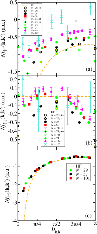
Figure 1: (Color online) Landau interaction functions $f_{\sigma\sigma^{\prime}}({\bf k},{\bf k}^{\prime})$ for 2D HEGs of density parameter $r_{s}=1$, multiplied by system size $N$. The parallel- and antiparallel-spin interaction functions in a paramagnetic HEG are shown in panels (a) and (b), respectively, while the interaction function in a fully ferromagnetic HEG is shown in panel (c). All results were obtained with a Slater-Jastrow-backflow trial wave function, except where labeled “SJ,” in which case a Slater-Jastrow wave function was used. The results labeled “++” were obtained in double-addition calculations, whereas those labeled “$--$” were obtained in double-subtraction calculations. All other results were obtained by promoting a single electron, leaving a hole. Note that the data points within each curve are correlated: for example, the interaction-function values at a given system size all depend on the DMC estimate of the ground-state energy. For comparison, we show the Hartree-Fock (HF) “interaction functions” for infinite system size [Eqs. (9) and (10)].

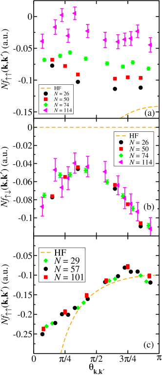
Figure 2: (Color online) As Fig. 1, but for HEGs at $r_{s}=5$.

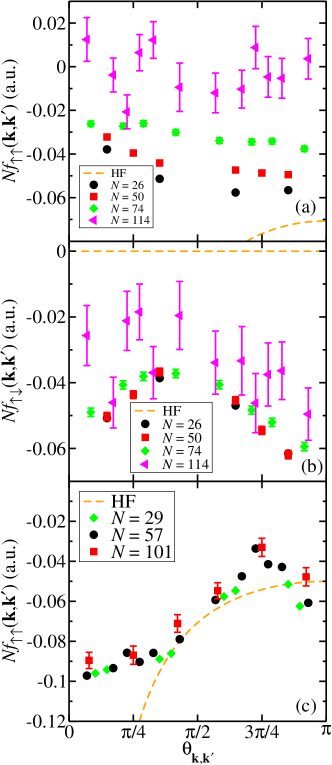
Figure 3: (Color online) As Fig. 1, but for HEGs at $r_{s}=10$.

The differences between the Slater-Jastrow and Slater-Jastrow-backflow DMC data are significant, confirming that the former are insufficiently accurate, as argued in Ref. kwon_1994, . There is a significant difference between the Landau interaction functions obtained from DMC calculations in which a single electron is promoted and calculations in which pairs of electrons are added or pairs of electrons are removed from the ground-state configuration. Finite-size effects in promotion energies are expected to be smaller because the density of the HEG in a finite cell is unchanged by such excitations, unlike double additions or subtractions. We have used only promotions in our production calculations to determine the Fermi liquid parameters.

III.2 Fermi liquid parameters

III.2.1 Numerical integration of the Landau interaction functions to find the Fermi liquid parameters

By Eq. (3), the Fermi liquid parameters divided by the effective mass $m^{\ast}$ for an $N$-electron paramagnetic HEG of density parameter $r_{s}$ can be written as

$$\frac{F_{l}^{s,a}}{m^{\ast}} = \frac{r_{s}^{2}N}{2\pi}\int_{0}^{\pi}\left[f_{\uparrow\uparrow}(\theta)\pm f_{\uparrow\downarrow}(\theta)\right]\cos(l\theta)\,d\theta$$ (12)

$$= \frac{r_{s}^{2}}{4}\left[a_{l}^{\uparrow\uparrow}\pm a_{l}^{\uparrow\downarrow}\right],$$

where

$$a_{l}^{\sigma\sigma^{\prime}}=\frac{2}{\pi}\int_{0}^{\pi}Nf_{\sigma\sigma^{\prime}}(\theta)\cos(l\theta)\,d\theta$$ (13)

is the $l$th Fourier component of $Nf_{\sigma\sigma^{\prime}}(\theta)$. To evaluate these Fourier components we use Simpson’s rule (integration of piecewise quadratic interpolants) generalized for the case of a nonuniform integration grid. The set of angles $\{\theta_{i}\}$ at which the integrand is available does not generally include the endpoints of the integration region ($0$ and $\pi$). Where necessary we integrate a straight-line interpolation of the closest two data points up to the endpoints of the integration region.

The Fourier coefficients $\{a_{l}^{\sigma\sigma^{\prime}}\}$ are linear in $E_{0}$, $E_{+}({\bf k}_{i})$, $E_{-}({\bf k}_{i}^{\prime})$, and $E_{\sigma\sigma^{\prime}}({\bf k}_{i},{\bf k}_{i}^{\prime})$. We therefore gather the coefficients of each of these in the expression for $a_{l}^{\sigma\sigma^{\prime}}$ [Eqs. (13) and (11)]. Finally, we evaluate the coefficients of $E_{0}$, $E_{+}({\bf k}_{i})$, $E_{-}({\bf k}_{i}^{\prime})$, and $E_{\sigma\sigma^{\prime}}({\bf k}_{i},{\bf k}_{i}^{\prime})$ in the expression for $F_{l}^{s,a}/m^{\ast}$ using Eq. (12). Since we have independent DMC estimates of $E_{0}$, $E_{+}({\bf k}_{i})$, $E_{-}({\bf k}_{i}^{\prime})$, and $E_{\sigma\sigma^{\prime}}({\bf k}_{i},{\bf k}_{i}^{\prime})$, we can evaluate both the expected Fermi liquid parameters divided by effective mass and the accompanying standard errors.

A systematic integration error arises from the use of numerical quadrature with a finite set of angles. This integration error is not included in our statistical error bars. We may place an upper bound on the error by comparing the Fermi liquid parameters obtained using (i) the generalized composite Simpson’s rule and (ii) the generalized composite trapezoidal rule to obtain $a_{l}^{\sigma\sigma^{\prime}}$. Results are given in Table 1 for HEGs at $r_{s}=5$. It is clear that the integration error is negligible compared with the random error for $F_{0}/m^{\ast}$ and $F_{1}/m^{\ast}$. For $F_{2}^{s,a}/m^{\ast}$ the effect of the choice of integration rule is more significant, especially for smaller numbers of electrons, where relatively few values of $\theta$ are available; however the error is still small compared with the overall results.

Table 1: Comparison of the first three Fermi liquid parameters (FLPs) in a.u. for a 74-electron paramagnetic HEG at $r_{s}=5$ ($F_{0}^{s}$, $F_{0}^{a}$, $F_{1}^{s}$, $F_{1}^{a}$, $F_{2}^{s}$, and $F_{2}^{a}$) and a 57-electron ferromagnetic HEG at $r_{s}=5$ ($F_{0}$, $F_{1}$, and $F_{2}$), derived from the Fourier components of the Slater-Jastrow-backflow DMC Landau interaction functions by numerical integration using the composite Simpson’s rule and the composite trapezoidal rule.

FLP over eff. mass	Simpson		Trapezoidal
$F_{0}^{s}/m^{\ast}$	$-1$.	$78(4)$	$-1$.	$78(4)$
$F_{0}^{a}/m^{\ast}$	$0$.	$01(1)$	$0$.	$01(1)$
$F_{1}^{s}/m^{\ast}$	$0$.	$18(1)$	$0$.	$18(1)$
$F_{1}^{a}/m^{\ast}$	$-0$.	$06(1)$	$-0$.	$06(1)$
$F_{2}^{s}/m^{\ast}$	$-0$.	$18(1)$	$-0$.	$22(1)$
$F_{2}^{a}/m^{\ast}$	$0$.	$12(1)$	$0$.	$12(1)$
$F_{0}/m^{\ast}$	$-1$.	$94(1)$	$-1$.	$94(1)$
$F_{1}/m^{\ast}$	$-0$.	$461(2)$	$-0$.	$466(3)$
$F_{2}/m^{\ast}$	$-0$.	$170(3)$	$-0$.	$193(3)$

The Fermi liquid parameters divided by the effective mass for a ferromagnetic HEG can be written as

$$\frac{F_{l}}{m^{\ast}}=\frac{r_{s}^{2}N}{2\pi}\int_{0}^{\pi}f_{\uparrow\uparrow}(\theta)\cos(l\theta)\,d\theta=\frac{r_{s}^{2}}{4}a_{l}^{\uparrow\uparrow}.$$ (14)

Hence we can evaluate the Fermi liquid parameters divided by the effective mass (with standard errors) for the ferromagnetic case using the same approach as for the paramagnetic case.

III.2.2 Finite-size extrapolation of the Fermi liquid parameters

We have calculated the Fermi liquid parameters divided by the effective mass at three or more system sizes for each density and magnetic state and we have extrapolated the parameters to infinite system size by assuming the finite-size error falls off as $N^{-1/4}$. This was the scaling found for Fermi liquid properties in Refs. holzmann_2009, and holzmann_2011, . The finite-size errors in the Fermi liquid parameters are determined by long-range correlation effects and we have therefore used the same system-size scaling for paramagnetic and ferromagnetic phases. The finite-size extrapolations at $r_{s}=1$, $5$, and $10$ are shown in Figs. 4, 5, and 6, respectively. The statistical error bars on the Fermi liquid parameters divided by the effective mass are generally much smaller than the apparent fluctuations as a function of system size. These fluctuations are presumably finite-size effects arising from the discrete nature of the lattice of wavevectors. We have therefore decided not to weight the residuals by the inverse of the error bars when performing the extrapolation to infinite system size. The quoted error bars on the extrapolated Fermi liquid parameters divided by the effective mass given in Tables 2 and 3 are obtained from an ordinary least-squares fit.

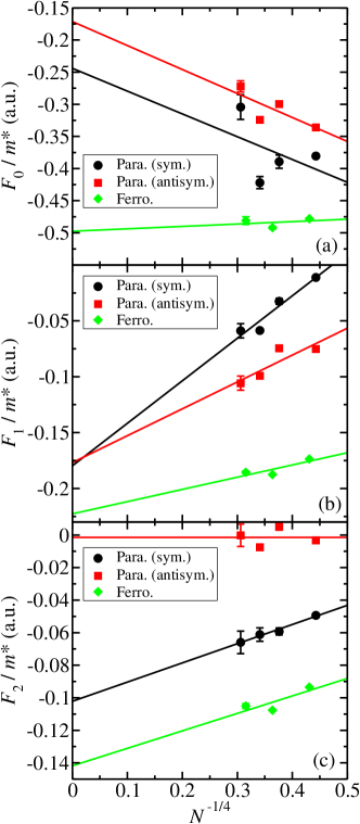
Figure 4: (Color online) Fermi liquid parameters divided by effective mass, (a) $F_{0}/m^{\ast}$, (b) $F_{1}/m^{\ast}$, and (c) $F_{2}/m^{\ast}$, against system size for paramagnetic HEGs (both symmetric and antisymmetric parameters) and ferromagnetic HEGs of density parameter $r_{s}=1$.

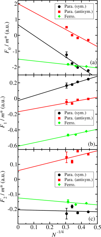
Figure 5: (Color online) As Fig. 4 but for HEGs of density parameter $r_{s}=5$.

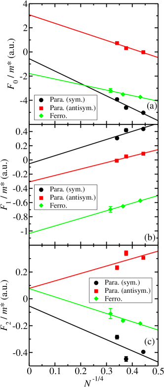
Figure 6: (Color online) As Fig. 4 but for HEGs of density parameter $r_{s}=10$.

There is no evidence for a systematic deviation of the Fermi liquid parameters from the fitted curves at small system sizes beyond the “noise” that obviously affects all the data points shown in Figs. 4, 5, and 6. We have therefore included all the data shown in these figures in our extrapolation to infinite system size.

We have attempted to check the exponent used for finite-size extrapolation of our Fermi liquid parameters by simultaneously fitting the functions

$$F_{i}(N)=c_{i}+a_{i}N^{\gamma}$$ (15)

to all our DMC data using a $\chi^{2}$ fit. The values of the parameters $c_{i}$ and $a_{i}$ differed for each Fermi liquid parameter at each density, while the exponent $\gamma$ was constrained to be the same in all cases. We find the optimal exponent to be $\gamma=-0.24(10)$, which is superficially consistent with the exponent $\gamma=-0.25$ determined theoretically by Holzmann et al.holzmann_2009 However, this is certainly not a conclusive numerical determination of the exponent $\gamma$. The $\chi^{2}$ value per data point with the optimal exponent of $\gamma=-0.24$ is $6.88$. The fact that this is much greater than 1 indicates that the fit is far from perfect. The main reason is the finite-size “noise” due to shell-filling effects, which is not included in the statistical error bars on the Fermi liquid parameters over effective mass. (The error bars only account for the random noise inherent in the QMC calculation.) If, instead of performing a $\chi^{2}$ fit, one performs a simple least-squares fit (i.e., each data point is weighted equally rather than by the squared reciprocal of the nominal error bar), one finds that the optimal exponent is $\gamma=-1(2)$. Alternatively, if one performs a $\chi^{2}$ fit with the exponent fixed at $\gamma=-1$, the resulting $\chi^{2}$ value is $7.26$ per data point, which is only slightly larger than the $\chi^{2}$ obtained with the “optimal” value of $\gamma=-0.24$.

In summary, we do not believe that we can meaningfully determine the finite-size scaling exponent $\gamma$ numerically, but our results are consistent with the value $\gamma=-0.25$ determined theoretically by Holzmann et al. We have therefore used this value in our analysis.

III.2.3 DMC results for the Fermi liquid parameters

Our results for the first three Fermi liquid parameters (symmetric and antisymmetric) of the paramagnetic HEG divided by the effective mass are given in Table 2, and the analogous results for a ferromagnetic HEG are given in Table 3.

Table 2: Fermi liquid parameters over effective mass in a.u. for the paramagnetic 2D HEG, extrapolated to the thermodynamic limit.

$r_{s}$	$F_{0}^{s}/m^{\ast}$		$F_{0}^{a}/m^{\ast}$		$F_{1}^{s}/m^{\ast}$		$F_{1}^{a}/m^{\ast}$		$F_{2}^{s}/m^{\ast}$		$F_{2}^{a}/m^{\ast}$
$1$	$-0$	$.2(2)$	$-0$	$.17(8)$	$-0$	$.18(3)$	$-0$	$.18(4)$	$-0$	$.102(5)$	$0$	$.00(2)$
$5$	$0$	$.7(8)$	$2$	$.0(7)$	$-0$	$.03(2)$	$-0$	$.17(7)$	$-0$	$.2(1)$	$0$	$.1(1)$
$10$	$-1$	$(1)$	$3$	$.1(7)$	$-0$	$.1(3)$	$-0$	$.3(1)$	$-0$	$.1(5)$	$0$	$.1(4)$

Table 3: Fermi liquid parameters over effective mass in a.u. for the ferromagnetic 2D HEG, extrapolated to the thermodynamic limit.

$r_{s}$	$F_{0}/m^{\ast}$		$F_{1}/m^{\ast}$		$F_{2}/m^{\ast}$
$1$	$-0$	$.50(4)$	$-0$	$.22(3)$	$-0$	$.14(3)$
$5$	$-1$	$.5(2)$	$-0$	$.61(6)$	$-0$	$.13(6)$
$10$	$-1$	$.8(3)$	$-1$	$.03(3)$	$0$	$.08(8)$

III.3 Relationships between the Fermi liquid parameters and other accessible quantities

III.3.1 Quasiparticle effective mass

By Eq. (2), the quasiparticle effective mass is

$$m^{\ast}=\frac{k_{F}}{(d{\cal E}/dk)_{k_{F}}}.$$ (16)

However, by Galilean invariance,giuliani the Fermi liquid parameter $F_{1}^{s}$ is related to the effective mass of the paramagnetic HEG via $m^{\ast}=1+F_{1}^{s}$, and, for the ferromagnetic HEG, $m^{\ast}=1+F_{1}$. Hence

$$m^{\ast}=\frac{1}{1-F_{1}^{s}/m^{\ast}},$$ (17)

for paramagnetic HEGs and

$$m^{\ast}=\frac{1}{1-F_{1}/m^{\ast}},$$ (18)

for ferromagnetic HEGs, so we can immediately evaluate the effective mass using the results in Tables 2 and 3.

In order to test the validity of our results, we compare the effective masses obtained using Eqs. (17) and (18) with the effective masses extracted directly from the energy bands (reported in Ref. ndd_effmass2, ) in Table 4. The two measures of the effective mass disagree by a statistically significant margin in half the cases. The enormous uncertainty in the finite-size extrapolation of the Fermi liquid parameters is the most likely reason for the disagreement. Direct calculation of the effective mass using a fit to the energy band together with Eq. (16) is likely to be more reliable, and we therefore suggest that the values of $F_{l}^{a,s}/m^{\ast}$ given in Tables 2 and 3 be multiplied by the effective mass $m^{\ast}$ reported in Ref. ndd_effmass2, to obtain the Fermi liquid parameters.

Table 4: Quasiparticle effective masses in a.u. for different density parameters $r_{s}$ and spin-polarization values $\zeta$, obtained directly from the energy bandndd_effmass2 and from the $F_{1}^{s}$ or $F_{1}$ Fermi liquid parameter [Eqs. (17) and (18)].

		Effective mass $m^{\ast}$
$r_{s}$	$\zeta$	Ref. ndd_effmass2,		Eqs. (17) and (18)
$1$	0	$0$.	$947(3)$	$0$.	$85(2)$
$5$	0	$0$.	$97(3)$	$0$.	$97(2)$
$10$	0	$0$.	$85(6)$	$0$.	$9(2)$
$1$	1	$0$.	$841(3)$	$0$.	$82(2)$
$5$	1	$0$.	$73(2)$	$0$.	$62(2)$
$10$	1	$0$.	$67(4)$	$0$.	$493(7)$

III.3.2 Isothermal compressibility

The isothermal compressibility $\kappa^{\ast}$ of the interacting 2D HEG at zero temperature satisfies

$$\frac{\kappa}{\kappa^{\ast}}=\frac{r_{s}^{4}}{4(1+\zeta^{2})}\left[\frac{\partial^{2}}{\partial r_{s}^{2}}-\frac{1}{r_{s}}\frac{\partial}{\partial r_{s}}\right]E(r_{s},\zeta),$$ (19)

where $E(r_{s},\zeta)$ is the total energy per electron as a function of density parameter $r_{s}$ and spin polarization $\zeta$, and $\kappa$ is the isothermal compressibility of the noninteracting system.giuliani

A parameterization of the correlation energy per electron in paramagnetic 2D electron gases is given in Ref. ndd_2dheg_expvals, , so that we may evaluate $\kappa/\kappa^{\ast}$ directly using Eq. (19). We refer to this as the total-energy approach.

Within Fermi liquid theory we havegiuliani

$$\frac{\kappa}{\kappa^{\ast}}=\frac{1}{m^{\ast}}+\frac{F_{0}^{s}}{m^{\ast}},$$ (20)

for a paramagnetic HEG and

$$\frac{\kappa}{\kappa^{\ast}}=\frac{1}{m^{\ast}}+\frac{F_{0}}{m^{\ast}},$$ (21)

for a ferromagnetic HEG, giving us a second approach for calculating the isothermal compressibility, which we refer to as the Fermi-liquid approach. The value of $F_{0}^{s}/m^{\ast}$ is taken from Table 2, while the value of $m^{\ast}$ is taken from Ref. ndd_effmass2, .

A comparison of the isothermal compressibilities obtained using these two different approaches is given in Table 5. Unfortunately the results are quite different. We verified that the compressibility ratios evaluated using the total-energy approach with two different parameterizations of the correlation energyndd_2dheg_expvals ; attaccalite_2002 agree to at least three significant figures. We therefore believe that the isothermal compressibilities obtained from fits to ground-state DMC energy calculations are reliable.

Table 5: Modification to the isothermal compressibility and spin susceptibility of a paramagnetic 2D HEG due to electron interactions as calculated (i) from Eqs. (19) and (22) together with parameterizations of the total energy per particlendd_2dheg_expvals ; attaccalite_2002 and (ii) from Eqs. (20) and (23) together with the present calculation of the Fermi liquid properties.

	Compress. ratio $\kappa/\kappa^{\ast}$				Spin-suscept. ratio $\chi/\chi^{\ast}$
$r_{s}$	Tot. en. ap.		Fermi liq. ap.		Tot. en. ap.		Fermi liq. ap.
1	$0$.	$533$	$0$.	$9(2)$	$0$.	$691$	$0$.	$89(8)$
5	$-1$.	$735$	$1$.	$7(8)$	$0$.	$296$	$3$.	$0(7)$
10	$-4$.	$989$	$0$.	$2(2)$	$0$.	$153$	$4$.	$3(7)$

The values of $F_{0}^{s}/m^{\ast}$ implied by the ground-state total-energy results of Ref. ndd_2dheg_expvals, together with the effective-mass data reported in Ref. ndd_effmass2, are $F_{0}^{s}/m^{\ast}=\kappa/\kappa^{\ast}-1/m^{\ast}=-0.523(2)$, $-2.77(2)$, and $-6.17(4)$ at $r_{s}=1$, $5$, and $10$, respectively. These are relatively close to the values of $F_{0}^{s}/m^{\ast}$ obtained at finite system sizes (see Figs. 4, 5, and 6).

The analogous results for a ferromagnetic HEG are shown in Table 6. Again we see a significant difference between the compressibilities obtained directly from the total energy and from the Fermi liquid parameters.

Table 6: Modification to the isothermal compressibility of a ferromagnetic 2D HEG due to electron interactions as calculated (i) from Eqs. (19) together with a parameterization of the total energy per particleattaccalite_2002 and (ii) from Eqs. (21) together with the present calculation of the Fermi liquid properties.

	Compress. ratio $\kappa/\kappa^{\ast}$
$r_{s}$	Tot. en. ap.		Fermi liq. ap.
1	$0$.	$680$	$0$.	$69(4)$
5	$-0$.	$636$	$-0$.	$1(2)$
10	$-2$.	$347$	$-0$.	$3(3)$

III.3.3 Isothermal spin susceptibility

The isothermal spin susceptibility $\chi^{\ast}$ of a paramagnetic HEG at zero temperature satisfiesgiuliani

$$\frac{\chi}{\chi^{\ast}}=r_{s}^{2}\left(\frac{\partial^{2}E}{\partial\zeta^{2}}\right)_{\zeta=0},$$ (22)

where $\chi$ is the (Pauli) spin susceptibility of a free electron gas. Attaccalite et al.attaccalite_2002  have reported a parameterization of the correlation energy obtained in QMC calculations as a function of both density parameter $r_{s}$ and spin polarization $\zeta$. Hence we can use Eq. (22) to evaluate $\chi/\chi^{\ast}$ using the total-energy approach.

Within Fermi liquid theory the isothermal spin susceptibility $\chi^{\ast}$ of an interacting electron system satisfiesgiuliani

$$\frac{\chi}{\chi^{\ast}}=\frac{1}{m^{\ast}}+\frac{F_{0}^{a}}{m^{\ast}}.$$ (23)

The value of $F_{0}^{a}/m^{\ast}$ is taken from Table 2, while the value of $m^{\ast}$ is taken from Ref. ndd_effmass2, .

We compare the isothermal spin susceptibilities obtained using these two approaches in Table 5. The results obtained from a fit to the ground-state energy as a function of density parameter and spin polarization are quite different to the results obtained using our Fermi liquid parameters.

The values of $F_{0}^{a}/m^{\ast}$ implied by the ground-state total-energy results of Ref. attaccalite_2002, together with the effective-mass data reported in Ref. ndd_effmass2, are $F_{0}^{a}/m^{\ast}=\chi/\chi^{\ast}-1/m^{\ast}=-0.365(2)$, $-0.73(2)$, and $-1.02(4)$ at $r_{s}=1$, $5$, and $10$, respectively. These are relatively close to the results obtained at finite system size shown in Figs. 4, 5, and 6. The finite-size extrapolation appears to move the Fermi liquid parameters away from the values suggested by the spin susceptibility.

Both the isothermal compressibility and spin susceptibility results show that we are not able to extrapolate the Fermi liquid parameters to the thermodynamic limit with quantitative accuracy. There is no clear numerical evidence to support the $N^{-1/4}$ scaling, and in most cases any systematic finite-size error appears to be swamped by oscillations due to shell-filling effects in the Fermi liquid parameters as a function of system size.

III.4 Summary of the “best available” Fermi liquid parameters

In Tables 7 and 8 we summarize the Fermi liquid parameters determined from QMC results reported in Refs. ndd_effmass2, ; ndd_2dheg_expvals, ; attaccalite_2002, . The values of $F_{1}^{s}$ and $F_{1}$ are determined using the effective masses reported in Ref. ndd_effmass2, , the values of $F_{0}^{s}$ are determined using the effective masses of Ref. ndd_effmass2, together with the parameterization of the correlation energy given in Ref. ndd_2dheg_expvals, , and the values of $F_{0}$ and $F_{0}^{a}$ are determined using the effective masses together with the parameterization of the correlation energy given in Ref. attaccalite_2002, .

Table 7: Best available Fermi liquid parameters of the paramagnetic 2D HEG as inferred from QMC results in the literature (see text).

$r_{s}$	$F_{0}^{s}$		$F_{0}^{a}$		$F_{1}^{s}$
$1$	$-0$	$.495(2)$	$-0$	$.346(2)$	$-0$	$.053(3)$
$5$	$-2$	$.68(5)$	$-0$	$.713(9)$	$-0$	$.03(3)$
$10$	$-5$	$.2(3)$	$-0$	$.870(9)$	$-0$	$.15(6)$

Table 8: Best available Fermi liquid parameters of the ferromagnetic 2D HEG as inferred from QMC results in the literature (see text).

$r_{s}$	$F_{0}$		$F_{1}$
$1$	$-0$	$.428(2)$	$-0$	$.159(3)$
$5$	$-1$	$.46(1)$	$-0$	$.27(2)$
$10$	$-2$	$.57(9)$	$-0$	$.33(4)$

IV Conclusions

We have used QMC methods to calculate the Fermi liquid parameters of the 2D HEG. However, the results we have obtained are inconsistent with more direct evaluations of the isothermal compressibility and spin susceptibility. Determining the Fermi liquid parameters therefore remains a grand-challenge problem due to the enormous difficulty in extrapolating the QMC data to the thermodynamic limit. Nevertheless, we have been able to describe the difficulties of determining the Fermi liquid parameters using QMC techniques, and we have assembled a set of “best available” values of some of the parameters. Our work demonstrates considerable progress in determining accurate values for the Fermi liquid parameters of the 2D HEG. Although the quasiparticle effective masses deduced from our determination of the Fermi liquid parameters are only in approximate agreement with the values obtained directly from the energy band,ndd_effmass2 neither method shows mass enhancement at low densities.

- (1) G. F. Giuliani and G. Vignale, Quantum Theory of the Electron Liquid, CUP, Cambridge (2005).
- (2) L. D. Landau, JETP 3, 920 (1957); L. D. Landau, JETP 5, 101 (1957); L. D. Landau, JETP 8, 70 (1959).
- (3) D. M. Ceperley and B. J. Alder, Phys. Rev. Lett. 45, 566 (1980).
- (4) W. M. C. Foulkes, L. Mitas, R. J. Needs, and G. Rajagopal, Rev. Mod. Phys. 73, 33 (2001).
- (5) C. J. Umrigar, K. G. Wilson, and J. W. Wilkins, Phys. Rev. Lett. 60, 1719 (1988).
- (6) N. D. Drummond and R. J. Needs, Phys. Rev. B 72, 085124 (2005).
- (7) C. J. Umrigar, J. Toulouse, C. Filippi, S. Sorella, and R. G. Hennig, Phys. Rev. Lett. 98, 110201 (2007).
- (8) J. B. Anderson, J. Chem. Phys. 65, 4121 (1976).
- (9) R. J. Needs, M. D. Towler, N. D. Drummond, and P. López Ríos, J. Phys.: Condens. Matter 22, 023201 (2010).
- (10) N. D. Drummond and R. J. Needs, Phys. Rev. B 80, 245104 (2009).
- (11) N. D. Drummond and R. J. Needs, Phys. Rev. B 87, 045131 (2013).
- (12) Y. Kwon, D. M. Ceperley, and R. M. Martin, Phys. Rev. B 50, 1684 (1994).
- (13) M. Holzmann, B. Bernu, V. Olevano, R. M. Martin, and D. M. Ceperley, Phys. Rev. B 79, 041308(R) (2009).
- (14) M. Holzmann, B. Bernu, and D. M. Ceperley, J. Phys.: Conf. Ser. 321, 012020 (2011).
- (15) G. Rajagopal, R. J. Needs, S. Kenny, W. M. C. Foulkes, and A. James, Phys. Rev. Lett. 73, 1959 (1994).
- (16) G. Rajagopal, R. J. Needs, A. James, S. D. Kenny, and W. M. C. Foulkes, Phys. Rev. B 51, 10591 (1995).
- (17) C. Lin, F. H. Zong, and D. M. Ceperley, Phys. Rev. E 64, 016702 (2001).
- (18) N. D. Drummond, M. D. Towler, and R. J. Needs, Phys. Rev. B 70, 235119 (2004).
- (19) Y. Kwon, D. M. Ceperley, and R. M. Martin, Phys. Rev. B 48, 12037 (1993).
- (20) P. López Ríos, A. Ma, N. D. Drummond, M. D. Towler, and R. J. Needs, Phys. Rev. E 74, 066701 (2006).
- (21) M. Casula and S. Sorella, J. Chem. Phys. 119, 6500 (2003).
- (22) T. Bouabça, B. Braïda, and M. Caffarel, J. Chem. Phys. 133, 044111 (2010).
- (23) N. D. Drummond and R. J. Needs, Phys. Rev. B 79, 085414 (2009).
- (24) C. Attaccalite, S. Moroni, P. Gori-Giorgi, and G. B. Bachelet, Phys. Rev. Lett. 88, 256601 (2002); C. Attaccalite, S. Moroni, P. Gori-Giorgi, and G. B. Bachelet, Phys. Rev. Lett. 91, 109902(E) (2003).