Information and treatment of unknown correlations
in the combination of measurements using the BLUE method

Abstract

We discuss the effect of large positive correlations in the combinations of several measurements of a single physical quantity using the Best Linear Unbiased Estimate (BLUE) method. We suggest a new approach for comparing the relative weights of the different measurements in their contributions to the combined knowledge about the unknown parameter, using the well-established concept of Fisher information. We argue, in particular, that one contribution to information comes from the collective interplay of the measurements through their correlations and that this contribution cannot be attributed to any of the individual measurements alone. We show that negative coefficients in the BLUE weighted average invariably indicate the presence of a regime of high correlations, where the effect of further increasing some of these correlations is that of reducing the error on the combined estimate. In these regimes, we stress that assuming fully correlated systematic uncertainties is not a truly conservative choice, and that the correlations provided as input to BLUE combinations need to be assessed with extreme care instead. In situations where the precise evaluation of these correlations is impractical, or even impossible, we provide tools to help experimental physicists perform more conservative combinations.

1 Introduction

Our knowledge about some of the most fundamental parameters of physics is derived from a vast number of measurements produced by different experiments using several complementary techniques. Many statistical methods are routinely used bib:pdg to combine the available data and extract the most appropriate estimates of the values and uncertainties for these parameters, properly taking into account all correlations between the measurements. One the most popular methods for performing these combinations is the Best Linear Unbiased Estimate (BLUE) technique, an approach first introduced in the 1930’s bib:aitken and whose reformulation in the context of high-energy physics bib:lyons ; bib:valassi has been routinely used for the combination of the precision measurements performed by experiments at the LEP bib:lep_ewwg , Tevatron bib:tev_top and LHC bib:lhc_top colliders, as well as in other domains.

To quantify the “relative importance” of each measurement in its contribution to the combined knowledge about the measured physical quantity, its coefficient in the BLUE weighted average is traditionally used. In many examples in the literature where the BLUE technique has been used, the combinations are dominated by systematic uncertainties, often assumed as fully correlated among different measurements. This often leads to situations where one or more measurements contribute with a negative BLUE coefficient, pushing experimentalists to redefine the “relative importance” of a measurement as the absolute value of its BLUE coefficient, normalised to the sum of the absolute values of all coefficients bib:tev_top ; bib:lhc_top . In our opinion, this approach is incorrect.

In this paper, we propose a different approach for comparing the relative contributions of the measurements to the combined knowledge about the unknown parameter, using the well-established concept of Fisher information bib:fisher . We also show that negative coefficients in the BLUE weighted average invariably indicate the presence of very high correlations, whose marginal effect is that of reducing the error on the combined estimate, rather than increasing it. In these regimes, we stress that taking systematic uncertainties to be fully (i.e. 100%) correlated is not a conservative assumption, and we therefore argue that the correlations provided as inputs to BLUE combinations need to be assessed with extreme care. In those situations where their precise evaluation is impossible, we offer a few guidelines and tools for critically re-evaluating these correlations, in order to help experimental physicists perform more “conservative” combinations. In our discussion, we will generally limit ourselves to BLUE combinations of a single measured parameter and where the correlations used as inputs to the combination are positive. Many of the concepts and tools we present could be applied also to the more general cases of BLUE combinations of several measured parameters, and/or involving also negative correlations between measurements, but this discussion is beyond the scope of this paper.

The outline of this article is the following. In Sec. 2 we review the definition of “relative importance” of a measurement in a BLUE combination as presented by some papers in the literature and we present our objections to it by using a simple numerical example. We then present our alternative definitions of information weights in Sec. 3, after a brief recall of the definition of Fisher information and of its relevant features. By studying marginal information and information derivatives, in Sec. 4 we show that negative BLUE coefficients in the combination of several measurements of one parameter are always a sign of a “high-correlation” regime, thus generalising the results presented for two measurements by the authors of Ref. bib:lyons . In Sec. 5 we go on to discuss practical guidelines and tools, illustrated by numerical examples, to identify correlations that may have been overestimated and to review them in a more “conservative” way. In Sec. 6 we summarize our discussion and present some concluding remarks.

2 “Relative importance” and negative BLUE coefficients

In the BLUE technique, the best linear unbiased estimate of each unknown parameter is built as a weighed average of all available measurements. The coefficients multiplying the measurements in each linear combination are determined as those that minimize its variance, under the constraint of a normalisation condition which ensures that this represents an unbiased estimate of the corresponding parameter. As discussed extensively in Refs. bib:lyons ; bib:valassi ; bib:bos , this technique is equivalent to minimizing the weighted sum of squared distances of the measurements from the combined estimates, using as weighting matrix the input covariance matrix of the measurements, which is assumed to be known a priori.

In the case of $n$ measurements $y_{i}$ of a single parameter whose true value is $Y$, in particular, the best linear unbiased estimate $\hat{Y}$ can be determined as follows. First, the BLUE should be a linear combination $\hat{Y}=\sum_{i=1}^{n}\,\lambda_{i}\,y_{i}$ of the available measurements. Second, the BLUE should be an unbiased estimator, i.e. its expectation value ${\mathbb{E}}[\hat{Y}]$ should be equal to the true value $Y$ of the unknown parameter. Assuming that each measurement is also an unbiased estimator, i.e. that its outcomes are distributed as random variables with expectation values ${\mathbb{E}}[y_{i}]=Y$, this is equivalent to requiring a normalisation condition $\sum_{i=1}^{n}\lambda_{i}=1$ for the coefficients $\lambda_{i}$ in the linear combination. Third, the BLUE should be the best of such unbiased linear combinations, i.e. that for which the combined variance $\sigma_{\raisebox{1.0pt}{\tiny$\hat{Y}$}}^{2}=\sum_{i=1}^{n}\sum_{j=1}^{n}\lambda_{i}\,\mathcal{M}_{ij}\,\lambda_{j}$, where $\mathcal{M}$ is the covariance matrix of the measurements, is minimized. It is then easy to show bib:lyons that $\hat{Y}$ is the best linear unbiased estimate if the coefficients $\lambda_{i}$ are equal to

$$\lambda_{i}=\frac{\raisebox{2.0pt}{$\bigl{(}\mathcal{M}^{-1}\mathbf{U}\bigr{)}_{i}$}}{\raisebox{-2.0pt}{$\tilde{\mathbf{U}}\mathcal{M}^{-1}\mathbf{U}$}},$$ (1)

where $\mathbf{U}$ is a vector whose elements are all equal to 1.

While the normalisation condition ensures that the coefficients $\lambda_{i}$ sum up to 1, one peculiar and somewhat counter-intuitive feature of this method is that some of these individual coefficients may be negative. Negative coefficients in the BLUE weighted averages apparently still pose a problem of interpretation sometimes, especially if these coefficients are used to compare the contributions of the different measurements to the combined knowledge about the measured observable. For instance, the “relative importance” of each measurement in the combination of ATLAS and CMS results on the top quark mass bib:lhc_top was defined as the absolute value of its coefficient in the BLUE weighted average, divided by the sum of the absolute values of the coefficients for all input measurements,

$$\mathrm{RI}_{i}=\frac{|\lambda_{i}|}{\sum_{j=1}^{n}|\lambda_{j}|}.$$ (2)

The same procedure had already been used to visualize the “weight that each measurement carries in the combination” of CDF and D0 results on the top quark mass bib:tev_top . In both cases, the relative importances of the $n$ measurements sum up to 1 by definition, $\sum_{i=1}^{n}\mathrm{RI}_{i}=1$.

In our opinion, this procedure is an artefact that is conceptually wrong and suffers from two important limitations: first, it is not internally self-consistent and may easily lead to numerical conclusions which go against common sense; second, it does not help to understand in which way the results with negative coefficients contribute to reducing the uncertainties on the combined estimates. We will use a simple example to illustrate the first objection. Consider the combination of two uncorrelated measurements $y_{\raisebox{-1.0pt}{\scriptsize A}}=103.00\pm 3.87$ and $y_{\raisebox{-1.0pt}{\scriptsize B}}=98.00\pm 3.16$ of an observable $Y$ in the appropriate units. The covariance matrix is then

$$\left(\begin{array}[]{c|c}\sigma_{\raisebox{-1.0pt}{\scriptsize A}}^{2}&0\\ \hline\cr 0&\sigma_{\raisebox{-1.0pt}{\scriptsize B}}^{2}\\ \end{array}\right)=\left(\begin{array}[]{c|c}15.00&0\\ \hline\cr 0&10.00\\ \end{array}\right)$$ (3)

and the BLUE for their combination is $\hat{Y}=\lambda_{\raisebox{-1.0pt}{\scriptsize A}}y_{\raisebox{-1.0pt}{\scriptsize A}}+\lambda_{\raisebox{-1.0pt}{\scriptsize B}}y_{\raisebox{-1.0pt}{\scriptsize B}}=100.00\pm 2.45$, where the coefficients of these two uncorrelated measurements in the BLUE weighted average, $\lambda_{\raisebox{-1.0pt}{\scriptsize A}}\!=\!0.4$ and $\lambda_{\raisebox{-1.0pt}{\scriptsize B}}\!=\!0.6$, are proportional to the inverses of the variances $\sigma_{\raisebox{-1.0pt}{\scriptsize A}}^{2}$ and $\sigma_{\raisebox{-1.0pt}{\scriptsize B}}^{2}$ as expected from simple error propagation. It is rather intuitive in this case to claim that the relative contributions to the knowledge about $Y$ contributed by the two independent measurements A and B can be quantified by their BLUE coefficients, 40% for A and 60% for B. As $\lambda_{\raisebox{-1.0pt}{\scriptsize A}}$ and $\lambda_{\raisebox{-1.0pt}{\scriptsize B}}$ are both positive, these are also the “relative importances” of A and B according to Eq. 2.

Imagine now that $y_{\raisebox{-1.0pt}{\scriptsize B}}$ is not the result of a direct measurement, but is itself the result of the combination of two measurements $y_{\raisebox{-1.0pt}{\scriptsize B1}}=99.00\pm 4.00$ and $y_{\raisebox{-1.0pt}{\scriptsize B2}}=101.00\pm 8.00$, where a high positive correlation $\rho=0.875$ between them leads to negative BLUE coefficients in their weighted average $y_{\raisebox{-1.0pt}{\scriptsize B}}=1.5\!\times\!y_{\raisebox{-1.0pt}{\scriptsize B1}}-0.5\!\times\!y_{\raisebox{-1.0pt}{\scriptsize B2}}=98.00\pm 3.16$. Instead of combining first $y_{\raisebox{-1.0pt}{\scriptsize B1}}$ and $y_{\raisebox{-1.0pt}{\scriptsize B2}}$ and then adding $y_{\raisebox{-1.0pt}{\scriptsize A}}$, one could also combine $y_{\raisebox{-1.0pt}{\scriptsize A}}$, $y_{\raisebox{-1.0pt}{\scriptsize B1}}$ and $y_{\raisebox{-1.0pt}{\scriptsize B2}}$ directly using the full covariance matrix

$$\left(\begin{array}[]{c|cc}\sigma_{\raisebox{-1.0pt}{\scriptsize A}}^{2}&0&0\\ \hline\cr 0&\sigma_{\raisebox{-1.0pt}{\scriptsize B1}}^{2}&\rho\sigma_{\raisebox{-1.0pt}{\scriptsize B1}}\sigma_{\raisebox{-1.0pt}{\scriptsize B2}}\\ 0&\rho\sigma_{\raisebox{-1.0pt}{\scriptsize B1}}\sigma_{\raisebox{-1.0pt}{\scriptsize B2}}&\sigma_{\raisebox{-1.0pt}{\scriptsize B2}}^{2}\\ \end{array}\right)=\left(\begin{array}[]{c|cc}15.00&0&0\\ \hline\cr 0&16.00&28.00\\ 0&28.00&64.00\\ \end{array}\right).$$ (4)

This yields $\hat{Y}=\lambda_{\raisebox{-1.0pt}{\scriptsize A}}y_{\raisebox{-1.0pt}{\scriptsize A}}+\lambda_{\raisebox{-1.0pt}{\scriptsize B1}}y_{\raisebox{-1.0pt}{\scriptsize B1}}+\lambda_{\raisebox{-1.0pt}{\scriptsize B2}}y_{\raisebox{-1.0pt}{\scriptsize B2}}=100.00\pm 2.45$, where the BLUE coefficients in this overall weighted average are given by $\lambda_{\raisebox{-1.0pt}{\scriptsize A}}\!=\!0.4$, $\lambda_{\raisebox{-1.0pt}{\scriptsize B1}}\!=\!0.9$ and $\lambda_{\raisebox{-1.0pt}{\scriptsize B2}}\!=\!-0.3$.

As expected, the final numerical result for $\hat{Y}$ is of course the same whether it is obtained from the combination of $y_{\raisebox{-1.0pt}{\scriptsize A}}$ and $y_{\raisebox{-1.0pt}{\scriptsize B}}$ or from the combination of $y_{\raisebox{-1.0pt}{\scriptsize A}}$, $y_{\raisebox{-1.0pt}{\scriptsize B1}}$ and $y_{\raisebox{-1.0pt}{\scriptsize B2}}$. It is also not surprising that the BLUE coefficient $\lambda_{\raisebox{-1.0pt}{\scriptsize A}}\!=\!0.4$ for $y_{\raisebox{-1.0pt}{\scriptsize A}}$ is the same in both combinations, as this is an independent measurement that is not correlated to either $y_{\raisebox{-1.0pt}{\scriptsize B1}}$ or $y_{\raisebox{-1.0pt}{\scriptsize B2}}$ (the sum of whose BLUE coefficients, $\lambda_{\raisebox{-1.0pt}{\scriptsize B1}}+\lambda_{\raisebox{-1.0pt}{\scriptsize B2}}=0.9\!-\!0.3\!=\!0.6$, of course, equals the BLUE coefficient $\lambda_{\raisebox{-1.0pt}{\scriptsize B}}$ of $y_{\raisebox{-1.0pt}{\scriptsize B}}$). What is rather surprising, however, is that the “relative importance” of $y_{\raisebox{-1.0pt}{\scriptsize A}}$ computed using normalised absolute values of the BLUE coefficients is very different in the two cases:

$$\left\{\begin{array}[]{lcccc}\mathrm{RI}_{A}\mathrm{(combining\ A,\ B)}&=&\frac{0.4}{0.4+(0.9-0.3)}&=&40.0\%,\\ \mathrm{RI}_{A}\mathrm{(combining\ A,\ B1,\ B2)}&=&\frac{0.4}{0.4+0.9+0.3}&=&25.0\%.\\ \end{array}\right.$$ (5)

In our opinion, this is an internal inconsistency of Eq. 2, as common sense suggests that the relative contribution of $y_{\raisebox{-1.0pt}{\scriptsize A}}$ to the knowledge about $Y$ is the same in both combinations. In particular, we consider that the contribution of $y_{\raisebox{-1.0pt}{\scriptsize A}}$ is indeed 40%, and that this is underestimated as 25% in the second combination because the relative contributions of $y_{\raisebox{-1.0pt}{\scriptsize B1}}$ and $y_{\raisebox{-1.0pt}{\scriptsize B2}}$ in the presence of negative BLUE coefficients are not being properly assessed and are overall overestimated.

More generally, the problem with defining the “relative importances” of measurements according to Eq. 2 is that the coefficient with which a measurement enters the linear combination of all measurements in the BLUE, i.e. its “weight” in the BLUE weighted average, is being confused with the impact or “weight” of its relative contribution to the knowledge about the measured observable. In the following we will therefore clearly distinguish between these two categories of “weights”: we will sometimes refer to the BLUE coefficient $\lambda_{i}$ of a measurement as its “central value weight” (CVW), while we will use the term “information weight” (IW) to refer to, using the same words as in Refs. bib:tev_top ; bib:lhc_top , its “relative importance” or the “weight it carries in the combination”. We will propose and discuss our definitions of intrinsic and marginal information weights in the next section, using the well-established concept of Fisher information.

3 Fisher information and “information weights”

In this section, we present our definitions of intrinsic and marginal information weights, after briefly recalling the definition of Fisher information and summarizing its main relevant features. A more general discussion of Fisher information and its role in parameter estimation in experimental science is well beyond the scope of this paper and can be found in many textbooks on statistics such as the two excellent reviews in Refs. bib:bos ; bib:james , which will largely be the basis of the overview presented in this section.

3.1 Definition of Fisher information

Consider $n$ experimental measurements $y_{i}\!=\!\{y_{1},\ldots y_{n}\}$ that we want to use to infer the true values $X_{\alpha}\!=\!\{X_{1},\ldots X_{N}\}$ of $N$ unknown parameters, with $n>N$ (though each of the $y_{i}$ need not necessarily be a direct measurement of one of the parameters $X_{\alpha}$). We will use the symbols $\mathbf{y}$ and $\mathbf{X}$ to indicate the vectors of all $y_{i}$ and of all $X_{\alpha}$, respectively. The measurements $\mathbf{y}$ are random variables distributed according to a probability density function $p(\mathbf{y};\mathbf{X})$ that is defined under the normalisation condition $\int p(\mathbf{y};\mathbf{X})dy_{1}\ldots dy_{n}=1$. The sensitivity of the measurements to the unknown parameters can be represented by the Fisher “score vector” $s\raisebox{-1.0pt}{${}^{\scriptsize(\mathbf{X})}$}_{\alpha}=\partial\log p(\mathbf{y};\mathbf{X})/\partial X_{\alpha}$, which is itself a random variable, defined in the $n$-dimensional space of the measurements and whose value in general also depends on the parameters $\mathbf{X}$. Under certain regularity conditions (in summary, the ranges of values of $\mathbf{y}$ must be independent of $\mathbf{X}$, and $p(\mathbf{y};\mathbf{X})$ must be regular enough to allow $\partial^{2}/\partial X_{\alpha}X_{\beta}$ and $\int d\mathbf{y}$ to commute), it can be shown bib:bos ; bib:james that the expectation value of the Fisher score is the null vector, $\int\,s\raisebox{-1.0pt}{${}^{\scriptsize(\mathbf{X})}$}_{\alpha}\,p(\mathbf{y};\mathbf{X})\,dy_{1}\ldots dy_{n}=0$. The Fisher information matrix, which in the following we will generally refer to simply as “information”, is defined as the covariance of the score vector: as the expectation value of the score is null, this can simply be written as

$$\mathcal{I}\raisebox{-1.0pt}{${}^{\scriptsize(\mathbf{X})}$}_{\alpha\beta}={\mathbb{E}}\bigl{[}\frac{\partial\log p(\mathbf{y};\mathbf{X})}{\partial X_{\alpha}}\,\frac{\partial\log p(\mathbf{y};\mathbf{X})}{\partial X_{\beta}}\bigr{]}\\ =\int\,\frac{\partial\log p(\mathbf{y};\mathbf{X})}{\partial X_{\alpha}}\,\,\frac{\partial\log p(\mathbf{y};\mathbf{X})}{\partial X_{\beta}}\,\,p(\mathbf{y};\mathbf{X})\,dy_{1}\ldots dy_{n}.$$ (6)

Information is thus defined as the result of an integral over $dy_{1}\ldots dy_{n}$ and does not depend on the specific numerical outcomes of the measurements $y_{i}$, although in general it is a function of the parameters $X_{\alpha}$ instead. In other words, information is a property of the measurement process, and more particularly of the errors on the measurements and of the correlations between them, rather than of the specific measured central values $y_{i}$.

As pointed out in Ref. bib:james , Fisher information is a valuable tool for assessing quantitatively the contribution of an individual measurement to our knowledge about an unknown parameter inferred from it, because it possesses three remarkable properties.

First, information increases with the number of observations $y_{i}$ and in particular it is additive, i.e. the total information yielded by two independent experiments is the sum of the information from each experiment taken separately.

Second, the definition of the “information obtained from a set of measurements” depends on which parameters we want to infer from them. This is clear from Eq. 6, which defines Fisher information $\mathcal{I}\raisebox{-1.0pt}{${}^{\scriptsize(\mathbf{X})}$}$ about $\mathbf{X}$ in terms of a set of derivatives with respect to the parameters $\mathbf{X}$.

Finally, information is related to precision: the greater the information available from a set of measurements about some unknown parameters, the lower the uncertainty that can be achieved from the measurements on the estimation of these parameters. More formally, if $\mathbf{\hat{x}}$ is any unbiased estimator of the parameter vector $\mathbf{X}$ derived from the measurements $\mathbf{y}$, then under the same regularity conditions previously assumed it can be shown that $\mathrm{cov}(\mathbf{\hat{x}},\mathbf{\hat{x}})\succeq(\mathcal{I}\raisebox{-1.0pt}{${}^{\scriptsize(\mathbf{X})}$})^{-1}$, where the symbol $\succeq$ indicates that the difference between the matrices on the left and right hand sides is positive semidefinite. In particular, for the diagonal elements of these matrices,

$$\mathrm{var}(\hat{x}_{\alpha})\geq(\mathcal{I}\raisebox{-1.0pt}{${}^{\scriptsize(\mathbf{X})}$})^{-1}_{\alpha\alpha}.$$ (7)

In other words, the quantity $(\mathcal{I}\raisebox{-1.0pt}{${}^{\scriptsize(\mathbf{X})}$})^{-1}_{\alpha\alpha}$ represents a lower bound (called Cramer-Rao lower bound) on the variance of any unbiased estimator of each parameter $X_{\alpha}$.

3.2 BLUE estimators and Fisher information

An unbiased estimator whose variance is equal to its Cramer-Rao lower bound, i.e. one for which the equality in Eq. 7 holds, is called an efficient unbiased estimator. While in the general case it is not always possible to build one, an efficient unbiased estimator does exist under the assumption that the $n$ measurements $\mathbf{y}$ are multivariate Gaussian distributed with a positive definite covariance matrix that is known a priori and does not depend on the unknown parameters $\mathbf{X}$. This is the same assumption that had been used for the description of the BLUE method in Ref. bib:valassi and we will take it as valid throughout the rest of this paper.

As discussed at length in Refs. bib:bos ; bib:james , such distributions possess in fact a number of special properties that significantly simplify all statistical calculations involving them. In particular, it is easy to show, in the general case with several unknown parameters, that the best linear unbiased estimator is under these assumptions an unbiased efficient estimator, i.e. that its covariance matrix is equal to the inverse of the Fisher information matrix. Moreover, the Fisher information matrix and the combined covariance do not depend on the unknown parameters $\mathbf{X}$ under these assumptions, while this is not true in the general case. For Gaussian distributions, the best linear unbiased estimator also coincides with the maximum likelihood estimator bib:bos , while this is not true in most other cases, including the case of Poisson distributions.

In the case of one unknown parameter, in particular, i.e. when the parameter vector $\mathbf{X}$ reduces to a scalar $Y$, the probability density function is simply

$$p(\mathbf{y};Y)\,=\,\frac{1}{(2\pi)^{n/2}(\det\mathcal{M})^{n/2}}\\ \times\,\exp\bigl{[}-\frac{1}{2}\sum_{i=1}^{n}\sum_{j=1}^{n}(y_{i}-Y)\mathcal{M}^{-1}_{ij}(y_{j}-Y)\bigr{]}.$$ (8)

Remembering that $\mathcal{M}_{ij}={\mathbb{E}}[(y_{i}\!-\!Y)(y_{j}\!-\!Y)]$ is the covariance of the unbiased measurements $y_{i}$ and $y_{j}$, the Fisher information for $Y$, which also reduces to a scalar $I^{(Y)}$, can simply be written as

$$I^{(Y)}=\tilde{\mathbf{U}}\mathcal{M}^{-1}\mathbf{U}.$$ (9)

This is clearly the inverse of the variance of the BLUE for $Y$ corresponding to the central value weights $\lambda_{i}$ given in Eq. 1,

$$\sigma_{\raisebox{1.0pt}{\tiny$\hat{Y}$}}^{2}=\sum_{i=1}^{n}\sum_{j=1}^{n}\lambda_{i}\,\mathcal{M}_{ij}\,\lambda_{j}\,=\frac{\raisebox{2.0pt}{1}}{\raisebox{-2.0pt}{$\bigl{(}\tilde{\mathbf{U}}\mathcal{M}^{-1}\mathbf{U}\bigr{)}$}}=\frac{\raisebox{2.0pt}{1}}{\raisebox{-2.0pt}{$I^{(Y)}$}}.$$ (10)

To further simplify the notation, in the following by $I$ we will always indicate the information $I^{(Y)}$ relative to $Y$, dropping the superscript $Y$.

3.3 Intrinsic and marginal information weights

Having recalled the relevance of the Fisher information concept to quantitatively assess the contribution of a set of measurements to the knowledge about an unknown parameter, we may now introduce our proposal about how to best represent the “weight that a measurement carries in the combination” or its “relative importance”. We define this in terms of intrinsic and marginal information weights. Our approach is radically different from that of Refs. bib:tev_top ; bib:lhc_top , because we do not attempt to make sure that the $n$ weights for the different measurements sum up to 1.

Measurements		CVW/%	IIW/%	MIW/%	RI/%
A	103.00 $\pm$ 3.87	40.00	40.00	40.00	40.00
B	98.00 $\pm$ 3.16	60.00	60.00	60.00	60.00
Correlations	—	—	0.00	—	—
BLUE / Total	100.00 $\pm$ 2.45	100.00	100.00	100.00	100.00

Measurements		CVW/%	IIW/%	MIW/%	RI/%
A	103.00 $\pm$ 3.87	40.00	40.00	40.00	25.00
B1	99.00 $\pm$ 4.00	90.00	37.50	50.63	56.25
B2	101.00 $\pm$ 8.00	-30.00	9.38	22.50	18.75
Correlations	—	—	13.13	—	—
BLUE / Total	100.00 $\pm$ 2.45	100.00	100.00	113.13	100.00

Measurements		CVW/%	IIW/%	MIW/%	RI/%
A	103.00 $\pm$ 3.87	40.00	40.00	40.00	25.00
B11	99.01 $\pm$ 4.00	45.00	37.50	$\sim$ 0	28.13
B12	98.99 $\pm$ 4.00	45.00	37.50	$\sim$ 0	28.13
B2	101.00 $\pm$ 8.00	-30.00	9.37	22.50	18.75
Correlations	—	—	-24.37	—	—
BLUE / Total	100.00 $\pm$ 2.45	100.00	100.00	62.50	100.00

Table 1: Results for the combination of A and B (top, $\chi^{2}$/ndof=1.00/1), for that of A, B1 and B2 (center, $\chi^{2}$/ndof=1.17/2) and for that of A, B11, B12 and B2 (bottom, $\chi^{2}$/ndof=2.42/3). For each input measurement $i$ the following are listed: the central value weight CVW_i or $\lambda_{i}$, the intrinsic information weight $\mathrm{IIW}_{i}$ (also shown for the correlations), the marginal information weight $\mathrm{MIW}_{i}$, the relative importance $\mathrm{RI}_{i}$. In the last row in each table, the BLUE central value and error and the sum of all weights in each column are displayed.

Formally, we define the “intrinsic” information weight for each individual measurement simply as the ratio of the information it carries when taken alone (the inverse of its variance) to the total information for the set of measurements in the combination (the inverse of the BLUE variance),

$$\mathrm{IIW}_{i}=\frac{1/\sigma_{i}^{2}}{1/\sigma_{\raisebox{1.0pt}{\tiny$\hat{Y}$}}^{2}}=\frac{1/\sigma_{i}^{2}}{I}.$$ (11)

We complement this definition by introducing a weight carried by the ensemble of all correlations between the measurements:

$$\mathrm{IIW}_{\mathrm{corr}}=\frac{1/\sigma_{\raisebox{1.0pt}{\tiny$\hat{Y}$}}^{2}-\sum_{i=1}^{n}1/\sigma_{i}^{2}}{1/\sigma_{\raisebox{1.0pt}{\tiny$\hat{Y}$}}^{2}}=\frac{I-\sum_{i=1}^{n}1/\sigma_{i}^{2}}{I}$$ (12)

so that the sum of the $n+1$ terms adds up to 1,

$$\mathrm{IIW}_{\mathrm{corr}}+\sum_{i=1}^{n}\mathrm{IIW}_{i}=1.$$ (13)

In our opinion, the information contribution represented by $\mathrm{IIW}_{\mathrm{corr}}$ cannot be attributed to any of the individual measurements alone, because it is the result of their collective interplay through the ensemble of their correlations. Note that we did not split this weight into sub-contributions from one or more specific correlations because, while this is unambiguous in some specific cases, in general it is a complex task which implies a certain arbitrariness.

Another useful way to quantify the information that an individual measurement $y_{i}$ brings in a combination is to look at its “marginal” information $\Delta I_{i}$, i.e. the additional information available when $y_{i}$ is added to a combination that already includes the other $n\!-\!1$ measurements. We define the marginal information weight of $y_{i}$ as the ratio of its marginal information to the total information in the combination of all $n$ measurements:

$$\begin{split}\mathrm{MIW}_{i}&=\frac{\Delta I_{i}}{\ I_{(n\ \mathrm{meas.})}\ }\\ &=\frac{I_{(n\ \mathrm{meas.})}-I_{(n\!-\!1\ \mathrm{meas.\ i.e.\ all\ meas.\ except\ }i)}}{I_{(n\ \mathrm{meas.})}}.\end{split}$$ (14)

The sum of the weights for all measurements does not add up to 1, but we do not find it appropriate to introduce an extra weight to re-establish a normalisation condition. The interest of a marginal information weight $\mathrm{MIW}_{i}$, in fact, is that it already accounts both for the information $1/\sigma_{i}^{2}$ “intrinsically” contributed by measurement $y_{i}$, and for that contributed by its correlations to all other measurements in the presence of their correlations to one another. The sum of the marginal information weights for all measurements involves a complex double-counting of these effects and we do not find it to be a useful quantity to easily understand the effect of correlations.

The intrinsic information weights for the different measurements are, by construction, always positive. The weight for the correlations can, instead, be negative, null or positive. In other words, according to our definition, while every measurements always adds intrinsic information to a combination, the net effect of correlations may be to increase the combined error, to keep the combined error unchanged or, less frequently, to decrease it.

Marginal information weights are guaranteed to be non-negative (as discussed more in detail in Sec. 4.2), but they are generally different from the corresponding intrinsic information weights if the measurement is correlated to any of the others. In particular, $\mathrm{MIW}_{i}<\mathrm{IIW}_{i}$ represents the common situation where one part of the intrinsic information contributed by one measurement is reduced by correlations, while $\mathrm{MIW}_{i}>\mathrm{IIW}_{i}$ represents the cases where its correlations amplify its net contribution to information. We will discuss these issues in more detail in Sec. 4.1, in the specific case of two measurements of one observable.

In the simple example we used in Sec. 2, the intrinsic and marginal information weights in the combination of the two measurements A and B and in the combination of the three measurements A, B1 and B2 are summarised in the top and central sections of Table 1, where they are compared to their BLUE coefficients (or central value weights) and their “relative importances” according to Eq. 2. Note that all of these quantities ($\mathrm{IIW}_{i}$, $\mathrm{MIW}_{i}$, CVW_i, $\mathrm{RI}_{i}$) coincide for both measurements in the combination of A and B, where there are no correlations, but they differ significantly in the combination of A, B1 and B2, in the presence of large positive correlations. In particular, the intrinsic and marginal information weights for A are always equal to 40% whether A is combined to B alone or to B1 and B2 together; conversely, the marginal information weights of B1 and B2 are significantly larger than their intrinsic information weights, precisely because together, thanks to their correlation, they achieve more than they could achieve individually. Note also that the “relative importance” of B1 is larger than both its intrinsic and marginal information weights, which in our opinion shows that it is clearly overestimated.

We should stress at this point that information weights also have their own limitations and should be used with care. In particular, the main interest of information weights should not be that of ranking measurements, but rather that of providing a quantitative tool for a better understanding of how the different measurements, individually and together, contribute to our combined knowledge about the parameters that we want to infer. We believe that attempting to determine which individual experiment provides the “best” or “most important” contribution to a combination is a goal of relatively limited scientific use and, more importantly, is a question that involves some degree of arbitrariness. As we mentioned above, when combining $n$ correlated measurements, it is very difficult to unambiguously split $\mathrm{IIW}_{\mathrm{corr}}$ into sub-contributions from the several correlations that simultaneously exist between those measurements. In particular, it would be quite complex to disentangle the two competing effects that each correlation may have on the information contributed by any given measurement, that of amplifying this contribution through the collaboration with other measurements, and that of reducing this contribution by making the measurements partially redundant with each other. As a consequence, “ranking” individual measurements by their intrinsic or marginal information weights is a practise that we do not advocate or recommend.

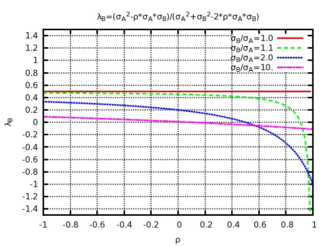
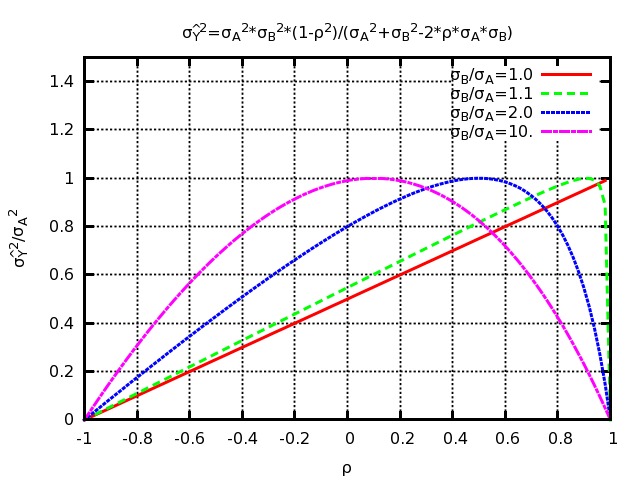
Figure 1: BLUE coefficient $\lambda_{\raisebox{-1.0pt}{\scriptsize B}}$ for measurements B (left) and combined BLUE variance $\sigma_{\raisebox{1.0pt}{\tiny$\hat{Y}$}}^{2}$ (right) as a function of the correlation $\rho$ between two measurements A and B for various fixed values of the ratio $\sigma_{\raisebox{-1.0pt}{\scriptsize B}}/\sigma_{\raisebox{-1.0pt}{\scriptsize A}}$. This is essentially the same as Fig. 1 in Ref. bib:lyons .

To better illustrate what we mean, in the bottom section of Table 1 we have added a slightly different example, where it is now assumed that $y_{\raisebox{-1.0pt}{\scriptsize B1}}$ is itself the result of the combination of two very similar measurements $y_{\raisebox{-1.0pt}{\scriptsize B11}}=99.01\pm 4.00$ and $y_{\raisebox{-1.0pt}{\scriptsize B12}}=98.99\pm 4.00$ that are 99.999% correlated to each other (and are each individually 87.5% correlated to $y_{\raisebox{-1.0pt}{\scriptsize B2}}$). It is not surprising in this case that B11 and B12 have a central value weight equal to half that of B1, an intrinsic information weight that is the same as that of B1, but a marginal information weight that is essentially zero (because including B12 is largely redundant if the almost identical measurement B11 has already been included, and viceversa). While in the combination of A, B1 and B2 the net effect of correlations was to amplify the information contribution of both B1 and B2 by $\mathrm{MIW}_{\raisebox{-1.0pt}{\scriptsize B1}}\!-\!\mathrm{IIW}_{\raisebox{-1.0pt}{\scriptsize B1}}\!=\!\mathrm{MIW}_{\raisebox{-1.0pt}{\scriptsize B2}}\!-\!\mathrm{IIW}_{\raisebox{-1.0pt}{\scriptsize B2}}\!=\!13.1\%$, in this third example the information contributions of B11 and B12 are also affected by the competing effect of their mutual correlation, which brings their $\mathrm{MIW}$ down essentially to zero. This example is also interesting because it clearly shows that very different “rankings” may be obtained for the individual measurements if they are ordered by decreasing values of $\mathrm{IIW}_{i}$, $\mathrm{MIW}_{i}$, CVW_i or $\mathrm{RI}_{i}$: for instance, measurement B11 has the highest CVW and $\mathrm{RI}$, the second highest $\mathrm{IIW}$, but the lowest $\mathrm{MIW}$. Excluding $\mathrm{RI}$, which we already argued to be an ill-defined quantity, we see in this case that CVW, $\mathrm{IIW}$ and $\mathrm{MIW}$ all have their limitations if they are used for “ranking”. Indeed, CVW can be negative, which may give the false impression that a measurement makes a combination worse instead of improving it; $\mathrm{IIW}$ completely ignores the effect of correlations; $\mathrm{MIW}$ only describes the marginal contribution of a single measurement and of its correlations. For these reasons, we propose to quote all of CVW, $\mathrm{IIW}$ and $\mathrm{MIW}$ whenever a combination of several measurements is presented, while explicitly refraining to use any of them for ranking individual measurements.

4 Negative BLUE coefficients and “high-correlation regimes”

In this section, we use the concept of Fisher information to explore the relation between negative BLUE coefficients and the size of correlations between measurements. We start by revisiting the discussion of these issues presented in Ref. bib:lyons for two measurements of one parameter, whose conclusion was that negative weights appear when the positive correlation between the two measurements exceeds a well-defined threshold. We then generalize this conclusion to $n$ measurements of one parameter, first by computing marginal information and then by analysing the derivatives of Fisher information with respect to the correlations between measurements: we show, in particular, that negative central value weights in BLUE combinations are always a sign of a “high-correlation” regime, where the marginal effect of further increasing one or more of these correlations is that of reducing the errors on the combined estimates rather than increasing them. In Sec. 5 we will discuss important practical consequences of what is presented in this section.

4.1 The simple case of two measurements of one parameter

In the simple case of two measurements A and B of a single physical quantity $Y$, the coefficients in the BLUE weighted average $\hat{Y}\!=\!\lambda_{\raisebox{-1.0pt}{\scriptsize A}}y_{\raisebox{-1.0pt}{\scriptsize A}}+\lambda_{\raisebox{-1.0pt}{\scriptsize B}}y_{\raisebox{-1.0pt}{\scriptsize B}}$ are simply given by

$$\lambda_{\raisebox{-1.0pt}{\scriptsize A}} = \frac{\sigma_{\raisebox{-1.0pt}{\scriptsize B}}^{2}-\rho\sigma_{\raisebox{-1.0pt}{\scriptsize A}}\sigma_{\raisebox{-1.0pt}{\scriptsize B}}}{\sigma_{\raisebox{-1.0pt}{\scriptsize A}}^{2}+\sigma_{\raisebox{-1.0pt}{\scriptsize B}}^{2}-2\rho\sigma_{\raisebox{-1.0pt}{\scriptsize A}}\sigma_{\raisebox{-1.0pt}{\scriptsize B}}},$$ (15)

$$\lambda_{\raisebox{-1.0pt}{\scriptsize B}} = \frac{\sigma_{\raisebox{-1.0pt}{\scriptsize A}}^{2}-\rho\sigma_{\raisebox{-1.0pt}{\scriptsize A}}\sigma_{\raisebox{-1.0pt}{\scriptsize B}}}{\sigma_{\raisebox{-1.0pt}{\scriptsize A}}^{2}+\sigma_{\raisebox{-1.0pt}{\scriptsize B}}^{2}-2\rho\sigma_{\raisebox{-1.0pt}{\scriptsize A}}\sigma_{\raisebox{-1.0pt}{\scriptsize B}}},$$ (16)

and the combined variance $\sigma_{\raisebox{1.0pt}{\tiny$\hat{Y}$}}^{2}$ (i.e. the inverse of the Fisher information) by

$$\sigma_{\raisebox{1.0pt}{\tiny$\hat{Y}$}}^{2}=\frac{\sigma_{\raisebox{-1.0pt}{\scriptsize A}}^{2}\sigma_{\raisebox{-1.0pt}{\scriptsize B}}^{2}(1-\rho^{2})}{\sigma_{\raisebox{-1.0pt}{\scriptsize A}}^{2}+\sigma_{\raisebox{-1.0pt}{\scriptsize B}}^{2}-2\rho\sigma_{\raisebox{-1.0pt}{\scriptsize A}}\sigma_{\raisebox{-1.0pt}{\scriptsize B}}}=\frac{1}{I},$$ (17)

where $\sigma_{\raisebox{-1.0pt}{\scriptsize A}}$ and $\sigma_{\raisebox{-1.0pt}{\scriptsize B}}$ are the errors on the two measurements and $\rho$ is their correlation. Assuming that the two errors are fixed, with $\sigma_{\raisebox{-1.0pt}{\scriptsize B}}>\sigma_{\raisebox{-1.0pt}{\scriptsize A}}$, the functional dependency on the correlation $\rho$ of the BLUE coefficient $\lambda_{\raisebox{-1.0pt}{\scriptsize B}}$ for measurement B and of the combined variance $\sigma_{\raisebox{1.0pt}{\tiny$\hat{Y}$}}^{2}$, given by Eq. 16 and Eq. 17 respectively, are shown in Fig.1, left and right respectively, for various values of the ratio $\sigma_{\raisebox{-1.0pt}{\scriptsize B}}/\sigma_{\raisebox{-1.0pt}{\scriptsize A}}$. For positive correlations, as discussed in Ref. bib:lyons , the combined BLUE variance increases from $\sigma_{\raisebox{1.0pt}{\tiny$\hat{Y}$}}^{2}\!=\!1/(1/\sigma_{\raisebox{-1.0pt}{\scriptsize A}}^{2}+1/\sigma_{\raisebox{-1.0pt}{\scriptsize B}}^{2})$ at $\rho\!=\!0$ to a maximum value of $\sigma_{\raisebox{1.0pt}{\tiny$\hat{Y}$}}^{2}\!=\!\sigma_{\raisebox{-1.0pt}{\scriptsize A}}^{2}$ at $\rho\!=\!\sigma_{\raisebox{-1.0pt}{\scriptsize A}}/\sigma_{\raisebox{-1.0pt}{\scriptsize B}}$ and it then decreases to $\sigma_{\raisebox{1.0pt}{\tiny$\hat{Y}$}}^{2}\!=\!0$ in the limit of $\rho\!=\!1$. Therefore, for combinations with large correlations among measurements, the combined uncertainty strongly depends on $\rho$, and is expected to vanish at $\rho\!=\!1$; this implies that, close to these regions, determining the correlation with high accuracy is mandatory so as not to bias the combination. The BLUE coefficient for B steadily decreases from $\lambda_{\raisebox{-1.0pt}{\scriptsize B}}\!=\!(1/\sigma_{\raisebox{-1.0pt}{\scriptsize B}}^{2})/(1/\sigma_{\raisebox{-1.0pt}{\scriptsize A}}^{2}+1/\sigma_{\raisebox{-1.0pt}{\scriptsize B}}^{2})$ at $\rho\!=\!0$ to a negative value of $\lambda_{\raisebox{-1.0pt}{\scriptsize B}}\!=\!-1/(\sigma_{\raisebox{-1.0pt}{\scriptsize B}}/\sigma_{\raisebox{-1.0pt}{\scriptsize A}}-1)$ in the limit of $\rho\!=\!1$, passing through $\lambda_{\raisebox{-1.0pt}{\scriptsize B}}\!=\!0$ at the correlation $\rho\!=\!\sigma_{\raisebox{-1.0pt}{\scriptsize A}}/\sigma_{\raisebox{-1.0pt}{\scriptsize B}}$ where $\sigma_{\raisebox{1.0pt}{\tiny$\hat{Y}$}}^{2}$ is maximized.

In other words, the threshold value $\rho\!=\!\sigma_{\raisebox{-1.0pt}{\scriptsize A}}/\sigma_{\raisebox{-1.0pt}{\scriptsize B}}$ effectively represents a boundary between two regimes, a “low-correlation regime”, where $\lambda_{\raisebox{-1.0pt}{\scriptsize B}}$ is positive and $\sigma_{\raisebox{1.0pt}{\tiny$\hat{Y}$}}^{2}$ increases as $\rho$ grows, and a “high-correlation regime”, where $\lambda_{\raisebox{-1.0pt}{\scriptsize B}}$ is negative and $\sigma_{\raisebox{1.0pt}{\tiny$\hat{Y}$}}^{2}$ decreases as $\rho$ grows. Note that the BLUE variance from the combination of A and B at the boundary between the two regimes $\rho\!=\!\sigma_{\raisebox{-1.0pt}{\scriptsize A}}/\sigma_{\raisebox{-1.0pt}{\scriptsize B}}$ is equal to that from A alone ($\sigma_{\raisebox{1.0pt}{\tiny$\hat{Y}$}}^{2}\!=\!\sigma_{\raisebox{-1.0pt}{\scriptsize A}}^{2}$), while it is lower on either side of the boundary. In the same way, the Fisher information from the combination at the boundary between the two regimes is equal to that from A alone, while it is higher on either side of the boundary: in other words, the marginal contribution to information from the addition of B in the combination is zero at the boundary, but it is positive on either side of it. Note in passing that the fact that the BLUE coefficient for B is zero does not mean however that the measurement is simply not used in the combination, because the central value measured by B does in any case contribute to the calculation of the overall $\chi^{2}$ for the combination: this statement remains valid for the combination of $n$ measurements, although we will not repeat it in the following.

A possible interpretation of the transition at $\rho\!=\!\sigma_{\raisebox{-1.0pt}{\scriptsize A}}/\sigma_{\raisebox{-1.0pt}{\scriptsize B}}$, which will become useful later on and is complementary to that given in Ref. bib:lyons (as well as to that given in Ref. bib:cox using the Cholesky decomposition formalism), is the following. In the low-correlation regime $\rho\leq\sigma_{\raisebox{-1.0pt}{\scriptsize A}}/\sigma_{\raisebox{-1.0pt}{\scriptsize B}}$, the full covariance matrix can be written as the sum of two positive-definite components: one that is common to A and B, i.e. 100% correlated and with the same size in both, and one that is uncorrelated:

$$\biggl{(}\begin{array}[]{cc}\sigma_{\raisebox{-1.0pt}{\scriptsize A}}^{2}&\,\rho\sigma_{\raisebox{-1.0pt}{\scriptsize A}}\sigma_{\raisebox{-1.0pt}{\scriptsize B}}\\ \,\rho\sigma_{\raisebox{-1.0pt}{\scriptsize A}}\sigma_{\raisebox{-1.0pt}{\scriptsize B}}&\sigma_{\raisebox{-1.0pt}{\scriptsize B}}^{2}\\ \end{array}\biggr{)}=\biggl{(}\begin{array}[]{cc}\,\rho\sigma_{\raisebox{-1.0pt}{\scriptsize A}}\sigma_{\raisebox{-1.0pt}{\scriptsize B}}&\,\rho\sigma_{\raisebox{-1.0pt}{\scriptsize A}}\sigma_{\raisebox{-1.0pt}{\scriptsize B}}\\ \,\rho\sigma_{\raisebox{-1.0pt}{\scriptsize A}}\sigma_{\raisebox{-1.0pt}{\scriptsize B}}&\,\rho\sigma_{\raisebox{-1.0pt}{\scriptsize A}}\sigma_{\raisebox{-1.0pt}{\scriptsize B}}\\ \end{array}\biggr{)}_{\mathrm{com}}\\ +\biggl{(}\begin{array}[]{cc}\,\sigma_{\raisebox{-1.0pt}{\scriptsize A}}^{2}\!-\!\rho\sigma_{\raisebox{-1.0pt}{\scriptsize A}}\sigma_{\raisebox{-1.0pt}{\scriptsize B}}&0\\ 0&\,\sigma_{\raisebox{-1.0pt}{\scriptsize B}}^{2}\!-\!\rho\sigma_{\raisebox{-1.0pt}{\scriptsize A}}\sigma_{\raisebox{-1.0pt}{\scriptsize B}}\\ \end{array}\biggr{)}_{\mathrm{unc}}.$$ (18)

Indeed, only when the off-diagonal covariance $\rho\sigma_{\raisebox{-1.0pt}{\scriptsize A}}\sigma_{\raisebox{-1.0pt}{\scriptsize B}}$ is smaller than both variances $\sigma_{\raisebox{-1.0pt}{\scriptsize A}}^{2}$ and $\sigma_{\raisebox{-1.0pt}{\scriptsize B}}^{2}$ can the “uncorrelated” error component be positive definite. The possibility to split the covariance matrix in this way can be interpreted by saying that, in the low-correlation regime, the marginal information added to the combination by the less precise measurement B comes from its contribution of independent (uncorrelated) knowledge about the unknown parameter. To combine A and B in this case, in fact, one may simply think of temporarely ignoring the irreducible common component of the error, combining the two measurements based only on the uncorrelated error components and finally adding back the common error component: it is easy to see that this would lead to a total combined variance

$$\sigma_{\raisebox{1.0pt}{\tiny$\hat{Y}$}}^{2}=\biggl{(}\rho\sigma_{\raisebox{-1.0pt}{\scriptsize A}}\sigma_{\raisebox{-1.0pt}{\scriptsize B}}\biggr{)}_{\mathrm{com}}\\ +\biggl{(}\frac{\sigma_{\raisebox{-1.0pt}{\scriptsize A}}\sigma_{\raisebox{-1.0pt}{\scriptsize B}}(\sigma_{\raisebox{-1.0pt}{\scriptsize A}}\!-\!\rho\sigma_{\raisebox{-1.0pt}{\scriptsize B}})(\sigma_{\raisebox{-1.0pt}{\scriptsize B}}\!-\!\rho\sigma_{\raisebox{-1.0pt}{\scriptsize A}})}{\sigma_{\raisebox{-1.0pt}{\scriptsize A}}^{2}+\sigma_{\raisebox{-1.0pt}{\scriptsize B}}^{2}-2\rho\sigma_{\raisebox{-1.0pt}{\scriptsize A}}\sigma_{\raisebox{-1.0pt}{\scriptsize B}}}\biggr{)}_{\mathrm{unc}},$$ (19)

which adds up to the same value given in Eq. 17. With respect to the measurement of A taken alone, adding B helps in this case by reducing the uncorrelated error component (the second term on the right-hand side).

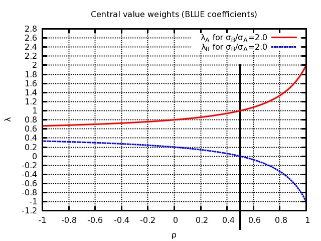
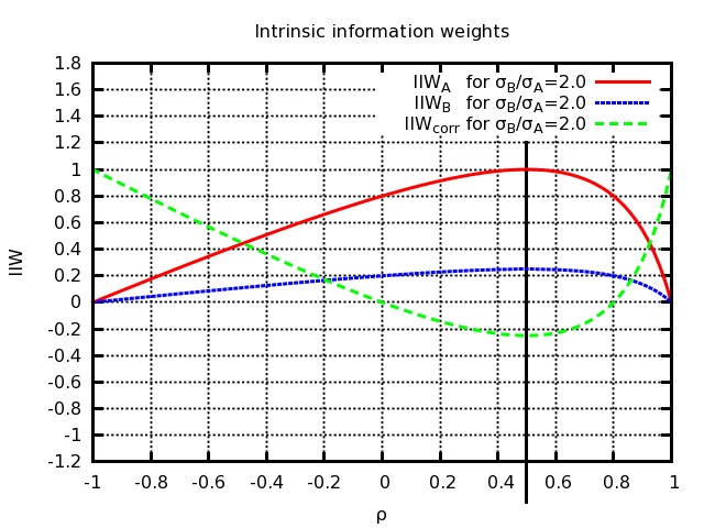
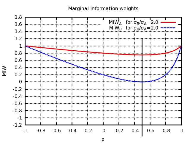
Figure 2: BLUE coefficients $\lambda$ for A and B (top left), intrinsic information weights $\mathrm{IIW}$ for A, B and correlations (top right), marginal information weights $\mathrm{MIW}$ for A and B (bottom left) and relative importances $\mathrm{RI}$ for A and B (bottom right) as a function of the correlation $\rho$ between A and B for the specific example $\sigma_{\raisebox{-1.0pt}{\scriptsize B}}/\sigma_{\raisebox{-1.0pt}{\scriptsize A}}$=2. The black line in each plot indicates the boundary between low-correlation and high-correlation regimes at $\rho\!=\!1/2$ where the total information from A and B is minimized.

In the high correlation regime, conversely, the covariance matrix can not be seen as the sum of a common error and an uncorrelated error as in Eq. 18. Instead, the full covariance matrix can be written as the sum of a component common to A and B, i.e. 100% correlated and with the same size in both, and of another systematic effect that is also 100% correlated, but has different sizes in A and B:

$$\biggl{(}\begin{array}[]{cc}\sigma_{\raisebox{-1.0pt}{\scriptsize A}}^{2}&\,\rho\sigma_{\raisebox{-1.0pt}{\scriptsize A}}\sigma_{\raisebox{-1.0pt}{\scriptsize B}}\\ \,\rho\sigma_{\raisebox{-1.0pt}{\scriptsize A}}\sigma_{\raisebox{-1.0pt}{\scriptsize B}}&\sigma_{\raisebox{-1.0pt}{\scriptsize B}}^{2}\\ \end{array}\biggr{)}=\biggl{(}\begin{array}[]{cc}\sigma_{\raisebox{1.0pt}{\tiny$\hat{Y}$}}^{2}&\sigma_{\raisebox{1.0pt}{\tiny$\hat{Y}$}}^{2}\\ \sigma_{\raisebox{1.0pt}{\tiny$\hat{Y}$}}^{2}&\sigma_{\raisebox{1.0pt}{\tiny$\hat{Y}$}}^{2}\\ \end{array}\biggr{)}_{\mathrm{com}}\\ +(\sigma_{\raisebox{-1.0pt}{\scriptsize A}}^{2}+\sigma_{\raisebox{-1.0pt}{\scriptsize B}}^{2}-2\rho\sigma_{\raisebox{-1.0pt}{\scriptsize A}}\sigma_{\raisebox{-1.0pt}{\scriptsize B}})\biggl{(}\begin{array}[]{cc}\lambda_{\raisebox{-1.0pt}{\scriptsize B}}^{2}&-\lambda_{\raisebox{-1.0pt}{\scriptsize A}}\lambda_{\raisebox{-1.0pt}{\scriptsize B}}\\ -\lambda_{\raisebox{-1.0pt}{\scriptsize A}}\lambda_{\raisebox{-1.0pt}{\scriptsize B}}&\lambda_{\raisebox{-1.0pt}{\scriptsize A}}^{2}\\ \end{array}\biggr{)}_{\mathrm{cor}}.$$ (20)

In the combined result, the total error $\sigma_{\raisebox{1.0pt}{\tiny$\hat{Y}$}}$ comes exclusively from the common systematic uncertainty in the first component, while the contribution from the correlated systematic uncertainty in the second component is 0. In other words,

$$\sigma_{\raisebox{1.0pt}{\tiny$\hat{Y}$}}^{2}=\biggl{(}\sigma_{\raisebox{1.0pt}{\tiny$\hat{Y}$}}^{2}\bigg{)}_{\mathrm{com}}+\biggl{(}0\biggr{)}_{\mathrm{cor}},$$ (21)

which can again be seen by removing the common component, combining and then adding it back at the end. For all practical purposes, one can thus say that, in the high correlation regime, the marginal information added by the less precise measurement B does not come from independent knowledge it contributes about the unknown parameter, but from its ability to constrain and remove a systematic uncertainty that also affects A, but to which B has a larger sensitivity. With respect to the measurement of A taken alone, in fact, adding B helps by completely getting rid of the correlated error component (the second term on the right-hand side). Note also, as discussed in Refs. bib:lyons ; bib:cox , that the two individual measurements A and B are on the same side of the combined estimate in the high correlation regime (unless they coincide), because $\lambda_{\raisebox{-1.0pt}{\scriptsize B}}\!<\!0$ implies that $\hat{Y}\!<\!y_{\raisebox{-1.0pt}{\scriptsize A}}\!<\!y_{\raisebox{-1.0pt}{\scriptsize B}}$ or $y_{\raisebox{-1.0pt}{\scriptsize B}}\!<\!y_{\raisebox{-1.0pt}{\scriptsize A}}\!<\!\hat{Y}$.

To further illustrate this difference between the low and high correlation regimes, it is interesting to study the functional dependency on the correlation $\rho$ of the intrinsic and marginal information weights $\mathrm{IIW}$ and $\mathrm{MIW}$ that we introduced in Sec. 3. In Fig. 2 we compare the functional dependencies on $\rho$ of the BLUE coefficients $\lambda$, intrinsic information weights $\mathrm{IIW}$, marginal information weights $\mathrm{MIW}$ and relative importances $\mathrm{RI}$ for one specific example where $\sigma_{\raisebox{-1.0pt}{\scriptsize B}}/\sigma_{\raisebox{-1.0pt}{\scriptsize A}}\!=\!2$. As expected, both the intrinsic and marginal information weights of the two individual measurements are non-negative and actually coincide with each other and with the BLUE coefficients when $\rho\!=\!0$, while they have two maxima and two minima, respectively, at the boundary between low-correlation and high-correlation regimes at $\rho\!=\!\sigma_{A}/\sigma_{B}$ where the total information from A and B is minimized. In the limit of extremely high correlation $\rho\!=\!1$, where the combined variance tends to 0 as the information contributed by the correlation between the two measurements tends to infinity, the intrinsic information weights tend to 0 while the marginal information weights tend to 1, because the intrinsic information contributed by each experiment individually is negligible with respect to the large contribution they achieve together through their correlation. For comparison, note instead that the “relative importances” of A and B at $\rho\!=\!1$ are both positive and sum up to 1 while being different from each other, which in our opinion is another indication that this concept fails to acknowledge the relevance here of the information contribution from correlations.

4.2 Marginal information from the $i^{\mathrm{th}}$ measurement of one parameter

To generalize the concepts of low and high correlation regimes, and show their relation to negative BLUE coefficients, in the more general case of $n$ measurements of one parameter, we now derive formulas to calculate the marginal information $\Delta I_{i}$ of the $i^{\mathrm{th}}$ measurement in an $n$-measurement combination, using the “information inflow” formalism of Ref. bib:bos . Without loss of generality, imagine that the $n$ measurements in the combination are reordered so that the $i^{\mathrm{th}}$ measurement we are interested in becomes the last, i.e. the $n^{\mathrm{th}}$, measurement. The full covariance matrix for all $n$ measurements can then be written as

$$\mathcal{M}=\left(\begin{array}[]{cc}\mathcal{D}&\mathbf{c}\\ \tilde{\mathbf{c}}&d\\ \end{array}\right),$$ (22)

where the variance of the $i^{\mathrm{th}}$ measurement is given by $\sigma_{i}^{2}\!=\!d$, its covariances with all other measurements are the $(n\!-\!1)$ elements of the vector $\mathbf{c}$, and $\mathcal{D}$ is the $(n\!-\!1)\!\times\!(n\!-\!1)$ covariance matrix of these $n\!-\!1$ other measurements. Using Frobenius’ formula bib:bos , the inverse of this matrix can be written as

$$\mathcal{M}^{-1}=\left(\begin{array}[]{cc}\hskip 5.69046pt\mathcal{D}^{-1}+\frac{\left(\mathcal{D}^{-1}\mathbf{c}\right)\left(\tilde{\mathbf{c}}\mathcal{D}^{-1}\right)}{\raisebox{-2.0pt}{$d-(\tilde{\mathbf{c}}\mathcal{D}^{-1}\mathbf{c})$}}&\hskip 5.69046pt\frac{-\left(\mathcal{D}^{-1}\mathbf{c}\right)}{\raisebox{-2.0pt}{$d-(\tilde{\mathbf{c}}\mathcal{D}^{-1}\mathbf{c})$}}\\ \hskip 5.69046pt\frac{-\left(\tilde{\mathbf{c}}\mathcal{D}^{-1}\right)}{\raisebox{-2.0pt}{$d-(\tilde{\mathbf{c}}\mathcal{D}^{-1}\mathbf{c})$}}&\hskip 5.69046pt\frac{1}{\raisebox{-2.0pt}{$d-(\tilde{\mathbf{c}}\mathcal{D}^{-1}\mathbf{c})$}}\\ \end{array}\right),$$ (23)

where $1/(d-(\tilde{\mathbf{c}}\mathcal{D}^{-1}\mathbf{c}))>0$ because it is a diagonal element of the inverse of the symmetric positive definite matrix $\mathcal{M}$. Keeping in mind that the information $I$ from the combination of $n$ measurements according to Eq. 9 is simply $\tilde{\mathbf{U}}\mathcal{M}^{-1}\mathbf{U}$, it can easily be shown bib:bos that the marginal information $\Delta I_{i}$ (or information inflow) from the $i^{\mathrm{th}}$ measurement is given by

$$\Delta I_{i}=\frac{\left((\tilde{\mathbf{u}}\mathcal{D}^{-1}\mathbf{c})-1\right)^{2}}{d-(\tilde{\mathbf{c}}\mathcal{D}^{-1}\mathbf{c})}\geq 0,$$ (24)

where $\mathbf{u}$ is a vector whose $(n\!-\!1)$ elements are all equal to 1 (i.e. the equivalent of $\mathbf{U}$, but with one less measurement).

Let us now analyze this formula, assuming that the covariance matrix $\mathcal{D}$ of the other $(n\!-\!1)$ measurements and the variance $d$ of the $i^{\mathrm{th}}$ measurement are both fixed, while the $(n\!-\!1)$ correlations in $\mathbf{c}$ can vary. We then observe that the condition $\Delta I_{i}\!=\!0$, where information has a minimum, corresponds to a hyperplane in the $(n\!-\!1)$-dimensional space of these correlations, defined by

$$\Delta I_{i}=0\iff(\tilde{\mathbf{u}}\mathcal{D}^{-1}\mathbf{c})-1=0.$$ (25)

This hyperplane divides the $(n\!-\!1)$-dimensional space of correlations into two half-spaces: a half-space containing the origin $\mathbf{c}\!=\!\mathbf{0}$ (i.e. the point where there are no correlations), which we will therefore call the “low-correlation” regime; and a half-space that does not contain the origin, which we will call the “high-correlation” regime, defined by

$$(\tilde{\mathbf{u}}\mathcal{D}^{-1}\mathbf{c})-1\geq 0.$$ (26)

Keeping in mind that the BLUE coefficients are given by Eq. 1, i.e. by

$$\bm{\tilde{\lambda}}=\frac{\tilde{\mathbf{U}}\mathcal{M}^{-1}}{I},$$ (27)

and substituting $\mathcal{M}^{-1}$ by the expression in Eq. 23, we observe that the BLUE coefficient for the $i^{\mathrm{th}}$ measurement is

$$\lambda_{i}=-\frac{1}{I}\times\frac{(\tilde{\mathbf{u}}\mathcal{D}^{-1}\mathbf{c})-1}{d-(\tilde{\mathbf{c}}\mathcal{D}^{-1}\mathbf{c})}.$$ (28)

Having already observed that $(d-(\tilde{\mathbf{c}}\mathcal{D}^{-1}\mathbf{c}))>0$, this implies that

$$\lambda_{i}\leq 0\iff(\tilde{\mathbf{u}}\mathcal{D}^{-1}\mathbf{c})-1\geq 0.$$ (29)

Comparing this to Eq. 26, this shows that the condition $\lambda_{i}\leq 0$ coincides with that defining the half-space corresponding to the “high-correlation” regime. In other words, the BLUE coefficient for the $i^{\mathrm{th}}$ measurement is negative if and only if its correlations to the other $n\!-\!1$ measurements are higher than the thresholds for crossing over into the high-correlation regime; it is instead zero on the boundary between the two regimes, i.e. if and only if these correlations are such that the measurement contributes no additional information to the combination.

The results presented above are interesting not only to point out the relation between negative BLUE coefficients and high-correlation regimes, but also because they provide a formula for computing marginal information weights. For the $i^{\mathrm{th}}$ measurement, this is simply equal to

$$\mathrm{MIW}_{i}=\frac{\Delta I_{i}}{I}=\frac{1}{I}\times\frac{\left((\tilde{\mathbf{u}}\mathcal{D}^{-1}\mathbf{c})-1\right)^{2}}{d-(\tilde{\mathbf{c}}\mathcal{D}^{-1}\mathbf{c})}=\lambda_{i}^{2}I\left(d-(\tilde{\mathbf{c}}\mathcal{D}^{-1}\mathbf{c})\right).$$ (30)

Keeping in mind that the intrinsic information weight for the same measurement is $\mathrm{IIW}_{i}=(1/\sigma_{i}^{2})/I=1/dI$, this implies that

$$\mathrm{MIW}_{i}\ \times\ \mathrm{IIW}_{i}=\lambda_{i}^{2}\left(1-\frac{(\tilde{\mathbf{c}}\mathcal{D}^{-1}\mathbf{c})}{d}\right)\leq\lambda_{i}^{2},$$ (31)

which provides an interesting relationship between intrinsic information weights, marginal information weights and central value weights. Note, in particular, that the equality sign holds if the $i^{\mathrm{th}}$ measurement is not correlated to any other measurements (i.e. if $\mathbf{c}$ is the null vector), in which case all three weights coincide as seen in Table 1.

4.3 Information derivatives

In the first part of this section, we have described the boundary between low-correlation and high-correlation regimes in the simplest case of the combination of two measurements, as well as in the more complex but still specific case of the combination of $n$ measurements, where only the $n\!-\!1$ correlations of the $i^{\mathrm{th}}$ measurement to all of the others are allowed to vary. We now analyze the most general case of the combination of $n$ measurements of one parameter, as a function of the $n(n\!-\!1)/2$ correlations of all the measurements to one another. We do this by studying the first derivatives of information with respect to these correlations $\rho_{ij}$.

Let us consider the linear dependency of the covariance matrix $\mathcal{M}$ on the $n(n\!-\!1)/2$ correlations $\rho_{ij}$ between any two distinct measurements $y_{i}$ and $y_{j}$, assuming instead that the variances $\mathcal{M}_{ii}$ are fixed. Applying the generic formula bib:bos for the first derivatives of the inverse of a non-singular square matrix with respect to the elements of a vector it depends on, we find that

$$\frac{\partial\mathcal{M}^{-1}}{\partial\rho_{ij}}=-\mathcal{M}^{-1}\frac{\partial\mathcal{M}}{\partial\rho_{ij}}\mathcal{M}^{-1}.$$ (32)

Keeping in mind that $I=\tilde{\mathbf{U}}\mathcal{M}^{-1}\mathbf{U}$ and that $\tilde{\mathbf{U}}\mathcal{M}^{-1}=I\bm{\tilde{\lambda}}$ according to Eqs. 9 and 27, respectively, the derivatives of information with respect to the correlations $\rho_{ij}$ can be written as

$$\frac{\partial I}{\partial\rho_{ij}}=-\tilde{\mathbf{U}}\mathcal{M}^{-1}\frac{\partial\mathcal{M}}{\partial\rho_{ij}}\mathcal{M}^{-1}\mathbf{U}=-I^{2}\bm{\tilde{\lambda}}\frac{\partial\mathcal{M}}{\partial\rho_{ij}}\bm{\lambda}.$$ (33)

Under our assumption that only the off-diagonal covariances $\mathcal{M}_{ij}$ may vary while the variances $\mathcal{M}_{ii}$ are fixed, the derivatives of the covariance matrix $\mathcal{M}$ with respect to the correlations $\rho_{ij}$ are

$$\begin{split}\left(\frac{\partial\mathcal{M}}{\partial\rho_{ij}}\right)_{kl}&=\sqrt{\mathcal{M}_{ii}}\sqrt{\mathcal{M}_{jj}}\times\left(\delta_{il}\delta_{jk}+\delta_{ik}\delta_{jl}\right)\\ &=\sqrt{\mathcal{M}_{ii}}\sqrt{\mathcal{M}_{jj}}\times\left\{\begin{array}[]{ll}1&\mathrm{if}\,i=k\,\mathrm{and}\,j=l\,,\\ 1&\mathrm{if}\,i=l\,\mathrm{and}\,j=k\,,\\ 0&\mathrm{otherwise}\,.\end{array}\right.\end{split}$$ (34)

The derivatives of information with respect to the correlations $\rho_{ij}$ are then simply given by

$$\frac{\partial I}{\partial\rho_{ij}}=-2I^{2}\lambda_{i}\lambda_{j}\sqrt{\mathcal{M}_{ii}}\sqrt{\mathcal{M}_{jj}},$$ (35)

where the factor 2 comes from the fact that the covariance matrix is symmetric and has twice as many off-diagonal elements as there are independent correlations.

Equation 35 clearly shows that, if all BLUE coefficients are positive, the first derivatives of information are always negative with respect to the correlations between any two measurements, i.e. information can only decrease if correlations are further increased: this is the equivalent in $n(n\!-\!1)/2$ dimensional space of what we have previously called a “low-correlation” regime, as this sub-space is guaranteed to contain the point where all correlations are zero. Conversely, if at least one BLUE coefficient is negative (and keeping in mind that they can not be all negative), then at least one information derivative must be positive, i.e. there is at least one correlation which leads to higher information if it is increased: this is the equivalent of what we have previously called a “high-correlation” regime. The boundary between the two regimes is a hypersurface in $n(n\!-\!1)/2$ dimensional space, defined by the condition that at least one BLUE coefficient is zero, while all the others are non-negative: when this condition is satisfied, the information derivatives with respect to one or more correlations are also zero, meaning that information has reached a minimum in its partial functional dependency on those correlations. This completes the generalization to several measurements of one observable of the discussion presented in Ref. bib:lyons for only two measurements. Note finally that in that case, i.e. for $n\!=\!2$, all these considerations are trivially illustrated by Figures 1 and 2, showing that the boundary between low and high correlation regimes in the 1-dimensional space of the correlation $\rho$ is a 0-dimensional hypersurface (a point) at the value $\rho=\sigma_{\raisebox{-1.0pt}{\scriptsize A}}/\sigma_{\raisebox{-1.0pt}{\scriptsize B}}$.

5 “Conservative” estimates of correlations in BLUE combinations

A precise assessment of the correlations that need to be used as input to BLUE combinations is often very hard. Ideally, one should aim to measure these correlations in the data or by using Monte Carlo methods. This, however, turns out to be often impractical, if not impossible, for instance when combining results produced by different experiments that use different conventions for assessing the systematic errors on their measurements, or when trying to combine results from recent experiments to older results for which not enough details were published and the expertise and the infrastructure to analyse the data are no longer available. In these situations, it may be unavoidable to combine results using input covariance matrices where the correlations between the different measurements have only been approximately estimated, rather than accurately measured. In the following, we will refer to these estimates of correlations as the “nominal” correlations (and we will extensively study the effect on BLUE combination results of reducing correlations below these initial “nominal” values).

In particular, it is not uncommon to read in the literature that correlations have been “conservatively” assumed to be 100%. In this section, we question the validity of this kind of statement. A “conservative” estimate of a measurement error should mean that, in the absence of more precise assessments, an overestimate of the true error (at the price of losing some of the available information from a measurement) is more acceptable than taking the risk of claiming that a measurement is more accurate than it really is. Likewise, by “conservative” estimate of a correlation, one should mean an estimate which is more likely to result in an overall larger combined error than in a wrong claim of smaller combined errors.

When BLUE coefficients are all positive, i.e. in a low-correlation regime, information derivatives are negative and the net effect of increasing any correlation can only be that of reducing information and increasing the combined error: in this case, choosing the largest possible positive correlations (100%) is clearly the most conservative choice. Our discussion in the previous section, however, shows that negative BLUE coefficients are a sign of a high-correlation regime, where the net effect of increasing some of these correlations is that of increasing information and reducing the combined error: in other words, if correlations are estimated as 100% and negative BLUE coefficients are observed, it is wrong to claim that correlations have been estimated “conservatively”.

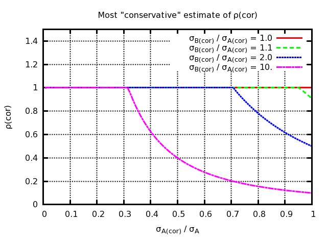
Figure 3: Most “conservative” value of an unknown correlation $\rho_{\mathrm{cor}}$ between $\sigma_{A(\mathrm{cor})}$ and $\sigma_{B(\mathrm{cor})}$ as a function of $\sigma_{A(\mathrm{cor})}/\sigma_{\raisebox{-1.0pt}{\scriptsize A}}$, for several values of $\sigma_{B(\mathrm{cor})}/\sigma_{A(\mathrm{cor})}\geq 1$.

In this section, we will first analyse under which conditions it is indeed conservative to assume that correlations are 100%, using a simple two-measurement combination as an example. For those situations where a precise evaluation of correlations is impossible, and where setting them to their “nominal” estimates would result in negative BLUE coefficients, we will then offer a few guidelines and tools to help physicists make more conservative estimates of correlations.

5.1 Conservative estimates of correlations in a two-measurement combination

Let us consider the combination of two measurements A and B, whose errors are well known, but where the correlation $\rho$ between them could not be precisely determined. We want to determine in this case which would be the most “conservative” estimate for $\rho$. We do this by studying the functional dependency of the total combined error on $\rho$ (which throughout this Sec. 5.1 is taken as a variable parameter, rather than any “nominal” estimate of the correlation). We observed in Sec. 4.1 that this combination remains in a low-correlation regime as long as the off-diagonal covariance $\rho\sigma_{\raisebox{-1.0pt}{\scriptsize A}}\sigma_{\raisebox{-1.0pt}{\scriptsize B}}$ is smaller than both variances $\sigma_{\raisebox{-1.0pt}{\scriptsize A}}^{2}$ and $\sigma_{\raisebox{-1.0pt}{\scriptsize B}}^{2}$,

$$\biggl{\{}\begin{array}[]{ccc}\rho\sigma_{\raisebox{-1.0pt}{\scriptsize A}}\sigma_{\raisebox{-1.0pt}{\scriptsize B}}&\leq&\sigma_{\raisebox{-1.0pt}{\scriptsize A}}^{2},\\ \rho\sigma_{\raisebox{-1.0pt}{\scriptsize A}}\sigma_{\raisebox{-1.0pt}{\scriptsize B}}&\leq&\sigma_{\raisebox{-1.0pt}{\scriptsize B}}^{2}.\\ \end{array}\biggr{.}$$ (36)

Let us now assume that there are only two sources of uncertainty, an uncorrelated error $\sigma_{\mathrm{(unc)}}$, e.g. of statistical origin, and a single systematic effect $\sigma_{\mathrm{(cor)}}$ whose correlation between the two measurements is $\rho_{\mathrm{cor}}$. The most conservative estimate for $\rho_{\mathrm{cor}}$ according to Eq. 36 above is thus the largest value of $\rho_{\mathrm{cor}}$ such that

$$\biggl{\{}\begin{array}[]{ccc}\rho\sigma_{\raisebox{-1.0pt}{\scriptsize A}}\sigma_{\raisebox{-1.0pt}{\scriptsize B}}=\rho_{\mathrm{cor}}\sigma_{A(\mathrm{cor})}\sigma_{B(\mathrm{cor})}&\leq&(\sigma_{A(\mathrm{unc})}^{2}+\sigma_{A(\mathrm{cor})}^{2})=\sigma_{\raisebox{-1.0pt}{\scriptsize A}}^{2},\\ \rho\sigma_{\raisebox{-1.0pt}{\scriptsize A}}\sigma_{\raisebox{-1.0pt}{\scriptsize B}}=\rho_{\mathrm{cor}}\sigma_{A(\mathrm{cor})}\sigma_{B(\mathrm{cor})}&\leq&(\sigma_{B(\mathrm{unc})}^{2}+\sigma_{B(\mathrm{cor})}^{2})=\sigma_{\raisebox{-1.0pt}{\scriptsize B}}^{2}.\\ \end{array}\biggr{.}$$ (37)

This expression is very interesting because it is automatically satisfied by any value of $\rho_{\mathrm{cor}}$ for measurements that are statistically dominated, i.e. where each of $\sigma_{A(\mathrm{unc})}$ and $\sigma_{B(\mathrm{unc})}$ is much larger than both $\sigma_{A(\mathrm{cor})}$ and $\sigma_{B(\mathrm{cor})}$: in other words, for statistically dominated measurements, it is indeed a correct statement to say that “correlations are conservatively assumed to be 100%”.

If the measurements are not statistically dominated, however, the situation is different. Taking $\sigma_{A(\mathrm{cor})}$ to be the smaller of the two correlated errors, i.e. $\sigma_{A(\mathrm{cor})}\leq\sigma_{B(\mathrm{cor})}$, then the second condition is automatically true, while the first condition is satisfied if and only if

$$\rho_{\mathrm{cor}}\leq\frac{\sigma_{\raisebox{-1.0pt}{\scriptsize A}}^{2}}{\sigma_{A(\mathrm{cor})}\sigma_{B(\mathrm{cor})}}=\frac{\sigma_{A(\mathrm{cor})}/\sigma_{B(\mathrm{cor})}}{(\sigma_{A(\mathrm{cor})}/\sigma_{\raisebox{-1.0pt}{\scriptsize A}})^{2}}.$$ (38)

This shows that, when systematic errors cannot be ignored and the sensitivities of A and B to the correlated systematic effect are so different that $(\sigma_{B(\mathrm{cor})}/\sigma_{A(\mathrm{cor})})\geq(\sigma_{\raisebox{-1.0pt}{\scriptsize A}}/\sigma_{A(\mathrm{cor})})^{2}$, then it is no longer correct to take 100% as the most conservative value of $\rho_{\mathrm{cor}}$, and one must choose a correlation that is smaller than 100%. This is shown in Fig. 3, where the most conservative value of $\rho_{\mathrm{cor}}$ is plotted as a function of $\sigma_{A(\mathrm{cor})}/\sigma_{\raisebox{-1.0pt}{\scriptsize A}}$, for several values of $\sigma_{B(\mathrm{cor})}/\sigma_{A(\mathrm{cor})}$.

This figure shows that there are two different regimes. When $(\sigma_{B(\mathrm{cor})}/\sigma_{A(\mathrm{cor})})<(\sigma_{\raisebox{-1.0pt}{\scriptsize A}}/\sigma_{A(\mathrm{cor})})^{2}$, the most conservative value of $\rho_{\mathrm{cor}}$ is 1: in this case, both measurements A and B contribute to the combination with positive BLUE coefficients because, no matter how large $\rho_{\mathrm{cor}}$ is, the combination always remains in a low-correlation regime. When $(\sigma_{B(\mathrm{cor})}/\sigma_{A(\mathrm{cor})})\geq(\sigma_{\raisebox{-1.0pt}{\scriptsize A}}/\sigma_{A(\mathrm{cor})})^{2}$, instead, the most conservative value of $\rho_{\mathrm{cor}}$ is smaller than 1: in this case, the combination is at the boundary of low and high correlation regimes, where the combined error is maximised and equal to $\sigma_{\raisebox{1.0pt}{\tiny$\hat{Y}$}}\!=\!\sigma_{\raisebox{-1.0pt}{\scriptsize A}}$ while $\lambda_{A}\!=\!1$ and $\lambda_{B}\!=\!0$, which is more or less equivalent (modulo the effect on $\chi^{2}$ previously discussed) to excluding the less precise measurement B from the combination.

5.2 Identifying the least conservative correlations between $n$ measurements

While it is relatively straightforward to determine the “most conservative” estimate of correlations with only two measurements, things get more complicated when the combination includes $n$ measurements, as the number of inter-measurement correlations increases to $n(n\!-\!1)/2$ and the “most conservative” value for any of them would depend on the values of the others. Instead of treating all correlations as completely free parameters as we did in Sec. 5.1, throughout this Sec. 5.2 we will then suggest ways to analyse how “conservative” an existing “nominal” estimate of correlations is. In particular, we will consider the most general case where the full “nominal” covariance matrix is built as the sum of $S$ sources of uncertainty, each with a different set of “nominal” correlations between the measurements,

$$\mathcal{M}_{ij}=\sum_{s=1}^{S}\mathcal{M}^{\raisebox{0.0pt}{{$[$}\scriptsize$s${$]$}}}_{ij}=\sum_{s=1}^{S}\left\{\begin{array}[]{ll}\mathcal{M}^{\raisebox{0.0pt}{{$[$}\scriptsize$s${$]$}}}_{ii}&\hskip 5.69054pt\mathrm{if}\,\,i=j,\\ \rho_{ij}^{\raisebox{0.0pt}{{$[$}\scriptsize$s${$]$}}}\sqrt{\mathcal{M}^{\raisebox{0.0pt}{{$[$}\scriptsize$s${$]$}}}_{ii}}\sqrt{\mathcal{M}^{\raisebox{0.0pt}{{$[$}\scriptsize$s${$]$}}}_{jj}}&\hskip 5.69054pt\mathrm{if}\,\,i\neq{j}.\\ \end{array}\right.$$ (39)

If the “nominal” values of the correlations $\rho_{ij}^{\raisebox{0.0pt}{{$[$}\scriptsize$s${$]$}}}$ are not assessed rigorously and it is still conceivable to modify them to make the combination more “conservative”, it is certainly useful to know which of these correlations correspond to a high correlation regime and which of them contribute more significantly to a change in the combined error. To answer the first question, one should look at the correlations of those measurements whose BLUE coefficients are negative in the “nominal” combination. In particular, one should concentrate on the correlations $\rho_{ij}$ between two measurements $y_{i}$ and $y_{j}$ such that the derivatives $\partial I/\partial\rho_{ij}$ in Eq. 35 are positive. To answer the second question, we propose to use the information derivatives we derived in Sec. 4.3 and look at which correlation would yield the largest relative decrease of information $\delta I/I$ for the same relative rescaling downwards $\delta\rho_{ij}^{\raisebox{0.0pt}{{$[$}\scriptsize$s${$]$}}}/\rho_{ij}^{\raisebox{0.0pt}{{$[$}\scriptsize$s${$]$}}}$ of that correlation. In other words, we suggest to rank correlations by the normalised information derivative

$$\frac{\rho_{ij}^{\raisebox{0.0pt}{{$[$}\scriptsize$s${$]$}}}}{I}\left(\frac{\partial I}{\partial\rho_{ij}^{\raisebox{0.0pt}{{$[$}\scriptsize$s${$]$}}}}\right)=-2I\lambda_{i}\lambda_{j}\rho_{ij}^{\raisebox{0.0pt}{{$[$}\scriptsize$s${$]$}}}\sqrt{\mathcal{M}_{ii}^{\raisebox{0.0pt}{{$[$}\scriptsize$s${$]$}}}}\sqrt{\mathcal{M}_{jj}^{\raisebox{0.0pt}{{$[$}\scriptsize$s${$]$}}}}=-2\,\frac{\lambda_{i}\lambda_{j}\mathcal{M}_{ij}^{\raisebox{0.0pt}{{$[$}\scriptsize$s${$]$}}}}{\sigma_{\raisebox{1.0pt}{\tiny$\hat{Y}$}}^{2}},$$ (40)

where all quantities in the formula (which is easily derived by extending Eq. 33) are computed at the “nominal” values of the correlations. The correlations between measurements $i$ and $j$ and for error source $s$ with the highest positive values of the normalized derivative in Eq. 40 are those that should be most urgently reassessed. The quantity in Eq. 40 is a dimensionless number: in the simple example presented in Sec. 2, for instance, the value of this normalised derivative for the correlation between B1 and B2 (for the single source of uncertainty considered in that example) is as high as +2.52, indicating that the combined error would increase by 2.52% for a relative reduction of the correlation by 1% of its “nominal” value (from 0.87500 to 0.86625). We will illustrate this in more detail at the end of this section using a numerical example.

Note that the sums of all $(\rho_{ij}^{\raisebox{0.0pt}{{$[$}\scriptsize$s${$]$}}}/I)(\partial I/\partial\rho_{ij}^{\raisebox{0.0pt}{{$[$}\scriptsize$s${$]$}}})$ over all error sources $s$ effectively represent the effect on information of rescaling the correlations between measurements $i$ and $j$ by the same factor for all error sources, while their sums over measurements $i$ and $j$ represent the effect of rescaling the correlations between all measurements by the same factor in a given error source $s$. Likewise, their global sum over measurements $i$ and $j$ and error sources $s$ represents the effect on information of rescaling all correlations by a global factor. While they lack the granularity to give more useful insight about which correlations are most relevant when trying to make the combination more conservative, these sums also represent interesting quantities to analyse in some situations. In particular, we will point out in Sec. 5.3.1 that each of these different sums of derivatives becomes zero in one of the information minimization procedures that will be described in that section.

5.3 Reducing correlations to make them “more conservative”

Having proposed a way to identify which “nominal” correlations have not been estimated “conservatively” and may need to be reassessed, we now propose some practical procedures to reduce their values and try to make the combination more conservative, when a full and precise reevaluation of these correlations is impossible. What follows must be understood as simple guidelines to drive the work of experimental physicists when combining measurements: we propose different methods, but the applicability of one rather than the other, which also implies some level of arbitrariness, would have to be judged on a case-by-case basis.

We propose three main solutions to the problem of reducing the (large and positive) “nominal” values of correlations to make the combination more conservative: the first is a numerical minimization of information with respect to these correlations, the second consists in ignoring some of the input measurements, and the third one is a prescription that we indicate with the name of “onionization” and that consists in decreasing the off-diagonal elements in the covariance matrices so that they are below a specific threshold. At the end of the section we will present a practical example that illustrates the different features of these methods.

5.3.1 Minimizing information by numerical methods

This approach is based on a multi-dimensional minimization of information as a function of rescaling factors applied to the “nominal” values of correlations. In the most general case, one would independently rescale by a scale factor $f^{\raisebox{0.0pt}{{$[$}\scriptsize$s${$]$}}}_{ij}$ between 0 and 1 each correlation $\rho^{\raisebox{0.0pt}{{$[$}\scriptsize$s${$]$}}}_{ij}$ between the errors on the measurements $y_{i}$ and $y_{j}$ due to the $s^{\mathrm{th}}$ source of uncertainty. This corresponds to studying the effect on information of replacing the “nominal” covariance matrix $\mathcal{M}^{\raisebox{0.0pt}{{$[$}\scriptsize$s${$]$}}}_{ij}$ for each error source by a modified covariance matrix $(\mathcal{M}^{\prime})^{\raisebox{0.0pt}{{$[$}\scriptsize$s${$]$}}}_{ij}$ given by

$$\mathcal{M}^{\raisebox{0.0pt}{{$[$}\scriptsize$s${$]$}}}_{ij}\rightarrow(\mathcal{M}^{\prime})^{\raisebox{0.0pt}{{$[$}\scriptsize$s${$]$}}}_{ij}=\left\{\begin{array}[]{ll}f^{\raisebox{0.0pt}{{$[$}\scriptsize$s${$]$}}}_{ij}\mathcal{M}^{\raisebox{0.0pt}{{$[$}\scriptsize$s${$]$}}}_{ij}&\mathrm{if}\,i\neq{j},\\ \mathcal{M}^{\raisebox{0.0pt}{{$[$}\scriptsize$s${$]$}}}_{ii}&\mathrm{if}\,i=j,\\ \end{array}\right.$$ (41)

where

$$0\leq f^{\raisebox{0.0pt}{{$[$}\scriptsize$s${$]$}}}_{ij}=f^{\raisebox{0.0pt}{{$[$}\scriptsize$s${$]$}}}_{ji}\leq 1.$$ (42)

Minimizing information by varying all of those $S\!\times\!n(n\!-\!1)/2$ scale factors $f^{\raisebox{0.0pt}{{$[$}\scriptsize$s${$]$}}}_{ij}$, however, is not an option because information (i.e. the inverse of the total combined variance) ultimately depends only on the off-diagonal elements in the full covariance matrix and the minimization would be under-constrained. We therefore considered three more specific minimization scenarios. The first scenario, which we indicate as “ByErrSrc”, consists in rescaling all correlations within each error source by the same factor $f^{\raisebox{0.0pt}{{$[$}\scriptsize$s${$]$}}}$, thus involving $S$ independent scale factors ($f^{\raisebox{0.0pt}{{$[$}\scriptsize$s${$]$}}}_{ij}\!=\!f^{\raisebox{0.0pt}{{$[$}\scriptsize$s${$]$}}}$ for every $i$ and $j$). The second case, which we indicate as “ByOffDiagElem”, consists in rescaling in all error sources the correlation between $y_{i}$ and $y_{j}$ by the same factor $f_{ij}$, thus involving $n(n\!-\!1)/2$ independent scale factors ($f^{\raisebox{0.0pt}{{$[$}\scriptsize$s${$]$}}}_{ij}\!=\!f_{ij}$ for every $s$). Finally, the simplest case, which we indicate as “ByGlobFac”, consists in rescaling all correlations by the same global rescaling factor $f$ (i.e. $f^{\raisebox{0.0pt}{{$[$}\scriptsize$s${$]$}}}_{ij}\!=\!f$ for every $i$, $j$ and $s$).

A software package, called BlueFin, was specifically prepared to study all these issues. Within this package, numerical minimizations are performed using the Minuit bib:minuit libraries through their integration in Root bib:moneta , imposing the constraints that scale factors remain between 0 and 1. All scale factors are varied in the minimization, except those which are known to have no effect on information because the information derivatives with respect to them (which are essentially those presented in Sec. 4.3) are zero both at “nominal” and at zero correlations (i.e. when all scale factors are 1 and 0, respectively).

The “ByOffDiagElem” minimization is the most tricky, as it may trespass into regions where the total covariance matrix is not positive definite, sometimes in an unrecoverable way, in which case we declare the minimization to have failed. Even when this minimization does converge to a minimum, one should also keep in mind that at this point the partial covariance matrices for the different error sources may be non positive-definite with negative eigenvalues: this is clearly a non-physical situation, which should be used for illustrative purposes only and is clearly not suitable for a physics publication.

Not surprisingly, in the very simple example presented in Sec. 2, where only one off-diagonal correlation is non-zero and errors are assumed to come from a single source of uncertainty, these three minimizations all converge to the same result, where the off-diagonal covariance is reduced to $\rho\sigma_{\raisebox{-1.0pt}{\scriptsize B1}}\sigma_{\raisebox{-1.0pt}{\scriptsize B2}}\!=\!\sigma_{\raisebox{-1.0pt}{\scriptsize B1}}^{2}\!=\!16.00$, which leads to a combination where $\lambda_{\raisebox{-1.0pt}{\scriptsize B2}}\!=\!0$ and again the less precise measurement B2 is essentially excluded. In a more general case with several non-zero correlations and many different sources of uncertainty, the three minimizations may instead converge to rather different outcomes. The BlueFin software will also be used for the numerical examples shown at the end of the section.

5.3.2 Iteratively removing measurements with negative BLUE coefficients

Having observed many times that choosing “more conservative” correlations may ultimately lead to combinations where the BLUE coefficients of one or more measurements are increased from a negative value to zero, it is perfectly legitimate to think of excluding these measurements from the combination from the very beginning. If one should choose to adopt this approach, we suggest to do this iteratively, by removing first the measurement with the most negative BLUE coefficient, then performing a new combination and finally iterating until only positive BLUE coefficients remain. This procedure is guaranteed to converge as the combination of a single measurement has a single BLUE coefficient equal to 1. We will present an example later on.

Excluding measurements from a combination may be a very controversial decision to take. At the same time, if there are negative BLUE coefficients and it is impossible to determine precisely the correlations, this may be the truly conservative and soundest scientific choice, to avoid the risk of claiming combined results more accurate than they really are. Note that excluding a measurement differs from including it with a rescaled correlation which gives it a zero BLUE coefficient, as in the latter case the measurement does contribute to the $\chi^{2}$ for the fit while in the former case it does not. If correlations for that measurement cannot be precisely assessed, in any case, even the accuracy of its contribution to the $\chi^{2}$ with an ad-hoc rescaled correlation is somewhat questionable and it may be better to simply exclude the measurement from the combination altogether.

Note finally that high correlations between different measurements in a combination are not only caused by correlated systematic uncertainties in the analyses of independent data samples, but are also expected for statistical uncertainties when performing different analyses of the same data samples. In these cases, where negative BLUE coefficients would be likely if two such measurements were combined, it is already common practice to only publish the more precise analysis and simply use the less precise one as a cross-check.

5.3.3 The “onionization” prescription

Guided by the remarks we have made so far in this paper, but without any formal demonstration, we finally propose a simple rule of thumb for trying to modify “nominal” correlations to make them more “conservative”. In the following we will again indicate by $\mathcal{M}$ the “nominal” covariance and by $\mathcal{M}^{\prime}$ the modified covariance matrices (which will only differ in their off-diagonal terms as we will only modify correlations, keeping variances unchanged). Our proposal essentially consists in generalising Eq. 36 to $n$ measurements, by defining correlations so that the total modified covariance $(\mathcal{M}^{\prime})_{ij}$ between any two measurements remains smaller than both individual total variances,

$$\biggl{\{}\begin{array}[]{ccc}(\mathcal{M}^{\prime})_{ij}&\leq&(\mathcal{M}^{\prime})_{ii}=\mathcal{M}_{ii}=\sigma_{i}^{2}\\ (\mathcal{M}^{\prime})_{ij}&\leq&(\mathcal{M}^{\prime})_{jj}=\mathcal{M}_{jj}=\sigma_{j}^{2}\\ \end{array}\biggr{.}\hskip 56.9055pt\forall i,j.$$ (43)

Recalling the interpretation of high-correlation regimes we gave in Sec. 4.1, the idea is to prevent situations where one part of the systematic error is 100% correlated between different measurements which have a different sensitivity to it, as their joint action would effectively constrain that effect and lead to a reduction of the combined error. It should be noted that this procedure is similar to the “minimum overlap” assumption that was used to estimate the correlation between systematic errors for different energies or experiments in several QCD studies at LEP, including, but not limited to, the analysis presented in Ref. bib:l3 .

In more detail, if the full covariance matrix is built as the sum of $S$ error sources as in Eq. 39, then $S\!\times\!n(n\!-\!1)/2$ correlations $(\mathcal{M}^{\prime})_{ij}^{\raisebox{0.0pt}{{$[$}\scriptsize$s${$]$}}}\!/\!\sqrt{(\mathcal{M}^{\prime})_{ii}^{\raisebox{0.0pt}{{$[$}\scriptsize$s${$]$}}}(\mathcal{M}^{\prime})_{jj}^{\raisebox{0.0pt}{{$[$}\scriptsize$s${$]$}}}}$ need to be separately estimated in the $S$ partial covariances $(\mathcal{M}^{\prime})^{\raisebox{0.0pt}{{$[$}\scriptsize$s${$]$}}}$. We considered two possible rules of thumb to provide conservative estimates of the partial covariances satifying Eq. 43.

The first one consists in requiring that

$$\biggl{\{}\begin{array}[]{ccc}(\mathcal{M}^{\prime})_{ij}^{\raisebox{0.0pt}{{$[$}\scriptsize$s${$]$}}}&\leq&(\mathcal{M}^{\prime})_{ii}=\mathcal{M}_{ii}=\sigma_{i}^{2}\\ (\mathcal{M}^{\prime})_{ij}^{\raisebox{0.0pt}{{$[$}\scriptsize$s${$]$}}}&\leq&(\mathcal{M}^{\prime})_{jj}=\mathcal{M}_{jj}=\sigma_{j}^{2}\\ \end{array}\biggr{.}\hskip 28.45274pt\forall i,j,\,\forall s,$$ (44)

i.e. in keeping the $(\mathcal{M}^{\prime})_{ij}^{\raisebox{0.0pt}{{$[$}\scriptsize$s${$]$}}}$ unchanged and equal to their “nominal” values $\mathcal{M}_{ij}^{\raisebox{0.0pt}{{$[$}\scriptsize$s${$]$}}}$ if these satisfy Eq. 44, or in reducing them to the upper bounds above otherwise. This limits the off-diagonal covariance for each error source to the maximum allowed for the sum of all such contributions, but by doing so it does not strictly ensure that their sum does not exceed this limit, hence the resulting correlations may still be overestimated with respect to their “most conservative” values.

The second rule of thumb consists in requiring that

$$\biggl{\{}\begin{array}[]{ccc}(\mathcal{M}^{\prime})_{ij}^{\raisebox{0.0pt}{{$[$}\scriptsize$s${$]$}}}&\leq&(\mathcal{M}^{\prime})_{ii}^{\raisebox{0.0pt}{{$[$}\scriptsize$s${$]$}}}=\mathcal{M}_{ii}^{\raisebox{0.0pt}{{$[$}\scriptsize$s${$]$}}}=(\sigma_{i}^{\raisebox{0.0pt}{{$[$}\scriptsize$s${$]$}}})^{2}\\ (\mathcal{M}^{\prime})_{ij}^{\raisebox{0.0pt}{{$[$}\scriptsize$s${$]$}}}&\leq&(\mathcal{M}^{\prime})_{jj}^{\raisebox{0.0pt}{{$[$}\scriptsize$s${$]$}}}=\mathcal{M}_{jj}^{\raisebox{0.0pt}{{$[$}\scriptsize$s${$]$}}}=(\sigma_{j}^{\raisebox{0.0pt}{{$[$}\scriptsize$s${$]$}}})^{2}\\ \end{array}\biggr{.}\hskip 28.45274pt\forall i,j,\,\forall s,$$ (45)

i.e. again in keeping the $(\mathcal{M}^{\prime})_{ij}^{\raisebox{0.0pt}{{$[$}\scriptsize$s${$]$}}}$ unchanged and equal to their “nominal” values $\mathcal{M}_{ij}^{\raisebox{0.0pt}{{$[$}\scriptsize$s${$]$}}}$ if these satisfy Eq. 45, or in reducing them to the upper bounds above otherwise. This limits the off-diagonal covariance for each error source to the maximum allowed when only that error source is considered, as if there were no others or they were all negligible with respect to it. While this second rule of thumb may result in a full covariance matrix where the off-diagonal covariances are even lower than the “most conservative” values in Eq. 43, we believe that this is a more solid procedure, because it is applied to each error source independently. In particular, we think that this may guarantee more “conservative” values of the combined BLUE errors in the different error sources, and not only for their total.

In the following, we will refer to this rule of thumb as the “onionization” prescription. In fact, if we consider a set of measurements {A,B,C,D…}, ordered so that $\sigma_{A(\mathrm{cor})}^{\raisebox{0.0pt}{{$[$}\scriptsize$s${$]$}}}\leq\sigma_{B(\mathrm{cor})}^{\raisebox{0.0pt}{{$[$}\scriptsize$s${$]$}}}\leq\sigma_{C,\mathrm{cor}}^{\raisebox{0.0pt}{{$[$}\scriptsize$s${$]$}}}\leq\sigma_{D,\mathrm{cor}}^{\raisebox{0.0pt}{{$[$}\scriptsize$s${$]$}}}$ for the $s^{\mathrm{th}}$ source of uncertainty, this prescription ensures that the corresponding partial covariance matrix $(\mathcal{M}^{\prime})^{\raisebox{0.0pt}{{$[$}\scriptsize$s${$]$}}}$ has no unreasonably large off-diagonal element, but has instead an upper bound with a regular layered pattern similar to that of an onion:

$$\left(\begin{array}[]{c|c|c|c|c}\lx@intercol\hfil(\sigma_{A(\mathrm{cor})}^{\raisebox{0.0pt}{{$[$}\scriptsize$s${$]$}}})^{2}\hfil\lx@intercol&\lx@intercol\hfil(\sigma_{A(\mathrm{cor})}^{\raisebox{0.0pt}{{$[$}\scriptsize$s${$]$}}})^{2}\hfil\lx@intercol&\lx@intercol\hfil(\sigma_{A(\mathrm{cor})}^{\raisebox{0.0pt}{{$[$}\scriptsize$s${$]$}}})^{2}\hfil\lx@intercol&\lx@intercol\hfil(\sigma_{A(\mathrm{cor})}^{\raisebox{0.0pt}{{$[$}\scriptsize$s${$]$}}})^{2}\hfil\lx@intercol&\ldots\\ \cline{2-5}\cr(\sigma_{A(\mathrm{cor})}^{\raisebox{0.0pt}{{$[$}\scriptsize$s${$]$}}})^{2}&\lx@intercol\hfil(\sigma_{B(\mathrm{cor})}^{\raisebox{0.0pt}{{$[$}\scriptsize$s${$]$}}})^{2}\hfil\lx@intercol&\lx@intercol\hfil(\sigma_{B(\mathrm{cor})}^{\raisebox{0.0pt}{{$[$}\scriptsize$s${$]$}}})^{2}\hfil\lx@intercol&\lx@intercol\hfil(\sigma_{B(\mathrm{cor})}^{\raisebox{0.0pt}{{$[$}\scriptsize$s${$]$}}})^{2}\hfil\lx@intercol&\ldots\\ \cline{3-5}\cr(\sigma_{A(\mathrm{cor})}^{\raisebox{0.0pt}{{$[$}\scriptsize$s${$]$}}})^{2}&(\sigma_{B(\mathrm{cor})}^{\raisebox{0.0pt}{{$[$}\scriptsize$s${$]$}}})^{2}&\lx@intercol\hfil(\sigma_{C,\mathrm{cor}}^{\raisebox{0.0pt}{{$[$}\scriptsize$s${$]$}}})^{2}\hfil\lx@intercol&\lx@intercol\hfil(\sigma_{C,\mathrm{cor}}^{\raisebox{0.0pt}{{$[$}\scriptsize$s${$]$}}})^{2}\hfil\lx@intercol&\ldots\\ \cline{4-5}\cr(\sigma_{A(\mathrm{cor})}^{\raisebox{0.0pt}{{$[$}\scriptsize$s${$]$}}})^{2}&(\sigma_{B(\mathrm{cor})}^{\raisebox{0.0pt}{{$[$}\scriptsize$s${$]$}}})^{2}&(\sigma_{C,\mathrm{cor}}^{\raisebox{0.0pt}{{$[$}\scriptsize$s${$]$}}})^{2}&\lx@intercol\hfil(\sigma_{D,\mathrm{cor}}^{\raisebox{0.0pt}{{$[$}\scriptsize$s${$]$}}})^{2}\hfil\lx@intercol&\ldots\\ \cline{5-5}\cr\ldots&\ldots&\ldots&\ldots&\ldots\\ \end{array}\right).$$ (46)

Not surprisingly, in the simple example presented in Sec. 2, the onionization prescription gives the same result as the three minimization procedures described above (i.e. $\rho\sigma_{\raisebox{-1.0pt}{\scriptsize B1}}\sigma_{\raisebox{-1.0pt}{\scriptsize B2}}\!=\!\sigma_{\raisebox{-1.0pt}{\scriptsize B1}}^{2}\!=\!16.00$), leading to a combination where $\lambda_{\raisebox{-1.0pt}{\scriptsize B2}}\!=\!0$ and again the less precise measurement B2 is essentially excluded. A more complex example is presented below.

Measurements		$\sigma_{Unc}$	$\sigma_{Bkgd}$	$\sigma_{Lumi}$	CVW/%	IIW/%	MIW/%	RI/%
$y_{\mathrm{A}}$	95.00 $\pm$ 17.92	10.00	10.00	11.00	60.39	50.91	34.69	48.78
$y_{\mathrm{B}}$	144.00 $\pm$ 44.63	14.00	40.00	14.00	-11.90	8.20	8.97	9.61
$y_{\mathrm{C}}$	115.00 $\pm$ 20.81	18.00	3.00	10.00	25.36	37.74	14.63	20.49
$y_{\mathrm{D}}$	122.00 $\pm$ 25.00	25.00	0	0	26.15	26.15	26.15	21.12
Correlations	—	—	—	—	—	-23.01	—	—
BLUE / Total	101.30 $\pm$ 12.78	10.14	2.04	7.51	100.00	100.00	84.44	100.00

Table 2: Results of the combination of $y_{\mathrm{A}}$, $y_{\mathrm{B}}$, $y_{\mathrm{C}}$ and $y_{\mathrm{D}}$ ($\chi^{2}$/ndof=4.23/3). The central value, total error and individual error components for each input measurement $i$ are listed, followed by the central value weight CVW_i or $\lambda_{i}$, the intrinsic information weight $\mathrm{IIW}_{i}$ (also shown for the correlations), the marginal information weight $\mathrm{MIW}_{i}$, the relative importance $\mathrm{RI}_{i}$. In the last row, the BLUE central value and errors and the sum of all weights in each column are displayed.

Note that, in the procedure described above as well as in its implementation in the BlueFin software that we used to produce the results presented in the next section, we systematically apply the “onionization” of the partial covariance matrix for each source of uncertainty. In a real combination, it may be more appropriate to only apply this procedure to the partial covariance matrices of those sources of uncertainty for which at least some of the information derivatives in Eq. 40 are positive. More generally, we stress again that we only propose this prescription as a rule of thumb, but no automatic procedure can replace an estimate of correlations based on a detailed understanding of the physics processes responsible for each source of systematic uncertainty.

5.4 A more complex example

As an illustration of the tools we presented in this paper, we finally present a slightly more complex example representing the fictitious combination of four different cross-section measurements A, B, C and D. For consistency with the notation used so far and to avoid any confusion with the use of the symbol $\sigma$ to indicate variances, we refer to the cross-section observable as $y$, to its four measurements as $y_{\mathrm{A}}$, $y_{\mathrm{B}}$, $y_{\mathrm{C}}$, $y_{\mathrm{D}}$, and to its BLUE as $\hat{Y}$. Let us assume in the following that the central values and errors on the four measurements are given by

$$\left\{\begin{array}[]{lcl}y_{\mathrm{A}}/\mathrm{pb}&=&95.0\pm 10.0\,\mathrm{\scriptstyle(UNC)}\pm 10.0\,\mathrm{\scriptstyle(BKGD)}\pm 11.0\,\mathrm{\scriptstyle(LUMI)},\\ y_{\mathrm{B}}/\mathrm{pb}&=&144.0\pm 14.0\,\mathrm{\scriptstyle(UNC)}\pm 40.0\,\mathrm{\scriptstyle(BKGD)}\pm 14.0\,\mathrm{\scriptstyle(LUMI)},\\ y_{\mathrm{C}}/\mathrm{pb}&=&115.0\pm 18.0\,\mathrm{\scriptstyle(UNC)}\pm 3.0\,\mathrm{\scriptstyle(BKGD)}\pm 10.0\,\mathrm{\scriptstyle(LUMI)},\\ y_{\mathrm{D}}/\mathrm{pb}&=&122.0\pm 25.0\,\mathrm{\scriptstyle(UNC)},\\ \end{array}\right.$$ (47)

where UNC indicates the uncorrelated errors of statistical or systematic origin, while BKGD and LUMI are systematic errors assumed to be 100% correlated between the first three experiments, due for instance to a common background and a common luminosity measurement.

The assumption that the background is fully correlated between all experiments may be the result of a detailed analysis, or a supposedly “conservative” assumption in the absence of more precise correlation estimates. It is rather unlikely that a more detailed analysis would not be performed in a case like this one — in particular, in this type of situation, with such a large difference in the sizes of the fully correlated BKGD errors in the different measurements, we would recommend to try to split the BKGD systematics into its sub-components in the combination — but this is clearly an example for illustrative purposes only.

Under the given assumptions, the results of the BLUE combination are those shown in Table 2, where information weights and relative importance are also listed. There are several comments that can be made about these numbers. First, if correlation estimates are actually correct, then the negative BLUE coefficient for $y_{\mathrm{B}}$ indicates that we are effectively using this measurement to constrain the background: note, in particular, the very small final uncertainty on background after the BLUE combination. Second, $y_{\mathrm{D}}$ is for all practical purposes a measurement independent from $y_{\mathrm{A}}$, $y_{\mathrm{B}}$ and $y_{\mathrm{C}}$: this is reflected in the fact that its intrinsic and marginal information weights are both equal to its central value weight. Third, the relative importance of $y_{\mathrm{D}}$ is clearly underestimated, while that of $y_{\mathrm{B}}$ is clearly overestimated, as it is larger than both its intrinsic and marginal information weights.

OffDiag & ErrSrc	UNC	BKGD	LUMI	OffDiag
$y_{\mathrm{B}}$ / $y_{\mathrm{A}}$	0	0.352	0.135	0.487
$y_{\mathrm{C}}$ / $y_{\mathrm{A}}$	0	-0.056	-0.206	-0.262
$y_{\mathrm{C}}$ / $y_{\mathrm{B}}$	0	0.044	0.052	0.096
$y_{\mathrm{D}}$ / $y_{\mathrm{A}}$	0	0	0	0
$y_{\mathrm{D}}$ / $y_{\mathrm{B}}$	0	0	0	0
$y_{\mathrm{D}}$ / $y_{\mathrm{C}}$	0	0	0	0
ErrSrc	0	0.340	-0.019	GlobFact
				0.321

Table 3: Normalised information derivatives $\rho$/I*dI/d$\rho$ for the combination of of $y_{\mathrm{A}}$, $y_{\mathrm{B}}$, $y_{\mathrm{C}}$ and $y_{\mathrm{D}}$ in the cross-section example, computed at “nominal” correlation values. The last column and last row list information derivatives when the same rescaling factor is used for a given off-diagonal element or error source, which are equal to the sums of individual derivatives in each row and column, respectively.

It is also interesting to look in this example at the normalised information derivatives described in Sec. 4.3. These are shown in Table 3. The table tells us that the negative BLUE coefficient for $y_{\mathrm{B}}$ is primarily due to its correlations to $y_{\mathrm{A}}$, mainly that between BKGD errors, but to a lesser extent also that between LUMI errors: these two information derivatives, in fact, are both positive and very large. The correlations between $y_{\mathrm{B}}$ and $y_{\mathrm{C}}$ also go in the direction of increasing information, while those between $y_{\mathrm{A}}$ and $y_{\mathrm{C}}$ are in the opposite regime and decrease information.

Combination	$(\hat{Y}\pm\sigma_{\raisebox{1.0pt}{\tiny$\hat{Y}$}})/\mathrm{pb}$	UNC	BKGD	LUMI	$\chi^{2}$/ndof	$\lambda_{\mathrm{A}}$	$\lambda_{\mathrm{B}}$	$\lambda_{\mathrm{C}}$	$\lambda_{\mathrm{D}}$
“Nominal” corr.	101.3 $\pm$ 12.8	$\pm$ 10.1	$\pm$ 2.0	$\pm$ 7.5	4.2/3	60.4%	-11.9%	25.4%	26.1%
ByGlobFac	105.2 $\pm$ 13.0	$\pm$ 9.9	$\pm$ 4.1	$\pm$ 7.3	3.1/3	50.2%	-5.7%	28.6%	26.9%
ByErrSrc	107.3 $\pm$ 13.2	$\pm$ 9.8	$\pm$ 4.7	$\pm$ 7.6	2.6/3	45.6%	-1.8%	28.2%	28.0%
ByOffDiagElem	108.2 $\pm$ 13.4	$\pm$ 9.8	$\pm$ 5.2	$\pm$ 7.6	2.4/3	44.1%	0.0%	27.2%	28.7%
No CVWs $<$ 0	108.2 $\pm$ 13.4	$\pm$ 9.8	$\pm$ 5.2	$\pm$ 7.6	1.3/2	44.1%	—	27.2%	28.7%
Onionization	109.2 $\pm$ 13.1	$\pm$ 9.5	$\pm$ 4.9	$\pm$ 7.6	2.2/3	42.0%	2.4%	28.3%	27.3%
No corr.	110.1 $\pm$ 11.5	$\pm$ 8.8	$\pm$ 5.0	$\pm$ 5.6	1.6/3	41.4%	6.7%	30.7%	21.2%

Table 4: BLUE central values and variances for the cross section example, with “nominal” correlations, with correlations reduced using the procedures presented in this paper, as well as with no correlations.

We now apply to this example the minimization, negative BLUE coefficient removal and onionization prescriptions described in this section. The results of the combinations performed after modifying correlations according to these prescriptions are listed in Table 4, where they are compared to the combination using “nominal” correlations and another where all correlations have been set to zero. This table is very interesting because it shows a wide range of values not only for the BLUE combined total error, but also, and to an even larger extent, for the BLUE combined central values and for the BLUE combined partial errors for each source of uncertainty.

The most striking effect, perhaps, is the fact that all modifications of the “nominal” correlations to make them “more conservative” lead to significant central value shifts (i.e. possibly to biased combined estimates) and to much larger combined BKGD systematics, in spite of relatively small increases in the total combined errors. In particular, it is somewhat counter-intuitive that the combined uncorrelated error decreases when reducing correlations, while the combined systematic errors increase: this is likely to be another feature of the high-correlation regime characterizing the “nominal” correlations of this example. We stress that, in real situations, it is important to analyse this type of effects, and not only the effect on the total combined error, when testing different estimates of correlations. This is especially important if one keeps in mind that the results of BLUE combinations are generally meant to be further combined with other results (e.g. the combined top masses from LHC and the combined top mass from Tevatron will eventually be combined).

It is not too surprising, conversely, that the effects on combined BKGD systematics are much larger than those on the combined LUMI systematics. This could be guessed by remembering that normalised information derivatives are much larger for the former than for the latter.

It is also not surprising that the “ByOffDiagElem” minimization gives essentially the same results (except for the $\chi^{2}$ value) that are found when excluding the measurements with negative BLUE coefficients. By construction, in fact, this is the only one of the three minimizations which almost always guarantees that BLUE coefficients which were initially negative end up equal to zero after the minimization: if the minimum is a local minimum, some of the derivatives in Eq. 35, which are directly proportional to the BLUE coefficients, must eventually be zero.

BKGD	$\left(\begin{array}[]{rrrr}100.&400.&30.&0.\\ 400.&1600.&120.&0.\\ 30.&120.&9.&0.\\ 0.&0.&0.&0.\\ \end{array}\right)$	​$\rightarrow$​	$\left(\begin{array}[]{rrrr}100.&100.&9.&0.\\ 100.&1600.&9.&0.\\ 9.&9.&9.&0.\\ 0.&0.&0.&0.\\ \end{array}\right)$
LUMI	$\left(\begin{array}[]{rrrr}121.&154.&110.&0.\\ 154.&196.&140.&0.\\ 110.&140.&100.&0.\\ 0.&0.&0.&0.\\ \end{array}\right)$	​$\rightarrow$​	$\left(\begin{array}[]{rrrr}121.&121.&100.&0.\\ 121.&196.&100.&0.\\ 100.&100.&100.&0.\\ 0.&0.&0.&0.\\ \end{array}\right)$

Table 5: Onionization of the covariance matrices for the BKGD and LUMI error sources in the cross-section example. The values are given in pb².

“Nominal” corr.	$\left(\begin{array}[]{rrrr}321.&554.&140.&0.\\ 554.&1992.&260.&0.\\ 140.&260.&433.&0.\\ 0.&0.&0.&625.\\ \end{array}\right)$
ByGlobFac	$\left(\begin{array}[]{rrrr}321.&442.&112.&0.\\ 442.&1992.&208.&0.\\ 112.&208.&433.&0.\\ 0.&0.&0.&625.\\ \end{array}\right)$
ByErrSrc	$\left(\begin{array}[]{rrrr}321.&341.&124.&0.\\ 341.&1992.&196.&0.\\ 124.&196.&433.&0.\\ 0.&0.&0.&625.\\ \end{array}\right)$
ByOffDiagElem	$\left(\begin{array}[]{rrrr}321.&272.&140.&0.\\ 272.&1992.&219.&0.\\ 140.&219.&433.&0.\\ 0.&0.&0.&625.\\ \end{array}\right)$
Onionization	$\left(\begin{array}[]{rrrr}321.&221.&109.&0.\\ 221.&1992.&109.&0.\\ 109.&109.&433.&0.\\ 0.&0.&0.&625.\\ \end{array}\right)$

Table 6: Modified input covariances for the four measurements in the cross-section example, when reducing correlations according to the procedures described in this paper. The values are given in pb².

Note also that the onionization prescription leads to the only combination where the BLUE coefficient for measurement $y_{\mathrm{B}}$ becomes strictly positive. As mentioned earlier, this may be a consequence of the fact that this prescription may reduce correlations even more than their “most conservative” values, trespassing well into the low-correlation regime. In this respect, it is interesting to have a look at the effect of onionization on the partial covariance matrices, and more generally at the effect on the total covariance matrices of all procedures presented in this section: these are shown in Tables 5 and 6, respectively.

In particular, note in Table 5 that the onionization procedure (but the same is true for minimizations) affects correlations for the BKGD and LUMI error sources in exactly the same way without distinctions. If this was a real combination, instead, one would most likely keep the LUMI correlation unchanged (because a common luminosity measurement would indeed result in a 100% correlation between $y_{\mathrm{A}}$, $y_{\mathrm{B}}$ and $y_{\mathrm{C}}$, and these three measurements together could even help to constrain the error on it), concentrating instead on the re-assessment of the BKGD correlation alone (because the initial “nominal” estimate of 100% correlation is neither conservative nor realistic in the presence of different sensitivities to differential distributions).

It should finally be added that the total covariance matrix derived from the onionization prescription is used as the starting point of the “ByOffDiagElem” minimization in the BlueFin software, as we have found this to improve the efficiency of the minimization procedure. As an additional cross-check of the onionization prescription, we also tested a fourth type of minimization, where information is independently minimized for each source of uncertainty as if this was the only one, varying each time only the correlations in that error source (after removing those measurements not affected by it and slightly reducing the allowed correlation ranges to keep the partial covariance positive definite). The preliminary results of this test (not included in Table 4) indicate that these minimizations do not seem to significantly move partial covariances or the final result away from those obtained through the onionization prescription, which are used as a starting point also in this case.

We conclude this section by reminding that the prescriptions presented here are only empirical recipes that assume no prior knowledge of the physics involved and, for this reason, can never represent valid substitutes for a careful quantitative analysis of correlations using real or simulated data. A precise estimate of correlations is important in general, but absolutely necessary in high correlation regimes, where it may be as important as a precise assessment of measurement errors themselves.

6 Conclusions

Combining many correlated measurements is a fundamental and unavoidable step in the scientific process to improve our knowledge about a physical quantity. In this paper, we recalled the relevance of the concept of Fisher information to quantify and better understand this knowledge. We stressed that it is extremely important to understand how the information available from several measurements is effectively used in their combination, not only because this allows a fairer recognition of their relative merit in their contribution to the knowledge about the unknown parameter, but especially because this makes it possible to produce a more robust scientific result by critically reassessing the assumptions made in the combination.

In this context, we described how the correlations between the different measurements play a critical role in their combination. We demonstrated, in particular, that the presence of negative coefficients in the BLUE weighted average of any number of measurements is a sign of a “high-correlation regime”, where the effect of increasing correlations is that of reducing the error on the combined result. We showed that, in this regime, a large contribution to the combined knowledge about the parameter comes from the joint impact of several measurements through their correlation and we argued, as a consequence, that the merit for this particular contribution to information cannot be claimed by any single measurement individually. In particular, we presented our objections to the standard practice of presenting the “relative importances” of different measurements based on the absolute values of their BLUE coefficients, and we proposed the use of (“intrinsic” and “marginal”) “information weights” instead.

In the second part of the paper, we questioned under which circumstances assuming systematic errors as fully correlated can be considered a “conservative” procedure. We proposed the use of information derivatives with respect to inter-measurement correlations as a tool to identify those “nominal” correlations for which this assumption is wrong and a more careful evaluation is necessary. We also suggested a few procedures for trying to make a combination more “conservative” when a precise estimate of correlations is simply impossible.

We should finally note that BLUE combinations are not the only way to combine different measurements, but they are actually the simplest to understand when combinations are performed under the most favorable assumptions that measurements are multivariate Gaussian distributed with covariances known a priori, as in this case all relevant quantities become easily calculable by matrix algebra. We therefore stress that, while the results in this paper were obtained under these assumptions and using the BLUE technique, large positive correlations are guaranteed to have a big impact, and should be watched out for, also in combinations performed with other methods or under other assumptions.

References

- (1) K. Nakamura et al. (Particle Data Group), Review of Particle Physics, J. Phys. G 37 (2010) 075021
- (2) A. C. Aitken, On Least Squares and Linear Combinations of Observations, Proc. Roy. Soc. Edinburgh 55 (1935) 42
- (3) L. Lyons, D. Gibaut and P. Clifford, How to Combine Correlated Estimates of a Single Physical Quantity, Nucl. Instr. Meth. A270 (1988) 110
- (4) A. Valassi, Combining Correlated Measurements of Several Different Physical Quantities, Nucl. Instr. Meth. A500 (2003) 391
- (5) The ALEPH, DELPHI, L3 and OPAL Collaborations and the LEP Electroweak Working Group, Electroweak Measurements in Electron-Positron Collisions at W-Boson-Pair Energies at LEP, Phys. Rep. 532 (2013) 119
- (6) The Tevatron Electroweak Working Group for the CDF and D0 Collaborations, Combination of CDF and DO Results on the Mass of the Top Quark Using up to 5.8 fb-1 of Data, arXiv:1107.5255v3 (2011)
- (7) The ATLAS and CMS Collaborations, Combination of ATLAS and CMS Results on the Mass of the Top Quark Using up to 4.9 of Data, ATLAS-CONF-2012-095, CMS PAS TOP-12-001 (2012)
- (8) R. A. Fisher, Theory of Statistical Estimation, Proc. Cambridge Phil. Soc. 12 (1925) 700
- (9) A. van den Bos, Parameter Estimation for Scientists and Engineers, Wiley-Interscience (2007)
- (10) F. James, Statistical Methods in Experimental Physics (2nd Edition), World Scientific (2006)
- (11) M. G. Cox et al., The Generalized Weighted Mean of Correlated Quantities, Metrologia 43 (2006) S268
- (12) F. James and M. Roos, MINUIT - a System for Function Minimization and Analysis of the Parameter Errors and Correlations, Comput. Phys. Commun. 10 (1975) 343
- (13) L. Moneta et al., Recent Improvements of the ROOT Fitting and Minimization Classes, Proc. ACAT08, Erice (2008)
- (14) P. Achard et al. (L3 Collaboration), Determination of from Hadronic Event Shapes in Annihilation at 192208 GeV, Phys. Lett. B536 (2002) 217