Global Fukaya category I

Abstract.

Let $Ham(M,\omega)$ denote the Frechet Lie group of Hamiltonian symplectomorphisms of a monotone symplectic manifold $(M,\omega)$. Let $NFuk(M,\omega)$ be the $A_{\infty}$-nerve of the Fukaya category $Fuk(M,\omega)$, and let $(|\mathbb{S}|,NFuk(M,\omega))$ denote the $NFuk(M,\omega)$ component of the “space of $\infty$-categories” $|\mathbb{S}|$. Using Floer-Fukaya theory for a monotone $(M,\omega)$ we construct a natural up to homotopy classifying map

$$BHam(M,\omega)\to(|\mathbb{S}|,NFuk(M,\omega)).$$

This verifies one sense of a conjecture of Teleman on existence of action of $Ham(M,\omega)$ on the Fukaya category of $(M,\omega)$. This construction is very closely related to the theory of the Seidel homomorphism and the quantum characteristic classes of the author, and this map is intended to be the deepest expression of their underlying geometric theory. In part II the above map is shown to be nontrivial by an explicit calculation. In particular, we arrive at a new non-trivial “quantum” invariant of any smooth manifold, which motives the statement of a kind of “quantum” Novikov conjecture.

1. Introduction

Smooth fibrations over a Lorentz 4-manifold with fiber a Calabi-Yau 6-fold are a model for the physical background in string theory. This suggests that there may be some string theory linked mathematical invariants of such a fibration. Indeed, when the structure group of $M\hookrightarrow P\to X$ can be reduced to the group of Hamiltonian symplectomorphisms of $M$, (with its $C^{\infty}$ topology) in which case $P$ is called a Hamiltonian fibration, there are a couple of basic invariants of such a fibration based on Floer-Gromov-Witten theory. One such example is the Seidel representation [22] and the related quantum characteristic classes of the author [20]. Related invariants are also proposed by Hutchings [8]. Even earlier there is work on parametric Gromov-Witten invariants of Hamiltonian fibrations by Le-Ono [9] and Olga Buse [2]. At the same time, Costello’s theorem [3] on reconstruction of topological conformal field theories from Calabi-Yau $A_{\infty}$ categories suggests that the above invariants must have a similar reconstruction principle.

For a given Hamiltonian fibration $P$ as above, the $A_{\infty}$ Fukaya categories of the fibers fit into a “family”, although exactly what this “family” should mean is a non-trivial problem by itself, since we must somehow remember the continuity of $P$. Then our basic idea is that associated to a Hamiltonian fibration there should be a classifying map from $X$ into an appropriate “classifying” space of $A_{\infty}$ categories, from which the other invariants can be reconstructed via a version of Toen’s derived Morita theory, This can also be understood to say that $Ham(M,\omega)$ naturally (continuously) acts on $Fuk(M)$, verifying in one sense a conjecture of Teleman. We say more on this in Section 1.3.

This paper will be mostly self-contained, as we will explain many (especially algebraic) concepts used.

1.1. A functor from the category of smooth simplices of $X$ to $A_{\infty}$ categories

The first basic ingredient for our construction is as follows. Given $P$ as above, and a choice of geometric-analysis theoretic perturbation data $\mathcal{D}$, to each smooth simplex

$$\Sigma:\Delta^{n}\to X,$$

we associate an $A_{\infty}$ category $F_{P}(\Sigma)$. This data $\mathcal{D}$ involves certain compatible choices of Hamiltonian connections and almost complex structures, similar to the kind in the construction of the Seidel morphism  [22]. This will be discussed in Section 5.

A key geometric ingredient is the following. Let ${\mathcal{R}}_{d}$, $d\geq 2$, denote the moduli space of Riemann surfaces which are topologically disks with $d+1$ punctures on the boundary. Let $\overline{\mathcal{R}}_{d}$ denote the standard compactification. We construct natural, axiomatically determined maps from the universal curves over $\overline{\mathcal{R}}_{d}$, for each $d$, into the standard topological simplices $\Delta^{n}$. This topological-combinatorial connection of the universal curves with simplices is new, and is likely of independent interest.

Let $X_{\bullet}$ denote the smooth singular set of $X$ and let $P$ be as above. Let

$$\Delta(X)=\Delta/X_{\bullet}$$

denote the category of simplices of $X_{\bullet}$, see Section 3.1 for the particulars.

The above data is then extended to a functor

$$F_{P}:\Delta(X)\to A_{\infty}-Cat^{unit},$$

with $A_{\infty}-Cat^{unit}$ the category of small, unital, $\mathbb{Z}_{2}$-graded $A_{\infty}$ categories over $\mathbb{Q}$, with morphisms strict embeddings, which are moreover quasi-equivalences.

We had mentioned above the “space of $A_{\infty}$ categories”. However, technically it will be simpler to work with a related space of $\infty$-categories we denote by $|\mathbb{S}|$, discussed in Appendix A.1. Slightly more explicitly, it is the geometric realization of a certain Kan complex $\mathbb{S}$ whose vertices are $\infty$-categories, and whose edges are equivalences of $\infty$-categories, called categorical equivalences.

The connection of the functor $F_{P}$ with $\mathbb{S}$ comes via the nerve functor

$$N:A_{\infty}-Cat^{unit}\to sSet,$$

with right-hand side the category of simplicial sets. The functor $N$ is an analogue for $A_{\infty}$ categories of the classical nerve construction, which is due to Grothendieck. The $A_{\infty}$ version, first suggested in Lurie [12], can be considered to be a special case of the more general nerve construction for simplicial categories, and was developed by Faonte [5]. See also, Tanaka [10]. What will be crucial for us is that $N$ takes an $A_{\infty}$ category to a $\infty$-category.

One basic reason that working with $\mathbb{S}$ is useful, is that it will allow us to convert all the algebraic data of the functor $F$ above, to the data of a single combinatorial-topological object, which we call the global Fukaya category $Fuk_{\infty}(P)$, as appearing in the title of the paper. More specifically, $Fuk_{\infty}(P)$ has the structure of a categorical fibration (an analogue for $\infty$-categories of Serre fibrations):

(1.1) $$NFuk(M,\omega)\to Fuk_{\infty}(P)\to X_{\bullet},$$

described in Section 7.2. This will be crucial for computations in Part II  [19].

Together with suitable invariance, under deformation of the perturbation data $\mathcal{D}$, the categorical fibration (1.1) leads to the following theorem. Denote the connected component of an element $\mathcal{X}\in\mathbb{S}(0)$ (corresponding to an $\infty$-category) by $(\mathbb{S},\mathcal{X})$, cf. Definition A.2. In what follows $\mathcal{X}$ will be $NFuk(M,\omega)$.

Theorem 1.1.

For $(M,\omega)$ a monotone symplectic manifold, and $M\hookrightarrow P\to X$ a smooth Hamiltonian fibration over a smooth manifold $X$, there is a natural up homotopy map

$$cl_{P}:X\to|(\mathbb{S},NFuk(M,\omega))|,$$

with $|\cdot|$ still denoting geometric realization. Moreover, this extends to the universal level, so that there is a natural up to homotopy map

$$cl:BHam(M,\omega)\to|(\mathbb{S},NFuk(M,\omega))|,$$

corresponding to the universal Hamiltonian $M$-fibration $p:E_{M}\to BHam(M,\omega)$. This is further natural, so that

$$[cl_{P}]=[cl]\circ[\widetilde{cl}_{P}],$$

for $\widetilde{cl}_{P}:X\to BHam(M,\omega)$ the classifying map of the Hamiltonian fibration $P$, and $[\cdot]$ denoting the homotopy class.

Natural up to homotopy just means that the map is natural in the homotopy category of topological spaces, with morphisms homotopy classes of continuous maps. The name $cl_{P}$ comes from the fact that in a certain sense $cl_{P}$ is classifying. In fact it classifies the categorical fibration $Fuk_{\infty}(P)\to X_{\bullet}$. The proof of this theorem is in Section 7.3.

This theorem can also be interpreted to say that $Ham(M,\omega)$ “continuously acts” on $NFuk(M)$.

Remark 1.2.

If we work in the category of simplicial sets, the action can be understood as follows. Suppose we have a simplicial action of $Ham(M,\omega)_{\bullet}$ on $NFuk(M,\omega)$. Then we have an induced simplicial map

$$BHam(M,\omega)_{\bullet}\to BAut(NFuk(M,\omega)),$$

with the group of simplicial automorphisms $Aut(NFuk(M,\omega))$ interpreted as a simplicial group, and where $BG$ denotes the simplicial nerve of a simplicial group $G$. And it’s easy to see that there is a natural map

$$BAut(NFuk(M,\omega))\to(\mathbb{S},NFuk(M,\omega)),$$

by the construction of $\mathbb{S}$. Now starting with a simplicial map

(1.2) $$BHam(M,\omega)_{\bullet}\to(\mathbb{S},NFuk(M,\omega))$$

we do not generally get an induced homomorphism

$$Ham(M,\omega)_{\bullet}\to Aut(NFuk(M,\omega)),$$

naturally. But if we take the based loop space of both sides of (1.2) we get something approaching this homomorphism, since $\Omega BHam(M,\omega)_{\bullet}\simeq Ham(M,\omega)_{\bullet}$ (simplicial homotopy equivalence). And since the simplicial $H$-space

$$\Omega(\mathbb{S},NFuk(M,\omega))$$

in a sense “extends” the group

$$Aut(NFuk(M,\omega)),$$

(loops in $\mathbb{S}$ based at $NFuk(M,\omega)$ are in correspondence with categorical self-equivalences of $NFuk(M,\omega)$, which generalize simplicial automorphisms, cf. Appendix A.)

The continuous action of $Ham(M,\omega)$ on $NFuk(M,\omega)$ is one interpretation of the existence of a “continuous action” of $Ham(M,\omega)$ on $Fuk(M,\omega)$. And this verifies one sense of a conjecture of Teleman ICM 2014 on the existence of such an action. A kind of discrete version of such an action can be found in Seidel [23, Section 10c]. Another interpretation of this “continous action”, in exact setting, appears in the work of Oh-Tanaka  [16]. There the functor $F_{P}$ above (or a close relative) is converted to a map of spaces by means of localizations of categories. This provides an alternative algebraic topological perspective.

In part II [19] of this paper, this map is shown to be homotopically non-trivial in a specific example, and some possibly unexpected geometric applications of this are developed.

1.2. Towards new invariants and quantum Novikov conjecture

By the above discussion we automatically obtain a new invariant of a Hamiltonian fibration $M\hookrightarrow P\to X$ as the homotopy class of the classifying map $cl_{P}:X\to|\mathbb{S}|$.

It may be difficult to get intrinsic motivation for Hamiltonian fibrations for a reader outside of symplectic geometry, as a start one may read [7]. However, as one particular case we can fiberwise projectivize the complexified tangent bundle:

$$P(X)=P(TX\otimes\mathbb{C}),$$

of a smooth manifold $X$. This $P(X)$ in particular has the structure of a smooth Hamiltonian fibration with fiber $\mathbb{CP}^{r-1}$ for $r$ the real dimension of $X$. In this way we also get a new invariant of a smooth $r$ manifold $X$, given by the homotopy class of the classifying map

$$cl_{P(X)}:X\to(\mathbb{S},NFuk(\mathbb{CP}^{r-1})),$$

induced by Theorem 1.1.

Recall that Pontryagin classes of a smooth manifold are defined as Chern classes of its complexified tangent bundle. Novikov has shown that rational Pontryagin classes are topologically invariant. It is then very natural to ask the following, “quantum” variant of the Novikov conjecture:

Question 1.3.

Suppose that $f:X\to Y$ is a homeomorphism of smooth manifolds. Is $cl_{P(X)}$ homotopic to $cl_{P(Y)}\circ f$?

I suspect that the answer is yes, simply because the whole construction involves a kind of integration theory, not fantastically far removed from Chern-Pontryagin theory, (if we understand “Gromov-Witten counts” as integration). But this would lead to further intriguing questions. For example: how would the resulting invariants be related to more classical topological invariants of smooth manifolds?

The answer of “no” is possibly even more interesting, since it means that our construction gives new smooth invariants of manifolds via holomorphic curves in symplectic geometry.

1.3. Hochschild and geometric Hochschild cohomology and homotopy groups of $Ham(M,\omega)$

This section is an excursion, meant to relate our geometric theory with the algebraic derived Morita theory of Toen. For an $A_{\infty}$ category $C$ we define

$$HH_{geom}^{2-i}(C)=\pi_{i}(\mathbb{S},NC),\quad i>2.$$

The left-hand side is named geometric Hochschild cohomology, the name and notation will be justified shortly. By Theorem 1.1 above we then get:

Theorem 1.4.

For $(M,\omega)$ monotone, there is a natural group homomorphism

(1.3) $$\pi_{i-1}(Ham(M,\omega),id)\to HH^{2-i}_{geom}(Fuk(M,\omega)),\quad i>2.$$

$HH^{*}(Fuk(M,\omega))$ is known to be isomorphic to $QH^{*}(M)$ in some cases, for example in the monotone setting, relevant to us here, this is due to Sheridan [24]. And so the above morphism, when $i>2$, has the same formal form as (a special case of) the author’s quantum characteristic classes [20], taking the form of homomorphisms:

$$\Psi:(\pi_{k}(\Omega Ham(M,\omega),id)\simeq\pi_{k+1}(Ham(M,\omega),id))\to QH_{2n+k}(M,\omega),\quad$$

where $2n=\dim M$. This is provided there is a connection between $HH^{*}(Fuk(M))$ and $HH^{*}_{geom}(Fuk(M))$. Such a connection is described further below. This would be the most basic form of the “reconstruction” that was mentioned in the first paragraph of the paper.

In Part II we calculate with Hamiltonian $S^{2}$ fibrations over $S^{4}$ to get:

Theorem 1.5.

The map

$$\left(\pi_{3}(Ham(S^{2},\omega),id)=\mathbb{Z}\right)\to\left(HH_{geom}^{-2}(Fuk(S^{2}))=\pi_{4}(\mathbb{S},NFuk(S^{2}))\right),$$

determined by (1.3) is an injection.

This has some possibly surprising consequences, particularly for the theory of singular connections.

1.3.1. Geometric Hochschild cohomology and Toen’s derived Morita theory

A small disclaimer. $HH_{geom}^{*}(C)$ is just a name for an object whose construction is immediate from work of Joyal and Lurie, and quite possibly appears elsewhere. We claim no originality for this construction. What may however be interesting is the connection to symplectic geometry that we discover in these papers.

Let us then very briefly indicate the connection of $HH_{geom}^{*}(C)$ with Hochschild cohomology via Toen’s derived Morita theory. Let $dg-Cat$ denote the category of differential graded categories, a.k.a. dg categories with morphisms quasi-equivalences.

Theorem 1.6 (Corollary 8.4 [25]).

For a small dg category $C$, (with cohomological grading conventions) there are natural isomorphisms

(1.4) $$\pi_{i}(|dg-Cat|,C)\simeq HH^{2-i}(C),\text{ for }i>2,$$

(1.5) $$\pi_{2}(|dg-Cat|,C)\simeq HH^{0}(C)^{\times},$$

with $HH^{0}(C)^{\times}$ denoting the multiplicative group of invertible elements, and with $|dg-Cat|$ denoting the geometric realization of the nerve of $dg-Cat$, a.k.a. the classifying space. Here $C\in|dg-Cat|$ is the element corresponding to $C\in dg-Cat$.

On the other hand the nerve functor $N$ naturally induces a homomorphism,

$$N_{*}:\pi_{i}(|dg-Cat|,C)|\to\pi_{i}(|\infty-\mathcal{C}at|,NC)\simeq\pi_{i}(|\mathbb{S}|,NC).$$

When $C$ is a $\mathbb{Z}$-graded, (pre)-triangulated dg category over $\mathbb{Q}$ there are folklore theorems of Lurie (personal communication) to the effect that this is an isomorphism.

Thus, in this case, for $i>2$

$$HH^{2-i}(C)=\pi_{i}(\mathbb{S},NC)=HH_{geom}^{2-i}(C),$$

by our definition. This extends to $\mathbb{Z}$-graded rational (pre)-triangulated $A_{\infty}$ categories, along the lines of Faonte [4].

Remark 1.7.

As I understand, these hypotheses apply to at least monotone symplectic manifolds if we pre-triangulate the Fukaya categories. It is important to note however that we do not pre-triangulate the Fukaya categories in the main construction of the paper, it should be possible to do that, following the same ideas, but this possibly loses information, and it may make the computation in Part II  [19] more difficult. Without pre-triangulating the connection of $HH^{*}_{geom}$ and $HH^{*}$ appears to be more complicated. It is also worth noting that even if we did identify $HH^{*}_{geom}$ and $HH^{*}$ then there is still a hard geometric problem of identifying the actual morphisms - the quantum characteristic classes/Seidel morphism and the morphisms from the data of $F$. So all in all the reconstruction is still an open problem. In Oh-Tanaka [16] a different approach is taken. Starting with the functor $F$, or a close cousin, the authors use categorical techniques of localization, which allows to avoid introduction of the space $\mathbb{S}$. However, the above problem of identifying the morphisms remains.

Remark 1.8.

In the case of $i=2$, by Theorem 1.1, we have a homomorphism

$$\pi_{1}(Ham(M,\omega),id)\to\pi_{2}(\mathbb{S},NFuk(M,\omega)).$$

So again, if we could again identify $\pi_{2}(\mathbb{S},NFuk(M,\omega))$ with $(HH^{0}(Fuk(M,\omega)))^{\times}$ and the latter with $QH_{2n}(M)$, then we would, a priori only in form, recover the Seidel homomorphism

1.4. Organization

Section 3 is concerned with preliminaries. The crucial construction of the system of maps from the universal curves to $\Delta^{n}$ is in Section 4. Perturbation data $\mathcal{D}$ is constructed in Section 5. The main functor $F$ is constructed in Section 6. Finally, the global Fukaya category in constructed in Sections 7,8. Section 7 contains the proofs of the main Theorems 1.1, 1.4.

1.5. Acknowledgements

I would like to thank Octav Cornea, Egor Shelukhin, and Kaoru Ono for discussions and support, as well as Kevin Costello and Paul Seidel for interest. Hiro Lee Tanaka for enthusiasm, generously providing me with an early draft of his thesis and finding a number of misprints in a draft of the paper. Bertrand Toen for explaining to me an outline of the proof of some conjectures and for enthusiastic response. I also thank Jacob Lurie, for feedback on some questions. Special thanks to the referees for much help in the shaping of this paper. The paper was primarily conceived while I was a CRM-ISM postdoctoral fellow, and I am grateful for the wonderful research atmosphere provided by CRM-Montreal. I am also grateful for the hospitality of RIMS center at Kyoto university and ICMAT Madrid where parts of the paper were expanded.

2. Notations and conventions and large categories

We use diagrammatic order for composition of morphisms in the Fukaya category, and in $\infty$-categories so $f\circ g$ means

$$\cdot\xrightarrow{f}\cdot\xrightarrow{g}\cdot,$$

as reversing order for composition in $\infty$-categories is geometrically very confusing, since morphisms are identified with edges of simplices. Elsewhere, we use the more common Leibnitz functional convention. Although this is somewhat contradictory in practice things should be clear from context. By simplex and notation $\Delta^{n}$ we will interchangeably mean the topological $n$-simplex and the standard representable $n$-simplex as a simplicial set, for the latter we may also write $\Delta^{n}_{\bullet}$.

Given a category $C$ the over-category of an object $c\in C$ is denoted by $C/c$. We say that a morphism in $C$ is over $c$ exactly if it is a morphism in the over-category of $c$.

Given an $A_{\infty}$ category by the nerve we always mean the $A_{\infty}$ nerve $N$, as previously described.

Some of our $\infty$-categories are “large” with proper classes of simplices instead of sets. The standard formal treatment of this is to work with Grothendieck universes. We shall not however make this explicit.

3. Preliminaries

3.1. The simplex category of a smooth manifold $X$

Let $\Delta$ denote the category of combinatorial simplices, whose objects are totally ordered finite sets $[n]=\{0,\ldots,n\}$, with $hom_{\Delta}([n],[m])$ the set of non-strictly increasing maps

$$\{0,\ldots,n\}\to\{0,\ldots,m\}.$$

A simplicial set $S_{\bullet}$ is a functor ${S}_{\bullet}:\Delta\to Set^{op}$. We will usually write $S_{\bullet}(n)$ instead of $S_{\bullet}([n])$, and this is called the set of $n$-simplices of $S_{\bullet}$.

A map of simplicial set $f:A_{\bullet}\to S_{\bullet}$ is a natural transformation of the corresponding functors.

Let $\Delta^{n}_{\bullet}$ denote the simplicial set $\Delta^{n}_{\bullet}=hom_{\Delta}(\cdot,[n])$. Then we have the category of simplices over $S_{\bullet}$, $\Delta/S_{\bullet}$, whose set of objects is the set of natural transformations $Nat(\Delta^{n}_{\bullet},S_{\bullet})$ and morphisms commutative diagrams

s.t. the natural transformations $\Delta^{n}_{\bullet}\to\Delta^{m}_{\bullet}$ are induced by maps $[n]\to[m]$. To simplify notation we rename:

$$\Delta(S_{\bullet}):=\Delta/S_{\bullet}.$$

Let $\Delta^{n}$ denote the standard topological $n$-simplex, i.e.

$$\Delta^{n}:=\{(x_{1},\ldots,x_{n})\in\mathbb{R}^{n}\,|\,x_{1}+\ldots+x_{n}\leq 1,\text{ and }\forall i:x_{i}\geq 0\}.$$

The vertices of $\Delta^{n}$ are assumed ordered in the standard way $0,\ldots,n$. Let $X$ be a smooth manifold. We say that $\Sigma:\Delta^{n}\to X$ is a smooth map if it has an extension $V\subset\mathbb{R}^{d}\to X$, for $V\supset\Delta^{n}$ some open set.

Definition 3.1.

We say that a smooth map $\Sigma:\Delta^{n}\to X$ is collared if there is a neighborhood $U\supset\partial\Delta^{n}$ in $\Delta^{n}$, such that $\Sigma|_{U}=\Sigma\circ ret$ for $ret:U\to\partial\Delta^{n}$ some smooth retraction. Here smooth means that $ret$ has an extension to a smooth map $V\subset\mathbb{R}^{d}\to\mathbb{R}^{d}$, with $V\supset\partial\Delta^{n}$ open in $\mathbb{R}^{d}$.

For $X$ a smooth manifold, define a simplicial set $X_{\bullet}$ by:

$$X_{\bullet}(n):=C^{\infty}_{col}(\Delta^{n},X),$$

with the right-hand side the set of all smooth collared maps $\Delta^{n}\to X$. It is easy to see that $X_{\bullet}$ is a Kan complex. The same surely holds without the collared condition but the proof is more difficult. For simplicity, we will work with collared simplices throughout and this may no longer be mentioned.

In this case the simplex category

$$\Delta(X):=\Delta(X_{\bullet})$$

can be elaborated as follows. It is the category with objects smooth, collared maps $\Sigma:\Delta^{n}\to X$. A morphism $f$ from $\Sigma_{1}$ to $\Sigma_{2}$ is a commutative diagram

(3.1)

and top horizontal arrow a simplicial map, also denoted $f$, that is an affine map taking vertices to vertices preserving the order. We say that $\Sigma:\Delta^{n}\to X$ is non-degenerate if it does not fit into a commutative diagram

with $m<n$.

We will denote by $Simp(X)$ the full subcategory of $\Delta(X)$, consisting of its non-degenerate objects. The significance of $Simp(X)$ is that the perturbation data in the construction of $F$ (as in Section 1.1) of the introduction, must first be constructed in the context of $Simp(X)$, and then formally extended to all simplices. This is necessary to insure functoriality of $F$ on $\Delta(X)$.

3.2. Preliminaries on Riemann surfaces

Much of this material is adopted from the book of Seidel [23]. Although there are some notation changes, to fit better with our goals. Some other notions like the linear ordering, appearing further on, might be new, at least in present type of context.

Let $S^{\prime}$ be a nodal, connected, simply connected, Riemann surface, with each smooth component topologically a disk $D^{2}$ with some marked points on the boundary, indexed by a finite set $I$. Removing the marked points we obtain a surface $S$ with ends alternatively called punctures. However, it is sometimes simpler to represent $S$ as the original compact surface $S^{\prime}$ with marked points. The ends/marked points are labeled by $\{e_{i}\}_{i\in I}$. The nodal points of $S^{\prime}$ are denoted by $\{n_{j}\}_{j\in J}$, again for some index set $J$, and these are distinct from the set of marked points $\{e_{i}\}_{i\in I}$.

For each $j\in J$, we have a pair $S_{j,\pm}$ of smooth components of $S$, that are topologically disks with punctures

$$\{e_{i}\}_{i\in I_{j,\pm}}\subset\{e_{i}\}_{i\in I},$$

we explain the signs $\pm$ shortly, for now they just distinguish the pair of components $S_{j,+}$ and $S_{j,-}$. More explicitly, $I_{j,+}$ respectively $I_{j,-}$ are just the subsets of $I$ corresponding to the punctures on the components $S_{j,+}$ respectively $S_{j,-}$. If we remove the node $n_{j}$ from $S$ then

$$S_{j,\pm}^{\circ}:=S_{j,\pm}-n_{j}$$

has an additional puncture $n_{j,\pm}$ called the node end.

We distinguish one end of $S$ as the root, to be denoted as $e_{0}$. Using the clockwise orientation of the boundary of $S$, and if $\operatorname{Card}(I)=d$ we then have an induced ordering, $e_{0},\ldots,e_{d}$ of the punctures.

It is sometimes convenient to depict such Riemann surfaces as rooted semi-infinite trees, embedded in the plane. We do this by assigning a vertex to each smooth component as above, a half infinite edge to each marked point, and an edge to each nodal point, as depicted in Figure 1.

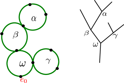
Figure 1.

We say that $S$ is stable if for the associated tree the valency of each vertex is at least 3.

To make some arguments and notation cleaner, we also introduce a linear ordering on the smooth components of $S$, or vertices, by “order of operation” defined as follows. The component with the root semi-infinite edge $e_{0}$ will be called the root vertex denoted by $\omega$. In terms of the associated tree for the surface we have a pre-order on vertices given by the distance to the root vertex, (by giving each edge length 1). To get an actual order, first isometrically embed the tree in the plane, while preserving the clockwise ordering of each half-infinite edge, corresponding to the ordering of the punctures. Then clockwise order vertices equidistant to the root, as in Figure 1. We shall denote by ${\alpha}$ the furthermost component from $\omega$, i.e. it is the greatest element with respect to our order. Then ${\beta}$ is the next furthermost component, etc. (Pretending that we can’t run out of letters.) Note, that $\alpha$ may not be the leftmost component, in fact “leftmost” may be ambiguous (dependent on the embedding) for vertices not equidistant to $\omega$.

Remark 3.2.

This correspondence of letters to the order may seem counterintuitive, but this is motivated by idea that these trees are operadic trees determining composition. More explicitly, later on this is the composition in certain $A_{\infty}$ Fukaya categories. Composition corresponding to furthermost elements from $\omega$ is performed first. Hence $\alpha$ corresponds to the first operation we need to perform. Although the operations corresponding to components equidistant from $\omega$ can be performed in any order.

As part of the data, we may ask for a holomorphic diffeomorphism at each $i$’th end, having the name of the end:

$$e_{i}:[0,1]\times(0,\infty)\to S,$$

$i\neq 0$. And at the 0’th puncture we ask for a holomorphic diffeomorphism

$$e_{0}:[0,1]\times(-\infty,0)\to S.$$

These charts will be called strip end charts.

When $S^{\prime}$ is not nodal, these strip end charts have the property that

$$S-ends:=S-\cup_{i\in\{0,\ldots,d\}}\operatorname{image}(e_{i})$$

is a compact surface with corners.

Let $S_{j,\pm}^{\circ},S_{j,\pm}$ be as above. We further specify the $\pm$ distinction so that $S_{j,-}>S_{j,+}$ with respect to the linear order above. And we may ask for a similar pair of strip charts

(3.2) $$e_{j,-}:[0,1]\times(-\infty,0)\to S^{\circ}_{j,-},$$

(3.3) $$e_{j,+}:[0,1]\times(0,\infty)\to S^{\circ}_{j,+}$$

at the $n_{j,{\pm}}$ ends. The data of all such strip charts for a given $S$, will be called a a strip end structure.

The moduli space of the Riemann surfaces as above, with $\operatorname{Card}I=d$, will be denoted by $\overline{\mathcal{R}}_{d}$. (Note that Seidel [23] calls our $\overline{\mathcal{R}}_{d}$ by $\overline{\mathcal{R}}_{d+1}$.) $\overline{\mathcal{R}}_{d}$ is a real dimension $d-2$ manifold with corners. We will also denote by $\mathcal{R}_{d}\subset\overline{\mathcal{R}}$ the subspace corresponding to non-nodal surfaces.

For $d\geq 2$ let $\rho^{\prime}:{\mathcal{S}}_{d}\to\overline{\mathcal{R}}_{d}$ denote the universal family of the Riemann surfaces $S$, as above. Denote by

$$\rho:{\mathcal{S}}^{\circ}_{d}\to\overline{\mathcal{R}}_{d},$$

this universal family where the nodal points of the surface fibers have been removed.

Notation 3.3.

We denote by $\mathcal{S}_{d,r}$ and sometimes just by $\mathcal{S}_{r}$ the fiber $\rho^{-1}(r)$, for $r\in\overline{\mathcal{R}}_{d}$.

Choose $r$-smooth (varying smoothly with respect to $r$) families $\{e_{i,r}\}$, $\{e_{j,\pm,r}\}$ of strip end structures for the entire universal family ${\mathcal{S}}_{d}\to\overline{\mathcal{R}}_{d}$, (note that further on $r$ is suppressed). These choices have to be consistent with gluing in the natural sense as explained in [23, Section 9g]. We will keep track of these systems of choices of strip end structures only implicitly.

3.2.1. Metric characterization of the moduli space

It will be helpful to recall the characterization of the moduli space ${\mathcal{R}}_{d}$ and its compactification $\overline{\mathcal{R}}_{d}$, in terms of hyperbolic metrics on the punctured disks $S_{r}$. The family $\{{\mathcal{S}}_{d,r}\}_{r\in{\mathcal{R}}_{d}}$ is in a bijective correspondence with a suitably universal family $\{\mathcal{M}et_{r}\}=\{\mathcal{M}et_{d,r}\}$ of constant curvature $-1$ metrics on the disk with $d+1$ punctures on the boundary. Under this correspondence the complex structure on $\mathcal{S}_{r}$ is just the conformal structure induced by $\mathcal{M}et_{r}$. This is of course classical, to see all this use Schwartz reflection to “double” each $\mathcal{S}_{r}$ to a connected genus 0 Riemann surface $\mathcal{D}_{r}$, without boundary. This determines an embedding of ${\mathcal{R}}_{d}$ into the moduli space ${M}_{0,d+1}$ of Riemann surfaces that are topologically $S^{2}$ with $d+1$ points removed. As $d>2$, by the uniformization theorem, each $\mathcal{D}_{r}$ is a quotient of the disk by a subgroup of $PSL(2,\mathbb{R})$, which must also preserve the hyperbolic metric. Therefore, $\mathcal{S}_{r}$ inherits a hyperbolic metric, that we call $Met_{r}$.

The metric point of view gives an illuminating description of the compactification $\overline{\mathcal{R}}_{d}$, for $d\geq 2$. Starting with some $\mathcal{S}_{r}$ and taking $r$ to a boundary stratum, corresponds to some fixed collection of embedded, disjoint geodesics on $\mathcal{S}_{r}$, with boundary in the boundary of $\mathcal{S}_{r}$, have their length shrunk to zero. Each boundary stratum of $\overline{\mathcal{R}}_{d}$ is completely determined by such a collection of geodesics.

3.2.2. Gluing

The gluing construction (see for example [23]) takes a surface $\mathcal{S}_{r}$, $r\in\partial\overline{\mathcal{R}}_{d}$ and produces a surface with one less node. This gluing is determined by gluing parameters which we parametrize by $[0,1)$, assigned to each node. For us $0$ means don’t glue, and 1 is meant to correspond to some small value of the gluing parameter used in actual gluing. We will write $d_{\alpha,\beta}$ for the parameter used in the gluing of components $\alpha,\beta$, and likewise with other components.

The gluing construction for parameters in $[0,1)$ determines an open neighborhood called gluing neighborhood of the boundary of $\overline{\mathcal{R}}_{d}$. A gluing normal neighborhood of the boundary of $\overline{\mathcal{R}}_{d}$: will be an open neighborhood (usually denoted $N$) of the boundary, deformation retracting to the boundary, contained in the gluing neighborhood.

The gluing construction also induces a kind of thick-thin decomposition of the surface, with thin parts conformally identified with $[0,1]\times(0,l)$ for $l>0$ determined by the corresponding gluing parameter. This decomposition is not intrinsic, as it depends in particular on the choice of the family of strip end structures. However, instructively these gluing parameters can be thought of as lengths of geodesic segments, for example $m_{\alpha}$, $m_{\beta}$ in figure 2, and the thin parts are closely related to thin parts of thick-thin decomposition in hyperbolic geometry.

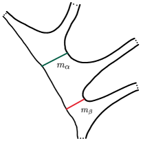
Figure 2. This diagram is only schematic. The embedding into the plane is not meant to be holomorphic or isometric for the natural hyperbolic structure on the surface.

3.3. Hamiltonian fibrations

A Hamiltonian fibration is a smooth fiber bundle

$$M\hookrightarrow P\to X,$$

with structure group $\mathcal{G}=\text{Ham}(M,\omega)$ with its $C^{\infty}$ Frechet topology. A Hamiltonian connection, in this paper usually denoted by caligraphic letters of the kind $\mathcal{A}$, is just an Ehresmann $\mathcal{G}$-invariant connection for a Hamiltonian fibration. When $P=M\times X$ is trivial, such $\mathcal{A}$ may be specified as a one form valued in $C^{\infty}_{norm}(M)$ - the space of smooth functions on $M$ with mean 0.

4. A system of natural maps from the universal curve to $\Delta^{n}$

We explain here a remarkable connection between the universal curve over $\overline{\mathcal{R}}_{d}$ and the standard topological simplices $\Delta^{n}$. This will be used in our construction but may be of independent interest.

Let $\Pi(\Delta^{n})$ be the small groupoid, whose objects set $obj$ is the set of vertices of $\Delta^{n}$. The morphisms set $hom$ is the set of affine maps $m:[0,1]\to\Delta^{n}$, (possibly constant) sending end points to the vertices. The source map

$$s:hom\to obj$$

is defined by $s(m)=m(0)$ and the target map

$$t:hom\to obj$$

is defined by $t(m)=m(1)$. Thus, the set $hom(v_{1},v_{2})$ of morphisms between $v_{1},v_{2}\in\Pi(\Delta^{n})$ consists of a single morphism. It is the unique affine map $m:[0,1]\to\Delta^{n}$, satisfying $m(0)=v_{1}$ and $m(1)=v_{2}$. Consequently, the composition maps in $\Pi(\Delta^{n})$ are forced, by the above uniqueness. And the identity at $v$ is the constant $m:[0,1]\to\Delta^{n}$, $m(0)=m(1)=v$.

Notation 4.1.

We denote the composition of $m_{1},m_{2}$ by $m_{1}\cdot m_{2}$. The order is diagrammatic, so that this means the composition

$$\cdot\xrightarrow{m_{1}}\cdot\xrightarrow{m_{2}}\cdot.$$

We say that $(m_{1},\ldots,m_{d})$ is a composable chain of morphisms $m_{i}\in hom(\Pi(\Delta^{n}))$ if $t(m_{i-1})=s(m_{i})$, for all $2\leq i\leq d$ . For future use let $m_{i-1,i}$ denote the unique morphism from the $i-1$ vertex to the $i$ vertex in $\Delta^{n}$.

The goal is to construct a “natural” system of maps

$${u}(m_{1},\ldots,m_{d},n):{\mathcal{S}}^{\circ}_{d}\to\Delta^{n},$$

$d\geq 2$, for each composable chain $(m_{1},\ldots,m_{d})$. To give a preview, the reason why we work with $\mathcal{S}^{\circ}_{d}$ instead of $\mathcal{S}_{d}$, is that certain naturality conditions that we impose, force that the node ends (images of charts $e_{j,\pm}$ ) of the surface map to an edge of $\Delta^{n}$. Given continuity, this is of course impossible if the edge is non-constant, unless the node itself is removed.

Let us order the boundary components $0,\ldots,d$ of a surface $\mathcal{S}_{r}$, $r\in\mathcal{R}_{d}$, as follows. The ordering is clockwise with 0 the component on the left of the $e_{0}$ end, given that we have chosen the embedding with $e_{0}$ pointing downward. See Figure 3.

Figure 3.

Definition 4.2.

We say that ${u}(m_{1},\ldots,m_{d},n):{\mathcal{S}}^{\circ}_{d}\to\Delta^{n}$ satisfies partial naturality if the following holds.

1. The map ${u}(m_{1},\ldots,m_{d},n)$ is continuous and its restriction to

   $$\rho^{-1}(\mathcal{R}_{d}\subset\overline{\mathcal{R}}_{d})$$

   is smooth.

2. Let ${u}(m_{1},\ldots,m_{d},n,r)$ denote the restriction of ${u}(m_{1},\ldots,m_{d},n)$ to $\mathcal{S}_{r}$, and let

   $$m_{0}:=m_{1}\cdot\ldots\cdot m_{d}$$

   be the composition in $\Pi(\Delta^{n})$. Then given the strip end charts $e_{k}:[0,1]\times(0,\infty)\to\mathcal{S}_{r}$ at each $e_{k}$ end, $1\leq k\leq d$,

   $$e_{k}\circ{u}(m_{1},\ldots,m_{d},n,r)=m_{k}\circ pr$$

   for $pr:[0,1]\times(0,\infty)\to[0,1]$ the projection.

3. Likewise, in the strip end coordinates $e_{k}:[0,1]\times(-\infty,0)\to\mathcal{S}_{r}$ at the end $e_{0}$ of $\mathcal{S}_{r}$, ${u}(m_{1},\ldots,m_{d},n,r)$ has the form of the projection to $[0,1]$ composed with $m_{0}$.

4. For $0\leq k\leq d-1$, $r\in\mathcal{R}_{d}$, the $k$’th component of $\partial\mathcal{S}_{r}$ is mapped to $s(m_{k})$, and the $d$’th component is mapped by ${u}(m_{1},\ldots,m_{d},n,r)$ to $t(m_{d})$.

See Figure 4 for an example of a map satisfying partial naturality.

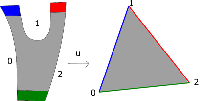
Figure 4. Figure for a map $u(m_{0,1},m_{1,2},2)$ satisfying partial naturality. The edges of the surface labeled $0,1,2$ are mapped to the vertices $0,1,2$ respectively. Colored ends are collapsed onto correspondingly colored edges.

So far we haven’t put any special conditions for $r\in\partial\overline{\mathcal{R}}_{d}$, having to do with nodes. These conditions will be forced by certain additional naturality axioms, which arise from various gluing conditions. After imposing these additional axioms, Theorems 4.8, 4.12 which will follow, state that such a natural system of maps exists and is unique up to suitable concordance.

We start by explaining the natural gluing operations that appear.

Notation 4.3.

In what follows we may interchangeably use the notation $\mathcal{S}^{\circ}(d),\mathcal{S}(d)$ for $\mathcal{S}^{\circ}_{d},\mathcal{S}_{d}$. This is to avoid notation clash with various notations for fibers.

First denote by $\mathcal{T}(m_{1},\ldots,m_{d},n)$ the space of maps satisfying the partial naturality properties above. We have the natural gluing map

(4.1) $$St_{i}:\overline{\mathcal{R}}_{s_{1}}\times\overline{\mathcal{R}}_{s_{2}}\times[0,1)\to\overline{\mathcal{R}}_{s_{1}+s_{2}-1},$$

whose value on $(r,r^{\prime},\tau)$ is given by gluing the surfaces $\mathcal{S}_{r},\mathcal{S}_{r^{\prime}}$ at the root of $\mathcal{S}_{r}$ and at the $i$’th marked point of $\mathcal{S}_{r^{\prime}}$, with gluing parameter $\tau\in[0,1)$, and then associating to this glued surface its isomorphism class in $\overline{\mathcal{R}}_{s_{1}+s_{2}-1}$. (When the value of the gluing parameter is 0, this is the composition map in the Stasheff topological $A_{\infty}$ operad).

Given an element $u\in\mathcal{T}(m_{1},\ldots,m_{s_{1}},n)$ and an element

$$u^{\prime}\in\mathcal{T}(m^{\prime}_{1},\ldots,m^{\prime}_{i-1},m_{1}\cdot\ldots\cdot m_{s_{1}}=m^{\prime}_{i},m^{\prime}_{i+1},\ldots,m^{\prime}_{s_{2}},n),$$

we have a naturally induced map

$$(u\star_{i}u^{\prime})_{0}:{\mathcal{S}}^{\circ}({s_{1},s_{2},0})\to\Delta^{n},$$

where

$${\mathcal{S}}^{\circ}({s_{1},s_{2},0})\to\overline{\mathcal{R}}_{s_{1}}\times\overline{\mathcal{R}}_{s_{2}}$$

is the pullback of the fibration

$${\mathcal{S}}^{\circ}({d=s_{1}+s_{2}-1})\to\overline{\mathcal{R}}_{s_{1}+s_{2}-1}$$

by $St_{i}|_{\overline{\mathcal{R}}_{s_{1}}\times\overline{\mathcal{R}}_{s_{2}}\times\{0\}}$. More specifically, the fiber $\mathcal{S}_{r_{1},r_{2}}$ of ${\mathcal{S}}^{\circ}({s_{1},s_{2},0})$ over $(r_{1},r_{2})$ is the disjoint union of a pair of distinguished (possibly disconnected) subspaces ${S}_{1},{S}_{2}$ naturally identified with $\mathcal{S}_{r_{1}}(s_{1})$, respectively $\mathcal{S}_{r_{2}}(s_{2})$. So under this identification, we apply $u$ to ${S}_{1}$ and $u^{\prime}$ to ${S}_{2}$, and this is the map $(u\star_{i}u^{\prime})_{0}|_{\mathcal{S}_{r_{1},r_{2}}}$, see Figure 5.

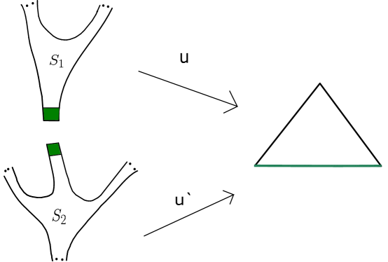
Figure 5. The green shaded ends are collapsed onto the same edge of $\Delta^{n}$.

We can extend $(u\star_{i}u^{\prime})_{0}$ to a map

$$(u\star_{i}u^{\prime})_{1}:{\mathcal{S}}^{\circ}({s_{1},s_{2},1})\to\Delta^{n},$$

where

$${\mathcal{S}}^{\circ}({s_{1},s_{2},1})\to\overline{\mathcal{R}}_{s_{1}}\times\overline{\mathcal{R}}_{s_{2}}\times[0,1)$$

is the pullback of the family

$${\mathcal{S}}^{\circ}({d=s_{1}+s_{2}-1})\to\overline{\mathcal{R}}_{s_{1}+s_{2}-1}$$

by $St_{i}|_{\overline{\mathcal{R}}_{s_{1}}\times\overline{\mathcal{R}}_{s_{2}}\times[0,1)}$.

To get this extension we specify

(4.2) $$(u\star_{i}u^{\prime})_{r,r^{\prime},\tau}:=(u\star_{i}u^{\prime})_{1}|_{\mathcal{S}_{r,r^{\prime},\tau}},$$

for $\mathcal{S}_{r,r^{\prime},\tau}$ the fiber of ${\mathcal{S}}^{\circ}({s_{1},s_{2},1})$ over

$$(r,r^{\prime},\tau)\in\overline{\mathcal{R}}_{s_{1}}\times\overline{\mathcal{R}}_{s_{2}}\times[0,1),\quad\tau\in(0,1).$$

Recall that the surface $\mathcal{S}_{r,r^{\prime},\tau}$ glued from $\mathcal{S}_{r},\mathcal{S}_{r^{\prime}}$ has a subdomain which we denote by $thin=thin_{\tau,i}$ that has a determined conformal identification with a strip of the form $[0,1]\times(-\phi(\tau),\phi(\tau))$, for some continuous function (not explicitly needed)

(4.3) $$\phi:(0,1]\to(0,\infty),$$

s.t. $\lim_{\tau\mapsto 0}\phi(\tau)=\infty$. This function is determined by the particular parametrization of the gluing operation.

Now $\mathcal{S}_{r,r^{\prime}}-thin$ is the disjoint union of subspaces holomorphically identified with the regions

$$Reg_{r}\subset\mathcal{S}_{r},Reg_{r^{\prime}}\subset\mathcal{S}_{r^{\prime}},$$

so that $Reg_{r}$ is identified with $\mathcal{S}_{r}-\operatorname{image}{e_{0}}$, where $e_{0}$ is the strip end chart for the root end of $\mathcal{S}_{r}$. And likewise, so that $Reg_{r^{\prime}}$ is identified $\mathcal{S}_{r^{\prime}}-\operatorname{image}e_{i}$, for $e_{i}$ the strip end chart for the $i$’th end of $\mathcal{S}_{r^{\prime}}$.

We then define $(u\star_{i}u^{\prime})_{r,r^{\prime},\tau}$ to coincide with $u$, $u^{\prime}$ on $Reg_{r}$ respectively $Reg_{r^{\prime}}$, while on $thin$ in the distinguished coordinates

$$[0,1]\times(-\phi(\tau),\phi(\tau)),$$

$(u\star_{i}u^{\prime})_{r,r^{\prime},\tau}$ is the map given by the projection

$$[0,1]\times(-\phi(\tau),\phi(\tau))\to[0,1]$$

followed by the map $m^{\prime}_{i}$, similarly to the Axiom 2 of partial naturality. This operation is well-defined for all $\tau\in(0,1)$ and so determines the needed extension.

In order to state the naturality axioms we need more geometry. Let $N$ be a gluing normal neighborhood of the boundary $\partial\overline{\mathcal{R}}_{d}$, $d\geq 3$. Recall that $\mathcal{R}_{d}$ has dimension $d-2$. Let $S^{d-3}_{0}\subset N$ be an embedded sphere of dimension $d-3$, not intersecting $\partial\overline{\mathcal{R}}_{d}$, homotopic to the inclusion $(\partial\overline{\mathcal{R}}_{d}\simeq S^{d-3})\to N$. (A $0$-dimensional sphere is understood throughout as a pair of points.) Let $R^{d-2}_{0}$ be the dimension $d-2$ ball subdomain of $\overline{\mathcal{R}}_{d}$ bounded by $S^{d-3}_{0}$. Finally, let $\mathcal{S}_{r}-ends$ denote the compact Riemann surface with boundary obtained from $\mathcal{S}_{r}$ by removing the ends. Specifically, for $1\leq i\leq d$ we remove the images of the charts $e_{i}:{[0,1]\times(0,\infty)}\to\mathcal{S}_{r}$, and we remove the image of the chart $e_{0}:[0,1]\times(-\infty,0)\to\mathcal{S}_{r}$.

For $r\notin\partial\overline{\mathcal{R}}_{d}$ set $D^{2}_{r}:=\mathcal{S}_{r}-ends\simeq D^{2}$. And let

$$G^{2}_{r}:=(D^{2}_{r},\partial D^{2}_{r})\simeq(D^{2},\partial D^{2})$$

denote the pair, where $\simeq$ is homeomorphism.

So we get a fiber bundle of pairs

$$(D^{2},\partial D^{2})\hookrightarrow(\widetilde{F},A)\to R^{d-2}_{0},$$

with fiber over $r$: $G^{2}_{r}$. And where $A$ is just the corresponding sub-bundle with fiber over $r$: $\partial D^{2}_{r}$.

We are almost ready to state our axioms. Let $C_{s}(\Delta^{n})$ denote the set of composable chains $(m_{1},\ldots,m_{s})$ of length $s\geq 2$ in $\Pi(\Delta^{n})$.

Definition 4.4.

For $(m_{1},\cdots,m_{s})\in C_{s}(\Delta^{n})$ let $D(m_{1},\ldots,m_{s})$ denote the minimal dimension of a subsimplex of $\Delta^{n}$ which contains the edges corresponding to the morphisms $m_{i}$.

A system of maps $\mathcal{U}$ is an element of:

(4.4) $$\prod_{n\in\mathbb{N}}\prod_{s\in\mathbb{N}_{\geq 2}}\prod_{(m_{1},\ldots,m_{s})\in C_{s}(\Delta^{n})}\mathcal{T}(m_{1},\ldots m_{s},n).$$

Given a system $\mathcal{U}$ its projection onto $(n,s,(m_{1},\ldots,m_{s}))$ component will be denoted by $u(m_{1},\ldots,m_{s},n)$. To put this another way, let

$$B=\{(m_{1},\ldots m_{s},n)|s\in\mathbb{N}_{\geq 2},n\in\mathbb{N},(m_{1},\ldots,m_{s})\in C_{s}(\Delta^{n})\},$$

then set theoretically the product (4.4) above is the set of certain set maps $\mathcal{U}$ with domain $B$. Then in this language $u(m_{1},\ldots,m_{s},n)=\mathcal{U}(m_{1},\ldots,m_{s},n).$

Definition 4.5.

We say that $\mathcal{U}$ is natural if it satisfies the following axioms:

1. For all $s_{1},s_{2}$ and for all $i$ if $m_{i}^{\prime}=m_{1}\cdot\ldots\cdot m_{s_{1}}$ then the map

   (4.5) $$({u}(m_{1},\ldots,m_{s_{1}},n)\star_{i}u(m^{\prime}_{1},\ldots,m^{\prime}_{s_{2}},n))_{1}$$

   coincides with the composition

   (4.6) $${\mathcal{S}}^{\circ}_{s_{1},s_{2},1}\xrightarrow{St_{i,*}}{\mathcal{S}}_{s_{1}+s_{2}-1}^{\circ}\xrightarrow{u(m^{\prime}_{1},\ldots,m^{\prime}_{i-1},m_{1},\ldots,m_{s_{1}},m_{i+1},\ldots,m^{\prime}_{s_{2}},n)}\Delta^{n},$$

   for $St_{i,*}$ the bundle map induced by $St_{i}$. ($St_{i,*}$ is the natural map in the corresponding pull-back square.)

2. Let $f:\Delta^{n}\to\Delta^{m}$ be a simplicial map, which recall is an affine map preserving the orders of the vertices. Then there is an induced functor

   $$f:\Pi(\Delta^{n})\to\Pi(\Delta^{m})$$

   and we ask that

   $$f\circ u(m_{1},\ldots,m_{s},n)=u(f(m_{1}),\ldots,f(m_{s}),m).$$

3. Let $(m_{1},\ldots,m_{d})\in C_{d}(\Delta^{d})$ for $d\geq 3$. Suppose that $D(m_{1},\ldots,m_{d})=d$ then by the Lemma 4.7 below, $u(m_{1},\ldots,m_{d},d)$ induces a map of pairs:

   (4.7) $$\widetilde{u}:(\widetilde{F},A\sqcup\widetilde{F}|_{S_{0}^{d-3}})\to(\Delta^{d},\partial\Delta^{d}),$$

   and we ask that $\widetilde{u}$ be a homological degree 1 map.

Remark 4.6.

Note that when $d=2$ we may still state an analogue of Axiom 3, but it would be immediate from the partial naturality properties of Definition 4.2.

Lemma 4.7.

Let $\mathcal{U}$ satisfy the first pair of axioms in the Definition 4.5. For $(m_{1},\cdots,m_{d})\in C_{s}(\Delta^{d})$, $d\geq 3$, suppose that $D(m_{1},\ldots,m_{d})=d$. Then $\widetilde{u}:=u(m_{1},\ldots,m_{d},d)$ is a map of pairs:

$$\widetilde{u}:(\widetilde{F},A\sqcup\widetilde{F}|_{S_{0}^{d-3}})\to(\Delta^{d},\partial\Delta^{d}).$$

Proof.

The map $\widetilde{u}$ maps $A$ to $\partial\Delta^{d}$ by the partial naturality properties 2,3 and 4 in Definition 4.2. In fact $A$ is mapped to the edges of $\Delta^{d}$.

Since $S_{0}^{d-3}$ is contained $N$, by Axiom 1 for each $r\in S_{0}^{d-3}$, ${u}_{r}=u(m_{1},\ldots,m_{d},n,r)$ has the form $(u_{1}\star_{i}u_{2})_{\tau,r_{1},r_{2}}$ for some $i$, for some

$$u_{1}\in\mathcal{T}(m_{1},\ldots,m_{s_{1}},d)$$

for some

$$u_{2}\in\mathcal{T}(m^{\prime}_{1},\ldots,m^{\prime}_{i-1},m_{1}\cdot\ldots\cdot m_{s_{1}}=m^{\prime}_{i},m^{\prime}_{i+1},\ldots,m^{\prime}_{s_{2}},d),$$

and some $\tau,r_{1},r_{2}$.

Now $s_{1}<d$ and $s_{2}<d$ since $s_{1}+s_{2}-1=d$, and since $s_{1},s_{2}\geq 2$. It then follows by this and by Axiom 2 that the images of $u_{1}$ and $u_{2}$ are contained in proper faces of $\Delta^{d}$. Consequently, the image of $\widetilde{u}|_{S_{0}^{d-3}}$ is contained in $\partial\Delta^{d}$ and so we are done. ∎

Theorem 4.8.

A natural system $\mathcal{U}$ exists.

We first give a not explicitly constructive proof in all generality, and afterwards describe a partial explicit construction.

Proof of 4.8.

To construct our maps $u(m_{1},\ldots,m_{s},n)$ we will proceed by induction. When $n=0$ there is nothing to do, as we have unique maps for all $s\geq 2$, and they trivially satisfy Axioms 1,2,3. However, we will have to be careful with the basis of the induction.

Given a composable sequence $(m_{1},\ldots,m_{s})$ of morphisms in $\Pi(\Delta^{n})$, for some $n$, let $D(m_{1},\ldots,m_{s})$, called the $D$-number, denote the least dimension of a non-degenerate subsimplex of $\Delta^{n}$ that contains the edges corresponding to $\{m_{i}\}$. Let $S(N)$ be the following statement: there are maps

(4.8) $$u(m_{1},\ldots,m_{s},n),$$

for all $s\geq 2$ and all $n\leq N$ and every composable chain $(m_{1},\ldots,m_{s})$ with $D(m_{1},\ldots,m_{s})=s\leq n$ such that axioms 1,3 are satisfied and such that

(4.9) $$\sigma\circ u(m_{1},\ldots,m_{s},n)=u(\sigma(m_{1}),\ldots,\sigma(m_{s}),n)$$

for

$$\sigma:\Delta^{n}\to\Delta^{m}$$

an injective simplicial map. That is we satisfy Axiom 2 only partially and only for restricted $(m_{1},\ldots,m_{s})$ at the moment.

We will also denote by $S(N)$ a corresponding collection of maps (4.8) with the requisite property. It can be seen directly that $S(N)$ holds for $N=0,1,2,3$. $N=0$ is the trivial case already considered above. Indeed, when $N=4$ such a construction is given in the following Section 4.2, and this also implies the cases of $N=1,2,3$. We intend to prove:

$$(N\geq 3)\land S(N)\implies S(N+1),$$

moreover the collection of maps $S(N+1)$ can be chosen to extend the collection of maps $S(N)$.

Note that the condition 4.9 and the maps (4.8) uniquely determine

(4.10) $$u(m_{1},\ldots,m_{s},N+1)$$

for $\forall s\geq 2,\forall(m_{1},\ldots,m_{s})$ with $D(m_{1},\ldots,m_{s})=s\leq N$. We need an extension in the case $D(m_{1},\ldots,m_{s})=s=N+1$.

By assumption $N+1>3$. Let then $(m^{0}_{1},\ldots,m_{N+1}^{0})$, be a chosen composable sequence with $D(m^{0}_{1},\ldots,m^{0}_{N+1})=N+1$. Then gluing as in the Axiom 1 of naturality and the maps (4.10) naturally determine a map

(4.11) $${u}={u}(m^{0}_{1},\ldots,m^{0}_{N+1},N+1):Sub_{N+1}\to\Delta^{N+1},$$

where $Sub_{N+1}=\rho^{-1}(\partial\overline{\mathcal{R}}_{N+1})$, and where as before

$$\rho:{\mathcal{S}}_{N+1}^{\circ}\to\overline{\mathcal{R}}_{N+1}.$$

Let $U$ be a gluing normal neighborhood of $\mathcal{R}_{N+1}$. (We previously used the letter $N$, but just for this proof we use the letter $U$.) Extend ${u}$ in any way to $\rho^{-1}(U)$, so that Axiom 1 of naturality is satisfied. We then need to further extend ${u}$ to ${\mathcal{S}}_{N+1}^{\circ}$ so that Axiom 3 of naturality is satisfied.

Let $S^{N-2}_{0}\subset U$ be an embedded sphere in $U$ not intersecting $\partial\overline{\mathcal{R}}_{N+1}$, homotopic to the inclusion $\partial\overline{\mathcal{R}}_{N+1}\to U$. Then $u$ induces a map of a pair

(4.12) $$g:(\widetilde{F}|_{S_{0}^{N-2}},A|_{S_{0}^{N-2}})\to(\partial\Delta^{N+1}\simeq S^{N},loop),$$

where $loop$ is a topologically embedded $S^{1}$ in $\partial\Delta^{N+1}$ that is the image of the loop

$$\gamma=m^{0}_{1}\cdot\ldots\cdot m^{0}_{N+1}\cdot m_{s(m^{0}_{1}),t(m^{0}_{N+1})}^{-1},$$

where $\cdot$ is concatenation of paths and the order of composition is diagrammatic. The map $g$ is just the restriction of the map $\widetilde{u}$, (4.7).

Lemma 4.9.

The map $g$ is homological degree 1.

Proof.

As $N>2$ $loop$ has codimension greater than 1, so that the meaning of homological degree is unambiguous, as the pair $(S^{N},loop)$ has a well-defined fundamental class by the homology long exact sequence for a pair. Moreover, approximating $g$ by a smooth map we may compute the homological degree via the smooth degree, (denote the approximation still by $g$). That is let $f$ be a $N$-face of $\Delta^{N+1}$ and $p\in interior(f)$ a regular image point of $g$. The homological degree of $g$ is then the count of elements of $g^{-1}(p)$ with signs given by whether $dg_{k}$, $k\in g^{-1}(p)$, is orientation preserving or reversing.

Suppose without loss of generality that the vertices of $f$ are $0,\ldots,N$. As the degree of $g$ is clearly independent of the choice of $S_{0}^{N-2}$ we may assume that $S_{0}^{N-2}$ is chosen so that for some $\epsilon>0$:

(4.13) $$St_{1}:\left(R_{0}^{N-2}\subset\overline{\mathcal{R}}_{N}\right)\times\overline{\mathcal{R}}_{2}\times\{\epsilon\}\to\overline{\mathcal{R}}_{N+1}$$

is an embedding into $S_{0}^{N-2}$. Note that the map

$$St_{1}:\left(R_{0}^{N-2}\subset\overline{\mathcal{R}}_{N}\right)\times\overline{\mathcal{R}}_{2}\times\{0\}\to\overline{\mathcal{R}}_{N+1}$$

may be understood as a “face map” for the polyhedral model of $\mathcal{R}_{N+1}$. We may in addition suppose that $S_{0}^{N-2}-T$ is covered by such embeddings corresponding to the various other “faces” of $\overline{\mathcal{R}}_{N+1}$, where the region $T\subset S_{0}^{N-2}$, is such that $g$ maps $\rho^{-1}(T)$ into the union of $(N-1)$-faces of $\Delta^{N+1}$. The image of the map (4.13) will be denoted by $V$.

Then by the naturality Axiom 3 the face $f$ is covered by the image of

$$\kappa=({u}(m^{0}_{1},\ldots,m^{0}_{N},N+1)\star_{1}u(m^{0}_{1}\cdot\ldots\cdot m^{0}_{N},m^{0}_{N+1},N+1))_{1}|_{\widetilde{V}},$$

where

$$\widetilde{V}=\rho^{-1}(V).$$

By construction, the smooth degree of $g|_{\widetilde{V}}$ is the smooth degree of $\kappa$. But then, by the naturality Axiom 3, $\kappa$ has smooth degree one. And again, by naturality and the assumption on the form of $S_{0}^{N-2}$, as described above, no other point of $\widetilde{F}|_{S_{0}^{N-2}}$ is in $g^{-1}(p)$. It follows that $g$ is smooth degree one and so is homological degree one.

∎

Lemma 4.10.

There is a degree one extension:

$$\widetilde{g}:(\widetilde{F},A\sqcup\widetilde{F}|_{S_{0}^{N-2}})\to(\Delta^{N+1},\partial\Delta^{N+1}),$$

with $\widetilde{g}(A)=loop$.

Proof.

This is elementary topology so that we will not give exhaustive detail. Note that $\widetilde{F}\simeq B^{N-1}\times D^{2}$, where $B^{N-1}$ denotes the unit ball in $\mathbb{R}^{N-1}$. So to find the necessary degree one extension it is enough to show that given a degree one map $h:(S^{d-2}\times D^{2},S^{d-2}\times\partial D^{2})\to(S^{d},loop)$, there is a degree one extension

$$\widetilde{h}:(B^{d-1}\times D^{2},\partial B^{d-1}\times D^{2})\to(B^{d+1},\partial B^{d+1}).$$

First note that a degree one map

$$\widetilde{t}:(B^{d-1}\times D^{2},\partial B^{d-1}\times D^{2})\to(B^{d+1},\partial B^{d+1}),$$

exists by an elementary topology construction. (Start with the slicing diffeomorphism $[0,1]^{d-1}\times[0,1]^{2}\to[0,1]^{d+1}$.) We may in addition ensure that the restriction of $\widetilde{t}$ to the boundary $S^{d-2}\times D^{2}$ is a map of a pair

$$t:(S^{d-2}\times D^{2},S^{d-2}\times\partial D^{2})\to(S^{d},loop).$$

We may now apply an analogue of the classical theorem of Hopf, which says that homotopy classes of maps of closed $d$-manifolds to $S^{d}$ are classified by degree. (We say analogue because we are working with maps of pairs.) In our case Hopf’s theorem readily implies that $t$ is homotopic to $h$ through maps of pairs. Then use classical homotopy extension theorem, to get a homotopy from $\widetilde{t}$ to the needed map $\widetilde{h}$, extending $h$. ∎

Continuing with the proof of the theorem, given $\widetilde{g}$ as in the lemma above, we may readily construct our extension $u:{\mathcal{S}}_{N+1}^{\circ}\to\Delta^{N+1}$ so that

$$u\in\mathcal{T}(m^{0}_{1},\ldots,m^{0}_{N+1},N+1)$$

and so that the last naturality axiom is satisfied.

Now given any other composable sequence $(m_{1},\ldots,m_{N+1})$ with

$$D(m_{1},\ldots,m_{N+1})=N+1$$

let

$$\sigma:\Delta^{N+1}\to\Delta^{N+1}$$

be the unique simplicial bijective map taking $(m_{1},\ldots,m_{N+1})$ to $(m^{0}_{1},\ldots,m^{0}_{N+1})$, (it is unique because the action is determined by the action on the vertices. ) And we define

$$u(m_{1},\ldots,m_{N+1},N+1):{\mathcal{S}}_{N+1}^{\circ}\to\Delta^{N+1}$$

by

$$u(m_{1},\ldots,m_{N+1},N+1)=\sigma^{-1}\circ u.$$

We then obtain a collection of maps,

$$\{u(m_{1},\ldots,m_{s^{\prime}},n)\}_{(m_{1},\ldots,m_{s^{\prime}}),n\leq N+1,D(m_{1},\ldots,m_{s^{\prime}})=s^{\prime}\leq n},$$

and these maps satisfy the condition of the statement $S(N+1)$ by the construction and the inductive hypothesis. We thus complete the inductive step. Moreover, by construction the collection of maps $S(N+1)$ extends the collection $S(N)$.

By recursion, we may then define a sequence of systems $\{S_{N}\}_{N\geq 0}$, so that $S(N+1)$ extends $S(N)$, for each $N$. We then obtain the total collection:

$$\mathcal{U}^{\prime}=\bigcup_{N}S(N)=\{u(m_{1},\ldots,m_{s^{\prime}},n)|n\in\mathbb{N},(m_{1},\ldots,m_{s^{\prime}})\in C_{s^{\prime}}(\Delta^{n}),$$

$$\text{ such that }D(m_{1},\ldots,m_{s^{\prime}})=s^{\prime}\}.$$

It remains to extend the partial system $\mathcal{U}^{\prime}$ above to a full natural system $\mathcal{U}$, that is we need to remove restrictions on the $D$-number. Given $(m_{1},\ldots,m_{s})$, a composable sequence in $\Pi(\Delta^{n})$ with $s>n$, we may write $m_{i}=pr\circ\widetilde{m}_{i}$ for $(\widetilde{m}_{1},\ldots,\widetilde{m}_{s})$ a composable sequence in $\Delta^{s}$ s.t. $D(\widetilde{m}_{1},\ldots,\widetilde{m}_{s})=s$, for $pr:\Delta^{s}\to\Delta^{n}$ surjective simplicial map. We then define

$$u(m_{1},\ldots,m_{s},n):=pr\circ u(\widetilde{m}_{1},\ldots,\widetilde{m}_{s},s).$$

We should check that the above is well-defined. Let $(\widetilde{m}^{\prime}_{1},\ldots,\widetilde{m}^{\prime}_{s})$ be another choice of a composable sequence with $pr(\widetilde{m}^{\prime}_{i})=m_{i}$. There is a unique simplicial bijective map $\sigma:\Delta^{s}\to\Delta^{s}$ fixing the image $i(\Delta^{n})$, for $i:\Delta^{n}\to\Delta^{s}$ inclusion of face, s.t. $pr\circ i=id$, and s.t. $\sigma(\widetilde{m}_{i})=\widetilde{m}^{\prime}_{i}$.

Then we have

$$pr\circ u(\widetilde{m}^{\prime}_{1},\ldots,\widetilde{m}^{\prime}_{s},s)=pr\circ\sigma\circ u(\widetilde{m}_{1},\ldots,\widetilde{m}_{s},s).$$

But $pr\circ\sigma=pr$ since $\sigma$ fixes $i(\Delta^{n})$. So we obtain that

$$pr\circ u(\widetilde{m}^{\prime}_{1},\ldots,\widetilde{m}^{\prime}_{s},s)=pr\circ u(\widetilde{m}_{1},\ldots,\widetilde{m}_{s},s),$$

so that $u(m_{1},\ldots,m_{s},n)$ is well-defined. So we have constructed our system of maps satisfying all the axioms of naturality. ∎

4.1. Target dependent natural systems

Our natural systems $\mathcal{U}$ can be made dependent on particular simplices $\Sigma:\Delta^{d}\to X$. This is useful for proving invariance later on. More specifically, for $X$ a smooth manifold, a target dependent system $\mathcal{U}(X)$ is an element of

(4.14) $$\prod_{\Sigma^{n}\in\Delta(X)}\prod_{s\in\mathbb{N}_{\geq 2}}\prod_{(m_{1},\ldots,m_{s})\in C_{s}(\Delta^{n})}\mathcal{T}(m_{1},\ldots m_{s},n),$$

where $\Sigma^{n}$ is a singular $n$-simplex for $n\in\mathbb{N}$. As before given a system $\mathcal{U}(X)$ its projection onto $(\Sigma^{n},s,(m_{1},\ldots,m_{s}))$ component will be denoted by $u(m_{1},\ldots,m_{s},\Sigma^{n})$. The superscript $n$ may be omitted, when the degree $n$ is not explicitly needed.

Definition 4.11.

Similarly to the Definition 4.5, we say that $\mathcal{U}(X)$ is natural if it satisfies the following axioms:

1. For all $\Sigma^{n}$, $s_{1},s_{2}$ and for all $i$ if $m_{i}^{\prime}=m_{1}\cdot\ldots\cdot m_{s_{1}}$ then the map

   (4.15) $$({u}(m_{1},\ldots,m_{s_{1}},\Sigma^{n})\star_{i}u(m^{\prime}_{1},\ldots,m^{\prime}_{s_{2}},\Sigma^{n}))_{1}$$

   coincides with the composition

   (4.16) $${\mathcal{S}}^{\circ}_{s_{1},s_{2},1}\xrightarrow{St_{i,*}}{\mathcal{S}}_{s_{1}+s_{2}-1}^{\circ}\xrightarrow{u(m^{\prime}_{1},\ldots,m^{\prime}_{i-1},m_{1},\ldots,m_{s_{1}},m_{i+1},\ldots,m^{\prime}_{s_{2}},\Sigma^{n})}\Delta^{n},$$

   for $St_{i,*}$ the bundle map induced by $St_{i}$.

2. Let $f:\Sigma^{n}\to\Sigma^{m}$ be a morphism in $\Delta(X)$, then there is an induced functor

   $$f:\Pi(\Delta^{n})\to\Pi(\Delta^{m}),$$

   and we ask that

   $$f\circ u(m_{1},\ldots,m_{s},\Sigma^{n})=u(f(m_{1}),\ldots,f(m_{s}),\Sigma^{m}),$$

   where $f$ on the left is the corresponding map $f:\Delta^{n}\to\Delta^{m}$, cf. (3.1).

3. Let $(m_{1},\ldots,m_{d})\in C_{d}(\Delta^{d})$ for $d\geq 3$. Suppose that $D(m_{1},\ldots,m_{d})=d$. Then, as in Definition 4.5, $u(m_{1},\ldots,m_{d},\Sigma^{d})$ induces a map of pairs:

   (4.17) $$\widetilde{u}:(\widetilde{F},A\sqcup\widetilde{F}|_{S_{0}^{d-3}})\to(\Delta^{d},\partial\Delta^{d}),$$

   and we ask that $\widetilde{u}$ be a homological degree 1 map.

Theorem 4.12.

Given a smooth manifold $X$, a natural $\mathcal{U}(X)$ exists and is unique up to concordance. (We shall say what this means in the proof.)

Proof.

Existence is simple. Pick a natural system $\mathcal{U}$ guaranteed by Theorem 4.8. This induces a target dependent natural system $\mathcal{U}(X)$ defined by:

$$\forall\Sigma^{n}:u(m_{1},\ldots,m_{s},\Sigma^{n})=u(m_{1},\ldots,m_{s},n),$$

where the maps $u(m_{1},\ldots,m_{s},n)$ correspond to $\mathcal{U}$.

Now uniqueness up to concordance means that given a pair $\mathcal{U}_{1}(X),\,\mathcal{U}_{2}(X)$ of natural systems, there is a natural system $\widetilde{\mathcal{U}}(X\times I)$ whose restriction to $X\times\{i\}$ is $\mathcal{U}_{i}(X)$, $i=0,1$. The proof of this is totally analogous to the inductive construction in the proof of Theorem 4.8. ∎

4.2. Outline of an explicit construction

This section is not logically necessary, but in order to give the reader more intuition we now give a partial explicit construction of a natural system $\mathcal{U}$ (not its target dependent analogue). To be more formal, we give an explicit construction of the system satisfying condition $S(4)$, as in the proof of Theorem 4.8. However, we will not check all the properties. (Although this would be straightforward.) This construction could be in principle extended to all generality but at the cost of much complexity.

Fix a geometric model for $\overline{\mathcal{R}}_{d}$, for example as the Stasheff associahedra. When $d=4$ this is a pentagon. Recall that to each corner of $\overline{\mathcal{R}}_{4}$ we have a uniquely associated nodal Riemann surface with 3 components and 5 marked points, one of which is called the root.

Recall that we label the root component by $\omega$, the next component by $\beta$ and the component furthest from root by $\alpha$. (With respect to the linear ordering described earlier.) Denote by $M_{\alpha}$ the collection of marked points, different from the root $e_{0}$, on $\alpha$, likewise with $\beta,\omega$. This determines a sub-composable sequence $mor(S_{\alpha})$ of a composable sequence $(m_{1},\ldots,m_{4})$, and likewise with $\beta,\omega$, (note that $M_{\omega},M_{\beta}$ could be empty).

Let $r$ be in the gluing normal neighborhood of some corner, corresponding to non-zero gluing parameters $d_{\alpha,\beta}$, $d_{\beta,\omega}$. We now construct a map

$$f_{r}=f_{r}(m_{1},\ldots,m_{4}):[0,4]\times[0,1]\to\Delta^{4}.$$

In what follows by concatenation of a collection of paths we mean their product in the Moore path category of $\Delta^{4}$, the notation for composition will be assumed to be diagrammatic. This is the category with objects: points of $\Delta^{4}$, and morphisms from $x_{0}$ to $x_{1}$: continuous paths $[0,T]\to\Delta^{4}$, $T>0$, between $x_{0},x_{1}$, with composition the natural concatenation of paths. Note that this is quite different from our previously defined groupoid $\Pi(\Delta^{4})$.

For a morphism $m$ in $\Pi(\Delta^{4})$ let $s(m)$ and $t({m})$ denote the source respectively target of $m$. Let $H^{m}:\Delta^{4}\times[0,1]\to\Delta^{4}$ denote the natural deformation retraction of $\Delta^{4}$ onto the edge determined by $s(m),t(m)$, with time $1$ map the orthogonal affine projection onto this edge (for the standard metric on $\Delta^{n}$). Set $H^{m}_{\tau}=H^{m}|_{\Delta^{n}\times\{\tau\}}$. Next, for a general piece-wise affine path $p:[0,T]\to\Delta^{4}$, with end points $s(m),t(m)$, we have a homotopy $H^{m}_{\tau}\circ p$, $\tau\in[0,1]$, from $p$ to a path

$$\widetilde{p}:[0,T]\to\Delta^{4}$$

with image in the edge determined by $m$. Let $D(p,\tau)$, $\tau\in[0,1]$, be the concatenation of $H^{m}_{\tau}\circ p$ with the homotopy $G_{\tau}$, $\tau\in[0,1]$, of paths with fixed end points, from $\widetilde{p}$ to the map

$$\widetilde{m}:[0,T]\to\Delta^{4}$$

linearly parametrizing the edge determined by $m$. This second homotopy $G_{\tau}$ can be chosen in a way that depends only on $\widetilde{p}$. This can be done explicitly, using piece-wise linearity of $p$.

The map $f^{t}_{r}$ from the $y=t$ slice $[0,4]\times\{t\}$ is constructed as follows. Set

$$I_{\alpha}=(1-d_{\alpha,\beta})/2,$$

and set $f_{\alpha,r}$ to be the concatenation of the morphisms in $mor(M_{\alpha})$. That is if

$$M_{\alpha}=(m^{\alpha}_{1},\ldots,m^{\alpha}_{k})$$

then

$$f_{\alpha,{r}}=m^{\alpha}_{1}\cdot\ldots\cdot m^{\alpha}_{k}.$$

Then for $t\in[0,I_{\alpha}]$ set $f^{t}_{\alpha,r}=D(f_{\alpha,r},2t)$. Then set $f^{t}_{r}$ to be the concatenation of morphisms in $mor(M_{\beta})$, $mor(M_{\gamma})$ and of $f^{t}_{\alpha,r}$, in that order, although note that the order of the morphisms in the concatenation is uniquely determined by the end point conditions, this holds further on as well.

Next set

$$I_{\beta}=I_{\alpha}+(1-I_{\alpha})(1-d_{\beta})/2.$$

If $\alpha$ and $\beta$ components have a nodal point in common we set

$$f_{\beta,r}:[0,4]\times\{t\}\to\Delta^{4}$$

to be the concatenation of $f^{I_{\alpha}}_{\alpha,r}$ with morphisms in $mor(M_{\beta})$, and for $t\in[I_{\alpha},I_{\beta}]$ we set

$$f^{t}_{\beta,r}=D(f_{\beta,r},{\frac{2(t-I_{\alpha})}{1-I_{\alpha}}}).$$

And then for $t\in[I_{\alpha},I_{\beta}]$ set $f^{t}_{r}$ to be the concatenation of morphisms in $mor(M_{\omega})$ and of $f^{t}_{\beta,r}$.

Finally, set $f_{\omega,r}$ to be the concatenation of $f^{I_{\beta}}_{\beta,r}$ with morphisms in $mor(M_{\omega})$, and for $t\in[I_{\beta},1]$ set

$${f}^{t}_{r}=D({f_{\omega,r}},\frac{2(t-I_{\beta})}{1-I_{\beta}}).$$

When $\alpha$ has a nodal point in common with the $\omega$ component set $f_{\beta,r}$ to be the concatenation of morphisms in $mor(M_{\beta})$, and for $t\in[I_{\alpha},I_{\beta}]$ set

$$f^{t}_{\beta,r}=D({f_{\beta,r}},{\frac{2(t-I_{\alpha})}{1-I_{\alpha}}}).$$

Then for $t\in[I_{\alpha},I_{\beta}]$ set $f^{t}_{r}$ to be the concatenation of morphisms $f^{I_{\alpha}}_{r}$ and $f^{t}_{\beta,r}$, and $mor(M_{\omega})$ (although $mor(M_{\omega})$ in this particular case is empty, we add this so that the degenerate case $M_{\alpha}=\emptyset$, $M_{\beta}=\emptyset$ makes sense, see the discussion below). Finally, for $t\in[I_{\beta},1]$ set

$$f^{t}_{r}=D({f_{r}^{I_{\beta}}},{\frac{2(t-I_{\beta})}{1-I_{\beta}}}).$$

When $r\in\overline{\mathcal{R}}_{4}$ is in the gluing neighborhood of a face but not of a corner the construction of $f_{r}:[0,4]\times[0,1]\to\Delta^{4}$ is similar, in fact we can think of it as a special case of the above by setting $d_{\beta}=1$, $M_{\beta}=\emptyset$. When $r\in\overline{\mathcal{R}}_{4}$ is not in the gluing neighborhood of the boundary we can also think of this as a special case of the above, with $M_{\alpha}=\emptyset,M_{\beta}=\emptyset$, $d_{\alpha}=1$, $d_{\beta}=1$ in the construction above.

4.2.1. Retracting $\mathcal{S}_{r}$ onto $[0,4]\times[0,1]$

We now construct a smooth $r$-family of maps

$$ret_{r}:{\mathcal{S}}_{r}\to[0,4]\times[0,1],$$

$r\in{\mathcal{R}}_{4}$, suitably compatible with the maps

$${f}_{r}:[0,4]\times[0,1]\to\Delta^{4}.$$

In figure 6 $(a)$, $(b)$, $(c)$ represent cases where $(c)$: $r$ is not within gluing normal neighborhood of boundary, $(b)$: $r$ is in a gluing neighborhood of a side but not a corner and $(a)$: $r$ is within gluing neighborhood of a corner, (we picked a particular corner and side for these diagrams). The color shading will be explained in a moment. In each case $(a),(b),(c)$ we first color shade $[0,4]\times[0,1]$ as in figure 7, the green region is the domain of $f^{t}_{\alpha,r}$ contained in $[0,4]\times[0,I_{\alpha}]$, in the blue regions the map $f_{r}$ is vertically constant, the red region is the domain of $f^{t}_{\beta,r}$ contained in $[0,4]\times[I_{\alpha},I_{\beta}]$ and yellow region is the rest of the domain of $f_{r}$. The maps $ret_{r}$ are defined for each $r$ by taking color shaded areas to color shaded areas, so that the following holds.

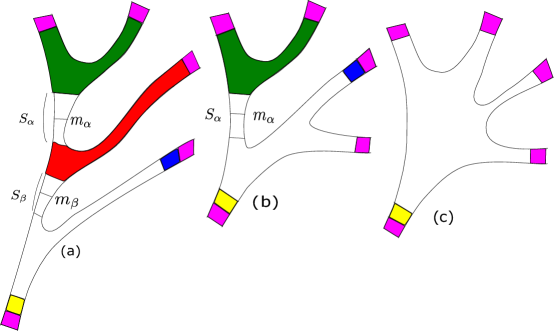
Figure 6. The uncolored enclosed regions labeled $S_{\alpha}$, $S_{\beta}$ surrounding segments $m_{\alpha}$, $m_{\beta}$ are “thin”.

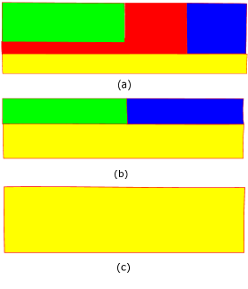
Figure 7. Diagram for $S_{d}$. Solid black border is boundary, while dashed red lines are open ends. The connection $\mathcal{A}({r,\{L_{i}\}})$ preserves Lagrangians $L_{i}$ over boundary components labeled $L_{i}$.

1. The ends $e_{i}$, $i=1,\ldots,4$ of $\mathcal{S}_{r}$, colored in purple, are identified in strip end coordinates as $(0,\infty)\times[0,1]$ and in these coordinates $ret_{r}$ is the composition of the projection $(0,\infty)\times[0,1]\to[0,1]$, with the map $\underline{m}_{i}$ to the boundary of $[0,4]\times[0,1]$, characterized as follows: $f_{r}\circ\underline{m}_{i}$ parametrizes the morphism $m_{i}\in\Pi(\Delta^{4})$. Similarly for the $e_{0}$ end.

2. The boundary of $\mathcal{S}_{r}$ goes either to the boundary of $[0,4]\times[0,1]$ or to the vertical boundary lines between colored regions.

3. The unshaded “thin” regions labeled $S_{\alpha}$, $S_{\beta}$ come from the gluing construction and are identified with $[0,1]\times(-\phi(\tau_{\alpha}),\phi(\tau_{\alpha}))$, respectively $[0,1]\times(-\phi(\tau_{\beta}),\phi(\tau_{\beta}))$. In these coordinates $ret_{r}$ on $S_{\alpha}$, $S_{\beta}$ is the projection to $[0,1]$ composed with a diffeomorphism onto the lower edge of the green, respectively the red region, (affine in respective natural coordinates).

4. The unshaded part of $\mathcal{S}_{r}$ is collapsed onto the horizontal line bounding yellow region of $[0,4]\times[0,1]$.

5. Blue shaded regions are identified in strip end coordinates $(0,\infty)\times[0,1]\to\Sigma_{r}$, as $[0,1]\times[0,1]$, and are mapped to the corresponding blue regions in $[0,4]\times[0,1]$.

(The above prescription naturally extends to the boundary $\overline{\mathcal{R}}_{4}$.)

We then set

$$u(m_{1},\ldots,m_{4},\Delta^{4})|_{\mathcal{S}_{r}}=f_{r}\circ ret_{r}.$$

These are almost the maps we want, but we need to “collar them” near the boundary of $\overline{\mathcal{R}}_{4}$, so that Axiom 1 of naturality is satisfied. We omit the details.

5. Auxiliary data $\mathcal{D}$

Let

$$M\hookrightarrow P\xrightarrow{\pi}X$$

be a Hamiltonian fiber bundle, with model fiber $(M,\omega)$ that we shall assume here to be a closed, monotone:

$$[\omega]=const\cdot 2c_{1}(TM),$$

$const>0$, symplectic manifold. The constant $const$ is called the monotonicity constant.

We now discuss geometric-analysis theoretic data needed for the construction of the functor $F_{P}:\Delta(X)\to A_{\infty}-Cat^{unit}$, as outlined in Section 1.1 of the introduction. Essentially, this data $\mathcal{D}=\mathcal{D}(P)$ specifies a choice of a (target dependent) natural system $\mathcal{U}$ and various choices of Hamiltonian connections, as well as certain choices of almost complex structures. These choices are to be made for each $\Sigma\in Simp(X)$, while being suitably compatible, so that we obtain our functor $F_{P}$.

For $(M,\omega)$ as above, we say that a Lagrangian submanifold $L\subset M$ is monotone if the homomorphisms given by symplectic area and Maslov class

$$[\omega]:H_{2}(M,L)\to\mathbb{R},\quad\mu:H_{2}(M,L)\to\mathbb{Z}$$

are proportional:

$$[\omega]=const\cdot\mu.$$

For an $x:pt\to X$, define

(5.1) $$F(x)=F_{P}(x),$$

to be the set of oriented, spin, monotone Lagrangian submanifold $L$ in

$$(P_{x}=x^{*}P,\omega_{x})\simeq(M,\omega)$$

with minimal (positive) Maslov number at least 2, and such that the inclusion map $\pi_{1}(L)\to\pi_{1}(M)$ vanishes. We call elements of $F_{P}(x)$ objects. These will in fact be objects of a certain $A_{\infty}$ category to be constructed.

Let $L\in F_{P}(x)$, and $j$ be an almost complex structure on $P_{x}$ tamed by $\omega_{x}$, meaning that

$$\forall v\in TP_{x},v\neq 0:\omega_{x}(v,jv)>0.$$

Let $\mathcal{M}(L,j)$ denote the moduli space of Maslov number 2 $j$-holomorphic discs in $P_{x}$, with one marked point on the boundary, with boundary of the disk in $L$. It is well known, see Sheridan [24, Section 2.3] (which also contains a number of additional references) that for a generic such $j$, $\mathcal{M}(L,j)$ is regular, is a transversely cut out $n$-dimensional manifold and is compact. The compactness is due to the following fact. If $\mathcal{M}(L,j)$ were not compact, then by Gromov compactness there would be a sequence of curves in

$$\mathcal{M}(L,j)$$

degenerating to a nodal curve with at least a pair of components. One of these components has Maslov number at least $2$, by our assumption on the minimal Maslov number. And the other component contributes positively to the total Maslov number of the nodal curve. (The monotonicity, and energy positivity preclude negative Maslov/Chern number components.) This would clearly be a contradiction, by the additivity of the Maslov number.

Then we have a map corresponding to the evaluation at the marked point:

$$ev:\mathcal{M}(L,j)\to L,$$

and we define $\omega(L)\in\mathbb{Z}$ as the degree of $ev$.

Given a smooth

$$\Sigma:\Delta^{n}\to X,$$

set $x_{i}:=\Sigma(i)\in X$, $i\in\{0,\ldots,n\}$ a vertex of $\Delta^{n}$. Also denote by $x_{i}$ the corresponding inclusion map $x_{i}:pt\to X$. Set

(5.2) $$F_{P}(\Sigma):=\bigsqcup_{i}F_{P}(x_{i}),$$

with elements likewise called objects, at the moment this is just a set of Lagrangians, but later on this will be the set of objects of a certain $A_{\infty}$ category, (with the same name).

Given a pair of objects

$$L_{0},L_{1}\in F_{P}(\Sigma),$$

satisfying

$$\omega(L_{0})=\omega(L_{1}),$$

and such that $L_{0}\in F_{P}(x_{i}),L_{1}\in F_{P}(x_{j}),$ let

$$m=m_{L_{0},L_{1}}:[0,1]\to\Delta^{n}$$

denote the edge between $i,j$ corners of $\Delta^{n}$, $i,j\in\{0,\ldots,n\}$. We then set

$$\overline{m}:=\Sigma\circ m.$$

For each such $\Sigma$, and for each $L_{0},L_{1}$ as above, the data $\mathcal{D}$ prescribes a Hamiltonian connection

$$\mathcal{A}(L_{0},L_{1})=\mathcal{A}(L_{0},L_{1},\overline{m})$$

on $\overline{m}^{*}P$. (See Section 3.3 for definition of Hamiltonian connections.)

Denote by $\mathcal{A}(L_{0},L_{1})(L_{0})$ the Lagrangian $\phi(L_{0})\subset P_{x_{j}}$, for $\phi$ the $\mathcal{A}(L_{0},L_{1})$-parallel transport map over $[0,1]$. Then we require that $\mathcal{A}(L_{0},L_{1})(L_{0})$ be transverse to $L_{1}$.

Definition 5.1.

Let

$$S(L_{0},L_{1})=S(L_{0},L_{1},\mathcal{A}(L_{0},L_{1}))$$

denote the space of $\mathcal{A}({L_{0},L_{1}})$-flat sections with boundary on $L_{0},L_{1}$, over $0$ respectively over $1$. In other words elements of $S(L_{0},L_{1})$ are sections

$$\gamma:[0,1]\to\overline{m}_{L_{0},L_{1}}^{*}P,$$

tangent to the $\mathcal{A}(L_{0},L_{1})$-horizontal distribution and satisfying $\gamma(0)\in L_{0}$ and $\gamma(1)\in L_{1}$. By a starting position of an element $\gamma\in S(L_{0},L_{1})$ we mean $\gamma(0)\in L_{0}$. Likewise by an ending position of an element $\gamma\in S(L_{0},L_{1})$ we mean $\gamma(1)\in L_{1}$.

Definition 5.2.

Let $m=m_{L_{0},L_{1}}$ be as above, and let

$$\{j_{t}\}_{t\in[0,1]}=j(L_{0},L_{1},\overline{m})$$

be a family of fiber-wise almost complex structures on $\overline{m}^{*}P$, s.t. for each $t$ $j_{t}$ is tamed by the symplectic form $\omega_{\overline{m}(t)}$ on $P_{\overline{m}(t)}$. Then $\{j_{t}\}$ is said to be admissible with respect to $\mathcal{A}(L_{0},L_{1})$ if the following holds.

• For each $t$, Chern number $1$ $j_{t}$-holomorphic spheres in $P_{\overline{m}(t)}\subset\overline{m}^{*}P$ do not intersect any of the images of any elements of $S(L_{0},L_{1})$.

• The moduli spaces $\mathcal{M}(L_{0},j_{0})$, $\mathcal{M}(L_{1},j_{1})$ are regular, and the evaluation map

  $$ev_{0}:\mathcal{M}(L_{0},j_{0})\to L_{0}$$

  does not intersect the set of starting positions of elements of $S(L_{0},L_{1})$. Likewise, the evaluation map

  $$ev_{1}:\mathcal{M}(L_{1},j_{1})\to L_{1}$$

  does not intersect the set of ending positions of elements of $S(L_{0},L_{1})$.

Such a family $j(L_{0},L_{1},\overline{m})$ is easily seen to exist, see Sheridan [24]. Our data $\mathcal{D}$ then fixes a choice of such $j(L_{0},L_{1},\overline{m})$ for each $\Sigma,m,L_{0},L_{1}$ as above.

Next $\mathcal{D}$ makes a choice of a target dependent natural system $\mathcal{U}(X)$. Finally, $\mathcal{D}$ will specify a certain natural system of Hamiltonian connections and a system of complex structures that we now describe. This is to be done for all choices of certain Lagrangian labels. This involves some necessarily complicated notation, but there is nothing deep going on, once we have the geometric input of the system $\mathcal{U}(X)$. Loosely speaking, $\mathcal{D}$ is just a system of compatible perturbations in the sense of Sheridan and Seidel but relative to $\mathcal{U}(X)$.

5.1. From a Hamiltonian fibration over $X$ to Hamiltonian fibrations over surfaces

Let $M\hookrightarrow P\to X$ be as before, and let a natural system $\mathcal{U}(X)$ be chosen. Given a composable chain $(m_{1},\ldots,m_{d})$ and a map

$$u(m_{1},\ldots,m_{d},\Sigma^{n}):{\mathcal{S}}_{d}^{\circ}\to\Delta^{n}\text{ that is part of a natural system $\mathcal{U}(X)$},$$

we have an induced fibration

$$M\hookrightarrow\widetilde{S}(m_{1},\ldots,m_{d},\Sigma^{n})\to{\mathcal{S}}_{d}^{\circ}$$

by pulling back $M\hookrightarrow P\to X$ first by $\Sigma^{n}:\Delta^{n}\to X$ and then by $u(m_{1},\ldots,m_{d},\Sigma^{n})$. We have a natural projection

$$\widetilde{S}(m_{1},\ldots,m_{d},\Sigma^{n})\to\overline{\mathcal{R}}_{d},$$

and we denote the fiber over $r\in\overline{{\mathcal{R}}}_{d}$ by $\widetilde{S}(m_{1},\ldots,m_{d},\Sigma^{n},r)$, or simply by $\widetilde{\mathcal{S}}_{r}$ where there can be no confusion. So $\widetilde{\mathcal{S}}_{r}$ is naturally a Hamiltonian $M$-fibration over the surface $\mathcal{S}_{r}$, smooth over smooth components. To state this another way,

$$\widetilde{\mathcal{S}}_{r}=(u(m_{1},\ldots,m_{d},\Sigma^{n},r)\circ\Sigma)^{*}P,$$

where

(5.3) $$u(m_{1},\ldots,m_{d},\Sigma^{n},r):=u(m_{1},\ldots,m_{d},\Sigma^{n})|_{\mathcal{S}_{r}}.$$

5.1.1. Distinguished trivializations

By the partial naturality properties of the maps $u(m_{1},\ldots,m_{d},\Sigma^{n},r)$, at each $e_{i}$ end, $1\leq i\leq d$, of $\mathcal{S}_{r}$, we have natural trivializations

$$(0,\infty)\times\overline{m}_{i}^{*}P\to\widetilde{\mathcal{S}}_{r}.$$

Similarly, at the $e_{0}$ and. For $r\in\mathcal{R}_{d}$, we also have natural trivializations of $\widetilde{\mathcal{S}}_{r}$ over the $i$’th boundary component of $\mathcal{S}_{r}$, $0\leq i\leq d-1$, as $\mathbb{R}\times P_{s(m_{i+1})}$. Or as $\mathbb{R}\times P_{t(m_{d})}$ over $d$’th boundary component. The ordering is as described in the preamble of Section 4, see also Figure 3. There are analogous natural trivializations also for general $r\in\overline{\mathcal{R}}_{d}$. We shall call these distinguished trivializations/coordinates. And the structure of these trivializations will be called the distinguished trivialization structure.

5.2. Lagrangian labels and admissible connections

Given $r\in\mathcal{R}_{d}$, and given choices

$$L_{i}\in F(\overline{m}_{i+1}(0)),\text{ for $0\leq i\leq d-1$, }\quad L_{d}\in F(\overline{m}_{d}(1)),$$

such that $\omega(L_{i})=\omega(L_{d})$ for all $i=0,\ldots,d$, a labeling is just an assignment of $L_{i}$ to the $i$’th component of $\partial\mathcal{S}_{r}$. Extend the labeling construction above naturally to $\mathcal{S}_{r}$, with $r\in\partial\overline{\mathcal{R}}_{d}$. In other words, for such an $\mathcal{S}_{r}$, we label the boundary components in such a way that if we glue at some node of $\mathcal{S}_{r}$ then each boundary component of the glued surface inherits a consistent label. See Figure 8 below.

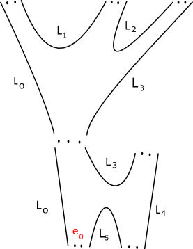
Figure 8.

For the moment we do not specify any dependence of the labels on $r$.

Let us from now on omit the superscript $n$ in $\Sigma^{n}$ where there is no need to disambiguate.

Definition 5.3.

We say that a Hamiltonian connection (cf. Section 3.3) $\mathcal{A}$ on the Hamiltonian fibration

$$M\hookrightarrow\widetilde{\mathcal{S}}(m_{1},\ldots,m_{d},\Sigma,r)\to\mathcal{S}_{r},$$

$r\in\overline{\mathcal{R}}_{d}$, is admissible with respect to a labeling $L_{0},\ldots,L_{d}$ if:

• Parallel transport by $\mathcal{A}$ over the boundary component(s) of $\partial\mathcal{S}_{r}$ labeled $L_{i}$ preserves the Lagrangian $L_{i}$, $0\leq i\leq d$, in the distinguished coordinates.

• For $1\leq i\leq d$, in the distinguished coordinates $(0,\infty)\times\overline{m}_{i}^{*}P$, at each $e_{i}$ end,

  $$\mathcal{A}=\widetilde{\mathcal{A}}(L_{i-1},L_{i},\overline{m}_{i}):=pr^{*}\mathcal{A}(L_{i-1},L_{i},\overline{m}_{i})$$

  for

  $$pr:(0,\infty)\times\overline{m}_{i}^{*}P\to\overline{m}_{i}^{*}P$$

  the natural bundle map projection. Here $\mathcal{A}(L_{i-1},L_{i},\overline{m}_{i})$ are part of our data $\mathcal{D}$ as previously discussed.

• Likewise, at the $e_{0}$ end in the distinguished coordinates $(-\infty,0)\times\overline{m}_{0}^{*}P$, $\mathcal{A}=pr^{*}\mathcal{A}(L_{0},L_{d},\overline{m}_{0})$ for $pr$ similarly defined.

We do not yet impose any conditions at the nodes, but certain conditions will be forced by the additional properties of the Definition 5.6 below. For a preview, we remark that $\mathcal{D}$ will make a choice of such a connection for all possible $L_{0},\ldots,L_{d}$ as above.

We also have a Lagrangian sub-fibration of

$$\widetilde{\mathcal{S}}_{r}\to\mathcal{S}_{r}$$

over the boundary of $\mathcal{S}_{r}$, whose fiber over an element of the boundary component labeled $L_{i}$ is $L_{i}$, in the distinguished coordinates. (This naturally extends to the case $\mathcal{S}_{r}$ is nodal.)

We name this sub-fibration by

(5.4) $${\mathcal{L}}(\mathcal{U},L_{0},\ldots,L_{d},r).$$

In particular, by construction, if $\mathcal{A}$ is admissible with respect to $L_{0},\ldots,L_{d}$ as above then it preserves this sub-fibration.

Notation 5.4.

Denote by

$$\mathcal{T}(m_{1},\ldots,m_{d};L_{0},\ldots,L_{d},\Sigma,r)=\mathcal{T}(L_{0},\ldots,L_{d},\Sigma,r)$$

the space of Hamiltonian connections on

$$M\hookrightarrow\widetilde{\mathcal{S}}(m_{1},\ldots,m_{d},\Sigma,r)\to\mathcal{S}_{r}$$

admissible with respect to $L_{0},\ldots,L_{d}$. Note that this implicitly requires a chosen system $\mathcal{U}(X)$, which will not be indicated.

5.3. Gluing admissible connections.

Given an element

$$\mathcal{A}\in\mathcal{T}(m_{1},\ldots,m_{s_{1}};L_{0},\ldots,L_{s_{1}},\Sigma,r)$$

and an element

$$\mathcal{A}^{\prime}\in\mathcal{T}(m_{1},\ldots,m_{s_{2}};L^{\prime}_{0},\ldots,L^{\prime}_{i-1},L^{\prime}_{i},L^{\prime}_{i+1},\ldots,L^{\prime}_{s_{2}},\Sigma,r^{\prime}),$$

s.t. $m_{1}\cdot\ldots\cdot m_{s_{1}}=m^{\prime}_{i}$ and s.t. $L^{\prime}_{i-1}=L_{0},L^{\prime}_{i}=L_{s_{1}}$, we have a naturally induced glued connection $(\mathcal{A}\star_{i}\mathcal{A}^{\prime})_{\tau}$ on

$$\widetilde{\mathcal{S}}_{r,r^{\prime},\tau}:=(u\star_{i}u^{\prime})_{r,r^{\prime},\tau}^{*}\circ\Sigma^{*}P,$$

where $(u\star_{i}u^{\prime})_{r,r^{\prime},\tau}$ is as in (4.2). The construction of the connection $(\mathcal{A}\star_{i}\mathcal{A}^{\prime})_{\tau}$ is analogous to the construction of the maps $(u\star_{i}u^{\prime})_{r,r^{\prime},\tau}$, see also Figure 9.

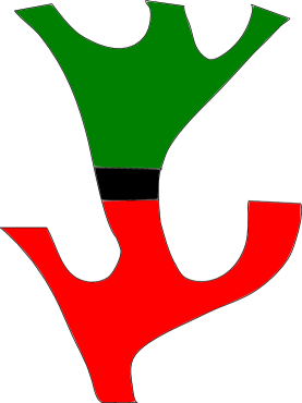
Figure 9. The green region is identified with a subregion of the surface $\mathcal{S}_{r}$, the red region is identified with a subregion of the surface $\mathcal{S}_{r^{\prime}}$. We have similar identifications of the fibration $\widetilde{\mathcal{S}}_{r,r^{\prime},\tau}$ over these regions with (sub-fibrations of) of $\widetilde{\mathcal{S}}_{r},\widetilde{\mathcal{S}}_{r^{\prime}}$. Then with respect to this identification $(\mathcal{A}\star_{i}\mathcal{A}^{\prime})_{\tau}$ over the green region is the connection $\mathcal{A}$, and over the red region it is the connection $\mathcal{A}^{\prime}$. Over the black region $(\mathcal{A}\star_{i}\mathcal{A}^{\prime})_{\tau}$ is the connection $pr^{*}\mathcal{A}(L_{i-1},L_{i},\overline{m}^{\prime}_{i})$, discussed ahead.

The pair $\mathcal{A},\mathcal{A}^{\prime}$ as above will be called composable. Thus, applying Axiom 1 of naturality of $\mathcal{U}(X)$, for a composable pair $\mathcal{A},\mathcal{A}^{\prime}$ as above we get induced connections $\{St_{i}(\mathcal{A},\mathcal{A}^{\prime},\tau)\}_{0\leq\tau<1}$, so that

$$St_{i}(\mathcal{A},\mathcal{A}^{\prime},\tau)\in\mathcal{T}(L^{\prime}_{0},\ldots,L^{\prime}_{i-2},L_{0},\ldots,L_{s_{1}},L^{\prime}_{i+2},\ldots,L^{\prime}_{s_{2}},\Sigma,St_{i}(r,r^{\prime},\tau)),$$

for $0\leq\tau<1$, and so that in addition we have the following.

Over the thin region $thin_{\tau,i}\subset\mathcal{S}_{St_{i}(r,r^{\prime},\tau)}$, for $\tau>0$, $\widetilde{\mathcal{S}}_{St_{i}(r,r^{\prime},\tau)}$ is naturally isomorphic to the fibration

$$(-\phi(\tau),\phi(\tau))\times(\overline{m}^{\prime}_{i})^{*}P\to(-\phi(\tau),\phi(\tau))\times[0,1]$$

by Axiom 2, 3 of partial naturality, and Axiom 1 naturality. Here $\phi$ is as in (4.3). We likewise call this isomorphism the distinguished coordinates/representation extending the previous use of this term. Then over $thin_{\tau,i}$, in the above distinguished representation, $St_{i}(\mathcal{A},\mathcal{A}^{\prime},\tau)$ is the connection $pr^{*}\mathcal{A}(L_{i-1},L_{i},\overline{m}^{\prime}_{i})$, where

$$pr:(-\phi(\tau),\phi(\tau))\times(\overline{m}^{\prime}_{i})^{*}P\to(\overline{m}^{\prime}_{i})^{*}P$$

is the natural projection.

5.4. Admissible fiber almost complex structures

Definition 5.5.

We say that a family $\{j_{z}\}$ of fiber-wise, $\{\omega_{z}\}$-compatible, almost complex structures on the Hamiltonian $M$-fibration $\widetilde{\mathcal{S}}(m_{1},\ldots,m_{d},\Sigma,r)\to\mathcal{S}_{r}$ is admissible with respect to $L_{0},\ldots,L_{d}$ if:

• At the $i$’th end of $\mathcal{S}_{r}$, $1\leq i\leq d$ in the distinguished trivialization

  $$(0,\infty)\times\overline{m}_{i}^{*}P\to\widetilde{\mathcal{S}}$$

  we have

  $$\{j_{z}\}=\widetilde{j}(L_{i-1},L_{i}):=pr^{*}j(L_{i-1},L_{i},\overline{m}_{i})$$

  for

  $$pr:(0,\infty)\times\overline{m}_{i}^{*}P\to\overline{m}_{i}^{*}P$$

  the projection. Here ${j}(L_{i-1},L_{i},\overline{m}_{i})$, is as in Definition 5.2, and is part of our data $\mathcal{D}$ as previously discussed.

• At the $e_{0}$ end, define admissibility analogously.

5.5. Gluing admissible fiber almost complex structures

Denote by

$$\mathcal{J}(L_{0},\ldots,L_{s},\Sigma,r)$$

the space of families of fiberwise almost complex structures $\{j_{z}\}$ on

$$\widetilde{\mathcal{S}}(m_{1},\ldots,m_{s},\Sigma,r)$$

admissible with respect to $L_{0},\ldots,L_{s}$.

Given an element $\{j_{z}\}$ in $\mathcal{J}(L_{0},\ldots,L_{s_{1}},\Sigma,r)$ and an element

$$\{{j}^{\prime}_{z}\}\in\mathcal{J}(L^{\prime}_{0},\ldots,L^{\prime}_{i-2},L_{0},L_{s_{1}},L^{\prime}_{i+1},\ldots,L^{\prime}_{s_{2}},\Sigma,r^{\prime}),$$

the pair $\{j_{z}\},\{j^{\prime}_{z}\}$ will be called composable. For such a composable pair, analogously to the definition of $St_{i}(\mathcal{A},\mathcal{A}^{\prime},\tau)$, we have an induced element:

$$St_{i}(\{j_{z}\},\{j^{\prime}_{z}\},\tau)\in\mathcal{J}(L^{\prime}_{0},\ldots,L^{\prime}_{i-2},L_{0},\ldots,L_{s_{1}},L^{\prime}_{i+2},\ldots,L^{\prime}_{s_{2}},\Sigma,St_{i}(r,r^{\prime},\tau)),$$

for each $0\leq\tau<1$.

5.6. Combining admissible connections and fiber almost complex structures

Definition 5.6.

Let $M\hookrightarrow P\to X$ be as above. A system $\mathcal{F}=\mathcal{F}(P)$ of connections, and almost complex structures relative to a system $\mathcal{U}(X)$ is an element of

$$\prod_{\Sigma\in Simp(X)}\prod_{s\geq 2}\prod_{\{(L_{0},\ldots,L_{s})|L_{i}\in F(\Sigma)\}}\prod_{r\in\overline{\mathcal{R}}_{s}}\mathcal{T}(L_{0},\ldots,L_{s},\Sigma,r)\times\mathcal{J}(L_{0},\ldots,L_{s},\Sigma,r),$$

(the system $\mathcal{U}(X)$ is implicit in the above.) The projection of $\mathcal{F}$ onto the $(\Sigma,s,(L_{0},\ldots,L_{s}),r)$ component will be denoted by $\mathcal{F}(L_{0},\ldots,L_{s},\Sigma,r)$. To phrase this in functional language, let

$$O=\{(L_{0},\ldots L_{s},\Sigma,r)|s\in\mathbb{N}_{\geq 2},\Sigma\in Simp(X),$$

$$L_{i}\in F(\Sigma),r\in\overline{\mathcal{R}}_{s}\},$$

then set theoretically the product above is the set of certain maps $\mathcal{F}$ with domain $O$. Then in this language $\mathcal{F}(L_{0},\ldots,L_{s},n,r)$ is just the value $\mathcal{F}(L_{0},\ldots,L_{s},n,r),$ of the map $\mathcal{F}$.

Let $pr_{i}$, $i=1,2$, denote the projections

$$pr_{1}:\mathcal{T}(L_{0},\ldots,L_{s},\Sigma,r)\times\mathcal{J}(L_{0},\ldots,L_{s},\Sigma,r)\to\mathcal{T}(L_{0},\ldots,L_{s},\Sigma,r)$$

$$pr_{2}:\mathcal{T}(L_{0},\ldots,L_{s},\Sigma,r)\times\mathcal{J}(L_{0},\ldots,L_{s},\Sigma,r)\to\mathcal{J}(L_{0},\ldots,L_{s},\Sigma,r).$$

For shorthand, in what follows, we say that a Hamiltonian connection $\mathcal{A}\in\mathcal{F}$ if it is of the form $pr_{1}\mathcal{F}(L_{0},\ldots,L_{s},\Sigma,r)$, for some $(L_{0},\ldots,L_{s},\Sigma,r)$.

Definition 5.7.

We say that $\mathcal{F}$, relative to a natural $\mathcal{U}(X)$, is natural if:

1. The families of connections/almost complex structures are smooth in the parameter $r$, over smooth components of the surfaces $\mathcal{S}_{r}$. (At the nodes the behavior will be characterized the Axioms 2, 3, below.)

2. For a composable pair $\mathcal{A},\mathcal{A}^{\prime}\in\mathcal{F}$ as above the connection $St_{i}(\mathcal{A},\mathcal{A}^{\prime},0)$ coincides with

   $$pr_{1}\mathcal{F}(L^{\prime}_{0},\ldots,L^{\prime}_{i-2},L_{0},\ldots,L_{s_{1}},L^{\prime}_{i+1},\ldots,L^{\prime}_{s_{2}},\Sigma,St_{i}(r,r^{\prime},0)).$$

3. The pair of connections,

   $$St_{i}(\mathcal{A},\mathcal{A}^{\prime},\tau),$$

   $$pr_{1}\mathcal{F}(L^{\prime}_{0},\ldots,L^{\prime}_{i-2},L_{0},\ldots,L_{s_{1}},L^{\prime}_{i+1},\ldots,L^{\prime}_{s_{2}},\Sigma,St_{i}(r,r^{\prime},\tau)),$$

   also agree for all $0<\tau<1$ on the “thin region” $thin_{\tau,i}$ of $\mathcal{S}_{St_{i}(r,r^{\prime},\tau)}$.

4. Given a morphism in $Simp(X)$, $f:\Sigma_{1}^{n}\to\Sigma_{2}^{m}$, by Axiom 2 of naturality of $\mathcal{U}(X)$, the Hamiltonian bundle $\widetilde{\mathcal{S}}(m_{1},\ldots,m_{d},\Sigma^{n}_{1},r)$ is expressed as a certain pull-back of $\widetilde{\mathcal{S}}(f(m_{1}),\ldots,f(m_{d}),\Sigma_{2}^{m},r)$, where $f$ on the right denotes the corresponding simplicial map $f:\Delta^{n}\to\Delta^{m}$. So that there is a natural bundle map of Hamiltonian $M$-fibrations

   $$p:\widetilde{\mathcal{S}}(m_{1},\ldots,m_{d},\Sigma_{1}^{n},r)\to\widetilde{\mathcal{S}}(f(m_{1}),\ldots,f(m_{d}),\Sigma_{2}^{m},r),$$

   preserving the distinguished trivalization structure. Then we ask that

   $$p^{*}pr_{1}\mathcal{F}(L_{0},\ldots,L_{d},\Sigma_{2}^{m},r)=pr_{1}\mathcal{F}(L_{0},\ldots,L_{d},\Sigma^{n}_{1},r).$$

5. There are analogous conditions on the families of almost complex structures $pr_{2}\mathcal{F}(L_{0},\ldots,L_{s},\Sigma,r)$ that we will not state.

Notation 5.8.

We will sometimes write by abuse of notation $\mathcal{F}(\ldots)$, for either the connection $pr_{1}\mathcal{F}(\ldots)$, or the family of almost complex structures $pr_{2}\mathcal{F}(\ldots)$, since there usually can be no confusion.

Theorem 5.9.

A natural system $\mathcal{F}$ relative to any given natural system $\mathcal{U}(X)$ exists.

Proof.

Restricting to a single $\Sigma:\Delta^{0}\to X$ this is the classical Fukaya category case, and the proof of existence of a natural system is given in Seidel [23, Section 9i] in the language of what Seidel calls compatible system of perturbations, which is completely analogous to the language of connections used here. Although in Seidel’s book only the case of exact Lagrangians in exact symplectic manifolds is considered, this readily extends to our context, since we are not yet concerned with compactness or regularity properties.

In what follows, as usual, we write $\Sigma^{n}$ for a degree $n$ element of $Simp(X)$, i.e. of the form $\Sigma^{n}:\Delta^{n}\to X$. We proceed by induction. Let $S(N)$ be the statement: there is an element

$$\mathcal{F}^{N}\in\prod_{r\in\overline{\mathcal{R}}_{s}}\prod_{\{(L_{0},\ldots,L_{s})|L_{i}\in F(\Sigma^{n})\}}\prod_{s\geq 2}\prod_{\{\Sigma^{n}|n\leq N\}}\mathcal{T}(L_{0},\ldots,L_{s},\Sigma^{n},r)\times\mathcal{J}(L_{0},\ldots,L_{s},\Sigma^{n},r)$$

satisfying naturality condition of Definition 5.7, where the fourth axiom is only required to hold on $Simp^{N}(X)$, the latter denoting the subcategory of simplices of degree up to $N$. $S(N)$ will also denote the corresponding system $\mathcal{F}^{N}$.

$S(0)$ is already explained above. We prove

$$S(N)\implies S(N+1),$$

in addition the corresponding system $S(N+1)$ can be assumed to extend $S(N)$.

Let $\Sigma^{N+1}:\Delta^{N+1}\to X$ be given. Let $L_{0},\ldots,L_{s}\in F(\Sigma^{N+1})$, so that each $L_{i}\in F(x_{i})$ for $x_{i}=\Sigma^{N+1}(v_{i})$ for some vertex $v_{i}\in\Delta^{N+1}$. In particular the set $\{L_{0},\ldots,L_{s}\}$ determines the set of vertices $\{v_{0},\ldots,v_{s}\}$ of $\Delta^{N+1}$. Denote by $D(L_{0},\ldots,L_{s})$ the least dimension of a subsimplex of $\Delta^{N+1}$ with vertices $\{v_{0},\ldots,v_{s}\}$. Clearly, there is a unique extension of $\mathcal{F}$ to an element

(5.5) $$\begin{split}\mathcal{F}\in\prod_{r\in\overline{\mathcal{R}}_{s}}\prod_{\{(L_{0},\ldots,L_{s})\mid\,N\geq D(L_{0},\ldots,L_{s})}\prod_{s\geq 2}\prod_{\{\Sigma^{n}\mid n\leq N+1\}}\\ \mathcal{T}(L_{0},\ldots,L_{s},\Sigma^{n},r)\times\mathcal{J}(L_{0},\ldots,L_{s},\Sigma^{n},r)\end{split}$$

satisfying the naturality condition.

We need to extend to the case $N+1=D(L_{0},\ldots,L_{s})$ and so that naturality is satisfied. For all $(L_{0},\ldots,L_{s})$ with

$$D(L_{0},\ldots,L_{s})=N+1,$$

and given $\Sigma^{N+1}$, the naturality condition and $\mathcal{F}$ from (5.5) determine

$$\mathcal{F}(L_{0},\ldots,L_{s},\Sigma^{N+1},r)$$

for $r$ in the boundary of $\overline{\mathcal{R}}_{s}$, see the discussion following (4.11).

Set

$$\mathcal{P}:=\bigcup_{r\in\overline{\mathcal{R}}_{s}}\mathcal{T}(L_{0},\ldots,L_{s},\Sigma^{n},r)\times\mathcal{J}(L_{0},\ldots,L_{s},\Sigma^{n},r).$$

So we have a natural fibration $\mathcal{P}\to\overline{\mathcal{R}}_{s}$, with the fiber over $r\in\overline{\mathcal{R}}_{s}$ denoted by $\mathcal{P}_{r}$. The topology on $\mathcal{P}$ is the natural metric “Gromov topology”, constructed using gluing operations of Sections 5.3, 5.5. We will only describe this briefly. First, constructing a metric $d$ on $\mathcal{P}|_{\mathcal{R}_{s}}$ can be reduced to constructing a metric on the spaces of connections/almost complex structures on a fixed Hamiltonian fibration $M\hookrightarrow\widetilde{S}\to S$, as $\mathcal{R}_{s}$ is contractible. In other words it is enough to construct $d$ on the fiber $\mathcal{P}_{r}$, $r\in\mathcal{R}_{s}$. Since $\mathcal{P}_{r}$ is naturally a Frechet manifold we just suppose that $d$ on $\mathcal{P}_{r}$ is the metric inducing the corresponding topology. Given $\mathcal{S}_{r}$, $r\in\partial\overline{\mathcal{R}}_{s}$ there is, corresponding to each gluing parameter $0<\tau\leq 1$, a “glued” non-nodal surface

$$gl_{\tau}(\mathcal{S}_{r})\simeq\mathcal{S}_{gl_{\tau}(r)\in\mathcal{R}_{s}},\quad\text{$\simeq$ being holomorphic isomorphism.}$$

In other words we glue at each node of $\mathcal{S}_{r}$ with gluing parameter $\tau$. Similarly, using the gluing operations of Sections 5.3, 5.5, given $e\in\mathcal{P}_{r}$, $r\in\mathcal{R}_{s}$ there is an element $gl_{\tau}(e)\in\mathcal{P}_{gl_{\tau}(r)}$. Now, for $r_{1}\in\partial\overline{\mathcal{R}}_{s}$, $r_{2}\in{\mathcal{R}}_{s}$ and for elements $e_{1}\in\mathcal{P}_{r_{1}},e_{2}\in\mathcal{P}_{r_{2}}$ we define:

$$d(e_{1},e_{2}):=\lim_{\tau\mapsto 0}d(gl_{\tau}(e_{1}),e_{2}).$$

Define this similarly in the case $r_{1},r_{2}\in\partial\overline{\mathcal{R}}_{s}$.

The fibers of $\mathcal{P}$ are non-empty, the corresponding statement for just connections follows by [1, Lemma 3.2]. The fibers are contractible, for the connection component this is just because the relevant space is naturally affine. For the almost complex structure component, this is basically classical by work of Gromov  [6]. Moreover, $\mathcal{P}$ is a Serre fibration, this is only non-obvious at boundary points of $\overline{\mathcal{R}}_{s}$, but there the corresponding lifting property for cubes can be easily verified directly, again using the gluing operations of Sections 5.3, 5.5.

To summarize we have a Serre fibration $\mathcal{P}\to\overline{\mathcal{R}}_{s}$ with non-empty contractible fibers. We have a section of $\mathcal{P}$ over $\partial\overline{\mathcal{R}}_{s}$ corresponding to the partially constructed family

$$\{\mathcal{F}(L_{0},\ldots,L_{s},\Sigma^{N+1},r)\}_{r\in\partial{\overline{\mathcal{R}}}_{s}}$$

above. By the classical obstruction theory, there is an extension to a section $\zeta$ over $\overline{\mathcal{R}}_{s}$. We may need to homotopically adjust the section $\zeta$ to satisfy the Axiom 3 of naturality, but this is straightforward. So that this completes the proof of the inductive step.

By recursion, we may then define a sequence of systems $\{S_{N}\}_{N\geq 0}$, so that $S(N+1)$ extends $S(N)$, for each $N$, we then set $\mathcal{F}:=\bigcup_{N}S(N).$ And this completes the proof.

∎

5.7. The summary of the perturbation data $\mathcal{D}(P)$

Let $M\hookrightarrow P\to X$ be as above. To summarize, the perturbation data $\mathcal{D}=\mathcal{D}(P)$ consists of a choice of a natural system $\mathcal{U}(X)$, and a choice of a natural system $\mathcal{F}=\mathcal{F}(P)$ of connections/almost complex structures relative to $\mathcal{U}(X)$.

Theorem 5.10.

Any pair $\mathcal{D}_{0}(P),\mathcal{D}_{1}(P)$ of perturbation data are concordant. Concordant means that there is data $\widetilde{\mathcal{D}}(I\times P)$, for $P\times I$ the pull-back of $P$ by the projection $X\times I\to X$, so that $\widetilde{\mathcal{D}}(I\times P)$ restricted over $X\times\{0\}$ is $\mathcal{D}_{0}$ and restricted over $X\times\{1\}$ is $\mathcal{D}_{1}$. (Interpreted naturally.)

Proof.

Theorem 4.12 tells us that $\mathcal{U}_{0}(X),\,\mathcal{U}_{1}(X)$ are concordant, where the latter are the systems corresponding to $\mathcal{D}_{0},\mathcal{D}_{1}$. Let $\widetilde{\mathcal{U}}(X\times I)$ denote the corresponding system. The proof of Theorem 5.9 then readily gives a natural system $\widetilde{\mathcal{F}}(P\times I)$, relative to $\widetilde{\mathcal{U}}(X\times I)$, restricting to $\mathcal{F}_{1}(P),$ on $P\times\{0\}$, respectively to $\mathcal{F}_{2}(P)$ on $P\times\{1\}$. Here $\mathcal{F}_{1}(P),\,\mathcal{F}_{2}(P)$ correspond to $\mathcal{D}_{1}(P),\mathcal{D}_{2}(P)$. ∎

6. The functor $F$

Let $A_{\infty}-Cat$ denote the category of small $\mathbb{Z}_{2}$ graded $A_{\infty}$ categories over $\mathbb{Q}$, with morphisms fully-faithful embeddings, as defined below, that are in addition quasi-equivalences.

Definition 6.1.

We say that an $A_{\infty}$ functor $G$ is a fully-faithful embedding, if $G$ has vanishing higher order components, is injective on objects and if the first component map on hom spaces is an isomorphism of chain complexes. In other words $G$ above is just an identification map of a full $A_{\infty}$ sub-category.

We now describe the construction of the functor

$$F_{P,\mathcal{D}}:Simp(X)\to A_{\infty}-Cat$$

associated to a Hamiltonian fibration $P$ and the chosen data $\mathcal{D}$, described in the previous section. In what follows we usually drop $\mathcal{D}$ and $P$ from notation. For a point $x:pt\to X$ the associated category will be constructed following Sheridan [24]. In fact the analysis does not change for the case of higher dimensional simplices $\Delta^{n}\to X$, the geometry however needs to be substantially generalized.

6.1. $F$ on a point

For $x:pt\to X$, $F(x)$ is defined to be a certain Fukaya type $A_{\infty}$ category, whose set of objects is the set $F(x)$ discussed in Section 5, cf. (5.1).

For a pair $L_{0},L_{1}\in F(x)$, with $\omega(L_{0})\neq\omega(L_{1})$ we set $hom(L_{0},L_{1})=0$, (to avoid dealing with curved $A_{\infty}$ categories), otherwise we set

$$hom(L_{0},L_{1})=CF({L_{0},L_{1}},\mathcal{D}),$$

where the latter is a $\mathbb{Z}_{2}$ graded Floer chain complex over $\mathbb{Q}$ that is defined as follows.

Let $\mathcal{A}({L_{0},L_{1}})$ be the Hamiltonian connection on $P_{x}\times[0,1]$ determined by the chosen data $\mathcal{D}$, and likewise let $j(L_{0},L_{1})$ to be the family of almost complex structures determined by $\mathcal{D}$.

Then $CF({L_{0},L_{1}},\mathcal{D})$ is the vector space over $\mathbb{Q}$, freely generated by elements of $S(L_{0},L_{1})$, where the latter is as in Definition 5.1. To quickly recall, $S(L_{0},L_{1})$ is the space of $\mathcal{A}({L_{0},L_{1}})$-flat sections $\gamma$ of $P_{x}\times[0,1]$, with boundary on the pair of Langrangians

$$L_{0}\subset P_{x}\times\{0\},L_{1}\subset P_{x}\times\{1\}.$$

These $\gamma$ are called geometric generators. To relate this with more classical Lagrangian Floer homology generators, we point out that there is a natural set isomorphism:

$$\phi:S(L_{0},L_{1})\to(\mathcal{A}(L_{0},L_{1})L_{0})\cap L_{1}$$

where $\mathcal{A}(L_{0},L_{1})L_{0}$ is as in the paragraph prior to the Definition 5.1. The map $\phi$ is given by

$$\phi(\gamma)=\gamma(1).$$

Then the $\mathbb{Z}_{2}$ grading of a generator $\gamma\in S(L_{0},L_{1})$ is given by the sign of the intersection point $\phi(\gamma)$.

6.1.1. Differential on $CF({L_{0},L_{1}},\mathcal{D})$

For $\gamma_{0},\gamma_{1}$ geometric generators of

$$CF(L_{0},L_{1},\mathcal{D}),$$

let ${\mathcal{M}}(\gamma_{0};\gamma_{1})$ denote the space of holomorphic (to be further explained) sections of

$$([0,1]\times\mathbb{R})\times P_{x}\to[0,1]\times\mathbb{R},$$

with boundary on the Lagrangian sub-bundles

$$\{0\}\times\mathbb{R}\times L_{0}\to\mathbb{R},\{1\}\times\mathbb{R}\times L_{1}\to\mathbb{R},$$

and asymptotic to $\gamma_{0}$, respectively to $\gamma_{1}$, at the $\infty$, respectively $-\infty$ ends. Here, asymptotic means that

$$\lim_{s\mapsto\infty}{\sigma|_{[0,1]\times\{s\}}}=\gamma_{0},$$

and

$$\lim_{s\mapsto-\infty}{\sigma|_{[0,1]\times\{s\}}}=\gamma_{1},$$

where the limit is $C^{\infty}$ limit. And let $\overline{\mathcal{M}}(\gamma_{0};\gamma_{1})$ denote the natural Gromov-Floer compactification of the quotient ${\mathcal{M}}(\gamma_{0};\gamma_{1})/\mathbb{R}$, where $\mathbb{R}$ acts by translation on the domain.

Terminology 6.2.

Here and elsewhere the term holomorphic section of various Hamiltonian fibrations over Riemann surfaces $S$ will mean the following. Our Hamiltonian fibrations $\widetilde{S}\to S$ always come with choices of a Hamiltonian connection $\mathcal{A}$, and a family of fiber-wise almost complex structures $\{j_{z}\}_{z\in S}$, determined by the perturbation data $\mathcal{D}$. This gives an induced almost complex structure $J(\mathcal{A},\{j_{z}\})$ on $\widetilde{S}$ restricting to $\{j_{z}\}$ on the fibers, having a holomorphic projection map to the base, and preserving the horizontal distribution of $\mathcal{A}$. Holomorphic then means that the section has $J(\mathcal{A},\{j_{z}\})$-complex linear differential.

In the above case, let $\mathcal{A}(L_{0},L_{1},\overline{m}_{0})$, ${j}(L_{0},L_{1},\overline{m}_{0})$ be part of our data $\mathcal{D}$, where $\overline{m}_{0}=x\circ m_{0}$, $m_{0}:[0,1]\to\Delta^{0}$, and so $\overline{m}_{0}:[0,1]\to X$ is the constant map to $x$. Then “holomorphic” is with respect to the almost complex structure induced by:

$$\widetilde{\mathcal{A}}(L_{0},L_{1}):=pr^{*}\mathcal{A}(L_{0},L_{1},\overline{m}_{0}),\quad\widetilde{j}(L_{0},L_{1}):=pr^{*}j(L_{0},L_{1},\overline{m}_{0})$$

for

$$pr:([0,1]\times\mathbb{R})\times P_{x}\to[0,1]\times P_{x}$$

the projection.

For a generic pair $\mathcal{A}(L_{0},L_{1}),j(L_{0},L_{1})$, all the moduli spaces $\overline{\mathcal{M}}(\gamma_{0};\gamma_{1})$ are transversely cut out for all $\gamma_{i}$,  [24] but these kinds of transversality results go much further back, see for example Oh [17].

The differential

$$\mu^{1}:CF(L_{0},L_{1},\mathcal{D})\to CF(L_{0},L_{1},\mathcal{D})$$

is defined as usual by

$$\mu^{1}(\gamma_{i})=\sum_{i}\#\overline{\mathcal{M}}(\gamma_{i};\gamma_{j})\gamma_{j},$$

for $\{\gamma_{i}\}$ a basis of geometric generators for $CF(L_{0},L_{1},\mathcal{D})$. Here $\#\overline{\mathcal{M}}(\gamma_{i};\gamma_{j})$ is defined to be zero, unless the virtual dimension of $\overline{\mathcal{M}}(\gamma_{i};\gamma_{j})$ is zero and in that case it is the signed count of points. The sum is finite by the monotonicity condition.

6.1.2. Section classes

Let $M\hookrightarrow\widetilde{S}\to S$ be a Hamiltonian fibration over a Riemann surface with boundary and end structure $\{e_{i}\}_{i=0}^{i=d}$. Suppose we have distinguished trivializations $\widetilde{e}_{i}:[0,1]\times(0,\infty)\times M\to\widetilde{S}$, over $e_{i}:[0,1]\times(0,\infty)\to S$, $0<i\leq d$. And $\widetilde{e}_{0}:[0,1]\times(-\infty,0)\times M\to\widetilde{S}$, over $e_{0}$. And suppose we have a Lagrangian sub-fibration $\mathcal{L}$ over the components of the boundary $\partial S$, analogous to the sub-fibrations (5.4). Let $\sigma$ be a section of $\widetilde{S}$, so that $\sigma(\partial S)\in\mathcal{L}$. Suppose in addition that $\sigma$ is continuous and is $C^{0}$ asymptotic at each end, to a section $\widetilde{\sigma}$ which is translation invariant in the $(0,\infty)$ factor (in the distinguished trivialization). Here asymptotic just means $C^{0}$ convergence in the distinguished trivialization:

$$\lim_{s\to\infty}\sigma|_{[0,1]\times\{s\}}=\gamma,$$

for $\gamma=\widetilde{\sigma}|_{[0,1]\times s}$. As $\widetilde{\sigma}$ is translation invariant, the right-hand side is well-defined. In this case, as may be apparent, we may define the homology class of $\sigma$, relative to the boundary and relative to the asymptotic constraints.

The above extends to the case ${S}$ is disconnected, of the form $\mathcal{S}_{r}$ for $r\in\partial\mathcal{R}_{s}$. In this case we ask that our sections $\sigma$ also have matching asymptotic constraints, at the corresponding nodal ends $n_{j,\pm}$, see Section 3.2. Given this, we may again define a relative homology class of $\sigma$. We will not give exhaustive detail of this, as this is very standard. We just have a language change, instead of maps of surfaces to a manifold $M$, we have sections of $M$-fibrations over surfaces. Let us denote such relative homology classes by letters $A$.

6.1.3. Higher multiplication maps

The multiplication maps

(6.1) $$\begin{split}\mu^{d}:hom(L_{0},L_{1})\otimes hom(L_{1},L_{2})\otimes\ldots\\ \otimes hom(L_{d-1},L_{d})\to hom(L_{0},L_{d}),\end{split}$$

$d>1$ are defined as follows.

Notation 6.3.

In the rest of the paper we use the notation $\{\gamma^{j}_{i}\}_{i\in I^{j}}\in CF(L_{j-1},L_{j})$ for the basis of geometric generators. (The set $I^{j}$ will usually be omitted from notation.) So the superscript in this notation refers to the vector space. Similarly, $\gamma^{0}_{i}\in CF(L_{0},L_{d})$ will likewise denote the generators. If the subscript is not specified then we just mean general geometric generator.

For generators $\gamma^{j}\in CF(L_{j-1},L_{j},\mathcal{D})$, $1\leq j\leq d$, $\gamma^{0}\in CF(L_{0},L_{d},\mathcal{D})$, we define the moduli space

(6.2) $$\mathcal{M}(\{\gamma^{j}\};\gamma^{0},x,\mathcal{D},A)$$

as follows. The elements are pairs $(\sigma,r)$, for $\sigma$ a relative class $A$ (to be further explained), $\mathcal{F}(\{L_{i}\},x,r)$-holomorphic (cf. Terminology 6.2) section of the trivial fibration

$${\mathcal{S}}_{r}\times P_{x}\to\mathcal{S}_{r},$$

where $r\in{\mathcal{R}}_{d}$, $\mathcal{F}$ is the system determined by $\mathcal{D}$. And s.t. each pair $(\sigma,r)$ satisfies:

• $\sigma(\partial\mathcal{S}_{r})\subset{\mathcal{L}}(\mathcal{U},L_{0},\ldots,L_{d},r),$ see (5.4).

• By assumptions, at each $e_{i}$ end of $\mathcal{S}_{r}$, $i\neq 0$, in the distinguished coordinates

  $$[0,1]\times(0,\infty)\times(M\simeq P_{x})\to\widetilde{\mathcal{S}}_{r},$$

  the data $\mathcal{F}(\{L_{j}\},\Sigma,r)$ is $\mathbb{R}$-translation invariant in the $(0,\infty)$ factor. Then we ask that $\sigma$ be asymptotic to $\gamma^{j}$. Here, asymptotic means that

  $$\lim_{s\mapsto\infty}{\sigma|_{[0,1]\times\{s\}}}=\gamma^{i},$$

  where the limit is $C^{\infty}$ limit. Likewise, in the distinguished coordinates

  $$[0,1]\times(-\infty,0)\times(M\simeq P_{x})\to\widetilde{\mathcal{S}}_{r},$$

  at the $e_{0}$ end, we ask that $\sigma$ be asymptotic to $\gamma^{0}$.

• The pair of the conditions above mean that $\sigma$ determines a relative homology class, as in Section 6.1.2, and we ask that all the $\sigma$ are in the same class $A$.

Given geometric generators $\{\gamma^{j}\in\hom_{F(x)}(L_{j-1},L_{j})\}$, $1\leq j\leq d$, $d\geq 2$, and a geometric generator $\gamma^{0}\in\hom_{F(x)}(L_{0},L_{d})$, assuming that $\mathcal{F}(\{L_{j}\},x,r)$ is regular we define $\mu^{d}$ by duality as:

(6.3) $$\langle\mu^{d}(\gamma^{1},\ldots,\gamma^{d}),\gamma^{0}\rangle=\sum_{A}\#\mathcal{M}(\gamma^{1},\ldots,\gamma^{d};\gamma^{0},x,\mathcal{D},A),$$

when the above moduli spaces have dimension 0, for $\langle,\rangle$ the natural inner product pairing induced by our choice of basis (consisting of geometric generators). The sum is finite by monotonicity.

6.1.4. Compactification regularity, and associativity

Given a certain dictionary, the moduli spaces

$$\mathcal{M}(\{\gamma^{i}\};\gamma^{0},x,\mathcal{D},A)$$

are identical to the moduli spaces in Sheridan [24], with respect to a system, determined by $\mathcal{F}$, of Hamiltonian perturbations.

To be more explicit, a Hamiltonian connection on a trivial $M$ bundle over a surface $S$ is the same as the data of a 1-form on $S$ with values in $C^{\infty}_{0}(M)$: smooth functions with mean 0. This is the same as the data of a Hamiltonian perturbation. So in our case we just have a language change, the reason for which will be obvious when we shall construct the value of $F$ on higher dimensional simplices of $X$. Consequently the compactification and regularity story is word for word identical to Sheridan [24]. (Again, given the right dictionary.) We say a bit more about compactification. The compactification

$$\overline{\mathcal{M}}(\{\gamma^{i}\};\gamma^{0},x,\mathcal{D},A),$$

is obtained by allowing $r\in\overline{\mathcal{R}}_{d}$ and allowing broken holomorphic sections over the disconnected surfaces $\mathcal{S}_{r}$, $r\in\partial\overline{\mathcal{R}}_{d}$. (This is in addition to the usual stable map compactification.) A broken holomorphic section of $\widetilde{\mathcal{S}}_{r}\to\mathcal{S}_{r}$ is a holomorphic section over each smooth component of $\mathcal{S}_{r}$, so that at the node ends $n_{j,\pm}$, the corresponding sections are asymptotic to the same geometric generator $\gamma$. (In the natural bundle trivializations at the ends.)

6.1.5. $A_{\infty}$ associativity

The maps $\mu^{d}$ satisfy the $A_{\infty}$-associativity equations (stated over $\mathbb{F}_{2}$ for simplicity)

(6.4) $$\sum_{n,m}\mu^{d-m+1}(\gamma^{1},\ldots,\gamma^{n},\mu^{m}(\gamma^{n+1},\ldots,\gamma^{m+n}),\gamma^{n+m+1},\ldots,\gamma^{d})=0,$$

This is shown as usual by considering the boundary of the one dimensional moduli spaces, of the form: $\overline{\mathcal{M}}(\{\gamma^{i}\};\gamma^{0},x,\mathcal{F},A)$.

6.2. $F$ on higher dimensional simplices

Let $\Sigma:\Delta^{n}\to X$ be smooth. The category $F(\Sigma)$ will have objects $\bigsqcup_{i}\operatorname{obj}F({x}_{i})$, where $x_{i}:pt\to X$ is as before, the composition of the $i$th vertex inclusion $\Delta^{0}\to\Delta^{n}$, with the map $\Sigma$. We also write $x_{i}$ for $x_{i}(pt)\in X$.

Let

$$m:[0,1]\to\Delta^{n}$$

be the edge between $i,j$ corners of $\Delta^{n}$ and set

$$\overline{m}=\Sigma\circ m.$$

Given a pair of objects $L_{0}\in F({x_{i}})\subset F(\Sigma),L_{1}\in F(x_{j})\subset F(\Sigma)$, (including $i=j$) and given the Hamiltonian connection

$$\mathcal{A}(L_{0},L_{1})=\mathcal{A}(L_{0},L_{1},\overline{m})$$

on $\overline{m}^{*}P$, determined by $\mathcal{D}$, we define as before $hom_{F(\Sigma)}(L_{0},L_{1})$ to be the $\mathbb{Z}_{2}$ graded chain complex over $\mathbb{Q}$ generated by the elements of $S(L_{0},L_{1},\mathcal{A}(L_{0},L_{1}))$, cf. Definition 5.1. The grading is defined as before.

The differential $\mu^{1}$ is defined identically to the differential on morphism spaces of categories $Fuk(P_{x})$. The only difference is that $\overline{m}^{*}P$ may no longer be naturally trivialized.

This completely describes all objects and morphisms of $F(\Sigma)$. We now need to describe the $A_{\infty}$ structure. Given $\{L_{\rho(k)}\in F(x_{\rho(k)})\}_{k=0}^{k=d}$,

$$\rho:\{0,\ldots,d\}\to\{0,\ldots,n\},$$

with $\omega(L_{\rho({k})})=\theta\in\mathbb{Z}$, we need to define the higher composition maps

(6.5) $$\mu^{d}_{\Sigma}:hom(L_{\rho(0)},L_{\rho(1)})\otimes\ldots\otimes hom(L_{\rho(d-1)},L_{\rho(d)})\to hom(L_{\rho(0)},L_{\rho(d)}).$$

Note that by construction, to each morphism of $F(\Sigma)$ naturally corresponds either an edge or a vertex of $\Delta^{n}$, in either case we may naturally associate to these a morphism in the groupoid $\Pi(\Delta^{n})$. The collection $\{x_{\rho(k)}\}$ then clearly determines a composable chain $(m_{1},\ldots,m_{d})$ of morphisms in $\Pi(\Delta^{n})$.

So let $\gamma^{j}\in hom_{F(\Sigma)}(L_{\rho(j-1)},L_{\rho(j)})$, $1\leq j\leq d$, $\gamma^{0}\in hom_{F(\Sigma)}(L_{\rho(0)},L_{\rho(d)})$, be geometric generators. Given the map

$$u(m_{1},\ldots,m_{d},\Sigma):{\mathcal{S}}_{d}^{\circ}\to\Delta^{n},$$

that is part of a natural system $\mathcal{U}(X)$ determined by $\mathcal{D}$ and given the system $\mathcal{F}$ determined by $\mathcal{D}$, we define the moduli space

$${\mathcal{M}}(\{\gamma^{j}\};\gamma^{0},\Sigma,\mathcal{D},A)$$

analogously to (6.2). The elements of this moduli space are pairs $(\sigma,r)$, $r\in{\mathcal{R}}_{d}$, and $\sigma$ a class $A$ (to be further explained), $\mathcal{F}(\{L_{\rho(j)}\},\Sigma,r)$-holomorphic section of

$$\widetilde{S}_{r}=\widetilde{S}(m_{1},\ldots,m_{d},\Sigma,r)\to\mathcal{S}_{r}.$$

In addition each pair $(\sigma,r)$ satisfies:

• $\sigma(\partial\mathcal{S}_{r})\subset{\mathcal{L}}(\mathcal{U},L_{\rho(0)},\ldots,L_{\rho(d)},r)$, see (5.4). Recall that the right-hand side is a sub-fibration of $\widetilde{S}_{r}$ over the boundary of $\mathcal{S}_{r}$.

• By assumptions, at the $i$’th end of $\mathcal{S}_{r}$, $i\neq 0$, in the distinguished coordinates

  $$(0,\infty)\times\overline{m}_{i}^{*}P\to\widetilde{\mathcal{S}}_{r},$$

  the data $\mathcal{F}(\{L_{\rho(j)}\},\Sigma,r)$ is $\mathbb{R}$-translation invariant in the $(0,\infty)$ factor. Then we ask that $\sigma$ be asymptotic to $\gamma^{j}$ a geometric generator of

  $$\hom_{F(\Sigma)}(L_{\rho(j-1)},L_{\rho(j)}),$$

  where asymptotic is as in Section 6.1.3. Likewise, in the distinguished coordinates

  $$(-\infty,0)\times\overline{m}_{0}^{*}P\to\widetilde{\mathcal{S}}_{r},$$

  we ask that $\sigma$ be asymptotic to $\gamma^{0}$ a geometric generator of $\hom_{F(\Sigma)}(L_{\rho(0)},L_{\rho(d)})$.

• The pair of the conditions above mean that $\sigma$ determines a relative homology class, as in Section 6.1.2, and we ask that all the $\sigma$ are in the same class $A$.

6.2.1. Compactness and regularity

We do not need to reinvent the wheel proving compactness and regularity results for the above moduli spaces. (Although it obviously works the same way.) Instead pick a Hamiltonian trivialization of

$$M\times\Delta^{n}\xrightarrow{tr}\Sigma^{*}P,$$

then using this our system $\mathcal{F}$ can be made to correspond to a system compatible perturbations, in the sense of Seidel [23, Section 9i], and Sheridan [24]. Since as previously mentioned in Section 6.1.4, for a trivial Hamiltonian $M$-fibration over a surface the data of a Hamiltonian connection (of the type that appears in our context) is equivalent to the data of a Hamiltonian perturbation. Consequently, compactness and regularity works the same way as described in Section 6.1.4, which is based on the work of Sheridan [24]. We do not give extensive detail as this is likely fairly evident.

6.2.2. Composition maps in the $A_{\infty}$ category $F(\Sigma)$

For $\{L_{\rho(j)}\}$, as above, given geometric generators $\gamma^{j}\in\hom_{F(x)}(L_{\rho(j-1)},L_{\rho(j)})$, $1\leq j\leq d$, $d\geq 2$, and a geometric generator $\gamma^{0}\in\hom_{F(x)}(L_{\rho(0)},L_{\rho(d)})$, assuming that $\mathcal{F}(\{L_{\rho(j)}\},\Sigma,r)$ is regular we define $\mu^{d}_{F(\Sigma)}(\gamma^{1},\ldots,\gamma^{d})$ by the pairing:

(6.6) $$\langle\mu^{d}_{F(\Sigma)}(\gamma^{1},\ldots,\gamma^{d}),\gamma^{0}\rangle=\sum_{A}\#\mathcal{M}(\gamma^{1},\ldots,\gamma^{d};\gamma^{0},\Sigma,\mathcal{D},A),$$

when the above moduli spaces are of dimension 0, for $\langle,\rangle$ as before the inner product pairing induced by our basis choice. Again the sum is finite by the monotonicity.

6.2.3. Associativity

This works as before.

Lemma 6.4.

The assignment $\Sigma\mapsto F(\Sigma)$ extends to a natural functor

$$F:Simp(X)\to A_{\infty}-Cat.$$

Proof.

Given a face map $f:\Delta^{n-1}\to\Delta^{n}$ and $\Sigma^{n}:\Delta^{n}\to X$, by the naturality Axiom 4 of our connections there is a canonical functor $F(\Sigma^{n}\circ f)\to F(\Sigma^{n})$ that is by construction a fully-faithful embedding. It follows via iteration that a morphism $\sigma:\Sigma^{k}\to\Sigma^{l}$, with $\Sigma^{k},\Sigma^{l}\in Simp(X)$, $k<l$ induces a fully-faithful embedding:

$$F(\sigma):F(\Sigma^{k})\to F(\Sigma^{l}),$$

and this assignment is clearly functorial. Note that $F(\sigma)$ is essentially surjective on the cohomological level, which follows by a classical continuation argument, cf. [23, Section 10a], and so each $F(\sigma)$ is a quasi-equivalence. ∎

Let us call the functor $F_{P,\mathcal{D}}:Simp(X)\to A_{\infty}-Cat$, as constructed geometrically in this section, a geometric functor to emphasize the origin.

6.3. Unital replacement of $F$

Let $A_{\infty}-Cat^{unit}$ denote the subcategory of $A_{\infty}-Cat$ consisting of strictly unital $A_{\infty}$ categories and unital functors. By unital replacement for

$$F:Simp(X)\to A_{\infty}-Cat$$

we mean a functor

$${F}^{unit}:Simp(X)\to A_{\infty}-Cat^{unit}$$

together with a natural transformation

$$N:F\to{F}^{unit},$$

which is object-wise quasi-equivalence.

Lemma 6.5.

Any functor $F:Simp(X)\to A_{\infty}-Cat$ has a unital replacement.

Proof.

To obtain this we proceed inductively: for each 0-simplex $x\in Simp(X)$, since each $F(x)$ is c-unital we may fix a formal diffeomorphism $\Phi_{x}:F(x)\to F(x)$, with first component maps $\Phi^{1}_{x}$ the identity maps, such that the induced $A_{\infty}$-structure

$${F}^{unit}(x)=(\Phi_{x})_{*}(F(x))$$

is strictly unital, [23, Lemma 2.1]. Let

$$N_{{x}}:{F}(x)\to{F}^{unit}(x)$$

denote the induced $A_{\infty}$ functor. Let $F_{k}$ denote the restriction of $F$ to $Simp^{\leq k}(X)$ with $Simp^{\leq k}(X)$ denoting the sub-category of $Simp(X)$, consisting of simplices whose degree is at most $k$. And suppose that the maps $N_{{x}}$ can be extended to a natural transformation $N_{k}:F_{k}\to F^{unit}_{k}$ of functors

$$F_{k}:Simp^{\leq k}(X)\to A_{\infty}-Cat,$$

$${F}^{unit}_{k}:Simp^{\leq k}(X)\to A_{\infty}-Cat^{unit},$$

$k>0$ with the following property.

$$\forall\Sigma:N_{k}(\Sigma):{F}(\Sigma)\to{F}^{unit}(\Sigma)$$

is induced by a formal diffeomorphism $\Phi_{\Sigma}:F(\Sigma)\to F(\Sigma)$, whose first component maps are the identity maps.

We construct an extension $N_{k+1}$. For each given $\Sigma^{k+1}:\Delta^{k+1}\to X$ and $i:\Sigma^{k}\to\Sigma^{k+1}$, a morphism in $Simp(X)$, by assumption $F(i)$ is a fully-faithful embedding. Identifying $F(\Sigma^{k})$ with a full subcategory of $F(\Sigma^{k+1})$, we may clearly construct, as in the proof of [23, Lemma 2.1], a formal diffeomorphism

$$\Phi_{\Sigma^{k+1}}:F(\Sigma^{k+1})\to F(\Sigma^{k+1})$$

with $\Phi^{*}_{\Sigma^{k+1}}(\Sigma^{k+1})$ unital, and so that its restriction to $F(\Sigma^{k})$ coincides with the formal diffeomorphisms $\{\Phi_{\Sigma^{k+1}\circ i}\}$, for each $i:\Sigma^{k}\to\Sigma^{k+1}$. The result then follows. ∎

Let us write $F^{unit}$ for the particular unital replacement of $F$ as constructed in the proof of the lemma above.

6.4. Concordance classes of functors $F:Simp(X)\to A_{\infty}-Cat$

We say that a pair of functors $F_{0},F_{1}:Simp(X)\to A_{\infty}-Cat$ are concordant if there is a functor

$$T:Simp(X\times I)\to A_{\infty}-Cat,$$

restricting to $F_{0},F_{1}$ over $Simp(X\times\{0\})$, respectively over $Simp(X\times\{1\})$. Note that by the proof of Lemma 6.5 if $F_{1},F_{2}$ are concordant then so are $F_{1}^{unit},F_{2}^{unit}$.

Theorem 6.6.

Let $M\hookrightarrow P\to X$ be a smooth Hamiltonian fibration. For a given pair of data $\mathcal{D}_{1},\mathcal{D}_{2}$ for $P$, the functors

$$F_{P,\mathcal{D}_{1}}:Simp(X)\to A_{\infty}-Cat,$$

$$F_{P,\mathcal{D}_{2}}:Simp(X)\to A_{\infty}-Cat$$

are concordant.

Proof.

The pair $\mathcal{D}_{1},\mathcal{D}_{2}$ are concordant by Theorem 5.10. Let $\widetilde{\mathcal{D}}(P\times I)$ denote the corresponding data. Then clearly

$$F_{P\times I,\widetilde{\mathcal{D}}(P\times I)}:Simp(X)\to A_{\infty}-Cat,$$

gives the required concordance.

∎

Remark 6.7.

Concordance relation is an equivalence relation (in the special case above). Although we will not show this here. The concordance class of the functor $F_{P,\mathcal{D}}$ is then the most fundamental invariant of the Hamiltonian fibration $P$ that is constructed in this paper, however calculating with it may be very difficult.

7. Global Fukaya category

Let $M\hookrightarrow P\to X$ be as previously. In this section, we will associate to the previously constructed functors $F_{P,\mathcal{D}}$ a certain geometric-categorical object which we call the global Fukaya category. More specifically this will have the structure of a categorical fibration over $X_{\bullet}$, which is our name for a categorical fibration over a Kan complex. So one necessary ingredient for this story will be the notion of an $\infty$-category, or a quasi-category in the specific model here. As this model is fixed in the paper we will no longer mention this. An $\infty$-category is a simplicial set with an additional property, relaxing the notion of Kan complex.

Whereas Kan complexes are fibrant objects in the Quillen model structure on the category $sSet$ of simplicial sets, $\infty-categories$ are in turn the fibrant objects for a different non Quillen equivalent model structure on $sSet$ called the Joyal model structure. For the reader’s convenience we will review some of this theory of simplicial sets in the Appendix A.

We will see in Section 8 how to enrich our construction so that our geometric functors $F_{P,\mathcal{D}}$ extend to functors

$$F_{P,\mathcal{D}}:\Delta(X)\to A_{\infty}-Cat^{unit},$$

in other words so that degeneracies are included. This is purely algebraic and we assume this for now.

Remark 7.1.

A naive idea for an invariant of the Hamiltonian fibration $M\hookrightarrow P\to X$ is to try to form the colimit directly:

$$Fuk(P,\mathcal{D})=colim_{\Delta(X)}F_{P,\mathcal{D}},$$

which one may hope is an $A_{\infty}$-category. However, this has great technical difficulties. The colimit may not even exist, as in general colimits of diagrams of $A_{\infty}$ categories may not exist. Our category $A_{\infty}-Cat^{unit}$ is a very special sub-category of all $A_{\infty}$ categories, so that such co-limits may exist (this is perhaps open). But this is not good enough, as we need suitable invariance of $Fuk(P,\mathcal{D})$, say up to quasi-isomorphism, under change of $\mathcal{D}$, which means that in our case we need some kind of homotopy colimit, which means that our $A_{\infty}-Cat^{unit}$ needs to be some kind of model category. This is again a technical challenge particularly because $A_{\infty}-Cat^{unit}$ is so special. See however  [11] where a kind of model structure is constructed on a more general category of $A_{\infty}$ categories, (but with no co-limits!).

We are going to compose $F$ with the nerve functor to land in the much more robust category of $\infty$-categories, and then take the colimit. The use of the nerve functor has some perhaps unexpected benefits. We get a certain rich additional structure for our invariant object, closely tied the geometry, (a categorical fibration structure). This will be crucial for computations in Part II.

7.1. The $A_{\infty}$-nerve

We have already briefly discussed the $A_{\infty}$-nerve in the Introduction, and from now on it will just be called the nerve $N$.

We want a certain natural functor

$$N:A_{\infty}-Cat^{unit}\to\infty-\mathcal{C}at.$$

A full construction is in Appendix A.4, but here is an outline. Let ${C}$ be a strictly unital $A_{\infty}$ category. The 2-skeleton of the nerve $N({C})$, has objects of ${C}$ as 0-simplices, morphisms of ${C}$ as $1$-simplices and the 2-simplices consist of a triple of objects $X,Y,Z$, a triple of morphisms

$$f\in hom_{{C}}(X,Y),g\in hom_{{C}}(Y,Z),h\in hom_{{C}}(X,Z),$$

a morphism $e\in\hom_{{C}}(X,Z)_{1}$, (subscript $1$ corresponds to the degree) with $de=h-f\circ g$.

7.2. Definition of the global Fukaya category

Definition 7.2.

We define:

$$Fuk_{\infty}(P,\mathcal{D}):=colim_{\Delta(X)}N\circ F^{unit}_{P,\mathcal{D}}\in sSet.$$

An explicit construction of the colimit is given in Lemma 9.6. In principle the above definition could be very impractical since general objects in $sSet$ are difficult to deal with, while taking fibrant replacements for the Joyal model category structure could obfuscate all the original geometry contained in the Fukaya category. Thankfully none of this is necessary as we have a couple of miracles coming from the underlying geometry to save us. The upshot of these miracles is the following theorem, to be proved in Section 9.

Theorem 7.3.

As defined $Fuk_{\infty}(P,\mathcal{D})\in\infty-\mathcal{C}at$, i.e. is a $\infty$-category moreover there is a natural categorical fibration

$$N(Fuk(M,\omega))\hookrightarrow Fuk_{\infty}(P,\mathcal{D})\to X_{\bullet},$$

whose concordance equivalence (Definition A.6) class is independent of the choice of $\mathcal{D}$.

7.3. Universal construction via diffeological spaces

Let $E_{M}\to BHam(M,\omega)$ be the associated Hamiltonian $M$-bundle

$$E_{M}=E\times_{Ham(M,\omega)}M,$$

for $E$ the universal principal $Ham(M,\omega)$-bundle $E\to BHam(M,\omega)$. $BHam(M,\omega)$ or the classifying space of any smooth Lie group, based on Milnor’s construction [15], admits a well-defined notion of smooth maps into it from smooth manifolds. To be precise it has a natural diffeology, see Magnot-Watts [14] and likewise the universal $M$-bundle

$$E_{M}\to BHam(M,\omega)$$

has a natural diffeology, so that for a diffeological map

$$f:B\to BHam(M,\omega)$$

the pull-back bundle $f^{*}E_{M}$ is naturally diffeological. If $B$ is in addition a smooth dimension $k$ manifold then $f^{*}E_{M}$ is a diffeological space locally (diffeologically) diffeomorphic to $U\times M$, for $U\subset\mathbb{R}^{k}$. But the latter is clearly locally diffeomorphic to $\mathbb{R}^{k+2n}$, for $2n$ the dimension of $M$. Thus $f^{*}E_{M}$ is a diffeological space locally diffeomorphic to $\mathbb{R}^{k+2n}$ and hence is a smooth manifold. More formally, $f^{*}E_{M}$ is contained in the full subcategory of the category of diffeological spaces corresponding to smooth manifolds.

In the case $B=\Delta^{k}$ is the $k$-simplex, and given an open $U$ with $\Delta^{k}\subset U\subset\mathbb{R}^{k}$, by a smooth map $\Sigma:\Delta^{k}\to BHam(M,\omega)$ we mean a map with a diffeological extension $\widetilde{\Sigma}:U\to BHam(M,\omega)$, with $U$ given the diffeology induced from $\mathbb{R}^{k}$ . Then we may conclude as above that $\widetilde{\Sigma}^{*}E_{M}$ is naturally a smooth bundle.

So to each smooth, in the sense above, map $\Sigma:\Delta^{k}\to BHam(M,\omega)$ we have a naturally corresponding smooth bundle $\Sigma^{*}E_{M}$ over $\Delta^{k}$. The construction of the previous section then works as before, associating to $\Sigma$ an $A_{\infty}$ category $F_{E_{M},\mathcal{D}}(\Sigma)$. We may then define $BHam(M,\omega)_{\bullet}$ as the simplicial set, with $BHam(M,\omega)_{\bullet}(k)$ the set of diffeological, collared maps $\Sigma:\Delta^{k}\to BHam(M,\omega)$. $BHam(M,\omega)_{\bullet}$ is readily seen to be a Kan complex.

Proposition 7.4.

There is a natural functor

$$F_{E_{M},\mathcal{D}}:Simp(BHam(M,\omega))\to A_{\infty}-Cat,$$

and so an induced functor

$$F^{unit}_{E_{M},\mathcal{D}}:\Delta(BHam(M,\omega))\to A_{\infty}-Cat^{unit},$$

for $Simp(BHam(M,\omega))$ the category of smooth (diffeological simplices) as above.

The proof is omitted since this is just a summary of what we have already discussed.

7.4. Universal construction via smooth simplicial sets

A more abstract but technically more elementary approach to the universal construction can be extracted from the author’s  [21]. There, an abstract Kan complex $BG^{\mathcal{U}}_{\bullet}$ is constructed for any Frechet Lie group and for each choice of a particular Grothendieck universe $\mathcal{U}$. The Kan complex $BG^{\mathcal{U}}_{\bullet}$ has a certain additional structure called a smooth structure. Concretely, this smooth structrure implies that for every $k$-simplex $\Sigma\in BG^{\mathcal{U}}_{\bullet}(k)$, there is a canonically associated smooth $G$-fibration $P_{\Sigma}\to\Delta^{k}$. Using this, we immediately obtain a functor using our construction:

(7.1) $$F_{E_{M},\mathcal{D}}:Simp(BHam(M,\omega)^{\mathcal{U}}_{\bullet})\to A_{\infty}-Cat,$$

where $Simp(BHam(M,\omega)^{\mathcal{U}}_{\bullet})$ denotes the simplex category of the simplicial set $BHam(M,\omega)^{\mathcal{U}}_{\bullet}$, cf. Section 3.1. Now, as a particular case of  [21, Theorem 7.5],

$$|BHam(M,\omega)^{\mathcal{U}}_{\bullet}|\simeq BHam(M,\omega)$$

for $|\cdot|$ the geometric realization, and $\simeq$ homotopy equivalence. In particular, to prove Theorems 1.1, 1.4 we may also start with (7.1). See the proof below. One advantage of this simplicial approach is that the connection with homotopy groups becomes elementary.

Proof of Theorems 1.1, 1.4

Given a smooth Hamiltonian fibration $M\hookrightarrow P\to X$, by Theorem 7.3 we obtain a well-defined concordance class of a categorical fibration $Fuk_{\infty}(P)\to X_{\bullet}$. By Theorem A.9 this is classified by a homotopy class of a map:

$$cl_{P}:X_{\bullet}\to(\mathbb{S},NFuk(M,\omega)).$$

Likewise, given the functor

$$F^{unit}_{E_{M},\mathcal{D}}:\Delta(BHam(M,\omega))\to A_{\infty}-Cat^{unit},$$

by Theorem 7.3 we obtain a categorical fibration

(7.2) $$N(Fuk(M,\omega))\hookrightarrow Fuk_{\infty}(E_{M},\mathcal{D})\to BHam(M,\omega)_{\bullet}.$$

By Theorem A.9, there is then a uniquely determined (simplicial) homotopy class of the “classifying” simplicial map

$$cl=cl(Fuk_{\infty}(E_{M})):BHam(M,\omega)_{\bullet}\to(\mathbb{S},NFuk(M)),$$

of the categorical fibration (7.2). Then we obtain a group homomorphism of simplicial homotopy groups

$$cl_{*}:\pi_{i}(BHam(M,\omega)_{\bullet},x_{0})\to\pi_{i}(\mathbb{S},NFuk(M)).$$

If we knew that $BHam(M,\omega)_{\bullet}$ is weakly equivalent to the usual continuous singular set of $BHam(M,\omega)$, then we would obtain a group homomorphism

$$cl_{*}:\pi_{i}(BHam(M,\omega),x_{0})\to\pi_{i}(|\mathbb{S}|,NFuk(M)).$$

This is probably true, but I don’t know if a ready reference exists. Alternatively, we can use the map

$$cl:BHam(M,\omega)^{\mathcal{U}}_{\bullet}\to(\mathbb{S},NFuk(M)),$$

induced by (7.1). Since $|BHam(M,\omega)^{\mathcal{U}}_{\bullet}|\simeq BHam(M,\omega)$ we immediately obtain the homomorphism $cl_{*}:\pi_{i}(BHam(M,\omega),x_{0})\to\pi_{i}(|\mathbb{S}|,NFuk(M)).$ And this fully proves Theorem 1.4.

Now if $M\hookrightarrow P\to X$ is a smooth Hamiltonian fibration then $P\simeq f_{P}^{*}E_{M}$ for some diffeological smooth map $f_{P}:X\to BHam(M,\omega)$. Then by Theorem 9.9

$$Fuk_{\infty}(P)=f_{P,\bullet}^{*}Fuk_{\infty}(E_{M}),$$

with $f_{P,\bullet}:X_{\bullet}\to BHam(M,\omega)_{\bullet}$ denoting the induced simplicial map. In particular, $Fuk_{\infty}(P)$ is classified as a categorical fibration by the map $cl\circ f_{P}$. And so by Theorem A.9 $cl_{P}\simeq cl\circ f_{P}$. And so we have proved Theorem 1.1. (We could also have proceeded via smooth simplicial sets for this part.) ∎

Remark 7.5.

In the construction of $Fuk_{\infty}(P)$ we had to take a unital replacement for the functor $F:\Delta/X_{\bullet}\to A_{\infty}-Cat$. One may worry then that this algebraic step will obfuscate the “geometry” of simplices of $Fuk_{\infty}(P)$. This is not really the case. First the $A_{\infty}$ nerve $NC$ of a non-unital $A_{\infty}$ category $C$ still exists as a semi-simplicial set, that is as a co-functor $\Delta^{inj}\to Set$, with $\Delta^{inj}$ the subcategory of $\Delta$ consisting of injective morphisms. For a unital replacement equivalence $C\to C^{unit}$ of $C$, constructed as in Section 6.3, we then have an induced morphism of semi-simplicial sets $NC\to NC^{unit}$, which by construction induces a bijection $NC([n])\to NC^{unit}([n])$, for each $[n]$. So we may think without loss of geometric information, of simplices of $NC^{unit}$ in terms of simplices of $NC$. (The former just have an extra formal algebraic structure.)

8. Extending $F$ to degeneracies

We have to construct our perturbation data $\mathcal{D}$ for all simplexes in such a way that there is a natural functor:

(8.1) $$F:\Delta(X)\to A_{\infty}-Cat^{unit},$$

extending the geometric functor

$$F_{\mathcal{D}}:Simp(X)\to A_{\infty}-Cat^{unit},$$

for this data $\mathcal{D}$ as previously constructed. This perturbation data will be referred to as extended perturbation data.

Suppose that we are given a commutative diagram:

where

$$pr:\Delta^{n+1}\to\Delta^{n},\quad j\in[n]$$

is induced by the unique surjection $[n+1]\to[n]$ taking $j$ and $j+1$ to $j$. Here $x_{j}=\Sigma\circ j$, for ${j}$ also denoting the map $pt\to\Delta^{n}$ whose image is the vertex $j$. In particular, we have a morphism $pr:\widetilde{\Sigma}\to\Sigma$ in $\Delta(X)$.

Let the system of natural maps $\mathcal{U}(X)$ be fixed throughout in what follows. And $\mathcal{D}=(\mathcal{U}(X),\mathcal{F})$. Let $\mathcal{F}_{\Sigma}$ correspond to $\Sigma$. We first show how to construct certain induced perturbation data $\mathcal{F}_{\widetilde{\Sigma}}=pr^{*}\mathcal{F}_{\Sigma}$. And using this we construct an $A_{\infty}$ category $F(\widetilde{\Sigma})$ as previously.

We may as before define

$$\operatorname{obj}F(\widetilde{\Sigma})=\bigcup_{0\leq i\leq n+1}\operatorname{obj}F(x_{i}),\quad x_{i}=\widetilde{\Sigma}\circ i,$$

$i:pt\to\Delta^{n+1}$ the inclusion map of $i$’th vertex. And in this case $pr$ clearly induces a map of sets of objects

$$pr_{*}:\operatorname{obj}F(\widetilde{\Sigma})\to\operatorname{obj}F(\Sigma).$$

We need to specify our system $\mathcal{F}_{\widetilde{\Sigma}}$ of connections and almost complex structures corresponding to $\widetilde{\Sigma}$. We say what to do with connections, the case of almost complex structures is analogous. Given vertices $i,j$ of $\Delta^{n+1}$ and objects $L\in{F}(x_{i}),L^{\prime}\in{F}(x_{j})$, we set

$$\mathcal{A}(L,L^{\prime})=\mathcal{A}(pr_{*}L,pr_{*}L^{\prime}),$$

where the latter connection is determined by $\mathcal{F}_{\Sigma}$, and where the equality is with respect to the natural identification

$$(\Sigma\circ pr\circ m_{i,j})^{*}P=(\widetilde{\Sigma}\circ m_{i,j})^{*}P.$$

Likewise, given objects $L_{0},\ldots,L_{s}\in F(\widetilde{\Sigma})$ we set

$$\mathcal{F}(L_{0},\ldots,L_{s},\widetilde{\Sigma},r)=\mathcal{F}(pr_{*}L_{0},\ldots,pr_{*}L_{s},\Sigma,r).$$

Here the equality is again with respect to the natural identification of the corresponding bundles, (based on the Axiom 2 of $\mathcal{U}(X)$).

All together this determines the (partial) data $\widetilde{D}_{\Sigma}=(\mathcal{U}(X),\mathcal{F}_{\widetilde{\Sigma}})$.

Using this $\mathcal{D}_{\widetilde{\Sigma}}$ we then define an $A_{\infty}$ category denoted by $F(\widetilde{\Sigma})$ as previously. By construction, the natural map on objects:

$$pr_{*}:\operatorname{obj}F(\widetilde{\Sigma})\to\operatorname{obj}F(\Sigma)$$

extends to a strict $A_{\infty}$ functor

$$F(pr):F(\widetilde{\Sigma})\to F(\Sigma)$$

satisfying:

$$F(pr)\circ F(\sigma)=id,$$

where $\sigma:\Sigma\to\widetilde{\Sigma}$ is induced by the map $d^{j+1}:[n]\to[n+1]$, which is the unique injection in $\Delta$ whose image misses the vertex $j+1$. We are going to call the above the extension construction for $\widetilde{\Sigma},\mathcal{D}_{\Sigma}$ with the corresponding extended data denoted by $\mathcal{D}_{\widetilde{\Sigma}}$, called extended perturbation data for $\widetilde{\Sigma}$ .

We are now going to proceed by induction. Let $S(N)$ be the statement: there exists an extended perturbation data $\mathcal{D}$ for all simplices up to degree $N$, so that we have an extension of $F|_{Simp^{N}(X)}$ to a functor

$$F^{N}:\Delta^{N}(X)\to A_{\infty}-Cat^{unit},$$

where $\Delta^{N}(X)$ and $Simp^{N}(X)$ are the subcategories of simplices of degree at most $N$. The statement $S(0)$ is trivial since $Simp^{0}(X)=\Delta^{N}(X)$, so that there is nothing to prove. As usual for us, we also denote by $S(N)$ the corresponding partial perturbation data.

We prove $S(N)\implies S(N+1)$, and moreover $S(N+1)$ can be assumed to extend $S(N)$. Let ${\Sigma}^{\prime}$ be a general $(N+1)$-simplex of $X_{\bullet}$. If $\Sigma^{\prime}$ is degenerate, so that $\Sigma^{\prime}=\Sigma\circ pr$ for some degeneracy morphism $pr$, for some $\Sigma\in Simp^{N}(X)$, then define the data $\mathcal{D}_{\Sigma^{\prime}}$ and $F^{N+1}(\Sigma^{\prime})$ as in the extension construction above for $(\widetilde{\Sigma}=\Sigma^{\prime}),\mathcal{D}_{\Sigma}$. Otherwise, if $\Sigma$ is a non-degenerate $(N+1)$-simplex then its faces are $N$-simplices for which we already have perturbation data $\mathcal{D}$, which is then extended arbitrarily to perturbation data $\mathcal{D}_{\Sigma}$ for $\Sigma$. The extension is obtained as in the proof of Lemma 5.9. Using this data define $F^{N+1}(\Sigma)$ as previously.

We have thus completed the induction step. By recursion, we may then define a sequence of systems $\{S_{N}\}_{N\geq 0}$, so that $S(N+1)$ extends $S(N)$, for each $N$. We then define that total extended data as $\mathcal{D}=\bigcup_{N}S(N)$. And so we obtain our extension

$$F:\Delta(X)\to A_{\infty}-Cat^{unit},$$

by the previous construction, using the extended data $\mathcal{D}$.

9. Algebraic-topological considerations

In this section by equivalence of $\infty$-categories we always mean categorical equivalence. This and other categorical preliminaries needed for this section are discussed in the Appendix A. We will prove here Theorem 7.3.

9.1. Colimit of $F$

Definition 9.1.

A functor $F:\Delta(X)\to A_{\infty}-Cat^{unit}$ which is induced by a geometric functor $F_{\mathcal{D}}:Simp(X)\to A_{\infty}-Cat^{unit}$ as in Section 8 will be called geometric.

Remark 9.2.

It would be more ideal to extract suitable minimal algebraic axioms for our “geometric functors”. However, this may take us too far afield.

Given a geometric functor $F:\Delta(X)\to A_{\infty}-Cat^{unit}$, let

(9.1) $$Fuk_{\infty}(F):=colim_{\Delta(X)}N{F}.$$

The category of simplicial sets is well known to be (co)-complete so that the limit certainly exists as a simplicial set. However, we shall show, in the following proposition, that this limit has additional structure of a categorical fibration.

Remark 9.3.

It is possible that the proposition below can be obtained as a consequence of more general principles, using general theory of colimits of $\infty$-categories. However, I suspect that for a general functor of the form $G:\Delta(X)\to\infty-\mathcal{C}at$, we must first take a fibrant replacement of the functor $G$ (for the Reedy-Joyal model structure), if we want a similar structure on $colim_{\Delta(X)}G$. (I am not however sure that this alone is sufficient.)

Proposition 9.4.

There is a natural projection of simplicial sets

$$p:Fuk_{\infty}(F)\to X_{\bullet},$$

and this is a categorical fibration.

Proof.

Let us first give a more easily conceptualized presentation of the colimit $Fuk_{\infty}(F)$. We should say that we are just simplifying the standard, “level wise” construction, of colimits of simplicial sets, in our specific context, so that the structure of a categorical fibration becomes apparent.

Define a partial order $<$ on the set of pairs $(f,\Sigma)$, $f\in NF(\Sigma)(k)$ a $k$-simplex, $k\geq 0$, $\Sigma\in\Delta(X)$ as follows.

$$(f,\Sigma)<(f^{\prime},\Sigma^{\prime})$$

if there is a morphism

$$\sigma:\Sigma\to\Sigma^{\prime}$$

in $\Delta(X)$ induced by injective $[n]\to[m]$ with $n\leq m$, i.e. a face morphism, s.t.

$$NF(\sigma)(f)=f^{\prime}.$$

Clearly for every $(f,\Sigma)$ there is a unique least pair

$$(f_{min},\Sigma_{\min})<(f,\Sigma).$$

Note that if $f$ is a $k$-simplex then $\Sigma_{min}$ is not necessarily a $k$-simplex. However, once we impose the following equivalence relation, we get something similar, see Lemma 9.5 below.

Let $\widetilde{C}$ be the set of minimal pairs. Define an equivalence relation on $\widetilde{C}$ first by defining

$$(f,\Sigma)\sim(f^{\prime},\Sigma^{\prime})$$

if there exists a degeneracy morphism $d:\Sigma\to\Sigma^{\prime}$ induced by $[m]\to[n]$ with $m>n$, such that

$$NF(d)(f)=f^{\prime}.$$

And then by imposing symmetry and transitivity. Denote the equivalence class of $(f,\Sigma)$ by $[f,\Sigma]$.

The following is not formally necessary, but it might be helpful for visualization.

Lemma 9.5.

Each class $[f,\Sigma]$ has a unique natural representative $(f_{c},\Sigma_{c})$ so that if $f$ is a $k$-simplex then $\Sigma_{c}$ is a $k$-simplex.

Proof.

Let $(f,\Sigma)$ as above be given, with $\deg(f)=k$. And let $(f_{min},\Sigma_{min})\in\widetilde{C}$ be as above. Then $\deg(\Sigma_{min})\leq(n=\deg(f_{min}))$. Suppose that $\deg(\Sigma_{min})<n$. Then by the extension construction of Section 8 there is a degeneracy

$$d_{c}:\Sigma_{c}\to\Sigma_{\min},$$

with $\deg(\Sigma_{c})=k$ together with a $k$-simplex $f_{c}\in NF(\Sigma_{c})$ so that $NF(d_{c})(f_{c})=f_{min}.$ Moreover, $(d_{c},f_{c})$ are uniquely determined, (by the extension construction). So that we set $\Sigma_{c}=\Sigma_{min}\circ d_{c}$. Also note that $\Sigma_{c}$ is just $p_{\Sigma}(f_{min})$, with $p_{\Sigma}$ as in (9.2) ahead. ∎

Continuing with the proof of the proposition, we then define $C=\widetilde{C}/\sim$. This is naturally a simplicial set, with

$$C(k)=\{[f,\Sigma]\in C\,|\,f\in NF(\Sigma)(k)\}.$$

For example $C(0)$ is naturally isomorphic to

$$\sqcup_{x\in X}Obj\,F(x).$$

The following in particular will give a direct proof that the colimit (9.1) exists.

Lemma 9.6.

$C=colim_{\Delta(X)}N{F}$, with equality meaning natural isomorphism.

Proof.

Note first that $C$ is a co-cone on the diagram $NF$. Indeed, for each $\Sigma$ define $\phi_{\Sigma}:NF(\Sigma)\to C$ by

$$\phi_{\Sigma}(f)=[f_{min},{\Sigma}_{\min}].$$

It is easy to see that for a face morphism $i:\Sigma\to\Sigma^{\prime}$ we have that the composition

$$NF(\Sigma)\xrightarrow{NF(i)}NF(\Sigma^{\prime})\xrightarrow{\phi_{\Sigma^{\prime}}}C,$$

coincides with $\phi_{\Sigma}$. Likewise for a degeneracy morphism $d:\Sigma\to\Sigma^{\prime}$ we have that the composition

$$NF(\Sigma)\xrightarrow{NF(d)}NF(\Sigma^{\prime})\xrightarrow{\phi_{\Sigma^{\prime}}}C,$$

coincides with $\phi_{\Sigma}$, because of the equivalence relation $\sim$.

The universal property is also easy to verify, for given another co-cone $C^{\prime}$ with maps $\rho_{\Sigma}:NF(\Sigma)\to C^{\prime}$, $\Sigma\in\Delta(X)$ we can naturally define $U:C\to C^{\prime}$ by

$$U([f,\Sigma])=\rho_{\Sigma}(f).$$

Then $U$ is clearly well-defined, by $C^{\prime}$ being a co-cone. And moreover, $U$ is a map of co-cones (all the relevant diagrams commute). Since for a given $f\in NF(\Sigma)$, we have

$$U(\phi_{\Sigma}(f))=\rho_{\Sigma_{\min}}(f_{\min})=\rho_{\Sigma}(f),$$

where the last equality holds since $(C^{\prime},\{\rho_{\Sigma}\})$ is a co-cone, and since by construction there is a morphism

$$i:NF(\Sigma_{\min})\to NF(\Sigma),$$

with $F(i)f_{\min}=f$. ∎

Continuing with the proof of the proposition, recall that a given $\Sigma:\Delta^{n}\to X$ could equally be thought of as an element of $X_{\bullet}(n)$ or as a simplicial map $\Delta^{n}_{\bullet}\to X_{\bullet}$. In what follows $\Sigma$ denotes all these objects simultaneously. With this understanding, for each $n$-simplex $\Sigma\in\Delta(X)$, we have a natural simplicial map

(9.2) $$p_{\Sigma}:N{F}(\Sigma)\to{\Sigma}({\Delta}^{n}_{\bullet})\subset X_{\bullet},$$

defined as follows. On the vertices of $N{F}(\Sigma)$, $p_{\Sigma}$ is just the obvious projection. That is a vertex $v\in NF(\Sigma)(0)$ corresponds to an element of $NF(x_{i})$ for a uniquely determined $x_{i}\in\Sigma(\Delta^{n}_{\bullet})(0)$, and $p_{\Sigma}(v)=x_{i}$.

Given a $k$-simplex $f$ in $NF(\Sigma)(k)$, we get a composable chain $(f_{1},\ldots,f_{k})$, with $f_{i}$ the edge of $f$ between its $i-1$’st and $i$’th vertex, for $1\leq i\leq k$. This determines a list of vertices $v_{0},\ldots,v_{k}\in NF(\Sigma)$ s.t. the source/target of $f_{i}$ is $v_{i-1}$ respectively $v_{i}$. This in turn determines a list of vertices $\{p_{\Sigma}(v_{i})\}\subset{\Sigma}({\Delta}^{n}_{\bullet})(0)$, and we set $p_{\Sigma}(f)$ to be the unique (possibly degenerate) $k$-simplex in ${\Sigma}({\Delta}^{n}_{\bullet})(k)$ with these vertices. We will omit the verification that $p_{\Sigma}$ is simplicial.

The simplicial projection

$$p:C\to X_{\bullet}$$

is then: send $[f,\Sigma]$ to $p_{\Sigma}(f)$, which is readily seen to be well-defined.

It is immediate from the definition of an inner fibration in Section A.2 that $p$ is an inner-fibration if and only if the pre-image of every simplex $\Sigma:\Delta^{n}_{\bullet}\to X_{\bullet}$ by $p$ is a $\infty$-category, where the “pre-image” $p^{-1}(\Sigma)$ is the pre-image by $p$ of the simplicial subset $\Sigma(\Delta^{n}_{\bullet})$. In our case this follows by construction, as $p^{-1}(\Sigma)$ is clearly identified with $NF(\Sigma)$, which is an $\infty$-category by properties of $N$.

We now verify that in addition $p$ is a categorical fibration. By the Definition A.5 we need to show that for every equivalence $m:a\to b$ in $\mathcal{X}={X}_{\bullet}$ and for every object $a^{\prime}\in Fuk_{\infty}(P)$ with $p(a^{\prime})=a$, there exists an equivalence $\widetilde{m}:a^{\prime}\to b^{\prime}$ in $\mathcal{E}=Fuk_{\infty}(P)$ with $p(\widetilde{m})=f$.

Lemma 9.7.

The functor $N:A_{\infty}-Cat^{unit}\to\infty-\mathcal{C}at$, takes quasi-equivalences to weak equivalences in the Joyal model structure, i.e. categorical equivalences.

Proof.

The proof of this is contained in the proof of Proposition 1.3.1.20, Lurie [12]. We can also prove this directly by first recalling that quasi-equivalences of $A_{\infty}$-categories $A,B$ are invertible (when working over a field with characteristic $0$), up to homotopy, and then via the nerve construction translate this to a categorical equivalence of $N(A),N(B)$. ∎

Recall that the morphisms of $A_{\infty}-Cat$ are in particular quasi-equivalences. Since the inclusions $F(x_{i})\to F(m)$ are quasi-equivalences by Lemma 6.4, it follows by the lemma above, and by the construction of $L$ that the inclusions of $L_{i}$ into $L_{m}$ are categorical equivalences of $\infty$-categories, and so $\widetilde{m}$ as above must exist. ∎

Proof of Theorem 7.3.

By the discussion above we have a categorical fibration

$$Fuk_{\infty}(P,\mathcal{D})\to X_{\bullet}.$$

The first part of the theorem follows by the following general fact: for an inner fibration of simplicial sets

$$p:P_{\bullet}\to X_{\bullet},$$

if $X_{\bullet}$ is a $\infty$-category then $P_{\bullet}$ is a $\infty$-category. Let us prove this elementary point. Suppose we are given

$${\rho}:\Lambda^{n}_{k}\to P_{\bullet}$$

for $0<k<n$. As $X_{\bullet}$ is a $\infty$-category there a simplex

$$\widetilde{\rho}:\Delta^{n}_{\bullet}\to X_{\bullet}$$

extending $p\circ\rho$. But then $\rho$ maps into the $\infty$-category $p^{-1}(\widetilde{\rho})$, and consequently there is an extension of $\rho$, c.f. Proposition A.4.

The final part of the theorem follows by the following.

Lemma 9.8.

For the geometric functor $F_{P,\mathcal{D}}$ the concordance class of the categorical fibration $p:Fuk_{\infty}(P,\mathcal{D})\to X_{\bullet}$ is independent of the choice of $\mathcal{D}$.

Proof.

By Theorem 6.6 given a pair $\mathcal{D}_{0},\mathcal{D}_{1}$ of perturbation data for $P$, there is a geometric functor:

$$\widetilde{F}:\Delta(X\times I)\to A_{\infty}-Cat^{unit},$$

which gives a concordance of the functors

$${F}_{P,\mathcal{D}_{i}}:\Delta(X)\to A_{\infty}-Cat^{unit}.$$

Then by the Proposition 9.4 there exists an categorical fibration:

$$\mathcal{T}\to X_{\bullet}\times I_{\bullet},$$

whose restriction over $X_{\bullet}\times\partial I_{\bullet}$ coincides with

$$Fuk_{\infty}(P,\mathcal{D}_{0})\sqcup Fuk_{\infty}(P,\mathcal{D}_{1}).$$

∎

∎

9.2. Naturality

We may expect if our constructions are really natural that the categorical fibration

$$NFuk(M,\omega)\hookrightarrow Fuk_{\infty}(P,\mathcal{D})\to X_{\bullet}$$

is functorial with respect to pull-back and this is indeed the case. Let $f:X\to Y$ be a smooth map, $P\to Y$ a smooth Hamiltonian fibration and $\mathcal{D}=\mathcal{D}(P)$ extended perturbation data. We may then define pull-back extended perturbation data $f^{*}\mathcal{D}$ for $f^{*}P\to X$, as follows. First we have the “pull-back” natural system $\mathcal{U}(X)$, defined by

$$u(m_{1},\ldots,m_{s},\Sigma):=u(m_{1},\ldots,m_{s},\widetilde{\Sigma}=f\circ\Sigma),$$

where the maps $u$ on the right are part of $\mathcal{U}(Y)$. Next, let

$$\widetilde{f}:f^{*}P\to P$$

be the natural bundle map, then given $\Sigma\in X_{\bullet}(d)$ we set

$$\mathcal{F}(L_{0},\ldots,L_{s},{\Sigma},r)=\mathcal{F}(\widetilde{f}(L_{0}),\ldots,\widetilde{f}(L_{s}),\widetilde{\Sigma},r),$$

for $\widetilde{\Sigma}=f\circ\Sigma$. This determines our data $f^{*}\mathcal{D}$.

Let ${f}_{\bullet}:X_{\bullet}\to Y_{\bullet}$ be the induced map of simplicial sets.

Theorem 9.9.

$$Fuk_{\infty}(f^{*}P,f^{*}\mathcal{D})={f}^{*}_{\bullet}Fuk_{\infty}(P,\mathcal{D}),$$

where $f^{*}\mathcal{D}$ is as above, and where ${f}^{*}_{\bullet}Fuk_{\infty}(P,\mathcal{D})$ denotes the standard pull-back of the simplicial fibration by $f_{\bullet}$.

Proof.

The proof is immediate. ∎

Appendix A $\infty$-categories and Joyal model structure

We don’t need absolutely everything in this section, particularly we can avoid ever mentioning model categories, but the latter helps with the narrative. A very good concise reference for much of this material is Riehl [18], which we will mostly follow. The material on various fibrations $\infty$-categories is taken from Lurie [13, Section 2.4]. First let us recall the notion of a Kan complex, which may be thought of as formalizing the property of a simplicial set to be like the singular set of a topological space, defined in Section 3.1.

Let $\Delta^{n}$ be the standard representable $n$-simplex: $\Delta(i)=\Delta([i],[n])$. Previously we denoted this by $\Delta^{n}_{\bullet}$, but as there are no topological simplices in this section we simplify the notation, which is also consistent with above references. Let $\Lambda^{n}_{k}\subset\Delta^{n}$ denote the sub-simplicial set corresponding to the “boundary” of $\Delta^{n}$ with the $k$’th face removed, $0\leq k\leq n$. By $k^{\prime}th$ face we mean the face opposite to $k$’th vertex. This is called the $k$’th horn or just horn.

A simplicial set $S_{\bullet}$ is said to be a Kan complex if for all $n,k$ given a diagram with solid arrows

there is a dotted arrow making the diagram commute.

An $\infty$-category is a simplicial set $S_{\bullet}$ for which the above extension property is only required to hold for inner horns $\Lambda^{n}_{k}$, i.e. those horns with $0<k<n$. A Kan complex is a simplicial model of an $\infty$-groupoid, as the Kan condition can be interpreted as giving the condition that morphisms are invertible up to (coherent) homotopy. Likewise, the defining property of an $\infty$-category tells us that while 1-morphisms/edges may not be invertible (up to homotopy), the higher morphisms are. It would perhaps take us too far afield too further motivate $\infty$-categories here. However, the introductory sections of Lurie   [13] should be highly accessible.

A morphism between $\infty$-categories is just a simplicial map. We will denote $\infty$-categories by calligraphic letters e.g. $\mathcal{B}$. In [13, Chapter 3] an $\infty$-category of $\infty$-categories is constructed, with 1-morphisms simplicial maps, and we call this $\mathcal{C}at_{\infty}$. On the other hand the full-subcategory of the category of simplicial sets with objects $\infty$-categories will be denoted by $\infty-Cat$.

Notation A.1.

We denote the maximal Kan subcomplex of $\mathcal{C}at_{\infty}$ by $\mathbb{S}$.

A.1. Categorical equivalences, morphisms and equivalences

We have a natural functor $\tau:sSet\to Cat$, defined as follows. $\tau(S_{\bullet})$ is the category with objects 0-simplices of $S_{\bullet}$, 1-simplices as morphisms, degenerate 1-simplices as identities and freely generated composition subject to the relation $g=f\circ h$ if there is a 2-simplex $e$ with 0-face $h$, 2-face $f$ and 1-face $g$. (Remembering our diagrammatic order for composition.) See the figure below.

Figure 10.

The category $\tau(S_{\bullet})$ may be understood as the fundamental category of $X_{\bullet}$ in analogy to the fundamental groupoid.

We also have a functor $\tau_{0}:sSet\to Set$ by sending $A_{\bullet}$ to the set of isomorphism classes of objects in $\tau(A_{\bullet})$.

If $S_{\bullet}=\mathcal{X}$ is a $\infty$-category an edge $e\in\mathcal{X}$, i.e. a 1-simplex $e:\Delta^{1}\to\mathcal{X}$, is said to be an equivalence if $\tau(e)$ is an isomorphism in $\tau\mathcal{(}{X})$. We may use morphism notation, so that $e:a\to b$ signifies that the edge $e$ goes from the vertex $a$ to $b$.

The maximal Kan subcomplex of a $\infty$-category $\mathcal{X}$ is the maximal sub-simplicial set $K(\mathcal{X})\subset\mathcal{X}$ with all edges equivalences. (It can be constructed simply by removing edges that are not equivalences, and all simplices containing them.) The fact that $K(\mathcal{X})$ is forced to be a Kan complex can be readily verified using the $\infty$-category structure of $\mathcal{X}$. (This is an instructive exercise.)

Definition A.2.

Let $\mathcal{X}$ be a Kan complex and $a\in\mathcal{X}(0)$. A connected component of $a$ is the set of vertices sharing an edge with $a$. We may sometimes denote such a connected component by $(\mathcal{X},a)$.

We define $sSet^{\tau_{0}}$ to be the category with the same objects as $sSet$ but with the morphisms given by $sSet^{\tau_{0}}(A_{\bullet},B_{\bullet})=\tau^{0}(B_{\bullet}^{A_{\bullet}})$. A map of simplicial sets

$$u:A_{\bullet}\to B_{\bullet}$$

is said to be a categorical equivalence if the induced map in $sSet^{\tau_{0}}$ is an isomorphism.

We will say that a pair of $\infty$-categories are categorically equivalent if there is categorical equivalence between them. As we are following Riehl [18], we refer the reader there for the following:

Theorem A.3.

[Joyal, Lurie, Riehl] There is a model structure on $sSet$, called the Joyal model structure so that the fibrant objects are $\infty$-categories and a weak equivalence between $\infty$-categories is a categorical equivalence.

We do not formally need the above theorem, but we hope it places things into some perspective, by making $\infty$-categories a less mysterious object.

A.2. Inner fibrations

A map $p:\mathcal{A}\to\mathcal{B}$ of $\infty$-categories is said to be an inner fibration if it has the lifting property with respect to all inner horn inclusions. More specifically, for $0<k<n$, whenever we are given a commutative diagram with solid arrows:

(A.1)

there exists a dashed arrow as indicated, making the whole diagram commutative.

For reference $p$ is said to be an Kan fibration if the above extension property holds for all horns. A Kan fibration is an analogue in the simplicial world of Serre fibrations of topological spaces. The following is immediate from definitions.

Proposition A.4.

A map $p:\mathcal{A}\to\mathcal{B}$ is an inner fibration, if and only if the pre-image of every simplex of $\mathcal{B}$ is a $\infty$-category.

A.3. Categorical fibrations

These are the analogues of Serre fibrations for the Joyal model structure.

Definition A.5.

We say that $p:\mathcal{E}\to\mathcal{X}$ is a categorical fibration if:

1. The map $p$ is an inner fibration.

2. For every equivalence $f:a\to b$ in $\mathcal{X}$ and every object $a^{\prime}\in\mathcal{E}$ with $p(a^{\prime})=a$, there exists an equivalence $\widetilde{f}:a^{\prime}\to b^{\prime}$ in $\mathcal{E}$ with $p(\widetilde{f})=f$.

Definition A.6.

We say that a pair of categorical fibrations $p_{i}:\mathcal{P}_{i}\to\mathcal{X}$, $i=0,1$ over a Kan complex $\mathcal{X}$ are concordant if the following holds. There is a categorical fibration

$$\mathcal{Y}\to\mathcal{X}\times\Delta^{1},$$

whose pull-back by $i_{0}:\mathcal{X}\to\mathcal{X}\times\Delta^{1}$ is identified with $\mathcal{P}_{0}$ and whose pull-back by $i_{1}:\mathcal{X}\to\mathcal{X}\times\Delta^{1}_{\bullet}$ is identified with $\mathcal{P}_{1}$. Here the two maps $i_{0},i_{1}$ correspond to the two vertex inclusions $\Delta^{0}_{\bullet}\to\Delta^{1}_{\bullet}$.

Notation A.7.

We shall denote the set of concordance classes of categorical fibrations over a Kan complex $\mathcal{X}$ by $Fib_{\infty}(\mathcal{X})$.

For convenience we recall the basic definition.

Definition A.8.

We say that a pair of maps of simplicial sets $f,g:A_{\bullet}\to B_{\bullet}$ are homotopic if there is map of simplicial sets

$$F:A_{\bullet}\times\Delta^{1}\to B_{\bullet},$$

so that $F|_{A_{\bullet}\times\{0\}}=f$ and $F_{\bullet}|_{B_{\bullet}\times\{1\}}=g$.

In [13, Section 3.3.2] Lurie constructs a universal categorical fibration over $\mathbb{S}$. More specifically he constructs a universal Cartesian fibration over $\mathcal{C}at_{\infty}$. It’s restriction over $\mathbb{S}$ is a categorical fibration by  [13, Proposition 3.3.1.8.]. As a direct consequence we have the following theorem.

Theorem A.9 (Lurie  [13]).

For a Kan complex $\mathcal{X}$, there is a natural isomorphism

$$Fib_{\infty}(\mathcal{X})\simeq[\mathcal{X},\mathbb{S}],$$

with $[\mathcal{X},\mathbb{S}]$ denoting the “set” of homotopy classes of maps $\mathcal{X}\to\mathbb{S}$.

A.4. $A_{\infty}$-nerve

This section mostly follows Tanaka [10, 2.3], except that for us everything will be ungraded, and for simplicity with $\mathbb{F}_{2}$-coefficients.

For $[n]\in\Delta$, a length $s$ wedge decomposition of $[n]$ is a collection of monomorphisms in $\Delta$

$$j_{i}:[n_{i}]\to[n],\quad i=1,\ldots,s,$$

satisfying the following properties:

• $\forall i:n_{i}\geq 1.$

• $1\in\operatorname{image}(j_{1})$, $n\in\operatorname{image}(j_{s})$.

• $\forall 2\leq i\leq n:\max_{[n_{i}-1]}j_{i-1}=\min_{[n_{i}]}j_{i}$

We denote the set of all decompositions of $[n]$ by $D[n]$. We may of course equally understand a length $s$ decomposition as a finite set $\{J_{1},\ldots J_{s}\}$ of subsets of $[n]$ decomposing $[n]$. However, it is a bit simpler to formulate the following in terms of the maps $j_{i}$.

Definition A.10.

For ${A}$ a small unital $A_{\infty}$ category its nerve $N({A})$ is a simplicial set with the set of vertices the set of objects of ${A}$. A $n$-simplex $f$ of $N({A})$ consists of the following data:

• A map $[n]\to Objects({A})$. We denote the corresponding objects $X_{0},\ldots,X_{n}$.

• For each mono-morphism $j:[n_{j}]\to[n]$ in $\Delta$, with $n_{j}\geq 1$, an element

  $$f_{j}\in hom_{{A}}(X_{j(0)},X_{j(n_{j})}).$$

  We may completely characterize each such $j$ by its image set, and will sometimes write $j$ for the corresponding set and vice versa, thus $f_{[n]}$ corresponds to the identity $j:[n]\to[n]$.

• For a given $j:[n_{j}]\to[n]$, and $i\in[n_{j}]$ denote by $j-j(i):[n_{j}-1]\to[n]$ the unique morphism in $\Delta$ with image set $j-j(i)$. Then the collection of these $f_{j}$ is required to satisfy the following equation:

  (A.2) $$\mu^{1}(f_{j})=\sum_{0<i<n_{j}}f_{j-j(i)}+\sum_{s\geq 2}\sum_{decomp_{s}\in D[n_{j}]}\mu^{s}(f_{{j\circ j_{1}}},\ldots,f_{{j\circ j_{s}}}),$$

  with $decomp_{s}\in D[n_{j}]$ denoting a length $s$ decomposition and ${j_{i}}$, $1\leq i\leq s$, its elements. This also corresponds to the discussion in Section 7.1 describing the case of $2$-simplices of $N(A)$.

The simplicial maps are as follows. Given an injection $k:[m]\to[n]$ and an $n$ simplex $f$, define an $m$-simplex $f^{\prime}$ by $\{f^{\prime}_{j}=f_{k\circ j}\}$, where $j:[l]\to[m]$ is an injection.

On the other hand, given the unique surjection in $\Delta$: $s_{i}:[n+1]\to[n]$, $s_{i}(i+1)=s_{i}(i)$, and given an $n$-simplex $f$, define an $(n+1)$-simplex $f^{\prime}$ by setting

$$f^{\prime}_{j}=\left\{\begin{array}[]{ll}e_{X_{i}}&\mbox{if $j=\{i,i+1\}$ };\\ f_{s_{i}\circ j}&\mbox{if $s_{i}|_{j}$ is injective}.\\ 0&\mbox{otherwise},\end{array}\right.$$

for $j:[l]\to[n+1]$ an injection. It is straightforward but tedious to verify that the latter is indeed a face and that simplicial relations are satisfied. On the other hand, Faonte  [5] given a conceptual construction of the above nerve so that the above is automatic.

Proposition A.11.

[10, 2.3.2], [5] For ${A}$ a unital $A_{\infty}$ category its nerve $\mathcal{A}=N(A)$ is a $\infty$-category.

This proposition, has been central for us. For the reader’s convenience we outline the proof here.

Proof.

Suppose we have an inner horn $\rho_{k}:\Lambda^{n}_{k}\to NA$. In particular, by the construction of the simplices of $NA$, corresponding to the faces of the horn, there are determined $f_{j}\in hom(A)$, for all $j:[n_{j}]\to[n]$ except $j=[n]-\{k\}$ and $j=[n]$. Set $f_{[n]}=0$, and set

$$f_{[n]-\{k\}}=\sum_{0<i<n;i\neq k}f_{[n]-\{i\}}+\sum_{s\geq 2}\sum_{decomp_{s}\in D[n]}\mu^{s}(f_{{j_{1}}},\ldots,f_{{j_{s}}}),$$

Only thing left to check is that as defined the data $\{f_{j}\}$ determines a $n$-simplex.

This amounts to verifying a pair of identities:

$$0 =\sum_{0<i<n}f_{[n]-i}+\sum_{s\geq 2}\sum_{decomp_{s}\in D[n]}\mu^{s}(f_{{j_{1}}},\ldots,f_{{j_{s}}}),$$

$$\mu^{1}(f_{n-\{k\}}) =\sum_{0<i<n-1;i\neq k}f_{[n]-k-i}+\sum_{s\geq 2}\sum_{decomp_{s}\in D([n-1])}\mu^{s}(f_{{j_{k}\circ j_{1}}},\ldots,f_{{j_{k}\circ j_{s}}}),$$

where $j_{k}:[n-1]\to[n]$ is the inclusion with image $[n]-\{k\}$.

The first identity is immediate by the definition of $f_{[n]-\{k\}}$. For the second identity, a direct calculation is long but straightforward, using the $A_{\infty}$ associativity equations. For $n=2$ this is automatic and for $n=3$ this is can be checked in a few lines. However, for general $n$ it is certainly better to prove this using conceptual methods as is done in Faonte  [5]. ∎

For $F:A\to B$ an $A_{\infty}$ functor we define $NF:NA\to NB$ via the assignment:

$$f_{j}\mapsto\sum_{decomp_{s}\in D[n_{j}]}F^{s}(f_{j_{1}},\ldots,f_{j_{s}}).$$

Lemma A.12.

[10], [5] The assignment $A\mapsto NA$, and $F\mapsto NF$ as above, determines a functor

$$N:A_{\infty}-Cat^{unit}\to\infty-\mathcal{C}at.$$

The details on why this constitutes a functor $N$ are omitted.

References

- [1] M. Akveld and D. Salamon, Loops of Lagrangian submanifolds and pseudoholomorphic discs., Geom. Funct. Anal., 11 (2001), pp. 609–650.
- [2] O. Buşe, Deformations of Whitehead products, symplectomorphism groups, and Gromov-Witten invariants., Int. Math. Res. Not., 2010 (2010), pp. 3303–3340.
- [3] K. Costello, Topological conformal field theories and Calabi-Yau categories., Adv. Math., 210 (2007), pp. 165–214.
- [4] G. Faonte, -functors and homotopy theory of dg-categories, J. Noncommut. Geom., 11 (2017), pp. 957–1000.
- [5] , Simplicial nerve of an -category., Theory Appl. Categ., 32 (2017), pp. 31–52.
- [6] M. Gromov, Pseudo holomorphic curves in symplectic manifolds., Invent. Math., 82 (1985), pp. 307–347.
- [7] V. Guillemin, E. Lerman, and S. Sternberg, Symplectic fibrations and multiplicity diagrams, Cambridge University Press, Cambridge, 1996.
- [8] M. Hutchings, Floer homology of families. I., Algebr. Geom. Topol., 8 (2008), pp. 435–492.
- [9] H.-V. Lê and K. Ono, Parametrized Gromov-Witten invariants and topology of symplectomorphism groups., (2008), pp. 51–75.
- [10] H. Lee Tanaka, A functor from Lagrangian cobordisms to the Fukaya category, thesis, (2013).
- [11] K. Lefevre-Hasegawa, Sur les -categories, thesis, (2003).
- [12] J. Lurie, Higher algebra, http://www.math.harvard.edu/~lurie/papers/HigherAlgebra.pdf.
- [13] , Higher topos theory., Annals of Mathematics Studies 170. Princeton, NJ: Princeton University Press. , 2009.
- [14] J.-P. Magnot and J. Watts, The diffeology of Milnor’s classifying space, Topology Appl., 232 (2017), pp. 189–213.
- [15] J. W. Milnor, Construction of universal bundles. II., Ann. Math. (2), 63 (1956), pp. 430–436.
- [16] Oh and Tanaka, Continuous and coherent actions on wrapped Fukaya categories, https://arxiv.org/abs/1911.00349.
- [17] Y.-G. Oh, Floer cohomology of Lagrangian intersections and pseudo-holomorphic disks. I, Commun. Pure Appl. Math., 46 (1993), pp. 949–994.
- [18] E. Riehl, A model structure for quasi-categories, https://emilyriehl.github.io/files/topic.pdf.
- [19] Y. Savelyev, Global Fukaya category II: singular connections, quantum obstruction theory and other applications, https://arxiv.org/abs/1408.3250.
- [20] , Quantum characteristic classes and the Hofer metric, Geom. Topol., 12 (2008), pp. 2277–2326.
- [21] Y. Savelyev, Smooth simplicial sets and universal Chern-Weil homomorphism, https://arxiv.org/abs/2112.13272, (2022).
- [22] P. Seidel, of symplectic automorphism groups and invertibles in quantum homology rings, Geom. Funct. Anal., 7 (1997), pp. 1046–1095.
- [23] P. Seidel, Fukaya categories and Picard-Lefschetz theory, Zurich Lectures in Advanced Mathematics. Zürich: European Mathematical Society (EMS). vi, 326 p. EUR 46.00 , 2008.
- [24] N. Sheridan, On the Fukaya category of a Fano hypersurface in projective space., Publ. Math., Inst. Hautes Étud. Sci., 124 (2016), pp. 165–317.
- [25] B. Toen, The homotopy theory of dg-categories and derived Morita theory., Invent. Math., 167 (2007), pp. 615–667.