Exact ground states of one-dimensional long-range random-field Ising magnets

Abstract

We investigate the one-dimensional long-range random-field Ising magnet with Gaussian distribution of the random fields. In this model, a ferromagnetic bond between two spins is placed with a probability $p\sim r^{-1-\sigma}$, where $r$ is the distance between these spins and $\sigma$ is a parameter to control the effective dimension of the model. Exact ground states at zero temperature are calculated for system sizes up to $L=2^{19}$ via graph theoretical algorithms for four different values of $\sigma\in\{0.25,0.4,0.5,1.0\}$ while varying the strength $h$ of the random fields. For each of these values several independent physical observables are calculated, i.e. magnetization, Binder parameter, susceptibility and a specific-heat-like quantity. The ferromagnet-paramagnet transitions at critical values $h_{c}(\sigma)$ as well as the corresponding critical exponents are obtained. The results agree well with theory and interestingly we find for $\sigma=1/2$ the data is compatible with a critical random-field strength $h_{c}>0$.

I Introduction

The critical behavior of spin systems with quenched disorder Binder and Young (1986); Mézard et al. (1987); Young (1998) is even today far from being well understood in contrast to pure models. Such a system with quenched disorder is the random-field Ising model (RFIM), where the spins interact ferromagnetically with each other and additionally a quenched random field with strength $h$ acts locally on the spins. In short-range models, it is known that the proposed equivalence Aharony et al. (1976); Young (1977); Parisi and Sourlas (1979) of the critical behavior of a $d$-dimensional RFIM and a $(d-2)$-dimensional pure ferromagnet does not exist.A lower critical dimension of $d_{c}=3$ for the RFIM resulting from the $d\rightarrow(d-2)$-rule was shown to be wrong Imbrie (1984). The correct value of $d_{c}=2$ was found by Imry and Ma Imry and Ma (1975) using their famous domain-wall argument and later proven mathematically by Bricmont and Kupiainen Bricmont and Kupiainen (1987).

A generalization of the short-range model are random-field Ising magnets with long-range interactions $J(r)\sim r^{-d-\sigma}$, the interaction strength $J$ decays like a power-law in the distance $r$. The exponent $\sigma$ allows the tuning of the effective dimensionality of the model, allowing also for non-integer dimensions. Similar long-range spin glass models, i.e.  with bond disorder, have been studied recently quite intensively for the case of the fully connected model Katzgraber and Young (2003, 2005); Katzgraber and Hartmann (2009); Leuzzi (1999) as well as for the diluted case Leuzzi et al. (2008, 2009); Katzgraber et al. (2009); Larson et al. (2013). For the random-field Ising model, it turned out that the proposed $d\rightarrow(d-\sigma)$ equivalence Grinstein (1976), which is analogous to the $d\rightarrow(d-2)$-rule for short-range models, is wrong at higher orders of the pertubative expansion Young (1977); Bray (1986). However, when one considers also long-range correlated random fields the situation is more interesting. Baczyk et al. (2013) A related model is the ferromagnetic hierarchical spin model introduced by Dyson Dyson (1969a), where the interaction strength decays exponentially with the level of the hierarchy. This model is solvable with exact renormalization and the hierarchical couplings are equivalent to long-range power-law couplings in real space. Because of this equivalence, the critical behavior of the Dyson hierarchical model with random fields Rodgers and Bray (1988); Monthus and Garel (2011) is expected to be the same as for one-dimensional long-range models with power-law interactions.

Further analyses of the RFIM with long-range interactions with renormalization-group theory Weir et al. (1987); Bray (1986) or with mathematical tools Aizenman and Wehr (1990a, 1989); Aizenman and Wehr (1990b); Cassandro et al. (2009) have been performed. The result Bray (1986); Weir et al. (1987); Cassandro et al. (2009); Monthus and Garel (2011); Leuzzi and Parisi (2013) that the lower critical dimension in short-range models ($d_{c}=2$) corresponds to the critical value $\sigma_{c}=1/2$ in long-range models is obtained by a scaling argument similar to the Imry-Ma argument. In this argument no long-range order exists for $\sigma>1/2$, whereas for $\sigma<1/2$ a phase transition at zero temperature should occur. The mathematical proofs by Aizenman and Wehr Aizenman and Wehr (1990a, 1989); Aizenman and Wehr (1990b) which investigate the existence of such a phase transition require Aizenman and Wehr (1990a); Aizenman and Wehr (1990b)

$$|J_{x,y}|\leq c\cdot|x-y|^{-(3d/2+\delta)}$$ (1)

for the long-range interaction between spin $x$ and $y$, where $c$ is a constant and $\delta>0$. Please note that the $\delta$ in Eq. (1) was added later in an erratum,Aizenman and Wehr (1990b) which was published after the original article.Aizenman and Wehr (1989) We interpret Eq. (1) in the way that for $d=1$ the value $\sigma=1/2$ is excluded in the proof, so a phase transition for this value of $\sigma$ seems possible. In the proof of Cassandro, Orlandi and Picco Cassandro et al. (2009) $\sigma=1/2$ is also not taken into account, which allows for the existence of a phase transition for $\sigma=1/2$ at $h_{c}>0$.

Here, we use a slightly different model, where the couplings are random and only present with a certain probability, but the interaction strength $J$ has a fixed value. A central question is to find out whether there is a finite-disorder phase transition for the model studied here at zero temperature for the borderline case $\sigma=1/2$. For comparison we also consider few other selected values of $\sigma$. In parallel and independently of our work, the same question was tackled via considering the Binder parameter and few other observables.Leuzzi and Parisi (2013) For the present work, we consider beyond this a full set of independent physical quantities, also involving the susceptibility and a specific-heat-like quantity, to study the disorder-driven phase transitions and to obtain complete sets of critical exponents.

The outline of this article is the following: First, the model is described, second the procedure to obtain a ground state for a given realization of the disorder is briefly outlined and third the physical observables and their expected scaling behaviors are explained. Next, results for the four investigated values of $\sigma$ are presented. Last, a conclusion which includes a comparison of the results with scaling relations and an outlook is drawn.

II Model

We study one-dimensional random-field Ising magnets with power-law diluted interactions, which are based on the one-dimensional long-range Ising chain.Ruelle (1986); Dyson (1969b, 1971) Instead of all-to-all coupling, where the interaction strength decays with a power law in the distance,Grinstein (1976); Bray (1986); Weir et al. (1987) we use diluted interactions with fixed coupling strength, which recently have been used for spin glasses.Leuzzi et al. (2008); Katzgraber et al. (2009) The Hamiltonian of the model used here is

$$\mathcal{H}=-J\sum_{i<j}\varepsilon_{ij}\;S_{i}\;S_{j}-\sum_{i}(B_{i}+H)\;S_{i},$$

where $J>0$ (here we choose $J=1$) is the ferromagnetic coupling strength and the $S_{i}=\pm 1$ are Ising spins distributed on a ring with circumference $L$ (cf. Fig. 1). $B_{i}$ are the local random fields drawn from a Gaussian distribution with zero mean:

$$p(B_{i})=\frac{1}{\sqrt{2\pi h^{2}}}\>\exp\left(-\frac{B_{i}^{2}}{2h^{2}}\right),$$

where the width $h$ of the distribution controls the disorder strength. The external homogeneous field $H$ is zero except for the determination of the susceptibility, where small fields are needed, for technical reasons. The dilution matrix $\varepsilon_{ij}$ takes the value 1 if a bond is present between nodes $i$ and $j$ and 0 otherwise. A bond between non-nearest neighbors on the ring exists with probability $p_{ij}$, where $p_{ij}\sim 1/d_{ij}^{1+\sigma}$ with $d_{ij}=(L/\pi)\sin(\pi|i-j|/L)$ (see Fig. 1) as geometric distance Katzgraber et al. (2009); Katzgraber and Young (2003) between two spins and $\sigma$ as parameter to control the effective dimensionality of the model. To avoid that $p_{ij}>1$, one applies a short-distance cut-off Katzgraber et al. (2009), so that

$$p_{ij}=1-\exp\left(\frac{-A}{d_{ij}^{1+\sigma}}\right),\quad z=\sum_{i=2}^{L-2}p_{iL}.$$

The constant $A$ is calculated numerically by fixing $z$, the average number of long-range bonds per node. As the nodes $1$ and $L-1$ are already neighbors of node $L$ on the ring, the sum to calculate $z$ starts at the next-nearest neighbor $2$.

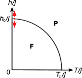
Figure 1: Left: One-dimensional spin-ring with $L=12$ Ising spins. Right: Phase diagram of the Gaussian RFIM (corresponding to Ref. Hartmann and Rieger, 2002), where “F” denotes the ferromagnetic and “P” the paramagnetic phase, both separated by the phase boundary.

The universality class of the model can be changed by varying $\sigma$. For $0<\sigma<1/3$ the critical exponents assume their mean-field (MF) values and for $1/3<\sigma<1/2$ the model is assumed to be in the non-MF region Monthus and Garel (2011). If $\sigma>1/2$, one expects no phase transition, Bray (1986); Weir et al. (1987); Aizenman and Wehr (1990a, 1989); Aizenman and Wehr (1990b); Cassandro et al. (2009); Monthus and Garel (2011) i.e. the critical random-field strength $h_{c}=0$ for $T=0$.

The MF values Bray (1986); Weir et al. (1987); Monthus and Garel (2011) of the critical exponents are $\alpha=0$, $\beta=1/2$, $\gamma=1$ and $\nu=1/\sigma$. In the non-MF domain, i.e. $1/3<\sigma<1/2$ the correlation length exponent $\nu$ is not known exactly, so only the relations Monthus and Garel (2011)

$$\frac{2-\alpha}{\nu}=1-\sigma\quad\quad\frac{\beta}{\nu}=\frac{1}{2}-\sigma\quad\quad\frac{\gamma}{\nu}=\sigma$$ (2)

are known analytically exact. But if, e.g., $\alpha$ is known ($\alpha=0$ seems plausible from the results presented below), the first relation in Eqs. (2) allows the determination of $\nu$ and thus of the other exponents.

Here, we focus on $\sigma=0.25$, which belongs to the MF region, $\sigma=0.4$ corresponding to the non-MF domain, $\sigma=1/2$ right at the predicted border between non-MF region and the domain without a phase transition and $\sigma=1$ from the $h_{c}=0$ region.

III Obtaining Ground States

The critical behavior of a Gaussian RFIM along the phase boundary is controlled by the zero-temperature fixed point Bray and Moore (1985). Therefore, it is convenient to study the RFIM at $T=0$ and to alter the random field strength $h$ to cross the phase boundary (see arrow in Fig. 1). For the calculation of the exact ground state at $T=0$ for a given realisation the undirected graph is mapped to a directed network Picard and Ratliff (1975). The maximum flow on this network is then calculated using a Push-and-Relabel algorithm Goldberg and Tarjan (1988), whereof an efficient implementation exists in the LEDA-library GmbH (2010). These algorithms have a polynomial running time Ahuja et al. (1993) and are faster than Monte-Carlo simulations (see e.g. Ref. Rieger, 1995), because no equilibration time is needed and the ground state is exact. After one has obtained the maximum flow, the directed network is mapped back to a ground-state spin configuration.

More details about the mapping to a directed network can be found in Ref. Hartmann and Rieger, 2002.

IV Observables

After obtaining the spin configuration of a ground state, we calculate physical quantities of interest. First, we fix $H=0$ and use $H>0$ only for the calculation of the susceptibility. The average magnetization per spin is given by

$$m=[|M|]_{h}=\left[\left|\frac{1}{N}\sum_{i}S_{i}\right|\right]_{h},$$ (3)

where $N\equiv L$ is the number of spins and $[\cdotp]_{h}$ denotes average over disorder. This averaging for fixed $h$ is performed over different realisations of graphs and random fields $\{B_{i}\}$, where for each configuration of long-range bonds one random-field realisation is used.

The Binder cumulant Binder (1981) is calculated via

$$g(L,h)=\frac{1}{2}\left(3-\frac{[M^{4}]_{h}}{[M^{2}]^{2}_{h}}\right),$$ (4)

where in comparison to the original quantity the thermal average is omitted, because $T=0$ and the ground state is nondegenerate for a Gaussian RFIM.

To determine a specific-heat-like quantity Hartmann and Young (2001) at $T=0$ we measure the bond energy

$$E_{J}=-\frac{1}{N}\sum_{i<j}\varepsilon_{ij}\;S_{i}\;S_{j}\,.$$

Now, we are able to differentiate $E_{J}$ numerically with respect to $h$ by calculating a finite central difference

$$C\left(\frac{h_{1}+h_{2}}{2}\right)=\frac{[E_{J}(h_{1})]_{h}-[E_{J}(h_{2})]_{h}}{h_{1}-h_{2}},$$ (5)

which results in the specific-heat-like quantity $C$. The values $h_{1}$ and $h_{2}$ are two consecutive values of the random-field strength $h$, which have to be chosen appropriately.

The disconnected susceptibility is given by

$$\chi_{\text{dis}}=L^{d}\;[M^{2}]_{h},$$ (6)

in which $d=1$ in our case.

For the determination of the susceptibility five different field strengths $H_{n}=n\cdot H_{L}$ with $n\in\{0,4\}$ of the homogeneous external field are applied to the system for each realisation and each value of $h$. A parabolic fit (for details see Ref. Ahrens and Hartmann, 2011) to the datapoints yields the zero-field susceptibility

$$\chi=\left.\frac{\text{d}m}{\text{d}H}\right|_{H=0},$$

which is given by the slope of the parabola at $H=0$.

IV.1 Scaling in the non-mean-field region

For $\sigma>1/3$, i.e. below the upper critical dimension the observables should scale close to the critical point $h_{c}$ like expected from finite-size scaling (FSS) theory (see e.g. Ref. Yeomans, 1992).

The magnetization should scale like

$$m(h)=L^{-\beta/\nu}\;\widetilde{m}([h-h_{c}]\;L^{1/\nu}),$$

with some scaling function $\widetilde{m}$.

Close to the critical point, being a dimension-less quantity, the Binder parameter is assumed to have the following scaling behavior:

$$g(L,h)=\widetilde{g}([h-h_{c}]\;L^{1/\nu}).$$

The scaling behavior of the singular part of the specific-heat-like quantity is

$$C(h)=L^{\alpha/\nu}\;\widetilde{C}([h-h_{c}]\;L^{1/\nu}),$$ (7)

and finite-size scaling predicts for the disconnected susceptibility

$$\chi_{\text{dis}}(h)=L^{\overline{\gamma}/\nu}\;\widetilde{\chi}_{\text{dis}}([h-h_{c}]\;L^{1/\nu}).$$ (8)

The scaling behavior for the susceptibility is expected to be

$$\chi(h)=L^{\gamma/\nu}\;\widetilde{\chi}([h-h_{c}]\;L^{1/\nu}).$$

IV.2 Scaling in the mean-field region

For $0<\sigma<1/3$, i.e. above the upper critical dimension $d_{u}$ the usual finite-size scaling forms (cf. section IV.1) are not valid (see e.g. Refs. Luijten and Blöte, 1997; Jones and Young, 2005; Ahrens and Hartmann, 2011; Monthus and Garel, 2011). At the critical point, the correlation length of the finite system is no longer proportional to the system size $L$, but behaves like Jones and Young (2005); Ahrens and Hartmann (2011) $L^{d/d_{u}}$ and $L$ needs to be replaced Jones and Young (2005) by $\ell=a_{1}L^{d/d_{u}}$ in the FSS relations, where $a_{1}$ is a nonuniversal constant. Therefore, the correlation length scaling exponent $\nu$ has to be replaced in the preceding section IV.1 to obtain scaling relations for the mean-field region by Botet et al. (1982); Ahrens and Hartmann (2011)

$$\nu^{*}=\frac{d_{u}}{d}\;\nu_{\text{MF}}=3,$$ (9)

where $d_{u}=3\sigma$, $d=1$ and $\nu_{\text{MF}}=1/\sigma$ has been used. We therefore use $1/\nu^{*}=1/3$ instead of $1/\nu_{\text{MF}}=\sigma$ in the mean-field case $\sigma=1/4$ for our finite-size scaling analyses.

IV.3 Corrections to scaling at the lower and upper critical dimension

Right at the upper critical dimension ($d_{u}=4$) of the $\phi^{4}$-model, Brézin Brézin (1982) showed that the correlation length $\xi\propto L(\log L)^{1/4}$. So, for $d=d_{u}$ logarithmic corrections Jones and Young (2005); Ahrens and Hartmann (2011) to scaling are expected and the lattice length $L$ has to be replaced by $\ell=a_{2}L(\ln L)^{1/d_{u}}$.

Right at the lower critical dimension Leuzzi and Parisi Leuzzi and Parisi (2013) recently proposed a logarithmic finite-size scaling. For the Binder parameter as well as for the two-point disconnected correlation function good data collapses for $\rho=1.5$ (corresponding to $\sigma=0.5$) and $(h/J)_{c}=2.31(5)$ were achieved with logarithmic scaling.

In section V.3 we investigate the scaling behavior of some observables for $\sigma=0.5$ to check whether an algebraic or logarithmic scaling appears.

V Results

Next, we present the simulation results for the different values of $\sigma\in\{0.25,0.4,0.5,1\}$. System sizes from $L=2^{6}=64$ up to $L=2^{19}=524288$ spins and $10^{3}$ to $10^{6}$ samples were used. All shown data points are averages over the given number of samples and the statistical errors result from the bootstrap resampling method Hartmann (2009). The average number of long-range bonds per node is fixed to $z=6$. For the determination of the susceptibility, the applied field stride $H_{L}$ of the homogeneous field is shown in Tab. 1.

Figure 2: Average magnetization as a function of random-field strength $h$ for different system sizes $L$ and $\sigma=1/4$. Data points are averaged over at least $10^{3}$ samples and error bars result from 30 bootstrap samples. Lines are guides to the eyes only.

V.1 Mean-field region $\sigma=0.25$

Figure 2 shows the average magnetization per spin calculated by formula (3) as a function of disorder strength $h$. For small $h$ the system is in the ferromagnetic ordered phase, where $m(h)\approx 1$ and for larger values of the random-field strength the system is in the paramagnetic phase, where $h\rightarrow 0$. With increasing $L$ the curves get steeper suggesting a phase transition at a critical value of $h_{c}\approx 5$.

Figure 3: Binder parameter as a function of random-field strength $h$ for different system sizes $L$ and $\sigma=1/4$. Data points are averaged over at least $10^{3}$ samples and error bars result from 30 bootstrap samples. Lines are guides to the eyes only.

To determine this critical random-field strength more accurate, we calculate the Binder parameter, given in equation (4). Finite-size scaling theory predicts an intersection of the curves for the Binder cumulant for different system sizes at the critical point $h_{c}$. This can be seen in Fig. 3, from which we estimate $h_{c}\approx 5.1$.

Figure 4: Specific-heat-like quantity $C$ averaged over at least $10^{4}$ samples as a function of random-field strength $h$ for different system sizes $L$ and $\sigma=1/4$. Dashed lines are example fits for three system sizes with fourth-order polynomials to obtain the maxima of $C$.

Next, we investigate the specific-heat-like quantity $C$, where we choose $h$ values with distance $h_{1}-h_{2}=0.1$ in equation (5). Figure 4 shows the peaks of $C$ close to the critical point for different system sizes. One can observe that with increasing system size $L$ the peak height grows as well as the peak position shifts to larger values of $h$.

Figure 5: Double logarithmic plot of the peak heights of the specific-heat-like quantity $C$ as a function of system size $L$ for $\sigma=1/4$. Dotted line denotes logarithmic fit (10) for $L>256$ with parameters $a=0.33(7)$, $b=0.15(1)$ and dash-dotted line is an algebraic fit (11) also for $L>256$ with parameters $c=2.49(7)$, $d=-1.52(9)$ and $k=-0.17(1)$. Inset: Peak positions of $C$ as a function of $L$. Dash-dotted line denotes a fit for $L>2048$ by Eqs. (13), where $h_{c}=5.13$, $a_{2}=-2.7$ and $1/\nu^{*}=0.215$. Dotted line denotes same fit but fixed $1/\nu^{*}=1/3$, resulting in $h_{c}=5.03$ and $a_{2}=-5.82$.

This impression is confirmed by Fig. 5. Apparently, both the peak heights and the peak positions behave like a power-law with added constant as a function of the number of spins $L$: In fact we tested three different possible behaviors of the peak heights of the specific-heat-like quantity:

$$C_{\text{max}}^{\text{log}}(L) =a+b\ln L,$$ (10)

$$C_{\text{max}}^{\text{alg}}(L) =c\cdot(1+d\cdot L^{k}),$$ (11)

$$C_{\text{max}}^{\text{corr alg}}(L) =c_{2}\;L^{\alpha/\nu^{*}}\cdot(1+d_{2}\cdot L^{k_{2}}),$$ (12)

a logarithmic divergence, an algebraic behavior and an algebraic function with a correction term.

All fits are least-squares fits with a reduced chisquare of $\chi_{\text{red}}^{2}=\sum_{i}^{n}[(y_{i}-f(x_{i}))/\Delta_{i}]^{2}/n_{\text{df}}$, where the degrees of freedom of the fit are $n_{\text{df}}=n-n_{\text{param}}$, which is the difference between the number of datapoints $n$ and the number of parameters $n_{\text{param}}$ in the fit-function $f$. The datapoints $(x_{i},y_{i}\pm\Delta_{i})$ have an error of $\Delta_{i}$.

The logarithmic fit yields a reduced chisquare of $\chi_{\text{red}}^{2}\approx 200$ for system sizes $L>256$ and $\chi_{\text{red}}^{2}\approx 118$ for $L>512$, which is quite bad. A better result is obtained with the algebraic fit where $\chi_{\text{red}}^{2}=6.9$ ($L>256$) or $\chi_{\text{red}}^{2}=4.2$ for $L>512$, which is o.k. Because of these fits, a logarithmic divergence of the specific-heat-like quantity can be excluded. The fit by equation (12) does not converge for values $\alpha/\nu^{*}>0$, so that we conclude $\alpha/\nu^{*}=0$.

Figure 6: Susceptibility $\chi$ averaged over at least $10^{4}$ samples with error bars resulting from 30 bootstrap samples as a function of random-field strength $h$ for different system sizes $L$ and $\sigma=1/4$. Dashed lines are example fits for three system sizes with a Gaussian and additional sigmoidal term to obtain the maxima of $\chi$. Note that for $L=64$ and $L=128$ $\chi$-values up to $h=8$ were used to determine the maxima, but are omitted here for clarity of the plot.

For the peak positions, fits of an algebraic function

$$h_{\text{max}}(L)=h_{c}+a_{2}\cdot L^{-1/\nu},$$ (13)

where $\nu=\nu^{*}$ should apply for the MF case $\sigma=1/4$.

	$\sigma=0.25$		$\sigma=0.4$		$\sigma=0.5$		$\sigma=1.0$
$L$	$H_{L}$	$N_{\text{samp}}$	$H_{L}$	$N_{\text{samp}}$	$H_{L}$	$N_{\text{samp}}$	$H_{L}$	$N_{\text{samp}}$
		$/10^{4}$		$/10^{4}$		$/10^{4}$		$/10^{4}$
64	0.300	100	–	–	–	–	–	–
128	0.065	10	–	–	–	–	–	–
256	0.050	$5$	0.016	$10$	0.0150	$5$	0.0250	$5$
512	0.039	$5$	0.011	$10$	0.0110	$5$	0.0180	$5$
1024	0.030	$5$	0.008	$5$	0.0075	$5$	0.0125	$5$
2048	0.023	$5$	0.006	$5$	0.0050	$5$	0.0090	$5$
4096	0.018	$5$	0.004	$5$	0.0038	$5$	0.0063	$5$
8192	0.014	$5$	0.003	$5$	0.0027	$5$	0.0044	$5$
16384	0.011	$5$	0.002	$1$	0.0019	$5$	0.0031	$1$

Table 1: System sizes $L$, smallest external fields $H_{L}$ and number of samples $N_{\text{samp}}$ which are used to determine the susceptibility for the given values of $\sigma$.

Due to the change of curvature of the data, see inset of Fig. 5, only system sizes $L>2048$ were used for the fit. The fit by formula (13) gives $\chi_{\text{red}}^{2}=9.6$, $h_{c}=5.13\pm 0.10$ and $1/\nu^{*}=0.215\pm 0.071$. This value for $1/\nu^{*}$ is a bit off but still compatible within two error bars with the expected $1/\nu^{*}=1/3$. We also test, see the inset of Fig. 5, a fit by equation (13) for $L>2048$ with fixed $1/\nu^{*}=1/3$. It yields $\chi_{\text{red}}^{2}=13.6$ and the curves of both fits are quite close to each other, so $1/\nu^{*}=1/3$ seems possible. Due to these results, i.e., strong finite-size corrections, the poor quality of the data for smaller system sizes and therefore the small amount of usable data points for the fits, the found value of $1/\nu^{*}$ is not included in the average given in Tab. 2.

Figure 6 shows the maxima of the zero-field susceptibility $\chi$, where the smallest external fields $H_{L}$, which were used to determine this quantity are given in Tab. 1.

Figure 7: Double logarithmic plot of the peak heights of the susceptibility $\chi$ as a function of system size $L$ for $\sigma=1/4$. Dashed-dotted line denotes algebraic fit (14) with parameters $a_{3}=0.075$ and $\gamma/\nu^{*}=0.33$ (fixed). Dotted line is an algebraic fit with a correction term (15) with parameters $a_{4}=0.170$, $\gamma/\nu^{*}=0.33$ (fixed), $d_{3}=-1.330$ and $k_{3}=-0.199$. Inset: Peak positions of $\chi$ as a function of $L$. Dotted line is a fit by Eq. (13) with parameters $h_{c}=4.993$, $a_{2}=2.39$, $1/\nu^{*}=0.33$ (fixed) and dash-dotted line denotes a fit by Eq. (16), where $h_{c2}=5.073$, $a_{5}=0.6$, $1/\nu^{*}=0.33$ (fixed), $d_{4}=33$, $k_{4}=-0.54$. Horizontal lines are $h_{c2}=5.073$ and $h_{c}=4.993$, respectively.

It seems that the larger the system size $L$, the larger the peak height of $\chi$ and the (slightly) more the peak position is at larger values of $h$. This behavior is shown in Fig. 7, where the maxima are expected to increase like

$$\chi_{\text{max}}(L)=a_{3}\cdot L^{\gamma/\nu^{*}}.$$ (14)

A fit to the data with fixed value $\gamma/\nu^{*}=0.33$ yields a reduced chisquare of $\chi_{\text{red}}^{2}\approx 2600$. As visible from the double logarithmic plots in Fig. 7, the data exhibits a clear curvature, incompatible with a pure power law. When taking finite-size corrections into account and using

$$\chi_{\text{max}}(L)=a_{4}\cdot L^{\gamma/\nu^{*}}\cdot(1+d_{3}\cdot L^{k_{3}})$$ (15)

again with fixed value $\gamma/\nu^{*}=0.33$, this results in $k_{3}=-0.199\pm 0.009$ and $\chi_{\text{red}}^{2}=0.31$. This reduced chisquare value is much smaller than for a fit without corrections. Thus, the value of $\gamma/\nu^{*}$ seems to be appropriate.

The fits to the peak positions of the susceptibility are shown in the inset of Fig. 7. A fit by formula (13) with fixed value $1/\nu^{*}=0.33$ fit parameter yields $h_{c}=4.993\pm 0.023$ with $\chi_{\text{red}}^{2}=33.6$.

Figure 8: Data collapse of the Binder parameter for $\sigma=1/4$. Collapse was performed for system sizes $L=4096$ up to $L=131072$.

A fit with correction term

$$h_{\text{max}}(L)=h_{c2}+a_{5}\cdot L^{-1/\nu}\cdot(1+d_{4}\cdot L^{k_{4}}),$$ (16)

where here $\nu=\nu^{*}$ and fixed $1/\nu^{*}=0.33$ gives $\chi_{\text{red}}^{2}=7.1$. This value is smaller than for a fit without corrections, so we keep the chosen value $1/\nu^{*}=0.33$. Further parameters of the fit by equation (16) are $h_{c2}=5.073\pm 0.057$ and $k_{4}=-0.54\pm 0.72$.

Figure 9: Data collapse of the magnetization for $\sigma=1/4$. Collapse was performed for system sizes from $L=4096$ up to $L=131072$. Smaller system size is shown for comparison.

Next, we perform data collapses of the observables to obtain estimates for the critical exponents with another independent approach. For the determination of the best collapse we used a python script Melchert (2009). Figure 8 shows the collapse for the Binder cumulant with parameters $h_{c}=5.117\pm 0.005$ and $1/\nu^{*}=0.357\pm 0.027$. The value of $1/\nu^{*}$ is compatible with the expected value $1/\nu^{*}=1/3$ within the error bar. The quality of the collapse is very high below the critical point. Above the critical point, only the two smallest system sizes exhibit a notable deviation from a joint scaling curve, which can be attributed to finite-size corrections to scaling.

Figure 10: Data collapse of the specific-heat-like quantity for $\sigma=1/4$. System sizes from $L=2048$ up to $L=131072$ were used for the collapse. Note that $\alpha=0$ is fixed.

The data collapse of the magnetization is presented in Fig. 9. The parameters of the collapse, which has a high quality around the phase transition $h-h_{c}\approx 0$, have the following values $h_{c}=5.185\pm 0.003$, $1/\nu^{*}=0.363\pm 0.020$ and $\beta/\nu^{*}=0.208\pm 0.003$. This means $\beta=0.573\pm 0.041$, which is compatible within two standard error bars with the mean-field value $\beta=1/2$.

The result of the data collapse for the specific-heat-like quantity is shown in Fig. 10, where the important parameters $h_{c}=5.168\pm 0.004$, $1/\nu^{*}=0.317\pm 0.010$ and $\alpha=0$ (fixed) were used. Below the critical point, the collapse is poor, whereas around and above the critical point it is quite good.

The data collapse of the susceptibility is shown in Fig. 11. The important parameters of the collapse are $h_{c}=5.108\pm 0.064$, $1/\nu^{*}=0.313\pm 0.064$ and $\gamma/\nu^{*}=0.387\pm 0.023$. The quality of the collapse is very good, except for smaller system sizes $L<2048$, where deviations especially around the critical point occur.

Finally, the data collapse of the disconnected susceptibility (not shown) for system sizes $L=2048$ up to $L=131072$ yields $h_{c}=5.146\pm 0.003$, $1/\nu^{*}=0.342\pm 0.001$ and $\bar{\gamma}/\nu^{*}=0.666\pm 0.005$. This results in $\bar{\gamma}=1.947\pm 0.020$ which is compatible with the mean-field value $\bar{\gamma}=2$ within three standard errors.

Figure 11: Data collapse of the susceptibility for $\sigma=1/4$. Collapse was performed for system sizes $L=2048$ up to $L=16384$. Smaller system sizes are included for comparison.

A summary of the results for all critical exponents is shown in Table 2. We have obtained these values by averaging the results obtained by different methods, respectively. The error bars are chosen such that they include the values obtained by the different methods. This should account for systematical errors, in particular corrections to scaling. This results in all values being compatible with the mean-field predictions.

		$h_{c}$	$1/\nu$	$\beta$	$\alpha$	$\gamma$	$\bar{\gamma}$
$\sigma=0.25$	m	5.13(6)	0.34(6)	0.62(13)	0	1.06(29)	1.98(39)
	t	3.9-6.6	0.33	0.5	0	1	2
$\sigma=0.4$	m	4.5(2)	0.30(6)	0.27(8)	0	1.50(54)	2.74(54)
	t	2.5	0.3	0.33	0	1.33	2.66
$\sigma=0.5$	m	3.7(2)	0.25(9)	0.06(3)	0	2.00(85)	3.8(13)
	t	–	0.25	0	0	2	4
$\sigma=1.0$	m	0	0.40(8)	0	0	2.19(53)	2.51(83)
	t	0	0.5	0	–	2	2

Table 2: Results of the ground-state calculations for the investigated values of $\sigma$ (line with “m”). For comparison the theoretical values Bray (1986); Weir et al. (1987); Grinstein and Mukamel (1983); Monthus and Garel (2011); Fisher et al. (2001); Aharony and Pytte (1983) are given, where for $\sigma\in\{0.4,0.5\}$ $\alpha=0$ was assumed to get estimates of the other exponents (cf. Eqs. (2)). Note that for $\sigma=0.25$ the value for $1/\nu^{*}$ is given here. The value $\gamma=2$ for $\sigma=1$ was obtained by calculating the susceptibility $\chi=\lim_{H\rightarrow 0}\partial m/\partial H\sim h^{-2}$ using the equilibrium magnetization from reference Fisher et al., 2001. Theoretical values for $\bar{\gamma}$ were obtained by using the Schwartz-Soffer equation (19), except for $\sigma=1$, where trivially $\bar{\gamma}/\nu=d=1$ from Eqs. (6) and (8).

V.2 Non-mean-field region $\sigma=0.4$

For the non-mean field region, we expect still a clear phase transition but with different exponents. We have performed simulations and analyses in the same way as for $\sigma=0.25$. For brevity, we omit most plots, since they look similar as for the mean-field case.

Figure 12: Binder parameter as a function of random-field strength $h$ for different system sizes $L$ and $\sigma=0.4$. Lines are guides to the eyes only. Inset: Data collapse of the Binder cumulant for $\sigma=0.4$ and system sizes $L=2048$ up to $L=32768$. Smaller sizes are shown for comparison.

As an example, Fig. 12 shows the Binder parameter as a function of the disorder strength $h$ for $\sigma=0.4$. One can see an intersection of all curves close to $h_{c}\approx 4.45$ indicating a phase transition at this point. The inset presents the data collapse of the Binder cumulant which seems quite good, as the curves for the different system sizes fall onto one curve. The parameters for this collapse were $h_{c}=4.454\pm 0.015$ and $1/\nu=0.300\pm 0.058$.

We have obtained critical exponents for the other quantities in the same way as discussed above. The results are summarized in Tab. 2. In particular, $1/\nu=0.30(6)$ agrees with $1/\nu=0.316(9)$ from reference Leuzzi and Parisi, 2013 (for $\rho=1.4$ in the cited paper).

V.3 Borderline case $\sigma=0.5$

The value of $\sigma=1/2$ was conjectured Bray (1986); Weir et al. (1987); Cassandro et al. (2009); Monthus and Garel (2011) to correspond to the lower critical dimension. Thus, so for $\sigma>1/2$ one has $h_{c}=0$. Nevertheless, right at the critical value $\sigma=\sigma_{c}=1/2$, the behavior could also correspond to $h_{c}>0$, as mathematical proofs Cassandro et al. (2009); Aizenman and Wehr (1990a, 1989); Aizenman and Wehr (1990b) do not exclude the possibility of a phase transition for $\sigma=\sigma_{c}$. We investigated this issue in the same way as for the cases $\sigma<1/2$.

The curves of the Binder cumulant (Fig. 13) for different system sizes do not show a clear intersection. This could be a hint towards $h_{c}=0$.

Figure 13: Binder cumulant as a function of the random field strength for $\sigma=1/2$. Inset: No clear intersection of the curves for different system sizes $L$ can be determined. Lines are guides to the eyes only.

Thus, we studied the peak positions of the specific-heat-like quantity as shown in Fig. 14. When fitting a power law Eq. (13) we obtained $h_{c}=3.899\pm 0.004$ and $1/\nu=0.307\pm 0.014$ with a quality of the fit of $\chi_{\text{red}}^{2}=1.5$. This strongly indicates $h_{c}\approx 3.9>0$. Note that we also fitted a power-law with correction term (16). The important parameters are $h_{c2}=3.898\pm 0.008$, $k_{4}=-1\pm 12$ and $1/\nu=0.302\pm 0.035$. The reduced chisquare is now $\chi_{\text{red}}^{2}=1.9$. To check for logarithmic scaling Leuzzi and Parisi (2013) another fit function was taken into account:

$$h_{\text{max}}(L)=h_{c3}+\frac{a_{6}}{\ln L},$$ (17)

which leads to $\chi_{\text{red}}^{2}=8.4$ with the parameters $h_{c3}=3.71\pm 0.01$ and $a_{6}=2.95\pm 0.12$. Thus, a logarithmic scaling assumption seems less compatible with our results than a power-law behavior (with corrections).

Furthermore, we obtained the susceptibility and the corresponding positions (and heights) of the peaks. In the inset of Fig. 14 the data for the peak positions of the susceptibility and fits are presented. The first one by equation (13) yields a reduced chisquare of $\chi_{\text{red}}^{2}=0.03$ with $h_{c}=3.869\pm 0.033$ and an exponent $1/\nu=0.316\pm 0.021$. The second fit by Eq. (17) yields with $h_{c3}=3.162\pm 0.023$ and $a_{6}=9.46\pm 0.19$ to $\chi_{\text{red}}^{2}=0.06$, so both fits are compatible with our data. And indeed, as the inset of Fig. 14 shows both curves agree very well in the range of the data points.

Thus, our results clearly support $h_{c}>0$ for $\sigma=0.5$. Although we cannot determine whether the finite-size scaling is of logarithmic or of power-law type, both suggest that $h_{c}>0$. Recent results which support our findings were provided by Ref. Garel, , where the Dyson hierarchical random-field model (cf. Ref. Monthus and Garel, 2011) for $\sigma=1/2$ was investigated numerically for system sizes up to $L=2^{21}$. These results strongly indicate that the magnetization converges for system sizes $L\rightarrow\infty$ to one common curve at $h_{c}>0$. In reference Leuzzi and Parisi, 2013, Binder cumulants of a one-dimensional RFIM on a Lévy lattice are studied. Finite-size scaling analysis of the Binder parameter at the value $\sigma=1/2$ (corresponding to $\rho=3/2$ in the cited paper) yielded Leuzzi and Parisi (2013) $(h/J)_{c}\approx 2.31(5)>0$.

Figure 14: Peak positions of the specific-heat-like quantity as a function of system size for $\sigma=1/2$. Dotted line is a fit by Eq. (13) with parameters $h_{c}=3.899$, $a_{2}=2.20$ and $1/\nu=0.307$. Dashed-dotted line is a fit by Eq. (16) with $h_{c2}=3.898$, $a_{5}=2.13$, $1/\nu=0.302$, $d_{4}=11$ and $k_{4}=-1$. Horizontal line denotes $h_{c}=3.899$. Solid line is a logarithmic fit by Eq. (17) with $h_{c3}=3.71$ and $a_{6}=2.95$. Inset: Peak positions of the susceptibility as a function of system size $L$. Dotted line is a fit by Eq. (13), where $h_{c}=3.869$, $a_{2}=5.84$ and $1/\nu=0.316$. Horizontal line denotes $h_{c}=3.869$. Solid line is a logarithmic fit by Eq. (17) with $h_{c3}=3.162$ and $a_{6}=9.46$.

Finally note that also the data points of the magnetization (not shown) for various system sizes converge for $L\rightarrow\infty$ to one single curve with $h_{c}\approx 4.0>0$. The complete set of resulting estimates for the critical exponents is again shown in Tab. 2.

V.4 Region without non-trivial phase transition $\sigma=1.0$

Finally we turn to the case $\sigma=1$ where we expect no phase transition. Fig. 15 shows the Binder parameter for various system sizes. One can see that there is no intersection between the curves for different system sizes, which means that $h_{c}=0$. This is supported by the fact that the curves of the magnetization (not shown) for different system sizes do not converge towards one curve for $L\rightarrow\infty$, in contrast to, e.g., the case $\sigma=1/4$ (cf. Fig. 2). Thus, the magnetization jumps from zero for any value $h>0$ to $m=1$ for $h=0$, meaning $\beta=0$. Nevertheless, for the specific heat-like quantity and the susceptibilities, we could study (not shown here) the behavior when approaching $h=0$ in the same way as for the previously discussed values of $\sigma$. This results in $\nu=0.40(8)$, $\alpha\approx 0$, $\gamma=2.19(53)$ and $\bar{\gamma}=2.51(83)$, as shown in Tab. 2.

Figure 15: Binder cumulant for $\sigma=1.0$ averaged over at least $10^{3}$ realisations. Lines are guides to the eyes only.

VI Conclusion and Outlook

We have studied exact ground states of one-dimensional ($d=1$) long-range random-field Ising magnets. The probability $p$ of placing a bond between two spins depends on the geometric distance $r$ of these spins as $p(r)\sim r^{-d-\sigma}$. Since polynomial-time running algorithms exist, based on a mapping to the maximum-flow problem, we could study large systems numerically with a high number of random samples. We studied the model for different values of $\sigma$, which are representatives for the different expected behavior of the model.

Table 2 summarizes the obtained values of the critical point and the critical exponents in comparison with the expected values from theory. In the mean-field case for $\sigma=0.25$ the critical exponents agree well within error bars with the theoretical values. The critical point is consistent with values found for the Dyson hierarchical version Monthus and Garel (2011) of the RFIM. In the non-mean-field region for $\sigma=0.4$, the exponents also agree well with theory. The critical point $h_{c}$ does not agree with the one found in reference Monthus and Garel, 2011, but these points are anyway non-universal.

In the borderline case $\sigma=0.5$, in particular the critical point $h_{c}>0$ is an interesting result, as only statements Bray (1986); Weir et al. (1987); Cassandro et al. (2009); Aizenman and Wehr (1990a, 1989); Aizenman and Wehr (1990b); Monthus and Garel (2011) of the existence of a finite-disorder phase transition for $\sigma\neq 1/2$ have been published so far. In addition, mathematical proofs Aizenman and Wehr (1990a, 1989); Aizenman and Wehr (1990b); Cassandro et al. (2009) do not exclude the possibility of $h_{c}>0$ for $\sigma_{c}=1/2$ at zero temperature. Recent work Leuzzi and Parisi (2013), which was performed independently and in parallel to our work, support $h_{c}>0$. In the cited work, an Imry-Ma argument (cf. also Refs. Bray, 1986; Weir et al., 1987; Cassandro et al., 2009; Monthus and Garel, 2011) is given and also calculations of exact ground states were carried out independently of our work, but it was restricted to the analysis of the Binder cumulant and few other observables. Nevertheless, all measured exponents agree with theory, if one assumes the theory (cf. Eqs. (2)) for $1/3\leq\sigma<1/2$ to be valid also at $\sigma=1/2$. Note that the value of $\beta$ is off by a few error bars, but for values close to zero, one would have to go to large system sizes to see the limiting behavior.

For $\sigma=1$, the measured critical point $h_{c}=0$ agrees with theory as well as the value for $\beta$. Nevertheless, the expected jumps Aharony and Pytte (1983) in the magnetization as $\beta=0$ were not observed. As usual for first-order transitions, a real jump can be expected to be visible only in the thermodynamic limit, i.e. for huge system sizes.

The found value of the correlation length exponent $\nu$ does agree with theory within two error bars, where $\nu=1/2$ is predicted Aharony and Pytte (1983); Bray and Moore (1985) for $\sigma=1$. Both values for $\gamma$ and $\bar{\gamma}$ are compatible with the expected values if the error bars are taken into account.

Next, we check the Rushbrooke equality Essam and Fisher (1963) for the different values of $\sigma$:

$$\alpha+2\beta+\gamma=2.$$ (18)

For $\sigma=0.25$ one gets the value $\alpha+2\beta+\gamma=2.30(54)$, which fulfills equation (18) within the standard error bar. For $\sigma=0.4$, formula (18) yields $\alpha+2\beta+\gamma=2.04(70)$, which is in good agreement with the expected value when the statistical error is taken into account. For the borderline case $\sigma=0.5$ between non-mean-field region and the region without a non-trivial phase transition, one obtains $\alpha+2\beta+\gamma=2.11(90)$, which fulfills equation (18) within error bars. In the region, where $h_{c}=0$ and thus $\sigma=1$, one gets $\alpha+2\beta+\gamma=2.19(53)$, which satisfies the scaling relation (18) within the statistical error. Because of the large error bars, resulting mainly from the large errors of $\gamma$, the tests of the Rushbrooke equality are not very significant.

We compare the theoretical and estimated values of the so-called droplet exponent $\theta$. In the mean-field case one gets Monthus and Garel (2011) $\theta_{\text{MF}}=\gamma_{\text{MF}}/\nu_{\text{MF}}=1/\nu_{\text{MF}}=\sigma$. For $\sigma=0.25$, we cannot check this directly, as we have measured $1/\nu^{*}$ rather than $1/\nu$. But according to Eq. (9) we get $1/\nu=0.253\pm 0.048$ which agrees well with $\theta_{\text{MF}}=\sigma$. In the non-mean-field region one obtains $\theta=\bar{\gamma}/\nu-\gamma/\nu$. For $\sigma=0.4$ this yields $\theta=0.378(81)$, and for $\sigma=0.5$ we get $\theta=0.452(45)$. In the case $\sigma=0.4$ it agrees within one and for $\sigma=0.5$ within two error bars with the prediction $\theta=\sigma$ by Grinstein Grinstein (1976). But smaller deviations from this conjecture could not be determined as the error bars of these quantities are too large. In the case $\sigma=1$, we obtain $\theta=0.13(16)$ which is compatible with $\theta=0$ within the error bar.

The conjecture Grinstein (1976) $\theta=\sigma$ only holds for the Dyson hierarchical model Rodgers and Bray (1988). It was shown later, that this prediction was pertubatively wrong at higher orders Bray (1986) for models with interaction strengths which decay like a power-law in the distance. However, for our model, we cannot make a statement whether the conjecture $\theta=\sigma$ holds or not, because for $\sigma=0.4,0.5$ our data does not allow the determination of small deviations from this conjecture because of too large error bars.

In a two exponent scenario, the Schwartz-Soffer equation Schwartz and Soffer (1985)

$$\bar{\gamma}=2\gamma$$ (19)

would hold. For $\sigma=0.25$ formula (19) is valid, when the statistical error is taken into account. In the cases $\sigma=0.4$ and $\sigma=0.5$, equation (19) is also fulfilled within statistical errors. For $\sigma=1$ the Schwartz-Soffer equation does not hold.

To summarize, the critical exponents for the investigated values $\sigma\in\{0.25,0.4,0.5,1\}$ agree well with theory, most values within one, few within two error bars. This deviation might be due to too large system sizes which are needed to see the infinite-size behavior. The Rushbrooke equality is fulfilled for all studied values of $\sigma$. The droplet exponent $\theta$ agrees well with theory for $\sigma\in\{0.4,0.5,1\}$, although a statement if the conjecture $\theta=\sigma$ holds is not possible. The two-exponent scenario is supported by the confirmation of the Schwartz-Soffer equation for $\sigma\in\{0.25,0.4,0.5\}$.

For the critical case $\sigma=1/2$, it was found that $h_{c}>0$, as for other recent numerical studies on the Dyson hierarchical model Monthus and Garel (2011) and for the same diluted model Leuzzi and Parisi (2013) as studied here. This is an interesting result, because with the Imry-Ma argument Bray (1986); Weir et al. (1987); Cassandro et al. (2009); Monthus and Garel (2011) only conclusions for the cases $\sigma<1/2$ or $\sigma>1/2$ are possible. Rigorous studies Aizenman and Wehr (1990a, 1989); Aizenman and Wehr (1990b); Cassandro et al. (2009) do also not exclude $\sigma=1/2$ as possible value of a finite-disorder phase transition at zero temperature. Our data allows no conclusion about the type of finite-size scaling behavior, as both an algebraic as well as a logarithmic behavior is possible.

For future studies, it could be of interest to study the same diluted long-range model on higher dimensional lattices. At least $d=2$ and $d=3$ should be accessible using the highly efficient maximum-flow algorithms used here.