Abstract

We propose an efficient optical electromagnetically induced transparency (EIT) cooling scheme for a cantilever with a nitrogen-vacancy center attached in a non-uniform magnetic field using dynamical Zeeman effect. In our scheme, the Zeeman effect combined with the quantum interference effect enhances the desired cooling transition and suppresses the undesired heating transitions. As a result, the cantilever can be cooled down to nearly the vibrational ground state under realistic experimental conditions within a short time. This efficient optical EIT cooling scheme can be reduced to the typical EIT cooling scheme under special conditions.

OCIS codes: (140.3320) Laser cooling; (260.7490) Zeeman effect; (270.1670) Coherent optical effects; (120.4880) Optomechanics

1 Introduction

Micro- and nano-mechanical resonators (MRs) [1, 2] exhibit both classical and quantum properties [3], which are relevant in fundamental physics and have various applications, such as entanglement between mesoscopic objects [4, 5], ultra-sensitive measurements [3, 6, 7], quantum information processing [8], and biological sensing [9].

Different from the classical properties of the MRs at room temperature, the quantum properties of the MRs are presented only at sufficiently low temperatures where the thermal fluctuations are suppressed. To suppress the thermal fluctuations of the MRs and study their quantum properties, various ground-state cooling schemes have been proposed, such as sideband cooling [10, 11, 12, 13, 14, 15, 16], cooling with static electrical interaction without any auxiliary qubit or photonic systems [17], hot thermal light cooling [18], time-dependent control cooling [17, 19], cooling method based on quadratic coupling [20], measurement-based cooling [21], and dynamic dissipative cooling [22]. Experimentally, efficient cooling of a MR with high frequency $\omega_{m}\simeq 2\pi\times 6$ GHz down to the ground state (with an average phonon number $\langle n\rangle\simeq 0.07$) was achieved with a direct refrigerator of 25 mK [23]. For most relevant MRs with lower frequencies, only a few efficient cooling experiments have been achieved with the final $\langle n\rangle<1$ [11, 24] via the sideband cooling scheme.

By contrast, in the cooling of vibrational motion of trapped ions instead of MRs, there are some more efficient optical cooling schemes besides the sideband cooling to achieve the ground-state cooling with the final average phonon number much less than $\mathrm{1}$, such as the electromagnetically induced transparency (EIT) cooling of vibrational motion of trapped ions [25, 26] through the suppression of undesired transitions [25, 26, 27], and the Stark shift cooling based on the Stark shift gate [27]. Those schemes remind us of using the similar cooling schemes to cool the motion of massive MRs.

However, neither the EIT cooling [25, 26] nor the Stark shift cooling [27] schemes in trapped ion systems can be directly applied to the MR, since the direct optical Lamb-Dicke parameter for the MR is too small to couple the vibrational motion of the MR with a qubit for the small amplitude of the zero point fluctuation. Recently, a microwave-based EIT cooling scheme [28] was proposed in a MR electromechanical system, in which large effective Lamb-Dick parameter can be achieved by controlling the applied magnetic field on a flux qubit. An attractive alternative is to replace the flux qubit with a nitrogen-vacancy (NV) center, which has important advantages including operating temperatures from 4 to 300 K, stable fluorescence even in small nanodiamonds, long spin lifetimes, optical initialization and readout, biological compatibility, as well as available quantum memory that can be encoded in proximal nuclear spins [29]. The first MR cooling scheme based on the NV center was proposed by Rabl et al. in Ref. [30], where it was shown that the magnetic-tip-attached MR could be strongly coupled to the NV center through a strong magnetic field gradient (MFG). The Lamb-Dicke parameter increases with increasing MFG, making it possible to cool the MR with a small frequency. This scheme is capable of producing an arbitrary quantum superposition of the cantilever states [30] and the essential ingredient of this scheme, the strong MFG coupling, has already been demonstrated in the experiment [31]. Nevertheless, this cooling scheme is based on microwave and is efficient in the resolved sideband regime. It is desirable to develop an optical cooling scheme that remains efficient in the non-resolved sideband regime, is faster and more efficient.

To this end, we present in this work an optical EIT cooling scheme for a cantilever with a NV center attached, which can rapidly cool the cantilever resonator down to nearly the vibrational ground state in the non-resolved sideband regime. Our scheme consists of two essential ingredients which are similar to Ref. [30]. The first ingredient is the negatively charged NV center attached at the end of a cantilever. The NV center serves as a $\mathrm{\Lambda}$-type three-level system, exhibiting quantum interference when two applied lasers are tuned to the two-photon resonance. The second ingredient is the strong MFG, which can couple the internal states of the NV center to the vibrational motion of the cantilever. Then, with the external light fields applied, off-resonant and undesired carrier transitions are suppressed, while the desired cooling transitions are enhanced like in the typical EIT coolings [25, 26]. As a result, our scheme can cool the vibrational motion of the cantilever close to its ground state. The main components needed in our scheme are experimentally available by using the current laboratory technology, e.g., the manipulation of a NV center with optical lights [34, 35] and the coupling of a NV center with the nanowire [31].

Our cooling scheme differs significantly from the previous ones [30, 32, 27, 33]. First, our scheme uses optical lights to achieve an effective EIT cooling. The carrier transition that dominates the heating process [28] is completely suppressed by the quantum interference effect, so it is efficient in the non-resolved sideband regime, with the maximal cooling rate close to the MFG coupling strength. By contrast, the previous NV center based scheme [30] uses microwaves and is efficient in the resolved sideband regime, with the maximal cooling rate much smaller than the MFG coupling strength. Second, our effective EIT cooling scheme uses the MFG mechanical coupling of the resonator to the ground states of the NV center. By contrast, the mechanical coupling in the typical atomic EIT cooling scheme [32] involves both the ground state and the excited state of the atomic internal states. Third, compared with the Stark shift cooling [27, 33], our scheme has a simpler configuration, i.e., it does not require the light/microwave driven transition between the two ground states.

The rest of the paper is organized as follows. In Sec. 2, we describe the model, discuss the cooling process, and connect our Hamiltonian to the typical EIT Hamiltonian by a canonical transformation. In Sec. 3, we derive the analytical formula for the cooling and heating rates and calculate the final average phonon number. In Sec. 4, we check the robustness and efficiency of our scheme by comparing it to a fully numerical simulation. Finally, a brief conclusion is given.

2 Model and Cooling process

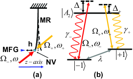
Fig. 1: (a) Schematic illustration of the optical scheme of NV center-assisted scheme of the effective optical EIT cooling. (b) Three internal energy levels of the NV center are coupled by two lasers satisfying the two-photon resonance $\Delta_{+}=\Delta_{-}$. The cantilever vibration is coupled to the NV center by a strong MFG. $\gamma_{+}$ ($\gamma_{-}$) is the decay from the excited state $|A_{2}\rangle$ to the ground state $|-1\rangle$ ($|+1\rangle$), which includes the electron leaking from and pumped into the nearly closed three-level for $|A_{2}\rangle$ and $|\pm 1\rangle$ (see Appendix A for details).

The system under consideration is a negatively charged NV center attached at the end of a nano-mechanical cantilever in a spatially non-uniform magnetic field. The NV center consists of a substitutional nitrogen atom and a neighboring carbon vacancy. The electronic ground state of the NV center is an $S=1$ spin triplet with a zero field splitting of $\mathrm{2\pi\times 2.87}$ $\mathrm{GHz}$ between the $m_{s}=0$ sublevel $\left|0\right\rangle$ and the $m_{s}=\pm 1$ sublevels $\left|\pm 1\right\rangle$ due to spin-spin interactions, where $m_{s}$ is the projection of the total electron spin $S=1$ along the $z$ (N-V) axis. According to the group theoretical analysis [36, 37], we assume that a $\sigma^{-}$- ($\sigma^{+}$-) polarized laser with the Rabi frequency $\Omega_{-}$ ($\Omega_{+}$) and light frequency $\omega_{-}$ ($\omega_{+}$ ) is applied to selectively couple the ground state $\left|+1\right\rangle$ ($\left|-1\right\rangle$) to the excited state $\left|A_{2}\right\rangle$ [36, 37, 38] as sketched in Fig. 1. Thus the three states $\left|\pm 1\right\rangle$ and $\left|A_{2}\right\rangle$ form a $\Lambda$-type three-level system, which exhibits quantum interference when the frequencies of the two lasers are tuned to two-photon resonance. In addition to decaying to the ground states $|\pm 1\rangle$ by spontaneous emission, the excited state $|A_{2}\rangle$ also has a small probability to decay non-radiatively to the metastable state $|^{1}A_{1}\rangle$ and then to the ground state $|0\rangle$. To prevent the leakage out of the $\Lambda$ system, we apply a recycling laser to excite $|0\rangle$ to another excited state $|E_{y}\rangle$, which then decays back into the states $|\pm 1\rangle$. In Appendix A, we show that the effect of these recycling transitions amounts to a small renormalization of the decay rate of $\left|A_{2}\right\rangle\rightarrow\left|+1\right\rangle$ ($\left|A_{2}\right\rangle\rightarrow\left|-1\right\rangle$) from $\gamma_{+1}$ ($\gamma_{-1}$) to $\gamma_{+}$ $(\gamma_{-}$).

In the presence of a non-uniform magnetic field $B(\mathbf{r})$ along the N-V symmetry axis of the NV center (defined as the $z$ axis), the Zeeman effect $g_{e}\mu_{B}B(\mathbf{\hat{r}})(\left|+1\right\rangle\left\langle+1\right|-\left|-1\right\rangle\left\langle-1\right|)$ couples the NV center to the vibration of the NV center or equivalently the vibration of the cantilever. Here, $\mathbf{\hat{r}}\equiv(\hat{x},\hat{y},\hat{z})$ is the position operator of the NV center attached to the tip of the cantilever and $B(\mathbf{\hat{r}})$ is the magnetic field on the NV center. As suggested in Refs. [33, 39], the Stark shift can be caused by the Zeeman effect, while there is no direct transition between the two ground states driven by an external light field in our work. For this reason, our scheme differs from the Stark shift cooling, but instead is an effective EIT cooling, i.e., it is connected to the typical EIT cooling Hamiltonians [25, 26] by a canonical transformation (to be shown below). Note that the excited state $\left|A_{2}\right\rangle$ is an equal mixture of $m_{s}=+1$ and $m_{s}=-1$ components, so its Zeeman effect is dominated by a second-order process mediated by another excited state $\left|A_{1}\right\rangle$. The large gap $\Delta_{A_{1}-A_{2}}\simeq$ $\mathrm{2\pi\times}$2.5 GHz between $\left|A_{2}\right\rangle$ and $\left|A_{1}\right\rangle$ makes this second-order contribution negligible for a weak magnetic field $\left|B(\mathbf{\hat{r}})\right|\ll\hbar\Delta_{A_{1}-A_{2}}/(g_{e}\mu_{B})\sim 10^{3}\ \mathrm{G}$. Taking the direction of the cantilever vibration as the $x$ axis and the equilibrium position of the cantilever tip (or equivalently the NV center) as the origin $\mathbf{r}=0$, the magnetic field $B(\mathbf{\hat{r}})=B(\hat{x},0,0)\equiv B(\hat{x})$ can be expanded as $B(\hat{x})\approx B(0)+B^{\prime}(0)\hat{x}$. The zeroth-order term $g_{e}\mu_{B}B(0)(\left|+1\right\rangle\left\langle+1\right|-\left|-1\right\rangle\left\langle-1\right|)$ is a constant Zeeman splitting that lifts the degeneracy of $\left|\pm 1\right\rangle$. The first-order term $g_{e}\mu_{B}B^{\prime}(0)(\left|+1\right\rangle\left\langle+1\right|-\left|-1\right\rangle\left\langle-1\right|)\hat{x}$ induces the coupling between the internal states of the NV center and the vibrational motion of the cantilever through the strong MFG [30, 31], where $\hat{x}=x_{0}(b+b^{\dagger})$ with $x_{0}=\sqrt{\hbar/(2M\omega_{m})}$ the amplitude of the zero-point fluctuation of the cantilever with mass $M$ and frequency $\omega_{m}$, and $b$ and $b^{\dagger}$ the corresponding annihilation and creation operators, respectively.

Without loss of generality, we take the Rabi frequencies $\Omega_{\pm}=\Omega_{0}$ as real numbers. Then, the total Hamiltonian for the coupled system reads ($\hbar=1$)

$$\begin{array}[]{ccl}H&=&\omega_{m}b^{\dagger}b+\omega_{A}\left|A_{2}\right\rangle\left\langle A_{2}\right|+g_{e}\mu_{B}B(0)(\left|+1\right\rangle\left\langle+1\right|-\left|-1\right\rangle\left\langle-1\right|)\\ &+&\frac{1}{2}\Omega_{0}(\left|A_{2}\right\rangle\left\langle+1\right|e^{-i\omega_{+}t}+\left|A_{2}\right\rangle\left\langle-1\right|e^{-i\omega_{-}t}+h.c.)\\ &+&\lambda(\left|+1\right\rangle\left\langle+1\right|-\left|-1\right\rangle\left\langle-1\right|)(b^{\dagger}+b).\end{array}$$ (1)

The first line describes the free evolution of the cantilever and the NV center with $\omega_{A}$ being the energy of state $|A_{2}\rangle$. The second line describes the selective excitation of the internal states of the NV center by two laser fields. The last line describes the MFG induced coupling between the internal states of the NV center and the vibration of the cantilever. The coupling strength $\lambda=$ $g_{e}\mu_{B}B^{\prime}(0)x_{0}$ is equal to the change of the Zeeman splitting over a zero-point fluctuation $x_{0}$. The physical picture for this interaction is that the first-order term $g_{e}\mu_{B}B^{\prime}(0)\hat{x}$, depending on the position of the NV center $\hat{x}$, induces an additional Zeeman splitting between the ground states $\left|+1\right\rangle$ and $\left|-1\right\rangle$. For a silicon cantilever with $(\mathrm{length,width,thickness})\simeq(25,0.1,0.1)\ \mathrm{\mu m}$, the cantilever vibrational frequency $\omega_{m}=2\pi\times 1$ MHz, the mass $M=1.22\times 10^{-14}$ kg, and the zero-point amplitude $x_{0}\simeq 1.6\times 10^{-13}\ \mathrm{m}$. Thus the coupling strength can reach $\lambda\simeq 2\pi\times 0.115\ \mathrm{MHz}$ [30, 40] for an achievable MFG value $B^{\prime}(0)\sim 2.4\times 10^{7}\ \mathrm{T/m}$. Consequently, the magnetic Lamb-Dicke parameter $\eta\equiv\lambda/\omega_{m}=g_{e}\mu_{B}B^{\prime}(0)x_{0}/\omega_{m}$ can be as large as $\eta\sim 0.115$ by using a strong MFG even for a massive MR with a small zero-point fluctuation $x_{0}$. This is in sharp contrast to the optical Lamb-Dicke parameter $\eta_{\mathrm{ion}}=2\pi x_{0}/\lambda_{\mathrm{light}}$ for the trapped ion, which scales as $x_{0}$ over the optical wavelength $\lambda_{\mathrm{light}}$. The MFG coupling of the NV center and its instantaneous influence on the NV center has been observed experimentally [31].

In the rotating frame defined by $|\psi^{\mathrm{rot}}(t)\rangle=e^{-iRt}|\psi(t)\rangle$ and $H^{\mathrm{rot}}=e^{-iRt}H(t)e^{iRt}+R$ with $R\equiv\omega_{+}\left|+1\right\rangle\left\langle+1\right|+\omega_{-}\left|-1\right\rangle\left\langle-1\right|$ [41], the Hamiltonian is time-independent:

$$\begin{array}[]{ccl}H^{\mathrm{rot}}&=&\omega_{m}b^{\dagger}b-\Delta\left|A_{2}\right\rangle\left\langle A_{2}\right|+\frac{1}{2}\Omega_{0}(\left|A_{2}\right\rangle\left\langle+1\right|+\left|A_{2}\right\rangle\left\langle-1\right|+h.c.)\\ &+&\lambda(\left|+1\right\rangle\left\langle+1\right|-\left|-1\right\rangle\left\langle-1\right|)(b^{\dagger}+b),\end{array}$$ (2)

where the detunings $\Delta_{\pm}\equiv\omega_{\pm}-[\omega_{A}\mp g_{e}\mu_{B}B(0)]$ of the $\sigma^{\pm}$ lasers have been chosen to satisfy the two-photon resonance condition $\Delta_{+}=\Delta_{-}\equiv\Delta$.

Then we make a canonical transformation $H^{\mathrm{rot}}\rightarrow H_{\mathrm{e}}\equiv e^{-iS}H^{\mathrm{rot}}e^{iS}$ with $S=-i\eta(\left|+1\right\rangle\left\langle+1\right|-|-1\rangle\left\langle-1\right|)\left(b-b^{\dagger}\right)$. Up to the first-order of the small Lamb-Dicke parameter $\left|\eta\right|\ll 1$, the Hamiltonian $H_{\mathrm{e}}$ takes the similar form as the one in the typical EIT cooling scheme [25, 26] as $H_{\mathrm{e}}(t)=H_{\mathrm{0}}+V$, in which

$$H_{\mathrm{0}}\equiv\omega_{m}b^{\dagger}b-\Delta\left|A_{2}\right\rangle\left\langle A_{2}\right|+\frac{\sqrt{2}}{2}\Omega_{0}(\left|A_{2}\right\rangle\left\langle b\right|+h.c.),$$ (3)

describes the motion of the NV center driven by the two lasers and

$$V=\eta\left(b-b^{\dagger}\right)(\frac{\Omega_{0}}{\sqrt{2}}\left|A_{2}\right\rangle\left\langle d\right|-h.c.),$$ (4)

is the coupling between the NV center and the cantilever. It is well known that the Hamiltonian of the NV center (in the absence of the MR) can be diagonalized as $H_{\mathrm{NV}}=E_{+}\left|+\right\rangle\left\langle+\right|+E_{-}\left|-\right\rangle\left\langle-\right|$ by the dark state $\left|d\right\rangle$ (with zero eigenenergy) and the two dressed states $\left|+\right\rangle=\cos\phi\left|A_{2}\right\rangle+\sin\phi\left|b\right\rangle$ and $\left|-\right\rangle=\sin\phi\left|A_{2}\right\rangle-\cos\phi\left|b\right\rangle$, where $\phi=(1/2)\cos^{-1}(-\Delta/\sqrt{2\Omega_{0}^{2}+\Delta^{2}})$ and the eigenenergies $E_{\pm}\equiv(-\Delta\pm\sqrt{2\Omega_{0}^{2}+\Delta^{2}})/2$ [42]. The linewidths of the two dressed states $\left|+\right\rangle$ and $\left|-\right\rangle$ are $\Gamma\cos^{2}\phi$ and $\Gamma\sin^{2}\phi$, respectively, which means that all the decay result from the decay $\Gamma=\gamma_{+}+\gamma_{-}$ from the excited state $\left|A_{2}\right\rangle$. In this situation, the state with the lowest energy is $\left|-\right\rangle$, whose dominant component is $\left|b\right\rangle$ (for $\Delta<0$) or $\left|A_{2}\right\rangle$ (for $\Delta>0$).

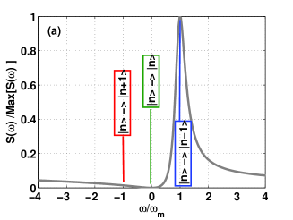
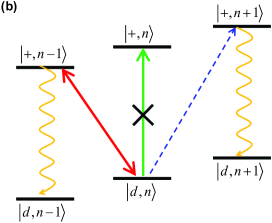
Fig. 2: (a) Absorption spectrum versus the frequency in our scheme. It is demonstrated that there is a dark dip for two-photon resonance in the absorption rate, and the quantum interference can be used to suppress the heating transitions $|n\rangle\rightarrow|n\rangle$ and $|n\rangle\rightarrow|n+1\rangle$ and enhance the cooling transition $|n\rangle\rightarrow|n-1\rangle$. The parameters are taken as $\omega_{m}=2\pi\times 1$ MHz, $\Gamma=15\omega_{m}$ , $\Omega_{0}=8\omega_{m}$, and $\Delta=31\omega_{m}$; (b) The cooling cycle of our scheme. The action of the external light fields (with the Rabi frequencies $\Omega_{0}$) and the Zeeman effect (with the coupling $\lambda$) can only create the red sideband transition $\left|d,n\right\rangle\rightarrow\left|+,n-1\right\rangle$ since the carrier transition between $\left|d,n\right\rangle$ and $\left|+,n\right\rangle$ and a blue sideband transition $\left|d,n\right\rangle$ and $\left|+,n+1\right\rangle$ are suppressed when two applied lasers are tuned to two-photon resonance. Then, if the decay is from $\left|+,n-1\right\rangle$ to $\left|d,n-1\right\rangle$, one phonon has been lost compared with the initial state, whereas if the transition is $\left|+,n-1\right\rangle\rightarrow\left|d,n\right\rangle$, the cycle will be repeated.

As sketched in Fig. 2, the cooling process in our scheme can be understood as a typical EIT cooling [25, 26]. From the initial state $\left|d,n\right\rangle$, the action of the external light fields (with the Rabi frequencies $\Omega_{0}$) and the Zeeman effect (with the coupling $\lambda$) can only create the red sideband transition $\left|d,n\right\rangle\rightarrow\left|+,n-1\right\rangle$ since both the carrier transition between $\left|d,n\right\rangle$ and $\left|+,n\right\rangle$ and the blue sideband transition between $\left|d,n\right\rangle$ and $\left|+,n+1\right\rangle$ are suppressed when two applied lasers are tuned to two-photon resonance [see Fig. 2(a)]. Then, if the decay is from $\left|+,n-1\right\rangle$ to $\left|d,n-1\right\rangle$, one phonon has been lost compared with the initial state, whereas if the transition is $\left|+,n-1\right\rangle\rightarrow\left|d,n\right\rangle$, the cycle will be repeated. Therefore, the mean phonon number decreases as the phonons are rapidly dissipated into the thermal bath.

According to the description above, the efficient EIT cooling in our work is based on the Zeeman effect caused by a MFG [33] in the ground states, different from the typical EIT cooling based on a constant magnetic field with the transitions containing the excited state [28]. In addition, compared with Ref. [33], our model is a reduced model since there is no external light field driving the transition between the two ground states in the Hamiltonian (1), and the optical Lamb-Dicke parameters are too weak to generate the mechanical effect of the light on the cantilever.

3 The analytical result for the final mean phonon number

Using the perturbation theory and the non-equilibrium fluctuation-dissipation relation based on Eqs. (3) and (4), we may derive the heating (cooling) coefficient $A_{+}$ ($A_{-}$) as (see Appendix B for details)

$$A_{\pm}=2\Gamma\eta^{2}\Omega_{0}^{2}\frac{\omega_{m}^{2}}{\Gamma^{2}\omega_{m}^{2}+4(\Omega_{0}^{2}/2\pm\Delta\omega_{m}-\omega_{m}^{2})^{2}},$$ (5)

which is the same as the heating (cooling) coefficient given in Refs. [26, 28], but different from the heating (cooling) coefficient in Ref. [27, 33] since there is no external light or microwave field driving the transition between two ground states directly. The rate $A_{+}$ corresponds to the heating transition $|d,n\rangle\rightarrow|\pm,n+1\rangle$, which is resonant when $E_{\pm}+\omega_{m}=0$. The rate $A_{-}$ corresponds to the transition $|d,n\rangle\rightarrow|\pm,n-1\rangle$, which is resonant when $E_{\pm}-\omega_{m}=0$.

Compared with trapped ions, the cantilever is more sensitive to the environmental noise. It is reasonable to consider the decay caused by the thermal bath. Then the following rate equation for the phonon occupation probability $P(n)$ on each Fock state $\left|n\right\rangle$ can be constructed:

$$\begin{array}[]{lll}\frac{d}{dt}P(n)&=&[A_{-}+(N(\omega_{m})+1)\gamma_{m}][(n+1)P(n+1)-nP(n)]\\ &+&[A_{+}+N(\omega_{m})\gamma_{m}][nP(n-1)-(n+1)P(n)],\end{array}$$ (6)

where $\gamma_{m}=\omega_{m}/Q$ is the decay of the cantilever with $Q$ being the quality of the cantilever, and $N(\omega_{m})=[\exp(\omega_{m}/k_{B}T)-1]^{-1}$ is the thermal occupation of the cantilever [28]. The terms containing $N(\omega_{m})$ in Eq. (6) represent the additional cooling and heating coefficients from the thermal bath. Then, the corresponding equation for the average phonon number $\left\langle n\right\rangle$ is [28]

$$\frac{d}{dt}\left\langle n\right\rangle=-(W+\gamma_{m})\left\langle n\right\rangle+A_{+}+N(\omega_{m})\gamma_{m},$$ (7)

with $W=A_{-}-A_{+}$ being the net cooling rate induced by the NV center [26].

The solution to the time-dependent average phonon number is

$$\left\langle n(t)\right\rangle=\left\langle n\right\rangle_{ss}+e^{-(W+\gamma_{m})t}[N(\omega_{m})-\left\langle n\right\rangle_{ss}],$$ (8)

where

$$\begin{array}[]{lll}\left\langle n\right\rangle_{ss}&=&[A_{+}+N(\omega_{m})\gamma_{m}]/(W+\gamma_{m})\\ &\simeq&A_{+}/W+N(\omega_{m})\gamma_{m}/W,\end{array}$$ (9)

is the final average phonon number for Eq. (7) under the condition of $W\gg\gamma_{m}$.

The physical pictures for the two equations above are very clear. Eq. (8) shows that the phonon number decreases monotonically to its steady state value $\left\langle n\right\rangle_{ss}$, indicating that coupling to the optically pumped NV center increases the dissipation of the cantilever. If the initial average photon number $\left\langle n\right\rangle>\left\langle n\right\rangle_{ss}$, then the cooling $(W+\gamma_{m})\left\langle n\right\rangle$ dominates over the heating $A_{+}+N(\omega_{m})\gamma_{m}$ and the average phonon number will decrease, until it becomes equal to $\left\langle n\right\rangle_{ss}$ and the cooling process stops. Equation (9) shows that the steady-state phonon number $\left\langle n\right\rangle_{ss}$ is determined by both the $Q$-value ($Q=\omega_{m}/\gamma_{m}$) of the cantilever and the environmental temperature. The cantilever is easily heated when the cantilever decay rate $\gamma_{m}$ or environmental temperature increases. This can be further understood by checking Fig. 3, where the final mean photon number increases with the decrease of $Q$-value (increase of environmental temperature) for a given environmental temperature ($Q$-value). The final average phonon number in Eq. (9) is different from that of Ref. [30] because of the different dissipation dynamics. In our scheme, the dissipation is from the excited state $\left|A_{2}\right\rangle$ to the two ground states $\left|\pm 1\right\rangle$. It is different from that in Ref. [30], where the dissipations are from the two higher states $\left|\pm 1\right\rangle$ to the lower state $\left|0\right\rangle$.

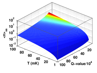
Fig. 3: (Color online) The final phonon number $\mathrm{log}\left\langle n\right\rangle_{ss}$ versus $Q$-value and environmental temperature T (mk), where we have $\omega_{m}=2\pi\times 1$ MHz, $\Omega_{0}=8\omega_{m}$, $\Delta=31\omega_{m}$, $\Gamma=15\omega_{m}$, and $\eta=0.115$ [30, 31, 34, 36, 38, 43].

We define a ratio $m_{R}=\Omega_{0}/\omega_{m}$, which means the Rabi frequency $\Omega_{0}$ increases with the increase of the ratio $m_{R}$. To have the largest cooling coefficient $A_{-}$, we choose $\Delta=(m_{R}^{2}-2)\omega_{m}/2$ which can ensure the transition $\left|d,n\right\rangle\rightarrow\left|+,n-1\right\rangle$ is resonant. Then we may rewrite the heating and cooling coefficients as

$$A_{+}=\eta^{2}\frac{2m_{R}^{2}\omega_{m}^{2}\Gamma}{4(m_{R}^{2}-2)^{2}\omega_{m}^{2}+\Gamma^{2}},~{}~{}~{}~{}~{}A_{-}=\eta^{2}\frac{2m_{R}^{2}\omega_{m}^{2}}{\Gamma},$$ (10)

which imply a hump curve in the heating coefficient and a parabolic curve for the cooling coefficient, as functions of $m_{R}$ [See Fig. 4(a)]. With assistance of Eqs. (3) and (4), these phenomena can be understood from the EIT cooling [26] as follows. Although the transition rates for both heating and cooling increase with the Rabi frequencies, the linewidth of the dressed state $\left|+\right\rangle$ decreases with the increase of detuning, and the states $\left|+,n-1\right\rangle$, $\left|+,n\right\rangle$ and $\left|+,n+1\right\rangle$ can be distinguished more clearly. Therefore, the red sideband transition between $\left|d,n\right\rangle$ and $\left|+,n-1\right\rangle$ is enhanced due to the resonance caused by the Rabi frequencies, and the carrier (blue sideband) transition between $\left|d,n\right\rangle$ and $\left|+,n\right\rangle$ ($\left|+,n+1\right\rangle$) is strongly suppressed by quantum interference. But the transition between $\left|d,n\right\rangle$ and $\left|+,n+1\right\rangle$ is enhanced first with the increase of Rabi frequencies, and then suppressed due to the detuning caused by the Rabi frequencies. As a result, the cooling coefficient is monotonically increasing, but the heating coefficient presents a hump with the increase of Rabi frequency.

Moreover, Fig. 4(a) also shows that the cooling rate $W=A_{-}-A_{+}$ is close to the cooling coefficient $A_{-}$ when $m_{R}\geq 8$ because the cooling coefficient is over ten times larger than the heating one in that case, e.g., the cooling coefficient $A_{-}=112.9$ kHz and the heating coefficient $A_{+}=1.6$ kHz if $m_{R}=8$.

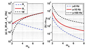
Fig. 4: (a) The cooling and heating coefficients $A_{\pm}$ and the cooling rate $W$ versus the ratio $m_{R}=\Omega_{0}/\omega_{m}$. Here the blue dotted, red solid, and black dashed lines correspond to the heating coefficient, cooling coefficient, and cooling rate, respectively. (b) The final average phonon number $\left\langle n\right\rangle_{ss}$ versus the ratio $m_{R}$. The parameters are taken from Refs. [30, 31, 34, 36, 38, 43] as $\omega_{m}=2\pi\times 1$ MHz, $\Gamma=15\omega_{m}$, $T=20$ mK and $\eta=0.115$.

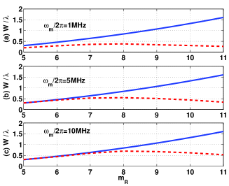
Fig. 5: The cooling $W$ in units of the magnetic coupling strength $\lambda$ versus the ratio $m_{R}=\Omega_{0}/\omega_{m}$. Here the blue red solid and red dashed lines correspond to the analytic cooling rate $W=A_{-}-A_{+}$ for Eq.(10) and the numerical cooling rate from the master equation for Eq.(2), respectively. And the frequency of the cantilever $\omega_{m}/2\pi$ in (a), (b), and (c) are 1MHz, 5MHz, and 10MHz. Here, $\Gamma/2\pi=15$MHz, $\lambda/2\pi=0.1$MHz.

It is worth mentioning that the adiabatic requirement $\Gamma\gg\lambda$ for deriving our analytical cooling rate formula Eq. (5) is always satisfied, due to the very large NV center excited state decay rate $\Gamma/(2\pi)=15$ MHz compared with the achievable value of $\lambda/(2\pi)=0.1$ MHz. It is interesting to notice that our analytical formula suggests that the cooling rate $W$ can exceed the NV-cantilever coupling strength $\lambda$ for sufficiently large optical Rabi frequency $\Omega_{0}$. We check whether this is true by plotting in Fig. 5 the cooling rate (obtained from direct numerical simulation of the coupled evolution) versus the Rabi frequency $\Omega_{0}$ for different cantilever frequencies $\omega_{m}$. Figure 5 shows that the maximal cooling rate is still limited by the coupling strength, e.g., $W\simeq 0.7\lambda$ ($0.55\lambda$, $0.38\lambda$) for the cantilever frequency $\omega_{m}/2\pi=10\$MHz (5 MHz, 1 MHz) and $\Omega_{0}=8\omega_{m}$. Nevertheness, the maximal cooling rate in the non-resolved sideband regime $\Gamma>\omega_{m}$ can be close to the coupling strength, e.g., $W\simeq 0.7\lambda$ at $\omega_{m}/2\pi=$10 MHz [see Fig. 5 (c)]. This is to be contrasted with Ref. [30]. There, efficient cooling is achieved in the resolved sideband regime and the cooling rate $W\simeq 0.8\lambda^{2}/\Gamma_{op}\ll 0.8\lambda$ due to the adiabatic requirement $\Gamma_{op}\gg\lambda$, i.e., the effective damping rate $\Gamma_{op}$ of the NV center should be much larger than the NV-cantilever coupling $\lambda$.

The corresponding final average phonon number as a function of the ratio $m_{R}$ is plotted in Fig. 4(b) for different cantilever decay $\gamma_{m}$, which is given by

$$\left\langle n\right\rangle_{ss}=\frac{\Gamma^{2}}{16[(m_{R}^{2}-2)/2\omega_{m}]^{2}}+N(\omega_{m})\frac{\gamma_{m}}{W}=\left(\frac{\Gamma}{4\Delta}\right)^{2}+N(\omega_{m})\frac{\gamma_{m}}{W}.$$ (11)

It means that the final average phonon number $\left\langle n\right\rangle_{ss}$ decreases with the increase of the detuning $\Delta$ for the fixed decay when the cooling coefficient $A_{-}$ takes its corresponding maximum value. Furthermore, Fig. 4(b) also shows that a lower final mean phonon number can be obtained by decreasing the cantilever decay rate. Besides, the equation for this cooling limit (11) is identical to the one in EIT cooling [25, 26, 28].

4 Simulation and Discussion

We have demonstrated in the above sections the possibility of the efficient optical EIT cooling for a cantilever attached with a NV center under the strong gradient magnetic field and laser fields. The cantilever can be cooled into its ground state by using the quantum interference and Zeeman effect. In the following, we will give some simulations to discuss how the scheme works in a realistic system.

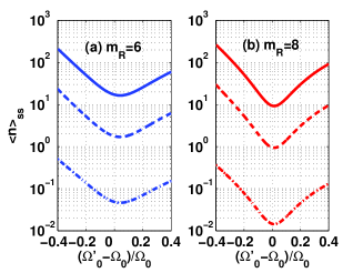
Fig. 6: The final average phonon number $\langle n\rangle_{ss}$ as a function of the variations around the optimal Rabi frequency $\Omega_{0}=m_{R}\omega_{m}$ with the detuning $\Delta=(m_{R}^{2}-2)\omega_{m}/2$. The simulation is made by Eq.(9), where $\omega_{m}=2\pi\times 1$MHz, $\Gamma=15\omega_{m}$, $T=20$mK, $\eta=0.115$ [30, 31, 34, 36, 38, 43]. The dash line, dot-dash line and solid line correspond to $\gamma_{m}=0$ Hz, $\gamma_{m}=10$ Hz, and $\gamma_{m}=100$ Hz, respectively.

To understand how the scheme works in a realistic system with the influence of the Rabi frequency, we plot in Fig. 6 the final phonon number by introducing fluctuation in the Rabi frequency $\Omega_{0}$. Here, we choose the parameters from the experimentally achievable constants in nano-mechanics [30, 31, 36, 38] as follows: $\omega_{m}=\mathrm{2\pi\times 1}$ MHz, $\Gamma=\mathrm{15\omega}_{m}$, $T=\mathrm{20}$ mK and $\eta=0.115$, and $Q=10^{5}$. All these parameters meet the approximation conditions mentioned above.

Figure 6 shows that the minimum value of the final average phonon number deviates from the point of $\Omega_{0}^{\prime}=\Omega_{0}$. This is due to the fact that the ideal cooling in our scheme depends on maximum value of $A_{-}$, rather than the maximum value of $A_{-}/A_{+}$. Moreover, Fig. 6 also shows that the final average phonon number is more sensitive to the experimental error in the case of the larger Rabi frequency since in this case the small deviation yields a large detuning if $(\Omega_{0}^{\prime}-\Omega_{0})/\Omega_{0}$ is ascertained.

As a result, to cool the cantilever down to its vibrational ground state, we must elaborately control the experimental imperfection in implementing our scheme. In addition, since the cantilever is sensitive to the environment, particularly for the small frequency cantilever, we have to remain the cooling by keeping irradiation from the external light fields.

Moreover, it is worth to point out that the nuclear spin bath gives a considerable influence on the final average phonon number and cooling time. For example, under the parameters with $\langle n\rangle_{initial}=20$, $m_{R}=8$ and $\gamma=$10Hz as in Fig. 6, the final average phonon number is increased from $\left\langle n\right\rangle_{ss}=$0.955 to $\left\langle n\right\rangle_{ss}=$1.111 (10.576) when the nuclear spin bath takes the random energy $\delta_{n}\leq 2\pi\times$ 0.1 MHz (0.5 MHz). The corresponding cooling time is increased from $t=0.547ms$ to $t=0.642ms(4.317ms)$, respectively. To decrease the impact of the nuclear spin bath, we should use the dynamic nuclear polarization technology [44] and the isotopic purification of NV center [45] to overcome this problem.

5 Conclusion

In summary, we have presented a protocol to cool the cantilever with a NV center attached down to the vibrational ground state under the strong MFG and laser fields. During the cooling process, the heating effects caused by the carrier transition and the blue sideband transition can be suppressed by quantum interference, and the cooling effects caused by the red sideband can be enhanced by increasing Rabi frequencies. We have shown the possibility of our scheme to cool the cantilever close to its ground state by controlling experimental imperfection. This implies that our scheme is a good candidate to realize the fast ground state cooling of cantilevers. In addition, we have also proven that our efficient optical EIT cooling proposal can be reduced to the EIT cooling one under some special conditions.

Appendix A

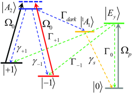
Fig. 7: The pumping process and the decays of NV center. The transition from state $|0\rangle$ and state $|E_{y}\rangle$ is driven by the pumping light $\Omega_{p}$. Here $\gamma_{\pm 1}$ and $\Gamma_{dark}$ are the direct decays from the excited state $|A_{2}\rangle$ to the ground states $|\pm 1\rangle$ and the metastable state $|^{1}A_{1}\rangle$, respectively. $\Gamma_{\pm 1}$ and $\Gamma_{0}$ are the direct decays from the excited state $|E_{y}\rangle$ to the ground states $|\pm 1\rangle$ and $|0\rangle$, respectively, while $\Gamma_{op}^{\pm 1}$ is the indirect decay from the state $|0\rangle$ to the state $|\pm 1\rangle$. $\gamma_{s}$ is the decay from the state $|S\rangle$ to the state $|0\rangle$.

As it is shown in Fig. 7, the state of the NV center $|A_{2}\rangle$ can decay to the state $|0\rangle$ with dark transition [35], which gives neither heating nor cooling to the cantilever. However, our cooling process will be stopped after the NV center is in the state $|0\rangle$. To avoid suspension of the cooling process, we will apply an additional pumping light on the transition from the state $|0\rangle$ to the state $|E_{y}\rangle$. This pumping process can not only realize a indirect transition from the state $|A_{2}\rangle$ to the state $|\pm 1\rangle$, but also give an effective decay to this indirect transition.

The pumping four-level systems are present in the right-hand side in Fig. 7, which start from the state $|0\rangle$ to the excited state $|E_{y}\rangle$, and then to the state $|\pm 1\rangle$ or $|0\rangle$. The decay processes for the final state $|\pm 1\rangle$ and $|0\rangle$ are corresponding to the effective decay process and dephasing process, respectively. Then, the Hamiltonian describes the pumping process can be given as ($\hbar=1$),

$$H_{p}=\omega_{e}\left|E_{y}\right\rangle\left\langle E_{y}\right|+\omega_{+1}\left|+1\right\rangle\left\langle+1\right|+\omega_{-1}\left|-1\right\rangle\left\langle-1\right|+\Omega_{p}(\left|E_{y}\right\rangle\left\langle 0\right|+\left|E_{y}\right\rangle\left\langle 0\right|)\cos(\omega_{p}t),$$ (12)

where the first three items describe the free energy for the NV center with $\omega_{e}$ and $\omega_{\pm 1}$ being the energy for states $\left|E_{y}\right\rangle$ and $\left|\pm 1\right\rangle$, respectively; the last item represents the transition between the states $\left|E_{y}\right\rangle$ and $\left|0\right\rangle$ driven by a pumping field with a Rabi frequency $\Omega_{p}$ and frequency $\omega_{p}$.

According to the effective operator formalism for open quantum system [46], we can calculate the effective decays as follows.

In the rotating frame of the pumping field frequency $\omega_{p}$, the above Hamiltonian can be rewritten as

$$\begin{array}[]{llllll}H_{p}&=&H_{e}+H_{g}+V_{-}+V_{+},&&&\\ H_{e}&=&\Delta_{e}\left|E_{y}\right\rangle\left\langle E_{y}\right|,&H_{g}&=&\omega_{\pm 1}\left|\pm 1\right\rangle\left\langle\pm 1\right|,\\ V_{-}&=&\frac{\Omega_{p}}{2}\left|0\right\rangle\left\langle E_{y}\right|,&V_{+}&=&\frac{\Omega_{p}}{2}\left|E_{y}\right\rangle\left\langle 0\right|\end{array}$$ (13)

with $\Delta_{e}=\omega_{e}-\omega_{p}$.

Then the non-Hermitian Hamiltonian for the quantum jump formalism is

$$H_{NH}=H_{e}-\frac{i}{2}(\Gamma_{0}+\Gamma_{-1}+\Gamma_{+1})(|E_{y}\rangle\langle E_{y}|).$$ (14)

And the corresponding effective Hamiltonian and Lindblad operators can be given as:

$$\begin{array}[]{lll}H_{eff}&=&-\frac{1}{2}V_{-}[H_{NV}^{-1}+(H_{NV}^{-1})^{{\dagger}}]V_{+}+H_{g}\\ &=&-\frac{\Delta_{e}\Omega_{p}^{2}}{4\Delta_{e}^{2}+(\Gamma_{0}+\Gamma_{-1}+\Gamma_{+1})^{2}}\left|0\right\rangle\left\langle 0\right|+\omega_{\pm 1}\left|\pm 1\right\rangle\left\langle\pm 1\right|;\\ L_{op}^{k}&=&L_{k}H_{NV}^{-1}V_{+},L_{k}=\sqrt{\Gamma_{k}}\left|k\right\rangle\left\langle E_{y}\right|;\\ L_{op}^{0}&=&\sqrt{\Gamma_{0}}\left|0\right\rangle\left\langle E_{y}\right|\frac{\left|E_{y}\right\rangle\left\langle E_{y}\right|}{\Delta_{e}-i\frac{1}{2}(\Gamma_{0}+\Gamma_{-1}+\Gamma_{+1})}\frac{\Omega_{p}}{2}\left|E_{y}\right\rangle\left\langle 0\right|\\ &=&\sqrt{\Gamma_{0}}\frac{1}{\Delta_{e}-i\frac{1}{2}(\Gamma_{0}+\Gamma_{-1}+\Gamma_{+1})}\frac{\Omega_{p}}{2}\left|0\right\rangle\left\langle 0\right|;\\ L_{op^{\pm 1}}&=&\sqrt{\Gamma_{\pm 1}}\left|\pm 1\right\rangle\left\langle E_{y}\right|\frac{\left|E_{y}\right\rangle\left\langle E_{y}\right|}{\Delta_{e}-i\frac{1}{2}(\Gamma_{0}+\Gamma_{-1}+\Gamma_{+1})}\frac{\Omega_{p}}{2}\left|E_{y}\right\rangle\left\langle 0\right|\\ &=&\sqrt{\Gamma_{\pm 1}}\frac{1}{\Delta_{e}-i\frac{1}{2}(\Gamma_{0}+\Gamma_{-1}+\Gamma_{+1})}\frac{\Omega_{p}}{2}\left|\pm 1\right\rangle\left\langle 0\right|.\end{array}$$ (15)

Here, $\Gamma_{0}$ ($\Gamma_{\pm 1}$) is the decay from the excited state $\left|E_{y}\right\rangle$ to the ground state $|0\rangle$ ($\left|\pm 1\right\rangle$).

As a result, the effective decay $L_{op}^{\pm 1}$ generates the ground state $\left|\pm 1\right\rangle$ from $\left|0\right\rangle$ can be reduced by

$$\begin{array}[]{lll}\Gamma_{op}^{\pm 1}&=&|\left\langle\pm 1\right|\sqrt{\Gamma_{\pm 1}}\frac{1}{\Delta_{e}-i\frac{1}{2}(\Gamma_{0}+\Gamma_{-1}+\Gamma_{+1})}\frac{\Omega_{p}}{2}\left|\pm 1\right\rangle\left\langle 0\right|\left|0\right\rangle|^{2}\\ &=&\Gamma_{\pm 1}\frac{\Omega_{p}^{2}}{4\Delta_{e}^{2}+(\Gamma_{0}+\Gamma_{-1}+\Gamma_{+1})^{2}}.\end{array}$$ (16)

and the dephasing of $\left|0\right\rangle$ can be written as

$$\begin{array}[]{lll}\Gamma_{op}^{0}&=&|\left\langle 0\right|\sqrt{\Gamma_{0}}\frac{1}{\Delta_{e}-i\frac{1}{2}(\Gamma_{0}+\Gamma_{-1}+\Gamma_{+1})}\frac{\Omega_{p}}{2}\left|0\right\rangle\left\langle 0\right|\left|0\right\rangle|^{2}\\ &=&\Gamma_{0}\frac{\Omega_{p}^{2}}{4\Delta_{e}^{2}+(\Gamma_{0}+\Gamma_{-1}+\Gamma_{+1})^{2}}.\end{array}$$ (17)

It is worth to point out that, $\Gamma_{op}^{+1}+\Gamma_{op}^{-1}+\Gamma_{op}^{0}$ can’t be larger than the decay for dark transition $\gamma_{0}=\Gamma-\gamma_{+1}-\gamma_{-1}$ from the state $|A_{2}\rangle$ to the state $|^{1}A_{1}\rangle$, and then to the state $\left|0\right\rangle$, since both the effective decay and dephasing are original from this dark transition process. Moreover, we can also define the real decay from the excited state $\left|A_{2}\right\rangle$ to the ground state $\left|\pm 1\right\rangle$ as $\gamma_{\pm}=\gamma_{\pm 1}+\Gamma_{op}^{\pm 1}$ with $\gamma_{\pm 1}$ being the direct decay from $\left|A_{2}\right\rangle$ to $\left|\pm 1\right\rangle$, and $\gamma_{+}+\gamma_{-}\leq\Gamma$. Considering the decay of dark transition is small, for simplicity, we assume $\gamma_{+}+\gamma_{-}\simeq\Gamma$ and use $\gamma_{\pm}$ to represent all the decays from the excited state $|A_{2}\rangle$ to the ground state $|\pm 1\rangle$.

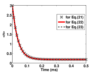
Fig. 8: The average phonon number $\langle n\rangle$ as a function of the time $T$. Assume the initial average phonon number is $\langle n\rangle=3$ and the NV center is in state $|-1\rangle$. The signs for crossing, the black dash line and red solid line are simulated with Eqs.(18), (19) and (20), respectively. Here $\omega_{m}=2\pi\times 1$MHz, $\Omega_{0}=6\omega_{m}$, $\Delta=10\omega_{m}$, $\Gamma=15\omega_{m}$, $\gamma_{\pm 1}=\Gamma/2$, $\Gamma_{dark}=\Gamma/130$, $\Gamma_{0}=\Gamma$, $\Gamma_{\pm 1}=\Gamma/150$, $\gamma_{s}=\Gamma/33$, $\gamma_{0}=0.1\Gamma$, $T=20$mK, $\eta=0.115$, $\Delta_{p}=0MHz$, and $\Omega_{p}=\Gamma$ [30, 31, 34, 36, 38, 43, 34, 35].

To check the accuracy of the real decays, we simulate the average phonon number $\left\langle n\right\rangle=Tr(b^{\dagger}b\rho)$ versus the time $T$ in Fig. 8 with and without the state $|0\rangle$. The corresponding master equations for the density matrix $\rho$ without and with the state $|0\rangle$, and the one for the real system are:

$$\begin{array}[]{lll}\frac{d}{dt}\rho&=&-i[H^{\mathrm{rot}},\rho]+\frac{\gamma_{m}}{2}[b\rho b^{\dagger}-\rho b^{\dagger}b-b^{\dagger}b\rho]\\ &+&\sum\limits_{{}_{\pm}}\frac{\gamma_{\pm}}{2}[\left|\pm 1\right\rangle\left\langle A_{2}\right|\rho\left|A_{2}\right\rangle\left\langle\pm 1\right|-\rho\left|A_{2}\right\rangle\left\langle A_{2}\right|-\left|A_{2}\right\rangle\left\langle A_{2}\right|\rho],\end{array}$$ (18)

$$\begin{array}[]{lll}\frac{d}{dt}\rho&=&-i[H^{\mathrm{rot}}-\omega_{0}\left|0\right\rangle\left\langle 0\right|,\rho]+\frac{\gamma_{m}}{2}[b\rho b^{\dagger}-\rho b^{\dagger}b-b^{\dagger}b\rho]\\ &+&\sum\limits_{{}_{\pm}}\frac{\gamma_{\pm 1}}{2}[\left|\pm 1\right\rangle\left\langle A_{2}\right|\rho\left|A_{2}\right\rangle\left\langle\pm 1\right|-\rho\left|A_{2}\right\rangle\left\langle A_{2}\right|-\left|A_{2}\right\rangle\left\langle A_{2}\right|\rho]\\ &+&\frac{\gamma_{0}}{2}[\left|0\right\rangle\left\langle A_{2}\right|\rho\left|A_{2}\right\rangle\left\langle 0\right|-\rho\left|A_{2}\right\rangle\left\langle A_{2}\right|-\left|A_{2}\right\rangle\left\langle A_{2}\right|\rho]\\ &+&\sum\limits_{{}_{\pm}}\frac{\Gamma_{op}^{\pm 1}}{2}[\left|\pm 1\right\rangle\left\langle 0\right|\rho\left|0\right\rangle\left\langle\pm 1\right|-\rho\left|0\right\rangle\left\langle 0\right|-\left|0\right\rangle\left\langle 0\right|\rho],\end{array}$$ (19)

and

$$\begin{array}[]{lll}\frac{d}{dt}\rho&=&-i[H^{\mathrm{rot}}-\omega_{s}\left|{}^{1}A_{1}\right\rangle\left\langle{}^{1}A_{1}\right|+\Omega_{p}(\left|E_{y}\right\rangle\left\langle 0\right|+\left|0\right\rangle\left\langle E_{y}\right|),\rho]\\ &+&\frac{\gamma_{m}}{2}[b\rho b^{\dagger}-\rho b^{\dagger}b-b^{\dagger}b\rho]\\ &+&\sum\limits_{{}_{\pm}}\frac{\gamma_{\pm 1}}{2}[\left|\pm 1\right\rangle\left\langle A_{2}\right|\rho\left|A_{2}\right\rangle\left\langle\pm 1\right|-\rho\left|A_{2}\right\rangle\left\langle A_{2}\right|-\left|A_{2}\right\rangle\left\langle A_{2}\right|\rho]\\ &+&\frac{\Gamma_{dark}}{2}[\left|{}^{1}A_{1}\right\rangle\left\langle A_{2}\right|\rho\left|A_{2}\right\rangle\left\langle{}^{1}A_{1}\right|-\rho\left|A_{2}\right\rangle\left\langle A_{2}\right|-\left|A_{2}\right\rangle\left\langle A_{2}\right|\rho]\\ &+&\frac{\gamma_{s}}{2}[\left|0\right\rangle\left\langle{}^{1}A_{1}\right|\rho\left|{}^{1}A_{1}\right\rangle\left\langle 0\right|-\rho\left|{}^{1}A_{1}\right\rangle\left\langle{}^{1}A_{1}\right|-\left|{}^{1}A_{1}\right\rangle\left\langle{}^{1}A_{1}\right|\rho],\\ &+&\frac{\Gamma_{0}}{2}[\left|0\right\rangle\left\langle E_{y}\right|\rho\left|E_{y}\right\rangle\left\langle 0\right|-\rho\left|E_{y}\right\rangle\left\langle E_{y}\right|-\left|E_{y}\right\rangle\left\langle E_{y}\right|\rho],\\ &+&\sum\limits_{{}_{\pm}}\frac{\Gamma_{\pm 1}}{2}[\left|\pm 1\right\rangle\left\langle E_{y}\right|\rho\left|E_{y}\right\rangle\left\langle\pm 1\right|-\rho\left|E_{y}\right\rangle\left\langle E_{y}\right|-\left|E_{y}\right\rangle\left\langle E_{y}\right|\rho],\end{array}$$ (20)

respectively. The last term in Eq.(19) describes the effective decay process from the state $\left|0\right\rangle$ to the state $\left|\pm 1\right\rangle$, which is caused by the pumping process. Here, $\gamma_{0}$ ($\gamma_{\pm 1}$, $\Gamma_{dark}$) is the decay from the excited state $\left|A_{2}\right\rangle$ to the state $\left|0\right\rangle$ ($\left|\pm 1\right\rangle$, $\left|{}^{1}A_{1}\right\rangle$) , $\Gamma_{0}$ ($\Gamma_{\pm 1}$) is the decay from the excited state $\left|E_{y}\right\rangle$ to the ground state $\left|0\right\rangle$ ($\left|\pm 1\right\rangle$), $\gamma_{s}$ is the decay from the state $\left|{}^{1}A_{1}\right\rangle$ to the ground state $\left|0\right\rangle$.

Compared with the simulation results, we find that the average phonon number $\left\langle n\right\rangle=Tr(b^{\dagger}b\rho)$ versus the time $T$ with Eqs.(18) (19) and (20) agree with each other very well since the decay from $\left|A_{2}\right\rangle$ to the state $\left|{}^{1}A_{1}\right\rangle$ is very small, the three-level system constitued by states $\left|A_{2}\right\rangle$ and $\left|\pm 1\right\rangle$ can be treated as a nearly closed three-level system. As a result, the real decay of our model is valid.

Appendix B

In what follows, we treat the coupling $V$ between the NV center and the cantilever by perturbation theory and use the non-equilibrium fluctuation-dissipation relation to derive the cooling and heating rates.

Defining operators $c=-ib$, $c^{\dagger}=ib^{\dagger}$ in Eq. (3), we can get $\left\langle b^{\dagger}b\right\rangle=\left\langle c^{\dagger}c\right\rangle$. After the position operator $X=x_{0}(c+c^{\dagger})$ introduced, we rewrite the interaction Hamiltonian (4) as

$$V=-\frac{i\eta}{x_{0}}X(\frac{\Omega_{0}}{\sqrt{2}}|A_{2}\rangle\langle d|-h.c.),$$ (21)

and the corresponding fluctuation spectrum is [47]

$$S(\omega)=\frac{1}{2M\omega_{m}}\int_{0}^{\infty}\mathrm{dt}e^{i\omega t}\langle F(t)F(0)\rangle_{ss},$$ (22)

where the notation $\langle\cdots\rangle_{ss}$ stands for the average value in atomic steady state $\rho_{ss}$ in the absence of cantilever and the Heisenberg operator $F(t)$ takes the form of

$$F(t)=-\frac{d}{dX}V\mid_{X=0}=\frac{i\eta}{\sqrt{2}x_{0}}(\Omega_{0}|A_{2}\rangle\langle d|-h.c.)=-\frac{\eta}{\sqrt{2}x_{0}}\Omega_{0}\sigma_{y}^{A_{2},d}.$$ (23)

Here $\sigma_{x}^{m,n}=|m\rangle\langle n|+|n\rangle\langle m|$ and $\sigma_{y}^{m,n}=-i(|m\rangle\langle n|-|n\rangle\langle m|)$ with $m,n=A_{2},\pm 1$.

The steady state for the NV center $\rho_{ss}$ can be obtained from the Bloch equation for Hamiltonian (3) and can be given as [47],

$$\begin{array}[]{ccl}\frac{d\left\langle\rho^{bb}\right\rangle}{dt}&=&-\frac{\sqrt{2}\Omega_{0}}{2}\left\langle\sigma_{y}^{A_{2},b}\right\rangle+\Gamma_{b}(1-\left\langle\rho^{bb}\right\rangle-\left\langle\rho^{dd}\right\rangle),\\ \frac{d\left\langle\rho^{dd}\right\rangle}{dt}&=&\Gamma_{d}(1-\left\langle\rho^{bb}\right\rangle-\left\langle\rho^{dd}\right\rangle),\\ \frac{d\left\langle\sigma_{x}^{bd}\right\rangle}{dt}&=&-\frac{\sqrt{2}\Omega_{0}}{2}\left\langle\sigma_{y}^{A_{2},d}\right\rangle,\\ \frac{d\left\langle\sigma_{y}^{bd}\right\rangle}{dt}&=&\frac{\sqrt{2}\Omega_{0}}{2}\left\langle\sigma_{x}^{A_{2},d}\right\rangle,\\ \frac{d\left\langle\sigma_{x}^{A_{2},b}\right\rangle}{dt}&=&-\frac{\Gamma}{2}\left\langle\sigma_{x}^{A_{2},b}\right\rangle+\Delta\left\langle\sigma_{y}^{A_{2},b}\right\rangle,\\ \frac{d\left\langle\sigma_{y}^{A_{2},b}\right\rangle}{dt}&=&-\frac{\Gamma}{2}\left\langle\sigma_{y}^{A_{2},b}\right\rangle-\sqrt{2}\Omega_{0}(2\left\langle\rho^{bb}\right\rangle+\left\langle\rho^{dd}\right\rangle-1)-\Delta\left\langle\sigma_{x}^{A_{2},b}\right\rangle,\\ \frac{d\left\langle\sigma_{x}^{A_{2},d}\right\rangle}{dt}&=&-\frac{\Gamma}{2}\left\langle\sigma_{x}^{A_{2},d}\right\rangle-\frac{\sqrt{2}\Omega_{0}}{2}\left\langle\sigma_{y}^{bd}\right\rangle+\Delta\left\langle\sigma_{y}^{A_{2},d}\right\rangle,\\ \frac{d\left\langle\sigma_{y}^{A_{2},d}\right\rangle}{dt}&=&-\frac{\Gamma}{2}\left\langle\sigma_{y}^{A_{2},d}\right\rangle+\frac{\sqrt{2}\Omega_{0}}{2}\left\langle\sigma_{x}^{bd}\right\rangle-\Delta\left\langle\sigma_{x}^{A_{2},d}\right\rangle,\end{array}$$ (24)

where $\gamma_{+}$, $\gamma_{-}$, $\Gamma_{d}=$ $\Gamma_{b}=(\gamma_{+}+\gamma_{-})/2$ are the decay rates for the excited state $|A_{2}\rangle$ to the states $|+1\rangle$, $|-1\rangle$, $|d\rangle$, and $|b\rangle$, respectively; $\Gamma=\gamma_{+}+\gamma_{-}$ is the total decay rate; $\rho_{bb}=|b\rangle\langle b|$, $\rho_{dd}=|d\rangle\langle d|$. The steady state for this Bloch equation is $\rho_{ss}=\rho^{dd}$, which means the steady state for the NV center is in a dark state.

When the NV center is in its dark state, since only $\left\langle\sigma_{y}^{A_{2},d}(t)\sigma_{y}^{A_{2},d}(0)\right\rangle_{ss}\neq 0$, the fluctuation spectrum is reduced to

$$S(\omega)=\eta^{2}(\frac{\Omega_{0}}{\sqrt{2}})^{2}\int_{0}^{\infty}\mathrm{dt}e^{i\omega t}\langle\sigma_{y}^{A_{2},d}(t)\sigma_{y}^{A_{2},d}(0)\rangle_{ss}.$$ (25)

According to the quantum regression theorem [47], the equation of the correlation functions can be written as

$$\begin{array}[]{ccl}\frac{d\left\langle\rho^{bb}(t)\sigma_{y}^{A_{2},d}(0)\right\rangle_{ss}}{dt}&=&-\frac{\sqrt{2}\Omega_{0}}{2}\left\langle\sigma_{y}^{A_{2},b}(t)\sigma_{y}^{A_{2},d}(0)\right\rangle_{ss}+\Gamma_{b}(\left\langle\sigma_{y}^{A_{2},d}\right\rangle_{ss}\\ &-&\left\langle\rho^{bb}(t)\sigma_{y}^{A_{2},d}(0)\right\rangle_{ss}-\left\langle\rho^{dd}(t)\sigma_{y}^{A_{2},d}(0)\right\rangle_{ss}),\\ \frac{d\left\langle\rho^{dd}(t)\sigma_{y}^{A_{2},d}(0)\right\rangle_{ss}}{dt}&=&\Gamma_{d}(\left\langle\sigma_{y}^{A_{2},d}\right\rangle_{ss}-\left\langle\rho^{bb}(t)\sigma_{y}^{A_{2},d}(0)\right\rangle_{ss}-\left\langle\rho^{dd}(t)\sigma_{y}^{A_{2},d}(0)\right\rangle_{ss}),\\ \frac{d\left\langle\sigma_{x}^{b,d}(t)\sigma_{y}^{A_{2},d}(0)\right\rangle_{ss}}{dt}&=&-\frac{\sqrt{2}\Omega_{0}}{2}\left\langle\sigma_{y}^{A_{2},d}(t)\sigma_{y}^{A_{2},d}(0)\right\rangle_{ss},\\ \frac{d\left\langle\sigma_{y}^{b,d}(t)\sigma_{y}^{A_{2},d}(0)\right\rangle_{ss}}{dt}&=&\frac{\sqrt{2}\Omega_{0}}{2}\left\langle\sigma_{x}^{A_{2},d}(t)\sigma_{y}^{A_{2},d}(0)\right\rangle_{ss},\\ \frac{d\left\langle\sigma_{x}^{A_{2},b}(t)\sigma_{y}^{A_{2},d}(0)\right\rangle_{ss}}{dt}&=&-\frac{\Gamma}{2}\left\langle\sigma_{x}^{A_{2},b}(t)\sigma_{y}^{A_{2},d}(0)\right\rangle_{ss}+\Delta\left\langle\sigma_{y}^{A_{2},b}(t)\sigma_{y}^{A_{2},d}(0)\right\rangle_{ss},\\ \frac{d\left\langle\sigma_{y}^{A_{2},b}(t)\sigma_{y}^{A_{2},d}(0)\right\rangle_{ss}}{dt}&=&-\frac{\Gamma}{2}\left\langle\sigma_{y}^{A_{2},b}(t)\sigma_{y}^{A_{2},d}(0)\right\rangle_{ss}+\sqrt{2}\Omega_{0}(2\left\langle\rho^{bb}(t)\sigma_{y}^{A_{2},d}(0)\right\rangle_{ss}\\ &+&\left\langle\rho^{dd}(t)\sigma_{y}^{A_{2},d}(0)\right\rangle_{ss}-\left\langle\sigma_{y}^{A_{2},d}\right\rangle_{ss})-\Delta\left\langle\sigma_{x}^{A_{2},b}(t)\sigma_{y}^{A_{2},d}(0)\right\rangle_{ss},\\ \frac{d\left\langle\sigma_{x}^{A_{2},d}(t)\sigma_{y}^{A_{2},d}(0)\right\rangle_{ss}}{dt}&=&-\frac{\Gamma}{2}\left\langle\sigma_{x}^{A_{2},d}(t)\sigma_{y}^{A_{2},d}(0)\right\rangle_{ss}-\frac{\sqrt{2}\Omega_{0}}{2}\left\langle\sigma_{y}^{b,d}(t)\sigma_{y}^{A_{2},d}(0)\right\rangle_{ss}\\ &+&\Delta\left\langle\sigma_{y}^{A_{2},d}(t)\sigma_{y}^{A_{2},d}(0)\right\rangle_{ss},\\ \frac{d\left\langle\sigma_{y}^{A_{2},d}(t)\sigma_{y}^{A_{2},d}(0)\right\rangle_{ss}}{dt}&=&-\frac{\Gamma}{2}\left\langle\sigma_{y}^{A_{2},d}(t)\sigma_{y}^{A_{2},d}(0)\right\rangle_{ss}+\frac{\sqrt{2}\Omega_{0}}{2}\left\langle\sigma_{x}^{b,d}(t)\sigma_{y}^{A_{2},d}(0)\right\rangle_{ss}\\ &-&\Delta\left\langle\sigma_{x}^{A_{2},d}(t)\sigma_{y}^{A_{2},d}(0)\right\rangle_{ss}.\end{array}$$ (26)

Define the transformation

$$f(t)\rightleftharpoons F(\nu)=\int_{0}^{\infty}\mathrm{dt}e^{i\nu t}f(t),$$ (27)

then

$$\frac{f(t)}{dt}\rightleftharpoons-f(0)-i\nu F(\nu).$$ (28)

After the equations above solved, we can obtain

$$\int_{0}^{\infty}\mathrm{dt}e^{i\omega t}\left\langle\sigma_{y}^{A_{2},d}(t)\sigma_{y}^{A_{2},d}(0)\right\rangle_{ss}=\frac{2i\omega}{i\Gamma\omega+2\Delta\omega+2\omega^{2}-\Omega_{0}^{2}}$$ (29)

and the corresponding heating (cooling) coefficient $A_{+}$ ($A_{-}$) as

$$A_{\pm} = 2\mathrm{Re}\{S(\mp\omega_{m})\}$$ (30)

$$= 2\Gamma\eta^{2}\Omega_{0}^{2}\frac{\omega_{m}^{2}}{\Gamma^{2}\omega_{m}^{2}+4[\frac{\Omega_{0}^{2}}{2}\pm\Delta\omega_{m}-\omega_{m}^{2}]^{2}}.$$