Large-scale MU-MIMO: It Is Necessary to Deploy Extra Antennas at Base Station

Abstract

In this paper, the large-scale MU-MIMO system is considered where a base station (BS) with extremely large number of antennas ($N$) serves relatively less number of users ($K$). In order to achieve largest sum rate, it is proven that the amount of users must be limited such that the number of antennas at the BS is preponderant over that of the antennas at all the users. In other words, the antennas at the BS should be excess. The extra antennas at the BS are no longer just an optional approach to enhance the system performance but the prerequisite to the largest sum rate. Based on this factor, for a fixed $N$, the optimal $K$ that maximizes the sum rate is further obtained. Additionally, it is also pointed out that the sum rate can be substantially improved by only adding a few antennas at the BS when the system is $N=KM$ with $M$ denoting the antennas at each user. The derivations are under the assumption of $N$ and $M$ going to infinity, and being implemented on different precoders. Numerical simulations verify the tightness and accuracy of our asymptotic results even for small $N$ and $M$.

I Introduction

Large-scale multiuser multiple-input multiple-output (LS MU-MIMO) systems are currently regarded as a novel communication architecture. By exploiting extremely large number of antennas ($N$) at the base bastion (BS) to serve relatively less number of users ($K$), several attractive advantages are emerged, such as the increased system capacity, the reduced power consumption, and the improved spectral efficiency[1, 2, 3]. Therefore, the extra antennas at the BS are regarded as an optional approach to enhance the system performance.

However, with such large transmit dimensions (created by $N$), it is intuitional to serve the same scale of users for larger sum rate. But, as shown in this paper, the sum rate decreases instead of increasing with $K$ if the transmit power at the BS is not sufficiently large after a certain number of users. Consequently, it is requisite to keep the transmit dimensions excess for the largest sum rate as well.

This fact is caused by the existence of the multiuser interference (MUI). Since that the optimal approach to pre-cancel the MUI, the dirty-paper coding (DPC), is too complex to be implemented, simple linear precoders are chosen as the only option for LS MU-MIMO systems [3]. While, those linear precoders consumes the transmit dimensions when they null out the MUI. Hence, the more users are served, the less transmit dimensions for each user are left. As a result, if the transmit power is not large enough to compensate for the loss of transmit dimensions for each user, the sum rate is declined.

Hence, unlike the previous works treating the extra transmit dimensions as an optional approach to improve the system performance, our contributions in this paper are that the excess of antennas at the BS is proven to be a prerequisite to the largest sum rate as well.

More specifically, if $N$ is fixed, it is proven that the largest sum rate occurs at a certain $K$ where $N$ is greater than the amount of antennas at all $K$ users. Subsequently, the optimal $K$ that maximizes the sum rate is further obtained for a given $N$. Though similar works can be found in [4] and [5], their works are only focused on the zero-forcing (ZF) precoders for LS MU multiple-input single-output (LS MU-MISO) systems where $N$ is much larger than $K$, which can be included as a special case of our works. Additionally, it is shown that making the system in $N=KM$ with $M$ denoting the antennas at each user is always not the optimal strategy, the sum rate can be substantially improved by only adding a few antennas at the BS. The derivations are under the assumption of large-scale systems, and being implemented on the ZF precoders, the regularized ZF (RZF) precoders, and the singular value decomposition (SVD)-based precoders, respectively. As shown by numerical simulations, the our results are proven to be asymptotically tight and accurate for the systems with realistic dimensions.

Notions: Throughout this paper, vectors and matrices are denoted by boldface letters. $\left(\cdot\right)^{H}$, $\left(\cdot\right)^{\dagger}$, $\mathrm{tr}\left(\cdot\right)$, $\mathrm{E}\left[\cdot\right]$, and $\left\lfloor\cdot\right\rfloor$ denote conjugate transposition, pseudo-inversion, trace, the expectation, and round down operation, respectively. Furthermore, ‘$a.s.$’ means almost surely, and $\left(x\right)^{+}=\max\left(0,x\right)$. The $n$-dimension identity matrix is donated as $\boldsymbol{\mathrm{I}}_{n}$. $\log$ denotes the logarithm to the base of $2$.

II System Model

Consider a single-cell downlink MU-MIMO system in Fig. 1,

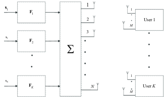
Figure 1: System model for LS MU-MIMO system

which comprises of a central BS with $N$ antennas and $K$ uncooperative users with $M$ antennas. $N\geq KM$ is preferred, thus, user scheduling is not taken into account.The received signal for the $k$-th user is given by

$$\boldsymbol{\mathrm{y}}_{k}=\boldsymbol{\mathrm{H}}_{k}\boldsymbol{\mathrm{F}}_{k}\boldsymbol{\mathrm{s}}_{k}+\boldsymbol{\mathrm{H}}_{k}\sum_{l\neq k}^{K}\boldsymbol{\mathrm{F}}_{l}\boldsymbol{\mathrm{s}}_{k}+\boldsymbol{\mathrm{n}}_{k},$$ (1)

where $\boldsymbol{\mathrm{y}}_{k}\in\mathbb{C}^{M\times 1}$, $\boldsymbol{\mathrm{s}}_{k}\in\mathbb{C}^{M\times 1}$, $\boldsymbol{\mathrm{H}}_{k}\in\mathbb{C}^{M\times N}$, $\boldsymbol{\mathrm{F}}_{k}\in\mathbb{C}^{N\times M}$, and $\boldsymbol{\mathrm{n}}_{k}\in\mathbb{C}^{M\times 1}$ are the received signal, information-bearing signal, channel matrix, precoder matrix, and Gaussian thermal noise vector for the $k$-th user, respectively. Since a LS-MIMO system is assumed, the entries of $\boldsymbol{\mathrm{H}}_{k}$ can be modeled as the identically independently distributed (i.i.d) circularly-symmetric complex Gaussian distribution with zero mean and variance $\sigma_{n}^{2}$, namely, $\mathcal{CN}\left(0,\sigma_{n}^{2}\right)$. For frequency selective fading channels, this model can be extended by using orthogonal frequency division multiplexing modulation (OFDM) [4]. The channel side information at transmitter (CSIT) is assumed.

Clearly, the transmit dimensions for the $k$-th user is $N$, but the current user suffers the MUI, namely, the second term of the right hand side (RHS) of (1). Hence, the precoding techniques are required to be utilized at the BS to pre-cancel the MUI.

The linear precoder are designed for single-user (SU) MIMO (SU-MIMO) systems, which can be extended to MU-MIMO systems by block diagonalization (BD) technique [6]. The precoder for BD technique is a cascade of two precoding matrices, namely, $\boldsymbol{\mathrm{F}}_{k}=\boldsymbol{\mathrm{B}}_{k}\boldsymbol{\mathrm{D}}_{k}$, where $\boldsymbol{\mathrm{B}}_{k}$ removes the MUI and $\boldsymbol{\mathrm{D}}_{k}$ can be further designed under the different criteria. To do so, $\boldsymbol{\mathrm{B}}_{k}$ should be chosen from the null space of $\boldsymbol{\mathrm{H}}_{l}$ ($\forall l\neq k$), i.e., $\boldsymbol{\mathrm{H}}_{l}\boldsymbol{\mathrm{B}}_{k}=\boldsymbol{\mathrm{0}}$ for any $l\neq k$. In particular, if $\tilde{\boldsymbol{\mathrm{H}}}_{k}$ is defined as $\tilde{\boldsymbol{\mathrm{H}}}_{k}=\left[\boldsymbol{\mathrm{H}}_{1}^{H},\dots,\boldsymbol{\mathrm{H}}_{k-1}^{H},\boldsymbol{\mathrm{H}}_{k+1}^{H},\dots,\boldsymbol{\mathrm{H}}_{K}^{H}\right]^{H}$, then $\boldsymbol{\mathrm{B}}_{k}$ can be obtained by the SVD on $\tilde{\boldsymbol{\mathrm{H}}}_{k}$, namely,

$$\tilde{\boldsymbol{\mathrm{H}}}_{k}=\tilde{\boldsymbol{\mathrm{U}}}_{k}\left[\tilde{\boldsymbol{\mathrm{\Sigma}}}_{k}\;\boldsymbol{\mathrm{0}}\right]\left[\tilde{\boldsymbol{\mathrm{V}}}_{k}^{\left(1\right)}\;\tilde{\boldsymbol{\mathrm{V}}}_{k}^{\left(0\right)}\right]^{H},$$

where $\tilde{\boldsymbol{\mathrm{U}}}_{k}$ and $\tilde{\boldsymbol{\mathrm{\Sigma}}}_{k}$ are the left singular vector matrix and the matrix of ordered singular values of $\tilde{\boldsymbol{\mathrm{H}}}_{k}$, respectively. Matrices $\tilde{\boldsymbol{\mathrm{V}}}_{k}^{\left(1\right)}$ and $\tilde{\boldsymbol{\mathrm{V}}}_{k}^{\left(0\right)}$ denote the right singular matrices, each of them consists of the singular vectors corresponding to non-zero singular values and zero singular values of $\tilde{\boldsymbol{\mathrm{H}}}_{k}$, respectively. Note that $\boldsymbol{\mathrm{H}}_{l}\tilde{\boldsymbol{\mathrm{V}}}_{k}^{\left(0\right)}=\boldsymbol{\mathrm{0}}$ ($\forall l\neq k$), $\boldsymbol{\mathrm{B}}_{k}$ is obtained by choosing $L_{k}$ columns from the $\tilde{\boldsymbol{\mathrm{V}}}_{k}^{\left(0\right)}$. To ensure there are at least $L_{k}$ columns in each $\tilde{\boldsymbol{\mathrm{V}}}_{k}^{\left(0\right)}$, $L_{k}$ should satisfy the dimensionality constraint as

$$L_{k}\leq N-\left(K-1\right)M.$$ (2)

Therefore, with $\boldsymbol{\mathrm{B}}_{k}$, (1) is rewritten as

$$\boldsymbol{\mathrm{y}}_{k}=\boldsymbol{\mathrm{H}}_{eq,k}\boldsymbol{\mathrm{D}}_{k}\boldsymbol{\mathrm{s}}_{k}+\boldsymbol{\mathrm{n}}_{k},$$ (3)

where $\boldsymbol{\mathrm{H}}_{eq,k}=\boldsymbol{\mathrm{H}}_{k}\boldsymbol{\mathrm{B}}_{k}\in\mathbb{C}^{M\times L_{k}}$ is the equivalent channel for $k$-th user. The transmission model in (3) can be interpreted as an equivalent SU-MIMO system in Fig. 2,

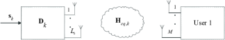
Figure 2: Equivalent system for each user

which a BS with $L_{k}$ antennas communicates with a receiver with $M$ antennas. $\boldsymbol{\mathrm{D}}_{k}\in\mathbb{C}^{L_{k}\times M}$ is therefore the precoder for such system. To ensure the existence of $\boldsymbol{\mathrm{D}}_{k}$, $L_{k}\geq M$ needs to be satisfied too.

Obviously, (3) does not suffer the MUI, but it is worth noticing that the transmit dimensions for each user have been declined from $N$ in (1) to $L_{k}$ in (3). The loss of transmit dimensions will definitely decrease the rate for the current user. However, due to the cancellation of the MUI, the entire LS MU-MIMO system achieves the full degrees of freedom (DoFs) promised by the DPC precoding. If the transmit power at the BS can enhance unlimitedly to compensate for the loss of transmit dimensions, the sum rate will increase with $K$. While, for the case of limited transmit power, there is tradeoff between the number of users and the transmit dimensions.

Define the sum rate of the MU-MIMO system using BD technique as

$$\mathcal{R}_{sum}=\sum_{k=1}^{K}\mathcal{R}_{k}$$ (4)

with

$$\mathcal{R}_{k}=\mathrm{E}\left\{\log\det\left(\boldsymbol{\mathrm{I}}_{M_{k}}+\frac{1}{\sigma_{n}^{2}}\boldsymbol{\mathrm{H}}_{eq,k}\boldsymbol{\mathrm{Q}}_{eq,k}\boldsymbol{\mathrm{H}}_{eq,k}^{H}\right)\right\},$$

where $\boldsymbol{\mathrm{Q}}_{eq,k}=\mathrm{E}\left[\boldsymbol{\mathrm{D}}_{k}\boldsymbol{\mathrm{D}}_{k}^{H}\right]$ denotes the input covariance matrix and the $\sigma_{n}^{2}$ is the variance of the noise. Since the transmit power is always limited, the following works in this paper is to quantify the impact of the tradeoff on $\mathcal{R}_{sum}$.

III Asymptotic Sum Rate of Different Precoders

In this section, the asymptotic sum rate performance of three different precoders is derived, as a groundwork of analysis in the next section. Before further introducing current section, a basic theorem is given at first.

Theorem: Consider two random matrices $\boldsymbol{\mathrm{A}}\in\mathbb{C}^{M\times N}$ and $\boldsymbol{\mathrm{B}}\in\mathbb{C}^{N\times L}$, where the entries in $\boldsymbol{\mathrm{A}}$ follow i.i.d $\mathcal{CN}\left(0,1\right)$ and $\boldsymbol{\mathrm{B}}^{H}\boldsymbol{\mathrm{B}}=\boldsymbol{\mathrm{I}}_{L}$. If $\boldsymbol{\mathrm{A}}$ is independent of $\boldsymbol{\mathrm{B}}$, the entries in $\boldsymbol{\mathrm{H}}=\boldsymbol{\mathrm{A}}\boldsymbol{\mathrm{B}}$ share the same distributions as those in $\boldsymbol{\mathrm{A}}$.

Proof:

See in [6], also in [7]. ∎

III-A Singular Value Decomposition-based Precoder

The principle of SVD-based precoder is to decompose the system channel into several parallel sub-channels, then implementing the power allocation using water-filling algorithm to make all the exploited sub-channels have the same gains.

Let $\boldsymbol{\mathrm{D}}_{k}=\boldsymbol{\mathrm{V}}_{k}\boldsymbol{\mathrm{M}}_{k}^{1/2}$, where $\boldsymbol{\mathrm{V}}_{k}$ is the right singular matrix of $\boldsymbol{\mathrm{H}}_{eq,k}$ and $\boldsymbol{\mathrm{M}}_{k}$ is the diagonal power allocation matrix. Assuming the transit power allocated to the $k$-th user is $P_{k}$, The principle of SVD-based precoder can be mathematically expressed as

$$\mathcal{R}_{k}^{SVD}=\mathrm{E}\left\{\sum_{i=1}^{M}\left[\log\left(M\nu\lambda_{i}\right)\right]^{+}\right\}$$

with the power level $\nu$ obtained from

$$\frac{1}{M}\sum_{i=1}^{M}\left(M\nu-\frac{1}{\lambda_{i}}\right)^{+}=\rho_{k},$$

where $\lambda_{i}$ denotes the $i$-th eigenvalue of $M^{-1}\boldsymbol{\mathrm{H}}_{eq,k}\boldsymbol{\mathrm{H}}_{eq,k}^{H}$ and $\rho_{k}=P_{k}/\sigma_{n}^{2}$.

Clearly, $\mathcal{R}_{k}^{SVD}$ depends on $\lambda_{i}$ ($i=1,\dots,M$). Since the distributions of eigenvalues for a matrix with regular dimensions are too complex to be further analyzed, the asymptotic behavior of $\lambda_{i}$ is mainly focused.

Based on the Theorem above, the entries in $\boldsymbol{\mathrm{H}}_{eq,k}$ follow the i.i.d zero-mean Gaussian distribution with unity variance. Thus, when $\rho_{k}\geq\frac{2}{\left(\sqrt{\beta_{k}}-1\right)\left(\beta_{k}-1\right)}$, $\mathcal{R}_{k}^{SVD}$ almost surely converges to a deterministic value as $L_{k},M\rightarrow\infty$ with $L_{k}/M\rightarrow\beta_{k}$ , namely,

$$\mathcal{R}_{k}^{SVD}\xrightarrow{a.s.}M\Big{[}\log\left(1+\rho_{k}\left(\beta_{k}-1\right)\right)+\beta_{k}\log\beta_{k}\\ -\beta_{k}\log\left(\beta_{k}-1\right)-\log e\Big{]},$$ (5)

where the derivation is directly based on [8] and the constraint on $\rho_{k}$ ensures all the sub-channels are exploited for data transmission.

(5) only holds in the case of $\beta_{k}>1$. For $\beta_{k}=1$, the minimum eigenvalue of $M^{-1}\boldsymbol{\mathrm{H}}_{eq,k}\boldsymbol{\mathrm{H}}_{eq,k}^{H}$, denoted by $\lambda_{\min}$, converges to zero under large-scale system assumption [9]. In this case, only part of the the sub-channels will be used. Under the circumstance, $\mathcal{R}_{k}^{SVD}$ shows almost sure convergence to

$$\mathcal{R}_{k}^{SVD}\xrightarrow{a.s.}\int_{\bar{\nu}^{-1}}^{4}\log_{2}\left(\bar{\nu}x\right)f_{1}\left(x\right)dx$$ (6)

with $\bar{\nu}=M\nu$ calculated from

$$\int_{\bar{\nu}^{-1}}^{4}\left(\bar{\nu}-\frac{1}{x}\right)f_{1}\left(x\right)dx=\rho_{k},$$ (7)

where $f_{1}\left(x\right)$ is the probability density of Marc̆enko-Pastur distribution with parameter one [10]. Solving the integral in (7) yields

$$\rho_{k}=\frac{1}{2\pi}\left[(1+2\bar{\nu})\arccos\left(\frac{1-2\bar{\nu}}{2\bar{\nu}}\right)-3\sqrt{4\bar{\nu}-1}\right].$$ (8)

Since the right hand side (RHS) in (8) is a monotonically increasing function of $\bar{\nu}$ in the region $\left[0.25,\infty\right)$, the solution is unique for every positive value of $\rho_{k}$. Subsequently, (6) can be calculated using numerical integral technique.

Similarly to the definition in (4), the asymptotic sum rate of SVD-based precoder, $\bar{\mathcal{R}}_{sum}^{SVD}$, can be obtained via (5) and (6) for different values of $\beta_{k}$.

III-B Zero-forcing Precoder

Unlike the SVD-based precoder decomposing the entire channel into several sub-channels, the ZF precoder ‘smoothes’ the channel by inversion operation, hence, the received signal is just a scaled version of information-bearing signal. Specifically, by defining $\boldsymbol{\mathrm{D}}_{k}=\kappa\boldsymbol{\mathrm{H}}_{eq,k}^{\dagger}$, the rate of $k$-th UT, $\mathcal{R}_{k}^{ZF}$, is revised as

$$\mathcal{R}_{k}^{ZF}=M\mathrm{E}\left\{\log\left(1+\kappa^{2}/\sigma_{n}^{2}\right)\right\},$$

in which $\kappa=\sqrt{P_{k}/\mathrm{tr}\left(\boldsymbol{\mathrm{D}}_{k}\boldsymbol{\mathrm{D}}_{k}^{H}\right)}$ is the power constraint factor. Clearly, $\kappa$ dominants the performance of $\mathcal{R}_{k}^{ZF}$. To have a friendly expression, the $\mathcal{R}_{k}^{ZF}$ is rewritten as

$$\mathcal{R}_{k}^{ZF} = M\mathrm{E}\left\{\log\left(1+\rho_{k}/\mathrm{tr}\left[\left(\boldsymbol{\mathrm{H}}_{eq,k}\boldsymbol{\mathrm{H}}_{eq,k}^{H}\right)^{-1}\right]\right)\right\},$$ (9)

$$\xrightarrow{a.s.} M\mathrm{E}\left\{\log\left(1+\rho_{k}\left(\beta_{k}-1\right)\right)\right\},$$

where the ‘$\xrightarrow{a.s.}$’ abides by the asymptotic behavior of $M^{-1}\boldsymbol{\mathrm{H}}_{eq,k}\boldsymbol{\mathrm{H}}_{eq,k}^{H}$ [4].

Obviously, (9) does not hold when $\beta_{k}$ approaches one. That is because that the $\lambda_{\min}$ will converge to zero with probability one in the case of $\beta_{k}=1$, the first order moment of $\left(\boldsymbol{\mathrm{H}}_{eq,k}\boldsymbol{\mathrm{H}}_{eq,k}^{H}\right)^{-1}$ is no longer converged.

In order to evaluate the asymptotic performance of $\mathcal{R}_{k}^{ZF}$ when $\beta_{k}$ equals one, the upper bound of $\mathcal{R}_{k}^{ZF}$ is derived, namely,

$$\mathcal{R}_{k}^{ZF} = M\mathrm{E}\left\{\log\left(1+\rho_{k}\left(M^{-1}\sum_{i=1}^{M}\lambda^{-1}\right)^{-1}\right)\right\},$$ (10)

$$\leq \mathrm{E}\left\{\sum_{i=1}^{M}\log\left(1+\rho_{k}\lambda_{i}\right)\right\},$$

where ‘$\leq$’ follows from Jensen’s inequality. The RHS of (10) converges to the following integral with probability one as $L_{k},M\rightarrow\infty$ with $L_{k}/M\rightarrow\beta$, i.e.,

$$\mathrm{E}\left\{\sum_{i=1}^{M}\log\left(1+\rho_{k}\lambda_{i}\right)\right\}\xrightarrow{a.s.}M\int\log\left(1+\rho_{k}x\right)f_{\beta_{k}}\left(x\right)dx,$$

in which $f_{\beta_{k}}\left(x\right)$ is the probability density of Marc̆enko-Pastur distribution with parameter $\beta_{k}$. The integral yields a closed-form solution, which is

$$\mathcal{R}_{k}^{ZF}\preccurlyeq M\Big{[}\beta_{k}\log\left(1+\rho_{k}-\mathcal{F}\left(\rho_{k},\beta_{k}\right)\right)\\ +\log\left(1+\rho_{k}\beta_{k}-\mathcal{F}\left(\rho_{k},\beta_{k}\right)\right)-\frac{\log e}{\rho_{k}}\mathcal{F}\left(\rho_{k},\beta_{k}\right)\Big{]},$$ (11)

where

$$\mathcal{F}\left(x,y\right)=\left(\sqrt{x\left(1+\sqrt{y}\right)^{2}+1}-\sqrt{x\left(1-\sqrt{y}\right)^{2}+1}\right)^{2}$$

and ‘$\preccurlyeq$’ denotes asymptotically equal or less than.

Consequently, the asymptotic sum rate of ZF precoder, $\bar{\mathcal{R}}_{sum}^{ZF}$, can be derived from (9) and (11) for by (4) for different values of $\beta_{k}$.

III-C Regularized Zero-forcing Precoder

The RZF precoder is proposed to improve the performance of ZF precoder in the case of $\beta_{k}=1$ by adding a multiple of the identify matrix before inversion, namely, $\boldsymbol{\mathrm{D}}_{k}=\kappa\boldsymbol{\mathrm{W}}\boldsymbol{\mathrm{H}}_{eq,k}^{H}$ with $\boldsymbol{\mathrm{W}}=\left(\boldsymbol{\mathrm{H}}_{eq,k}^{H}\boldsymbol{\mathrm{H}}_{eq,k}+M\rho_{k}^{-1}\boldsymbol{\mathrm{I}}_{L_{k}}\right)^{-1}$.

Unlike the previous precoders, the received signal suffers the inter-stream interference. Recalling the transmission model in (3), the $i$-th stream for the $k$-th user is given as

$$y_{i}=\kappa\boldsymbol{\mathrm{h}}_{i}\boldsymbol{\mathrm{W}}\boldsymbol{\mathrm{h}}_{i}^{H}s_{i}+\kappa\boldsymbol{\mathrm{h}}_{i}\sum_{j\neq i}^{M_{k}}\boldsymbol{\mathrm{W}}\boldsymbol{\mathrm{h}}_{j}^{H}s_{j}+n_{i},$$

where $\boldsymbol{\mathrm{h}}_{i}$ $y_{i}$, $s_{i}$, and $n_{i}$ denote the $i$-th row of $\boldsymbol{\mathrm{H}}_{eq,k}$, the $i$-th elements in $\boldsymbol{\mathrm{y}}_{k}$, $\boldsymbol{\mathrm{s}}_{k}$, and $\boldsymbol{\mathrm{n}}_{k}$, respectively. Hence, $\mathcal{R}_{k}^{RZF}$ is redefined as a function of received signal-to-noise-plus-interference-ratio (SINR) for each stream, i.e.,

$$\mathcal{R}_{k}^{RZF}=\mathrm{E}\left\{\sum_{i=1}^{M}\log\left(1+\gamma_{i}\right)\right\}$$

with the SINR for the $i$-th stream

$$\gamma_{i}=\frac{\left|\boldsymbol{\mathrm{h}}_{i}\boldsymbol{\mathrm{W}}\boldsymbol{\mathrm{h}}_{i}^{H}\right|^{2}}{\left(\boldsymbol{\mathrm{h}}_{i}\boldsymbol{\mathrm{W}}\boldsymbol{\mathrm{H}}_{\left[i\right]}^{H}\boldsymbol{\mathrm{H}}_{\left[i\right]}\boldsymbol{\mathrm{W}}\boldsymbol{\mathrm{h}}_{i}+\sigma_{n}^{2}/\kappa^{2}\right)},$$

where $\boldsymbol{\mathrm{H}}_{\left[i\right]}$ is the $\boldsymbol{\mathrm{H}}_{eq,k}$ with $i$-th row removed.

Before introducing the asymptotic behavior of $\mathcal{R}_{k}^{RZF}$, it is pointed out that the largest eigenvalue of $M^{-1}\boldsymbol{\mathrm{H}}_{eq,k}\boldsymbol{\mathrm{H}}_{eq,k}^{H}$, $\lambda_{\max}$, shows the almost sure convergence to a deterministic value as $L_{k},M\rightarrow\infty$ with $L_{k}/M\rightarrow\beta_{k}$, namely [9],

$$\lambda_{\max}\xrightarrow{a.s.}\left(1+\sqrt{\beta_{k}}\right)^{2}.$$

Therefore, $M^{-1}\boldsymbol{\mathrm{H}}_{eq,k}\boldsymbol{\mathrm{H}}_{eq,k}^{H}$ has uniformly bounded spectral norm on $M$ with probability one. Based on this fact, $\mathcal{R}_{k}^{RZF}$ converges to the following equation with the large-scale system assumption, i.e.,

$$\hskip 10.00002pt\mathcal{R}_{k}^{RZF}\xrightarrow{a.s.}M\Bigg{[}\log_{2}\Bigg{(}1+\rho_{k}\left(\beta_{k}-1\right)\\ +\sqrt{\rho_{k}^{2}\left(\beta_{k}-1\right)^{2}+2\rho_{k}\left(\beta_{k}+1\right)+1}\Bigg{)}-1\Bigg{]},$$ (12)

which is based on [5, Corollary 2].

Consequently, the asymptotic sum rate of RZF precoder, $\bar{\mathcal{R}}_{sum}^{RZF}$, is achievable by substituting (12) into (4).

IV Results and Numerical Simulations

In this section, the main results in this paper are presented, and being verified by numerical simulations. There is tradeoff between transmit dimensions and the number of users is given at first, followed by the optimal $K$ that maximizes the $\mathcal{R}_{sum}$.

Throughout this section, a $\left(N,M,K\right)$ system is referred as a $K$ users system with $N$ transmit antennas at the BS and $M$ receive antennas at each user. $L_{k}$ and $P_{k}$ are assumed to be $L=N-\left(K-1\right)M$ and $P$ for all the users. The assumption is logical, because the large transmit dimensions maximizes the rate per user, and it is unnecessary to implement power allocation among statistically identical users. Additionally, ‘ZF’, ‘RZF’, and ‘SVD’ are abbreviations for the MU-MIMO systems using BD technique with ZF precoder, RZF precoder, and SVD-based precoder, respectively.

Based on the configurations above, $\beta_{k}$ is further rewritten as

$$\beta_{k}=\beta-K+1,$$ (13)

where $\beta=N/M$ is the normalized the transmit dimensions. And $\rho_{k}$ is set to $\rho$ for all the user with $\rho=P/\sigma_{n}^{2}.$ Clearly, the normalized transmit dimensions per user ($\beta_{k}$) is declined with $K$.

To quantify the impact of the tradeoff on the sum rate, the asymptotic sum rates of above three different precoders is summarized into an unified form, donated by $\bar{\mathcal{R}}_{sum}$, namely,

$$\bar{\mathcal{R}}_{sum}\left(K,\rho\right)=KM\left[\mathcal{I}_{1}\left(K,\rho\right)+\mathcal{I}_{2}\left(K,\rho\right)\right],\;\text{for }K<\beta$$ (14)

where $\mathcal{I}_{1}\left(K,\rho\right)=\log\left(1+\rho\left(\beta-K\right)\right)$, and $\mathcal{I}_{2}\left(K,\rho\right)$ varies from different precoders whose explicit forms can be found in Table I.

Table I: Explicit forms of array gain for different precoders

	$\mathcal{I}_{2}\left(K,\rho\right)$
SVD	$\left(\beta-K+1\right)\log\left(1+\frac{1}{\beta-K}\right)+\log e$
RZF	$\log\left(1+\sqrt{1+\frac{4\rho}{\left(\rho\left(\beta-K\right)+1\right)^{2}}}\right)-1$
ZF	0

For the case of $K=\beta$, $\bar{\mathcal{R}}_{sum}\left(K,\rho\right)$ can be derived from (4), (6), (11) and (12) for different precoders.

From (14), it is observed that $\bar{\mathcal{R}}_{sum}\left(K,\rho\right)$ can be decomposed into three terms, which are promised by the number of users ($KM$), the excess of transmit dimensions per user ($\mathcal{I}_{1}\left(K,\rho\right)$), and array gain ($\mathcal{I}_{2}\left(K,\rho\right)$), respectively. Those three terms impact on the sum rate differently. The number of users dominants the DoFs, which is ratio of $\mathcal{\bar{R}}_{sum}$ increasing with $\rho$. While the last two terms determine the ‘starting point’ from which $\bar{\mathcal{R}}_{sum}$ increases with $\rho$.

When $K$ increases, on one hand, the DoFs is definitely increased. On the other hand, the transmit dimensions are declined, which leads to an ill-conditioned equivalent channel matrix for each user. Therefore, the second term is decreased when $K$ increases. But since the array gain is benefited from the coherent combining of channel gains, the larger the condition number of each equivalent channel is, the more array gain each user is obtained in the presence of CSIT [11]. Hence, same to the first term, the third term increases with $K$. However, because of the properties of $\log\left(1+x\right),$ the decrement of $\mathcal{I}_{1}\left(K,\rho\right)$ exceeds the increment of $\mathcal{I}_{2}\left(K,\rho\right)$. As a result, the ‘starting point’ of $\bar{\mathcal{R}}_{sum}$ increasing with $\rho$ is declined when $K$ gets large. In conclusion, the tradeoff between $K$ and the transmit dimensions per user can be interpreted as the tradeoff between the ratio and ‘starting point’ of $\bar{\mathcal{R}}_{sum}$ increasing with $\rho$ .

According to above analysis, it is intuitional that the highest sum rate is achieved by serving users as many as possible when the transmit power is unlimited. But, when the transmit is not sufficient large, the sum rate of a system with more users may be lower than that of a system with relatively less users. It is because that the sum rate with higher increasing ratio has not catched up with those rising from a higher ‘starting point’ yet at the given $\rho$.

Before further finding the optimal number of users, the accuracy and tightness of $\bar{\mathcal{R}}_{sum}\left(K,\rho\right)$ are verified via numerical simulation in Fig. 3,

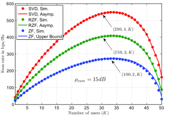
Figure 3: Sum rate performance for different systems with different precoders

where $\rho_{sum}$ denotes the total transmit SNR for all users. ‘Sim.’ and ‘Aysmp.’ are abbreviations for simulation and asymptotic results, respectively. As shown in Fig.3, our asymptotic sum rates and upper bound for $\mathcal{R}_{sum}^{ZF}$ are very tight even for small $M$ and $N$. And the sum rates of different precoders increase with $K$ firstly but decreases after a certain value of $K$ as analyzed above.

The optimal $K$ where the highest sum rate occurs, denoted by $K^{*}$, is

$$K^{*}=\arg\max_{K\in\mathcal{K}}\bar{\mathcal{R}}_{sum}$$ (15)

for a fixed $\rho$, where $\mathcal{K}$ is the set including all candidates of $K$, i.e., $\mathcal{K}\in\left\{1,\dots,\left\lfloor\beta\right\rfloor\right\}$. The exact $K^{*}$ involves solving the equations with the form of $x=\log_{2}\left(1+x\right)$, which can not be concluded into an explicit form. However, since $\bar{\mathcal{R}}_{sum}\left(\rho,K\right)$ is an unary offline function of $K$ for a given $\rho$, implementing $1-D$ searching over $\mathcal{K}$ is also a low-complexity solution.

The behavior of $K^{*}$ when $\rho$ increases is evaluated in Fig. 4.

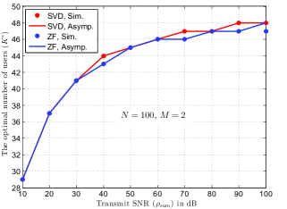
Figure 4: The optimal user number v.s. transmit SNR

Since RZF develops into ZF at high SNR regime, its behavior is omitted in the Fig. 4. It is observed that $K^{*}$ increases with $\rho$, which is corresponding to the previous analysis. The mismatches of ZF after $\rho_{sum}=90dB$ is likely caused by the usage of upper bound. It is obvious that serving users as large as possible guarantees the highest sum rate when the transmit power is unlimited. However, it also can be seen that $K^{*}$ being the maximum $K$ only happens at very high $\rho_{sum}$ (clearly should be greater than $100dB$), which indicates that making the system fully load ($K=\beta$) is not the best strategy when the transmit power is limited.

Specifically, $\Delta\bar{\mathcal{R}}_{sum}$, the increment of $\bar{\mathcal{R}}_{sum}$ brought by only adding one antenna at the BS compared to previous systems, is plotted in Fig. 5.

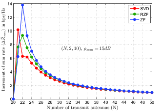
Figure 5: Increment of asymptotic sum rate brought by adding one antenna

For example, if the original system is a $\left(N,M,K\right)$ system, $\Delta\bar{\mathcal{R}}_{sum}$ donates the increment of $\bar{\mathcal{R}}_{sum}$ from $\left(N+1,M,K\right)$ to $\left(N,M,K\right)$, or from $\left(N+2,M,K\right)$ to $\left(N+1,M,K\right)$ and so on. In Fig. 5, the original system configuration is $\left(20,2,10\right)$, it is clear that $\bar{\mathcal{R}}_{sum}$ can be substantially improved by only adding a few antennas at the BS. That is because all the equivalent systems will have the same number of extra transmit antennas when more antennas are added at the BS. Hence, the increment of sum rate is multiplied by the number of users. While, $\Delta\bar{\mathcal{R}}_{sum}$ increases slowly when $N$ is getting large. Under such circumstance, it is the MU gain or DoFs that dominants the sum rate. Though the sum rate can always benefits from more antennas at the BS, it is worth noticing that $\Delta\bar{\mathcal{R}}_{sum}\rightarrow 0$ when $N\rightarrow\infty$, which can be proven by derivation of $\bar{\mathcal{R}}_{sum}$ with respect to $\beta$. Therefore, it is unnecessary to endow too many antennas at the BS by taking the expenses brought by them into consideration.

V Conclusion

In this paper, the tradeoff between MU gain and transmit diversity for MU-MIMO systems using BD technique is established. Specifically, a expression is derived to quantify how the two factors impact on the sum rate. Based on the tradeoff, the optimal number of users that maximizes the sum rate is obtained as well. The results in this paper have important significance for system configuration in practice. Note that the derivations is under the Rayleigh channels, they will be extended to other channel models in the future works.

References

• [1] J.Β Hoydis et. al., β€œMassive MIMO: How many antennas do we need?” in Proc. 49th Annu. Allerton Conf. on Communication, Control and Computing, Monticello, IL, 2011, pp. 545–550.
• [2] T.Β L.Β M. Hien QuocΒ Ngo, Erik G.Β Larsson, β€œEnergy and spectral efficiency of very large multiuser MIMO systems,” IEEE Trans. Commun., to be published.
• [3] F.Β Rusek, D.Β Persson, B.Β K. Lau, E.Β G. Larsson, T.Β L. Marzetta, O.Β Edfors, and F.Β Tufvesson, β€œScaling up MIMO: Opportunities and challenges with very large arrays,” IEEE Signal Processing Mag., vol.Β 30, no.Β 1, pp. 40–60, Jan. 2013.
• [4] B.Β Hochwald and S.Β Vishwannath, β€œSpace-time multiple access: Linear growth in the sum-rate,” in Proc. 40th Annu. Allerton Conf. on Communication, Control and Computing, Monticello, IL, 2002.
• [5] S.Β Wagner, R.Β Couillet, M.Β Debbah, and D.Β T.Β M. Slock, β€œLarge system analysis of linear precoding in correlated MISO broadcast channels under limited feedback,” IEEE Trans. Inf. Theory, vol.Β 58, no.Β 7, pp. 4509–4537, Jul. 2012.
• [6] L.Β Choi and R.Β D. Murch, β€œA transmit preprocessing technique for multiuser MIMO systems using a decomposition approach,” IEEE Trans. Wireless Commun., vol.Β 3, no.Β 1, pp. 20–24, Jan. 2004.
• [7] S.Β Shim, J.Β Kwak, R.Β Heath, and J.Β Andrews, β€œBlock diagonalization for multi-user MIMO with other-cell interference,” IEEE Trans. Wireless Commun., vol.Β 7, no.Β 7, pp. 2671–2681, Jul. 2008.
• [8] A.Β Tulino and A.Β Lozano, β€œMIMO capacity with channel state information at the transmitter,” in Proc. IEEE ISSTA, Boston, MA, 2004, pp. 22–26.
• [9] Z.Β D. Bai, β€œMethodologies in spectral analysis of large dimensional random matrices,” Statistica Sinica, vol.Β 9, pp. 611–661, 1999.
• [10] A.Β M. Tulino and S.Β VerdΓΊ, Random matrix theory and wireless communications.Β Β Β Boston, MA: Now Publishers Inc., 2004.
• [11] A.Β Goldsmith, Wireless Communications.Β Β Β Cambridge, UK: Cambridge University Press, 2005.