Mapping the differential reddening in globular clusters

Abstract

We build differential-reddening maps for 66 Galactic globular clusters (GCs) with archival HST WFC/ACS F606W and F814W photometry. Because of the different GC sizes (characterised by the half-light radius $R_{h}$) and distances to the Sun, the WFC/ACS field of view ($200\arcsec\times 200\arcsec$) coverage ($R_{obs}$) lies in the range $1\la R_{obs}/R_{h}\la 15$ for about $85\%$ of the sample, with about 10% covering only the inner ($R_{obs}\la R_{h}$) parts. We divide the WFC/ACS field of view across each cluster in a regular cell grid, and extract the stellar-density Hess diagram from each cell, shifting it in colour and magnitude along the reddening vector until matching the mean diagram. Thus, the maps correspond to the internal dispersion of the reddening around the mean. Depending on the number of available stars (i.e. probable members with adequate photometric errors), the angular resolution of the maps range from $\approx 7\arcsec\times 7\arcsec$ to $\approx 20\arcsec\times 20\arcsec$. We detect spatially-variable extinction in the 66 globular clusters studied, with mean values ranging from $\mbox{$\langle{\mbox{$\delta\mbox{$E(B-V)$}$}}\rangle$}\approx 0.018$ (NGC 6981) up to $\mbox{$\langle{\mbox{$\delta\mbox{$E(B-V)$}$}}\rangle$}\approx 0.16$ (Palomar 2). Differential-reddening correction decreases the observed foreground reddening and the apparent distance modulus but, since they are related to the same value of $E(B-V)$, the distance to the Sun is conserved. Fits to the mean-ridge lines of the highly-extincted and photometrically scattered globular cluster Palomar 2 show that age and metallicity also remain unchanged after the differential-reddening correction, but measurement uncertainties decrease because of the reduced scatter. The lack of systematic variations of $\langle{\mbox{$\delta\mbox{$E(B-V)$}$}}\rangle$ with both the foreground reddening and the sampled cluster area indicates that the main source of differential reddening is interstellar.

1 Introduction

Spatially-variable extinction, or differential reddening (hereafter DR), occurs in all directions throughout the Galaxy and is also present across the field of view of most globular clusters (GCs). By introducing non-systematic confusion in the actual colour and magnitude of member stars located in different parts of a GC, it leads to a broadening of evolutionary sequences in the colour-magnitude diagram (CMD). Thus, together with significant photometric scatter, unaccounted-for DR hampers the detection of multiple-population sequences and may difficult the precise determination of fundamental parameters, especially the age, metallicity and distance of GCs.

Over the years, several approaches have been used to map DR across the field of particular GCs, mostly focusing on rather restricted stellar evolutionary stages of the CMD. A rather comprehensive review of early works can be found in Alonso-García et al. (2011, 2012). More recently, Milone et al. (2012a) study the DR of 59 GCs observed with the Hubble Space Telescope (HST) WFC/ACS. Their method involves defining a fiducial line for the main-sequence (MS) and measuring the displacement (along the reddening vector) in apparent distance modulus and colour for all MS stars. This correction proved to be important for a better characterization of multiple sub-giant branch populations in NGC 362, NGC 5286, NGC 6656, NGC 6715, and NGC 7089 (Piotto et al. 2012). Alonso-García et al. (2011, 2012) search for DR in several GCs observed with the Magellan 6.5m telescope and HST. Their approach is similar to that of Milone et al. (2012a) but, instead of restricting to the MS, they build a mean ridge line (MRL) for most of the evolutionary stages expected of GC stars. Along similar lines, Massari et al. (2012) use HST WFC/ACS photometry to estimate the DR in the highly-extincted stellar system Terzan 5, which presents an average (mostly foreground) colour excess of $\mbox{$E(B-V)$}=2.38$. They build a regular grid of $25\times 25$ cells across the field of view of Terzan 5 and search for spatial variations, with respect to the bluest cell, in the mean colour and magnitude of MS stars extracted within each cell. The cell to cell differences in the mean (apparent distance modulus and colour) values are entirely attributed to internal reddening variations, which they find to reach a dispersion of $\mbox{$E(B-V)$}\sim 0.67$ around the mean.

In the present paper we use archival HST WFC/ACS data to estimate the differential reddening in a large sample of Galactic GCs. Our approach incorporates some of the features of the previous works, while including others that we propose to represent improvements. For instance, we use all the evolutionary sequences present in the CMD of a GC, take the photometric uncertainties explicitly into account, and exclude obvious non-member stars to build the Hess diagram. Thus, instead of defining a fiducial line, we use the actual stellar density distribution present in the Hess diagram of all stars as the template against which internal reddening variations are searched for. In short, we divide the on-the-sky projected stellar distribution in a spatial grid, extract the CMD of each cell, convert it into the Hess diagram, and find the reddening value that leads to the best match of this cell with the template Hess diagram. The final product is a DR map with a projected spatial resolution directly related to the number of stars available in the image. This, in turn, can be used to obtain the DR-corrected CMD.

This paper is organised as follows: in Sect. 2 we briefly discuss the data and the photometric cuts applied. In Sect. 3 we describe the approach adopted. In Sect. 4 we discuss the results for the GC sample. Concluding remarks are given in Sect. 5.

2 The GC sample

Most of the GCs focused here are part of the HST WFC/ACS sample obtained under program number GO 10775, with A. Sarajedini as PI, which guarantees some uniformity on data reduction and photometric quality. GO 10775 is a HST Treasury project in which 66 GCs were observed through the F606W and F814W filters. For symmetry reasons, we work only with GCs centred on the images. Also, for statistical reasons (Sect. 3), our approach requires a minimum of $\sim 3000$ stars (probable members with adequate colour uncertainty) available in the CMD. Both restrictions reduced the sample to 60 GCs. In addition, we include the 6 GCs (Pyxis, Ruprecht 106, IC 4499, NGC 6426, NGC 7006, and Palomar 15) observed with WFC/ACS under program GO 11586, with A. Dotter as PI. These 6 GCs satisfy our symmetry/number of stars conditions. Further details on the observations and data reduction are in Milone et al. (2012a) and Dotter, Sarajedini & Anderson (2011), respectively for both samples. The final sample contains 66 GCs.

The field of view of WFC/ACS is $\approx 200\arcsec\times 200\arcsec$, which implies that, depending on the GC distance and intrinsic size, different fractions of the angular distribution of cluster stars are covered by the observations. We characterize this effect by measuring the ratio between the maximum separation reached by WFC/ACS ($\approx 100\arcsec$) computed at the GC distance and its half-light radius (taken from the 2010 update of Harris 1996 - hereafter H10), $\mbox{$\mathcal{S}$}\equiv R_{obs}/R_{h}$. The results are given in Table 1. A first-order analysis of the structural parameters in H10 shows that the tidal and half-light radii relate linearly as $R_{t}\sim 10\,R_{h}$. Thus, in most cases we are sampling the very inner GC parts, since $\approx 10\%$ of our sample has $\mbox{$\mathcal{S}$}\leq 1$, such as in the case of NGC 6397 and NGC 6656; most of the sample, $\approx 85\%$, lies in the range spanned by $1\leq\mbox{$\mathcal{S}$}\leq 15$, with 4 GCs (NGC 4147, Palomar 15, Palomar 2, NGC 7006) reaching higher coverage levels.

Still regarding the photometric quality, Anderson et al. (2008) show that unmodelable PSF variations introduce a slight shift in the photometric zero point as a function of the star’s location in the field. The shifts cancel out when large areas are considered, but may be as large as $\pm 0.02$ mag in colour when comparing stars extracted from different, small areas across the field of GCs. In addition, they note that this residual variation is very hard to distinguish from actual spatially-variable reddening. We’ll return to this point in Sect. 4.

Galactic GCs suffer from varying fractions of field-star contamination (Milone et al. 2012a). Since comparison fields obtained with the same instrumentation are not available, we minimise non-member contamination in our analysis by applying colour-magnitude filters to exclude obvious field stars. These filters are designed to exclude stars with colour and/or magnitude clearly discordant from those expected of GC stellar evolutionary sequences. For high-quality photometry, these filters are more significant for fainter stars. We designed filters for each GC individually, respecting particularities associated with the CMD morphology (e.g. the presence of a blue horizontal branch or a red clump, blue stragglers, etc.) and photometric uncertainties. A typical example of such a filter is shown in Fig. 1 for NGC 1261.

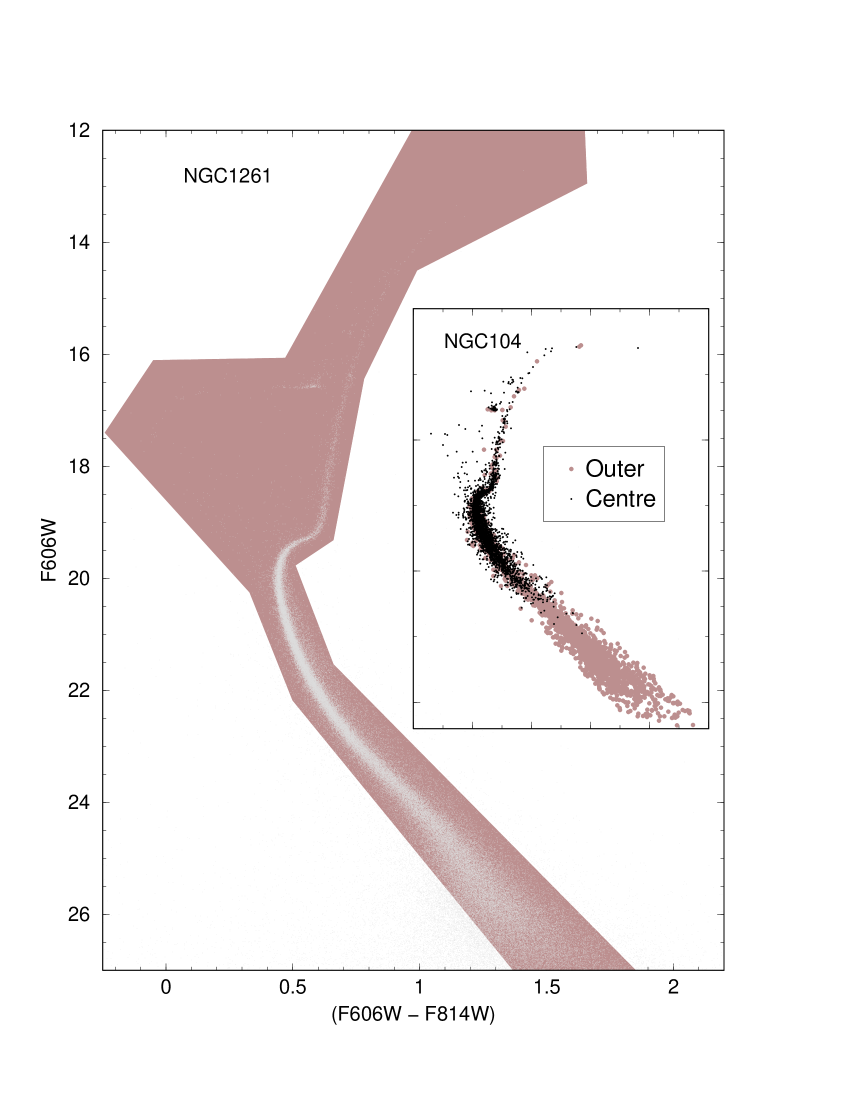
Figure 1: Example of a colour-magnitude filter (shaded polygon) used to minimize field contamination on NGC 1261. The inset shows morphological differences in CMDs extracted from the relatively crowded centre and an outer region of NGC 104.

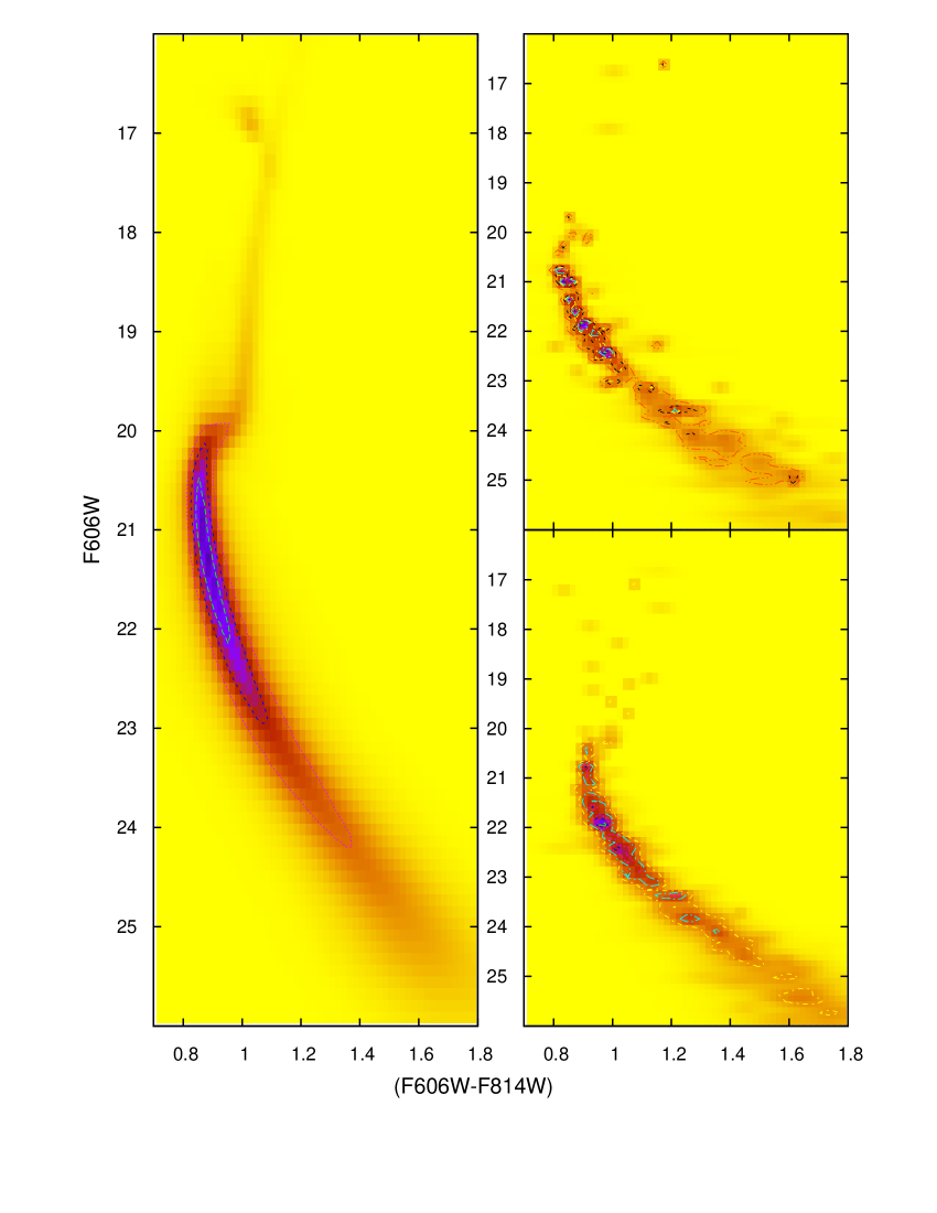
Figure 2: The bluest (top-right panel) and reddest (bottom-right) Hess diagrams of NGC 6388 are compared to the mean (observed) one (left). The difference in reddening between both amounts to $\mbox{$\delta\mbox{$E(B-V)$}$}=0.133$.

Despite the high quality of the sample, photometric uncertainties, which increase towards fainter magnitudes, may lead to a significant broadening of the lower main sequence. Thus, as an additional photometric quality control, we discard any star with colour uncertainty ($\sigma_{col}$) higher than a given threshold ($\sigma_{max}$). For statistical reasons, we work with $\sigma_{col}$ between 0.2 and 0.4 mag, lower for GCs with a high number of available stars ($\ga 2\times 10^{5}$) and increasing otherwise. Depending on the photometric quality and the amount of field-star contamination, the colour-magnitude filter combined to the $\sigma_{col}$ criterion exclude, on average, $\sim 15-40\%$ of the stars originally available in the CMDs. Parameters of the GC sample are given in Table 1, where the Galactic coordinates and the foreground reddening are taken from H10.

3 The adopted approach

The underlying concept is that, if DR is non negligible, CMDs extracted in different parts of a GC would be similar to each other but shifted along the reddening vector by an amount proportional to the relative extinction between the regions. In this sense, minimization of the differences by matching the CMDs can, in principle, be used to search for the extinction values affecting different places of a GC.

Obviously, differences between CMDs extracted from various parts of the same GC are expected to occur either by dynamical evolution (e.g. mass/luminosity segregation), by the presence of multiple populations (e.g. Milone et al. 2012b and references therein), or by observational limitations (e.g. crowding tends to produce a deficiency of faint stars in the central parts of a GC with respect to the outer parts). For instance, the latter effect is clearly illustrated by the CMDs of NGC 104 extracted at the relatively crowded centre and in a ring $\sim 100\arcsec$ away from it (inset of Fig. 1), a sparser region that allows detection of fainter stars. Then, a direct comparison between a central and an outer CMD might come up with differences that could be erroneously interpreted as DR. Thus, to minimize effects unrelated to DR, CMDs extracted in different parts of a GC are compared to the mean CMD. Specifically, the mean CMD contains all the WFC/ACS image stars that remain after we apply our photometric criteria (Sect. 2). Statistically, the mean CMD displays the spatially-averaged colour and magnitude properties of a GC, weighted according to the number of stars in each region. In this sense, variations detected among CMDs extracted in different parts of a GC should reflect the dispersion of reddening around the mean value. In addition, since the mean CMD contains the highest (with respect to the partial CMDs) number of stars, this procedure maximizes the statistical significance of the CMD comparison.

Figure 3: Convergence pattern ($R_{rms}$ as a function of $e(B-V)$) computed for the bluest (solid line) and reddest (dashed) cells of selected GCs.

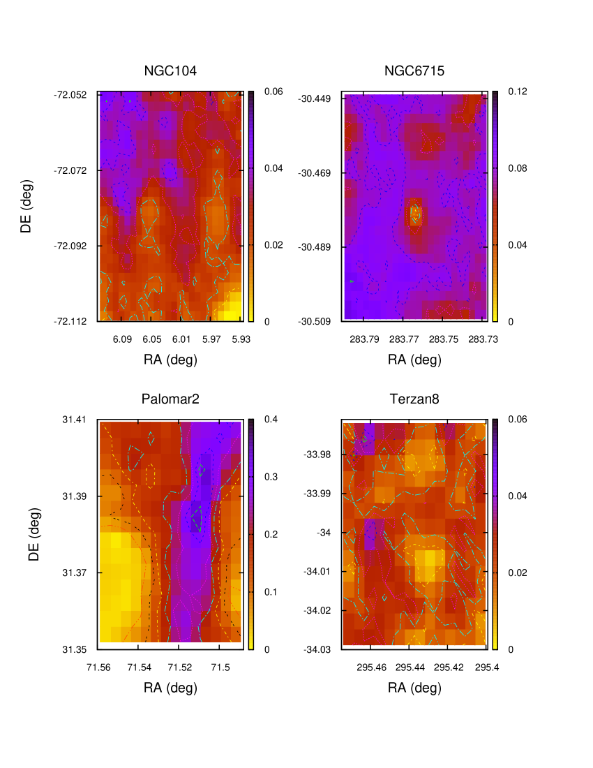
Figure 4: Differential-reddening maps of NGC 104, NGC 6715, Palomar 2 and Terzan 8. The range of values of $\delta\mbox{$E(B-V)$}$ is shown by the vertical bars.

However, the direct comparison between CMDs may also introduce some additional problems. Among these, we call attention to the discreteness associated with CMDs (especially those built with a small number of stars) and the remaining photometric uncertainties (see Sect. 2). To minimize these effects, we work with the (rather continuous) Hess diagram.

Photometric uncertainties - which are assumed to be Normally distributed - are taken into account when building the Hess diagrams. Formally, if the magnitude (or colour) of a given star is given by $\bar{x}\pm\sigma$, the probability of finding it at a specific value $x$ is given by $P(x)=\frac{1}{\sqrt{2\pi}\sigma}\,e^{{-\frac{1}{2}}\left(\frac{x-\bar{x}}{\sigma}\right)^{2}}$. Thus, for each star we compute the fraction of the magnitude and colour that occurs in a given bin of a Hess diagram, which corresponds to the difference of the error functions computed at the bin borders; by definition, the sum of the density over all Hess bins is the number of input stars. Since we are comparing cells with unequal numbers of stars, the corresponding Hess diagrams are normalized to unity, so that differences in number counts do not introduce biases into the analysis.

Then, the on-the-sky stellar distribution of the remaining stars ($N_{CMD}$) is divided in a grid of cells with a dimension that depends on the number of stars, and the CMD of each cell is extracted and converted into a Hess diagram. As an additional quality constraint, we only compute DR for cells having a number of stars higher than a minimum value $N_{min}$. After some tests, we settled for the range $50\leq N_{min}\leq 150$, higher for the GCs with more stars available. The spatial grid dimensions range from $30\times 30$ to $10\times 10$, with resolution increasing with the number of stars. Consequently, the angular resolution of the DR maps range from $\approx 7\arcsec\times 7\arcsec$ to $\approx 20\arcsec\times 20\arcsec$. Grid resolution, $N_{min}$, $\sigma_{max}$, and $N_{CMD}$, are listed in Table 1 for all GCs. Finally, we search for the optimum value of $\delta\mbox{$E(B-V)$}$ that leads to the best match between the Hess diagram of a cell and that of the whole distribution. The reddening vector has axes with amplitudes corresponding to the absorption relations $A_{F606W}=2.86\mbox{$\delta\mbox{$E(B-V)$}$}$ and $A_{F814W}=1.88\mbox{$\delta\mbox{$E(B-V)$}$}$, derived according to Cardelli, Clayton & Mathis (1989) for a G2V star.

Part of this process is illustrated in Fig. 2, in which the Hess diagrams of the bluest and reddest cells of NGC 6388 are compared to the overall/mean one. Except for the evolved sequences (and the relative stellar density), the bluest and reddest cell diagrams have similar morphologies, differing somewhat in magnitude and colour.

As discussed above, our approach assumes that DR plays the dominant role in producing variations such as those in Fig. 3 among CMDs extracted in different regions of the same GC. Consequently, this reduces the problem to searching for a single parameter, namely the internal colour excess $\delta\mbox{$E(B-V)$}$ difference between regions. We achieve this by minimising the root mean squared residuals ($R_{rms}$) between the mean ($\overline{H}$) Hess diagram and that extracted from a given cell ($H_{c}$), each composed of $n$ and $m$ colour and magnitude bins, where

$$\mbox{$R_{rms}$}=\sqrt{\frac{1}{N_{c}}\sum_{i,j=1}^{n,m}\frac{\left[\overline{H}(i,j)-H_{c}(i,j)\right]^{2}}{\left[\overline{H}(i,j)+H_{c}(i,j)\right]}}~{}~{}~{}.$$ (1)

The sum is restricted to non-empty Hess bins, and the normalisation by the total density in each bin gives a higher weight to the more populated bins. Finally, the squared sum is divided by the number of stars in the cell, which makes $R_{rms}$ dimensionless, and preserves the number statistics when comparing the convergence pattern for cells with unequal numbers of stars. All things considered, the relative weight that each evolutionary sequence has in the analysis is proportional to the respective Hess stellar density, roughly the number of stars it contains.

To minimise $R_{rms}$ we use the global optimisation method known as adaptive simulated annealing (ASA), because it is relatively time efficient, robust and capable of finding the optimum minimum (e.g. Goffe, Ferrier & Rogers 1994; Bonatto, Lima & Bica 2012; Bonatto & Bica 2012). Since the CMD cells may be somewhat bluer or redder than the mean one, the search starts with the parameter $e(B-V)$ being free to vary between $-0.5$ and $+0.5$. The initial trial point is randomly selected within this range and the starting value of $R_{rms}$ is computed. Then ASA takes a step by changing the initial parameter, and a new value of $R_{rms}$ is evaluated. Specifically, this implies that all stars in the cell have their colour and magnitude changed according to the new value of $e(B-V)$. By definition, any $R_{rms}$-decreasing (downhill) move is accepted, with the process repeating from this new point. Uphill moves may also be taken, with the decision made by the Metropolis (Metropolis et al. 1953) criterion, which enables ASA to escape from local minima. Variation steps become smaller as the minimisation is successful and ASA approaches the global minimum.

We illustrate the convergence pattern ($R_{rms}$ as a function of $e(B-V)$) for the bluest and reddest cells of some representative GCs in Fig. 3. Regardless of the number of available GC stars, low for NGC 6144 ($\sim 2\times 10^{4}$) and higher for Palomar 2 ($\sim 4.2\times 10^{4}$), NGC 1261 ($\sim 8.4\times 10^{4}$), and NGC 6388 ($\sim 2.7\times 10^{5}$), the $R_{rms}$ shape is similar, presenting a conspicuous and rather deep minimum, which is easily retrieved by our approach.

Table 1: General properties and derived parameters of the GC sample

GC	$\ell$	$b$	$\mathcal{S}$	$n_{RA}\times n_{DE}$	$N_{min}$	$\sigma_{max}$	$N_{CMD}$	$E(B-V)$	$\langle{\mbox{$\delta\mbox{$E(B-V)$}$}}\rangle$	$\mbox{$\delta\mbox{$E(B-V)$}$}_{max}$
	($\degr$)	($\degr$)		(cells)	(stars)	(mag)	($10^{4}$ stars)	(mag)	(mag)	(mag)
(1)	(2)	(3)	(4)	(5)	(6)	(7)	(8)	(9)	(10)	(11)
NGC 6441	$353.53$	$-5.01$	10	$30\times 30$	150	0.2	28.6	0.47	$0.069\pm 0.036$	0.175
NGC 6388	$345.56$	$-6.74$	9.0	$25\times 25$	150	0.2	27.0	0.37	$0.047\pm 0.019$	0.133
NGC 5139	$309.10$	$14.97$	0.5	$30\times 30$	150	0.2	26.9	0.12	$0.028\pm 0.009$	0.050
NGC 2808	$282.19$	$-11.25$	6.0	$30\times 30$	150	0.2	25.8	0.22	$0.028\pm 0.011$	0.068
NGC 6715	$5.61$	$-14.09$	15	$25\times 25$	150	0.2	23.4	0.15	$0.077\pm 0.010$	0.101
NGC 7089	$53.37$	$-35.77$	5.4	$25\times 25$	150	0.2	20.9	0.06	$0.032\pm 0.009$	0.055
NGC 7078	$65.01$	$-27.31$	5.2	$25\times 25$	150	0.2	19.9	0.10	$0.032\pm 0.014$	0.065
NGC 5024	$332.96$	$79.76$	6.8	$25\times 25$	150	0.2	19.9	0.02	$0.030\pm 0.009$	0.068
NGC 5286	$311.61$	$10.57$	8.0	$25\times 25$	125	0.3	17.6	0.24	$0.061\pm 0.017$	0.112
NGC 5272	$42.22$	$78.71$	2.2	$25\times 25$	150	0.3	15.0	0.01	$0.031\pm 0.009$	0.063
NGC 104	$305.89$	$-44.89$	0.7	$25\times 25$	125	0.3	14.8	0.04	$0.028\pm 0.009$	0.051
NGC 6205	$59.01$	$40.91$	2.1	$25\times 25$	125	0.3	13.9	0.02	$0.026\pm 0.009$	0.054
NGC 5986	$337.02$	$13.27$	5.3	$25\times 25$	150	0.3	13.6	0.28	$0.048\pm 0.022$	0.111
NGC 6341	$68.34$	$34.86$	4.1	$25\times 25$	125	0.3	12.3	0.02	$0.030\pm 0.010$	0.064
NGC 1851	$244.51$	$-35.03$	11	$25\times 25$	125	0.3	12.0	0.02	$0.025\pm 0.010$	0.054
NGC 6093	$352.67$	$19.46$	8.2	$23\times 23$	100	0.3	11.3	0.18	$0.039\pm 0.015$	0.078
NGC 362	$301.53$	$-46.25$	5.2	$23\times 23$	100	0.3	10.5	0.05	$0.032\pm 0.009$	0.056
NGC 5904	$3.86$	$46.80$	2.1	$23\times 23$	100	0.3	10.3	0.03	$0.033\pm 0.009$	0.068
NGC 6541	$349.29$	$-11.19$	3.5	$23\times 23$	100	0.3	10.1	0.14	$0.033\pm 0.017$	0.092
NGC 1261	$270.54$	$-52.12$	11	$23\times 23$	100	0.3	8.4	0.01	$0.024\pm 0.008$	0.049
NGC 5927	$326.60$	$4.86$	3.5	$23\times 23$	100	0.3	8.4	0.45	$0.059\pm 0.031$	0.169
NGC 6656	$9.89$	$-7.55$	0.5	$23\times 23$	100	0.3	8.3	0.34	$0.047\pm 0.018$	0.100
NGC 6304	$355.83$	$5.38$	2.1	$20\times 20$	100	0.2	7.3	0.54	$0.047\pm 0.020$	0.109
NGC 6779	$62.66$	$8.34$	4.3	$23\times 23$	80	0.3	6.9	0.26	$0.052\pm 0.018$	0.093
NGC 7099	$27.18$	$-46.84$	3.9	$20\times 20$	80	0.3	6.0	0.03	$0.030\pm 0.010$	0.064
NGC 6934	$52.10$	$-18.89$	11	$20\times 20$	80	0.3	5.9	0.10	$0.031\pm 0.012$	0.069
NGC 4833	$303.60$	$-8.02$	1.4	$20\times 20$	80	0.3	5.6	0.32	$0.042\pm 0.015$	0.093
NGC 7006	$63.77$	$-19.41$	46	$15\times 15$	100	0.3	5.5	0.05	$0.030\pm 0.010$	0.055
NGC 6101	$317.74$	$-15.82$	7.3	$20\times 20$	80	0.3	5.4	0.05	$0.026\pm 0.009$	0.054
NGC 6723	$0.07$	$-17.30$	2.8	$18\times 18$	80	0.3	5.4	0.05	$0.027\pm 0.009$	0.051
NGC 6254	$15.14$	$23.08$	1.1	$18\times 18$	80	0.3	5.2	0.28	$0.060\pm 0.023$	0.117
NGC 6637	$1.72$	$-10.27$	5.2	$18\times 18$	80	0.3	5.1	0.18	$0.031\pm 0.007$	0.058
NGC 4590	$299.63$	$36.05$	3.4	$18\times 18$	80	0.3	5.0	0.05	$0.046\pm 0.017$	0.089
NGC 6584	$342.14$	$-16.41$	9.0	$18\times 18$	80	0.3	4.9	0.10	$0.029\pm 0.009$	0.055
IC 4499	$307.35$	$-20.47$	5.5	$18\times 18$	100	0.3	4.7	0.23	$0.031\pm 0.012$	0.064
NGC 6752	$336.49$	$-25.63$	1.0	$18\times 18$	80	0.3	4.4	0.04	$0.030\pm 0.012$	0.064
NGC 6426	$28.09$	$16.23$	11	$15\times 15$	100	0.3	4.3	0.36	$0.047\pm 0.022$	0.097
NGC 6624	$2.79$	$-7.91$	4.8	$18\times 18$	80	0.3	4.3	0.28	$0.047\pm 0.019$	0.114
Palomar 2	$170.53$	$-9.07$	25	$15\times 15$	80	0.3	4.2	1.24	$0.161\pm 0.090$	0.375

• Col. 1: GC identification; Cols. 2 and 3: Galactic coordinates; Col. 4: Fraction of the half-maximum radius covered by WFC/ACS; Col. 5: RA and DEC grid; Col. 6: Minimum number of stars for a cell to be used in DR computation; Col. 7: Maximum allowed colour uncertainty; Col. 8: Number of stars remaining after applying the colour-magnitude filter and with $\sigma_{col}\leq\sigma_{max}$; Col. 9: Foreground reddening (H10); Col. 10: Mean differential colour excess (values lower than 0.04 may be related to zero-point variations); Col. 11: Maximum value reached by the differential colour excess.

Table 2: continued

GC	$\ell$	$b$	$\mathcal{S}$	$n_{RA}\times n_{DE}$	$N_{min}$	$\sigma_{max}$	$N_{CMD}$	$E(B-V)$	$\langle{\mbox{$\delta\mbox{$E(B-V)$}$}}\rangle$	$\mbox{$\delta\mbox{$E(B-V)$}$}_{max}$
	($\degr$)	($\degr$)		(cells)	(stars)	(mag)	($10^{4}$ stars)	(mag)	(mag)	(mag)
(1)	(2)	(3)	(4)	(5)	(6)	(7)	(8)	(9)	(10)	(11)
NGC 6809	$8.79$	$-23.27$	1.0	$20\times 20$	80	0.4	3.8	0.08	$0.027\pm 0.010$	0.050
NGC 6681	$2.85$	$-12.51$	6.3	$15\times 15$	80	0.4	3.7	0.07	$0.024\pm 0.007$	0.041
NGC 6981	$35.16$	$-32.68$	9.0	$16\times 16$	80	0.4	3.2	0.05	$0.018\pm 0.008$	0.038
NGC 6218	$15.72$	$26.31$	1.3	$18\times 18$	80	0.3	2.8	0.19	$0.027\pm 0.008$	0.056
NGC 3201	$277.23$	$8.64$	0.8	$18\times 18$	80	0.4	2.7	0.24	$0.057\pm 0.019$	0.118
Lynga 7	$328.77$	$-2.80$	3.3	$15\times 15$	80	0.4	2.6	0.73	$0.073\pm 0.037$	0.191
NGC 6362	$325.55$	$-17.57$	1.8	$18\times 18$	80	0.4	2.5	0.09	$0.025\pm 0.008$	0.046
NGC 5466	$42.15$	$73.59$	3.5	$18\times 18$	80	0.4	2.4	0.01	$0.024\pm 0.009$	0.048
NGC 288	$152.30$	$-89.38$	2.0	$15\times 15$	60	0.4	2.1	0.03	$0.047\pm 0.018$	0.091
Terzan 8	$5.76$	$-24.56$	13	$15\times 15$	80	0.4	2.0	0.12	$0.022\pm 0.010$	0.055
NGC 6144	$351.93$	$15.70$	2.7	$15\times 15$	60	0.4	1.9	0.36	$0.038\pm 0.016$	0.079
NGC 2298	$245.63$	$-16.00$	5.5	$15\times 15$	60	0.4	1.8	0.14	$0.062\pm 0.024$	0.126
NGC 6652	$1.53$	$-11.38$	10	$15\times 15$	60	0.4	1.8	0.09	$0.025\pm 0.008$	0.047
NGC 6171	$3.37$	$23.01$	1.8	$13\times 13$	50	0.4	1.8	0.33	$0.061\pm 0.025$	0.112
NGC 6352	$341.42$	$-7.17$	1.4	$15\times 15$	60	0.4	1.7	0.22	$0.042\pm 0.018$	0.092
NGC 5053	$335.70$	$78.95$	3.3	$15\times 15$	60	0.4	1.7	0.01	$0.029\pm 0.011$	0.058
NGC 4147	$252.85$	$77.19$	20	$13\times 13$	50	0.4	1.7	0.02	$0.019\pm 0.009$	0.045
Rup 106	$300.88$	$11.67$	10	$15\times 15$	70	0.5	1.7	0.20	$0.026\pm 0.010$	0.051
NGC 6397	$338.17$	$-11.96$	0.4	$13\times 13$	60	0.4	1.3	0.18	$0.019\pm 0.009$	0.051
Arp 2	$8.55$	$-20.79$	8.0	$15\times 15$	60	0.4	1.0	0.10	$0.026\pm 0.010$	0.059
NGC 6838	$56.75$	$-4.56$	1.2	$11\times 11$	50	0.4	0.9	0.25	$0.035\pm 0.015$	0.074
Terzan 7	$3.39$	$-20.07$	14	$11\times 11$	50	0.4	0.8	0.07	$0.033\pm 0.011$	0.055
NGC 6717	$12.88$	$-10.90$	5.2	$11\times 11$	50	0.4	0.8	0.22	$0.025\pm 0.010$	0.057
Palomar 15	$18.88$	$24.30$	20	$11\times 11$	50	0.5	0.7	0.40	$0.033\pm 0.014$	0.088
Pyxis	$261.32$	$7.00$	—	$11\times 11$	50	0.5	0.7	0.21	$0.038\pm 0.012$	0.070
NGC 6366	$18.41$	$16.04$	0.6	$13\times 13$	50	0.4	0.6	0.71	$0.055\pm 0.018$	0.112
NGC 6535	$27.18$	$10.44$	4.0	$10\times 10$	50	0.4	0.3	0.34	$0.020\pm 0.011$	0.044

4 Results

The first step is to compute $e(B-V)$, the internal difference in $E(B-V)$ of all cells with respect to the mean Hess diagram. Once the bluest cell is identified, we compute its difference in $e(B-V)$ with respect to the other cells, thus giving rise to the actual distribution of DR values $\delta\mbox{$E(B-V)$}$ in a given GC. Cells having a number of stars lower than $N_{min}$ (usually those lying at the image borders) are attributed a $\delta\mbox{$E(B-V)$}$ corresponding to the average among the nearest neighbour cells. Finally, the colour and magnitude of all stars in a cell are corrected for the corresponding $\delta\mbox{$E(B-V)$}$, a process that is repeated for all cells in the grid. What emerges from this procedure is the corresponding DR map, such as those illustrated in Fig. 4, and the DR-corrected CMDs (e.g. Fig. 5).

Figure 5: CMDs of selected GCs before (left panels) and after (right) differential-reddening correction. For visualization purposes, arbitrary shifts have been applied to the colour axis.

Our approach computes colour shifts among stars extracted from different regions across the GCs. Thus, before proceeding into the analysis, we have to consider the potential effects of unaccounted-for zero-point variations across the respective fields. As discussed in Anderson et al. (2008), stars extracted from wide-apart regions may present a difference in colour (related to zero-point variation) of $\Delta(F_{606W}-F_{814W})\leq 0.04$, which our approach would take as a difference in reddening of $\mbox{$\delta\mbox{$E(B-V)$}$}\leq 0.04$. Correction for this residual zero-point variation would require having access to a detailed map of the shifts for all GCs in Table 1. Since this information is not available, in what follows we either call attention to or exclude from the analysis the GCs in which colour shifts due to zero-point variation may dominate over differential reddening.

The DR maps shown in Fig. 4 are typical among our GC sample. They show that extinction may be patchy (as in the centre of NGC 6715) and scattered (as across Terzan 8), rather uniform (as in Palomar 2, where it is apparently distributed as a thin dust cloud lying along the north-south direction), or somewhat defining a gradient (like in NGC 104). However, most of the cells in NGC 104 have $\mbox{$\delta\mbox{$E(B-V)$}$}\leq 0.04$ (Table 1 and Fig. 6), which suggests that most of the colour pattern across its field is extrinsic, probably related to the zero-point variation.

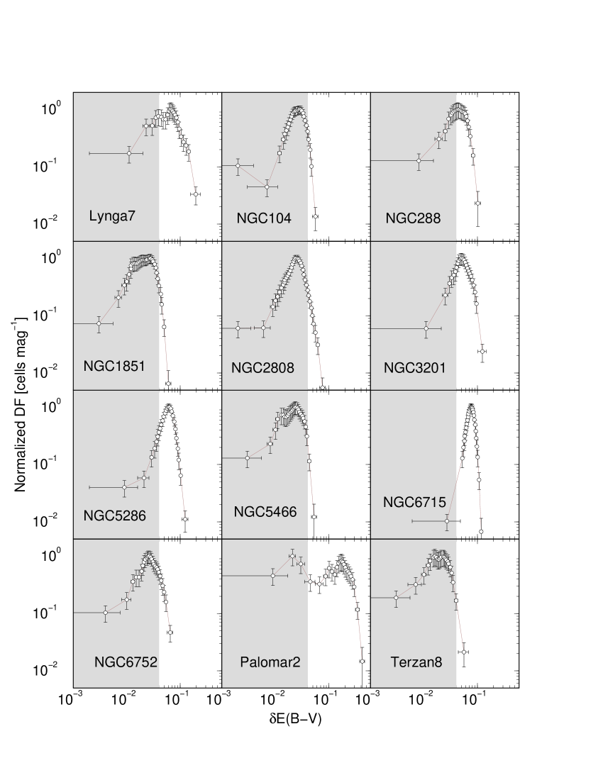
Figure 6: Distribution function of $\delta\mbox{$E(B-V)$}$ for a representative GC sub-sample. For comparison purposes, the DFs are normalized to the peak. Values within the shaded area may be affected by residual zero-point variations.

Turns out that our approach is capable of detecting some measurable amount of DR in the 66 GCs dealt with in this paper. To summarize this point, we show in Fig. 6 the distribution function (DF) of the $\delta\mbox{$E(B-V)$}$ measured over all cells of selected GCs, from which the mean and maximum DR values, $\langle{\mbox{$\delta\mbox{$E(B-V)$}$}}\rangle$ and $\mbox{$\delta\mbox{$E(B-V)$}$}_{max}$, can be measured. Some GCs, like NGC 104, NGC 2808, NGC 5286, and NGC 6715, have roughly log-normal DFs, while in others like Palomar 2, the DFs are flat and broad. The majority ($67\%$) of the GCs have the mean DR characterized by $\mbox{$\langle{\mbox{$\delta\mbox{$E(B-V)$}$}}\rangle$}\la 0.04$ (a range of values that may be mostly related to zero-point variations), with the highest value $\mbox{$\langle{\mbox{$\delta\mbox{$E(B-V)$}$}}\rangle$}=0.161$ occurring in Palomar 2. Regarding the maximum DR value, 67% of the GCs have $\mbox{$\mbox{$\delta\mbox{$E(B-V)$}$}_{max}$}\la 0.09$, with the highest $\mbox{$\mbox{$\delta\mbox{$E(B-V)$}$}_{max}$}=0.375$ again in Palomar 2. For a more objective assessment of the range of $\delta\mbox{$E(B-V)$}$ occurring in the GCs, we give in Table 1 the average and maximum values of $\delta\mbox{$E(B-V)$}$ found for each GC.

By construction, when our approach corrects a CMD cell by the corresponding DR value, it shifts both the colour and magnitude of all stars in the cell towards smaller values of apparent distance modulus and colour excess. Thus, the correction brings together the cell’s photometric scatter that, after applying to all cells, makes the blue and red CMD ridges somewhat bluer. We note that this same effect shows up in the CMDs of Terzan 5, for which a different approach was applied by Massari et al. (2012) to correct for DR (see their Fig. 4). In addition, since the reddening vector for F606W and F814W is roughly directed along the MS, the colour and distance modulus shift should be more conspicuous in the evolved sequences, as shown in Fig. 5 for selected GCs.

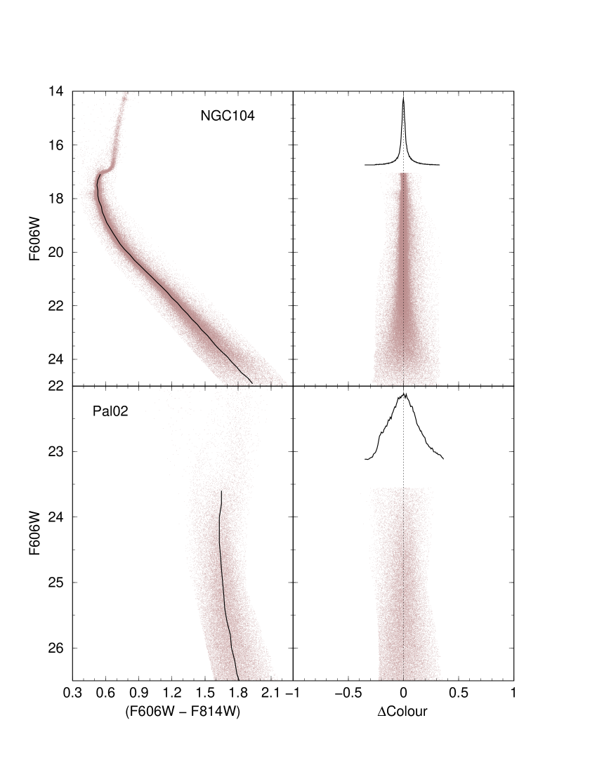
Figure 7: The fiducial line (solid curve, left panels) is used to rectify the main sequence (right panels), from which the residual colour distribution is computed (inset in right panels).

For a more objective assessment of the changes introduced by our DR correction into the CMDs, we examine the colour spread along the main sequence. The first step involves rectifying the main sequence, which is achieved by subtracting - for each star - the colour corresponding to the fiducial line, which basically traces the highest-density track of the CMD (or Hess diagram). In the present cases, we divide the main-sequence in bins 0.1 or 0.2 mag wide (depending on the number of stars in each bin) and build the distribution function for the colour of all stars within each bin. Then, we fit a Gaussian to the distribution function, from which we take the colour corresponding to the highest stellar density - which represents the fiducial colour for the mid-point of the bin. After subtracting the fiducial line, we build the residual colour distribution function (i.e. the number-density of stars within a given colour bin) for the full magnitude range of the main sequence. This process is illustrated in Fig. 7 for NGC 104 and Palomar 2, previous to DR correction. The markedly different residual colour distributions (quite narrow for NGC 104 and broad for Palomar 2) reflect the very different DR properties of both GCs (Table 1 and Fig. 6). Figure 8 shows the residual colour distributions (restricted to the main sequence) before and after DR correction for selected GCs. The narrowing effect on the main sequence is conspicuous, especially for the highest differentially-reddened GC of our sample, Palomar 2.

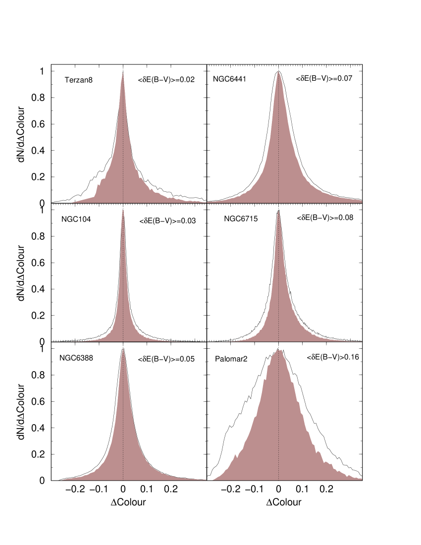
Figure 8: Residual colour distribution function of the main sequence of selected GCs before (solid curve) and after (shaded curve) differential-reddening correction.

We further illustrate our approach in Fig. 9 with NGC 2298 ($\mbox{$E(B-V)$}=0.14$, $\mbox{$\langle{\mbox{$\delta\mbox{$E(B-V)$}$}}\rangle$}=0.062$, $\mbox{$\mbox{$\delta\mbox{$E(B-V)$}$}_{max}$}=0.126$), displaying the results in a similar fashion as in Milone et al. (2012a), which also serves to compare the different approaches more objectively. As expected, the DR correction decreases the colour spread over most of the rectified main sequence. To better quantify the colour spread, we build the colour distribution function for each interval $\Delta F606W=1$ mag, within the range $19-24$ (similar to that used by Milone et al. 2012a). Finally, we fit a Gaussian to these functions, from which we measure the dispersion ($\sigma_{c}$) around the mean colour spread. Both before and after DR correction, $\sigma_{c}$ increases towards fainter magnitudes; obviously, $\sigma_{c}$ values measured after DR correction are smaller than the respective ones before correction. Although following a similar pattern, our $\sigma_{c}$ values are a little lower than those found by Milone et al. (2012a). This difference is possibly related to the fact the first step into the analysis involves excluding probable field stars (with colours excessively red or blue with respect to the expected GC evolutionary sequence) by using the colour-magnitude filter (Sect. 2). As an additional comparison, both the North-South gradient pattern indicated by our approach for the differential reddening in NGC 6366 (Fig. 2 in Campos et al. 2013) and the relative reddening values (Table 1) are consistent with those found by Alonso et al. (1997), $\Delta\mbox{$E(B-V)$}\approx 0.03$ between both hemispheres.

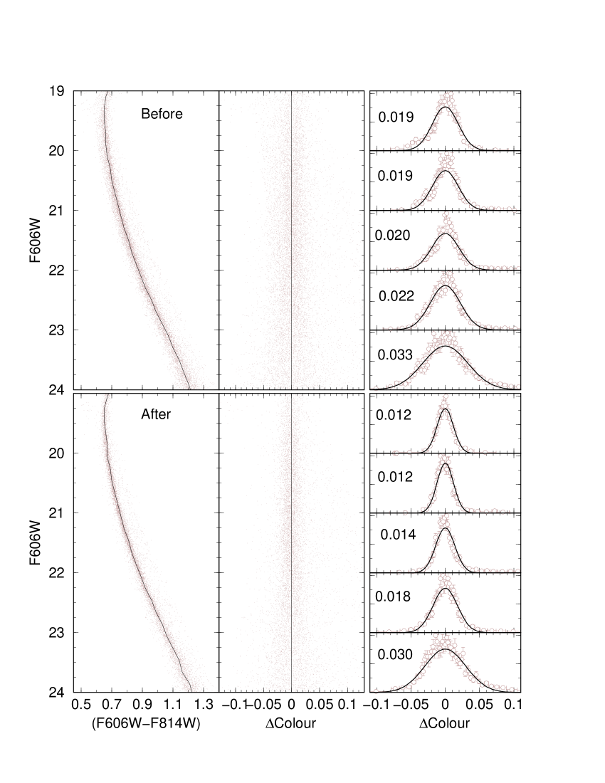
Figure 9: The major part of the main sequence of NGC 2298 shown before (top panels) and after (bottom) DR correction. Subtraction of the fiducial line (left panels) allows visualization of the colour spread along the rectified main sequence (middle). The intrinsic colour dispersion is measured in intervals of 1 mag by means of Gaussian fit to the distribution function (right); the measured dispersion ($\sigma_{c}$) is given in each panel (in all cases the uncertainty in $\sigma_{c}$ is $\leq 0.001$).

An observational consequence of correcting a CMD for DR is a slight decrease in the apparent distance modulus and colour excess by amounts related to $E(B-V)$ according to the adopted reddening vector. Consequently, the GC distance to the Sun should remain unchanged, since the distance decrease implied by the smaller apparent distance modulus is exactly compensated by the increase associated with the lower foreground colour-excess.

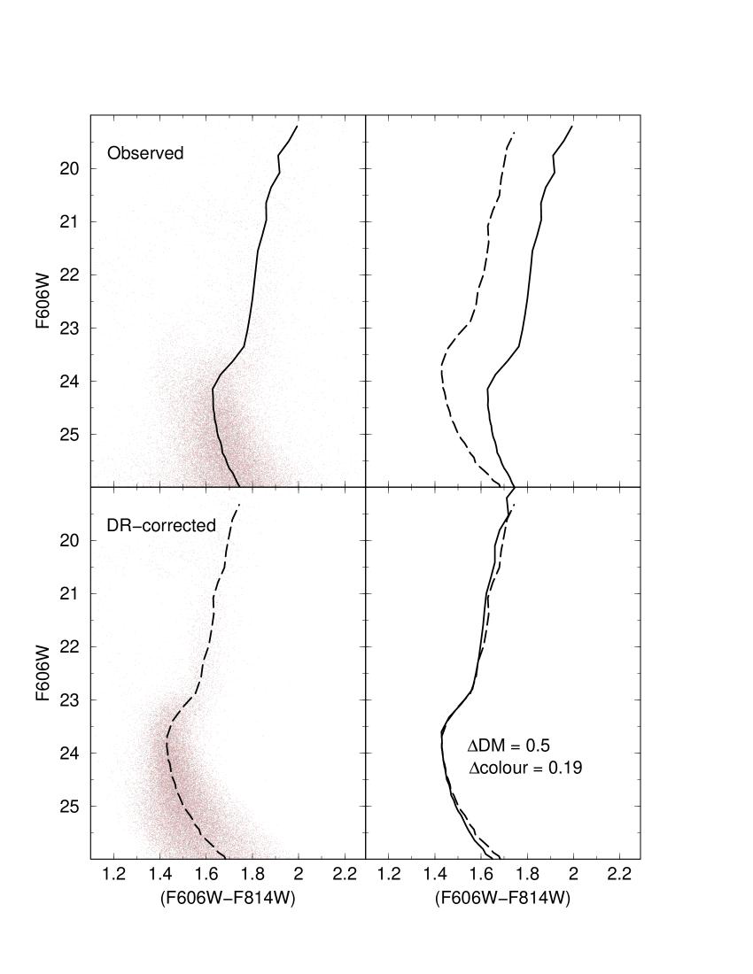
Figure 10: Differences in colour-excess and apparent distance modulus between the mean-ridge lines of the observed and DR-corrected CMDs of Palomar 2 (left-panels) are significant (top-right). They are minimized by decreasing the observed distance modulus by 0.5 mag and the foreground reddening by 0.19 mag (bottom-right).

Figure 10 illustrates the above issue with Palomar 2, the worst-case scenario in terms of mean, maximum (Table 1) and distribution of DR values (Fig. 6), as well as photometric scatter. We first build the mean-ridge line (MRL) for the MS, sub-giant and red-giant branches both for the observed (top-left panel) and DR-corrected (bottom-left) CMDs. The differences in apparent distance modulus and foreground colour excess become clear when both MRLs are placed on the same panel (top-right). A near-match of both MRLs occurs when the apparent distance modulus and the colour excess of the observed CMD are shifted by $\Delta(m-M)_{F606W}=-0.5$ and $\Delta(F606W-F814W)=-0.19$, respectively. For these filters, the ratio between the DR-corrected ($d_{c}$) and observed ($d_{o}$) distances can be expressed as $\log(d_{c}/d_{o})=\left(\Delta(m-M)_{F606W}-2.92\times\Delta(F606W-F814W)\right)/5$. For the MRLs of Palomar 2, the shifts produce a small increase ($\approx 3\%$) in the distance, probably lower than the observational uncertainties. Thus, given the lower DR values and photometric scatter of the remaining GCs of our sample, the corresponding changes in distance should be lower than that of Palomar 2.

Since the mean CMD morphology is essentially conserved by the DR correction, age and metallicity determinations based on MRLs are expected to come up with unchanged results as well, but their measured uncertainties should decrease, as the overall CMD scatter is reduced.

By definition, foreground reddening is the amount of extinction that affects uniformly all stars in a CMD. In this context, it is obvious that not all of the extinction needs to be actually located outside the cluster. For instance, suppose a GC affected by an internal DR distribution in which the minimum value is higher than zero and with no intervening extinction. Consequently, the minimum DR value would be mistaken as foreground. In this sense, our analysis above shows that part of the assumed foreground reddening may in fact be internal. In the case of Palomar 2, the DR correction makes the overall CMD bluer by about $\Delta\mbox{$E(B-V)$}=-0.2$, thus implying a lower foreground reddening than that given in H10 (and reproduced in Table 1).

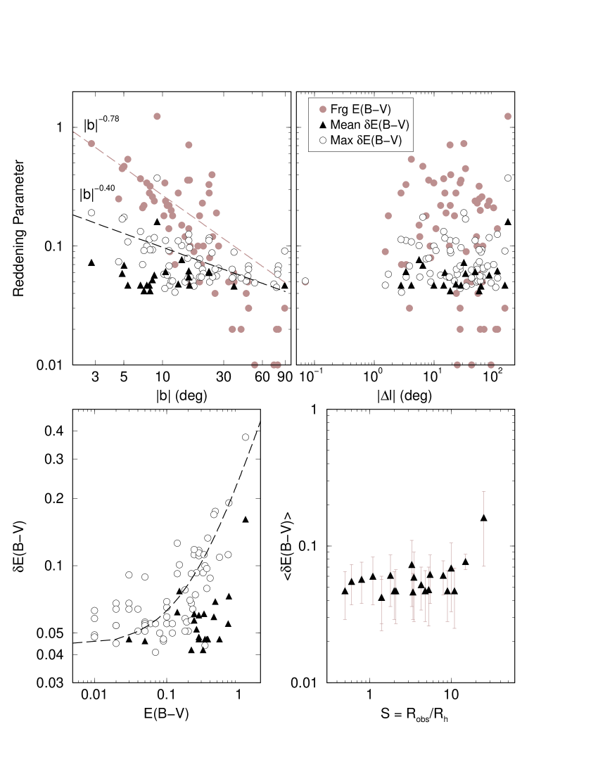
Figure 11: Dependence of foreground, mean and maximum differential-reddening values on the angular distance to the Galactic plane (top-left panel), and to the centre (top-right). The dependence on $|b|$ is characterized by power-law fits with the indicated slopes (dashed lines). $\mbox{$\delta\mbox{$E(B-V)$}$}_{max}$ correlates with $E(B-V)$ as a straight line (bottom-left). There is no correlation between $\langle{\mbox{$\delta\mbox{$E(B-V)$}$}}\rangle$ and the GC area covered by WFC/ACS (bottom-right).

Finally, in Fig. 11 we study dependences and correlations among the derived parameters. In this analysis we exclude the GCs having the maximum and mean DR lower than 0.04 mag; the final sub-samples contain 65 GCs with $\mbox{$\mbox{$\delta\mbox{$E(B-V)$}$}_{max}$}>0.04$ and only 22 with $\mbox{$\langle{\mbox{$\delta\mbox{$E(B-V)$}$}}\rangle$}>0.04$. Both the foreground and maximum reddening parameters appear to anti-correlate with the distance to the Galactic plane ($|b|$) at different degrees (top-left panel); the mean-DR, on the other hand, presents an essentially flat distribution of values. As expected, the foreground absorption $E(B-V)$ clearly increases towards the Galactic plane according to $\mbox{$E(B-V)$}=(1.59\pm 0.44)\times|b|^{-(0.78\pm 0.13)}$, with the mild correlation coefficient $CC=0.63$. A similar, but shallower dependence occurs for the maximum DR, $\mbox{$\mbox{$\delta\mbox{$E(B-V)$}$}_{max}$}=(0.24\pm 0.05)\times|b|^{-(0.40\pm 0.08)}$, with $CC=0.48$.

Both $\mbox{$\delta\mbox{$E(B-V)$}$}_{max}$ and $\langle{\mbox{$\delta\mbox{$E(B-V)$}$}}\rangle$ are similarly uncorrelated with the angular distance to the Galactic centre ($|\Delta\ell|$); the same occurs with the foreground $E(B-V)$, but with the scatter having larger amplitude (top-right panel). Regarding the dependence on the foreground $E(B-V)$, the maximum DR values appear to increase with $E(B-V)$ especially for $\mbox{$E(B-V)$}\ga 0.2$ (bottom-left panel). Indeed, the best representation for $\mbox{$\delta\mbox{$E(B-V)$}$}_{max}$ is a straight line, $\mbox{$\mbox{$\delta\mbox{$E(B-V)$}$}_{max}$}=(0.043\pm 0.004)+(0.20\pm 0.01)\times\mbox{$E(B-V)$}$, with the strong correlation coefficient $CC=0.85$. The restriction to $\mbox{$\langle{\mbox{$\delta\mbox{$E(B-V)$}$}}\rangle$}\geq 0.04$ precludes a similar fit to $\langle{\mbox{$\delta\mbox{$E(B-V)$}$}}\rangle$, but it also appears to increase for $\mbox{$E(B-V)$}\ga 0.2$. This suggests that interstellar (external) reddening is the dominant source of DR.

The issue concerning the internal/external to the clusters nature of the differential-reddening source can be investigated from another perspective. Although the fraction of the cluster area covered by WFC/ACS $\mbox{$\mathcal{S}$}\equiv R_{obs}/R_{h}$ varies significantly among our sample (Table 1), its effect on the mean DR values is essentially negligible (Fig. 11, bottom-right). A reasonable assumption is that, if the source of DR is essentially internal to the clusters, with the dust distribution following the cluster stellar structure, differences in $\delta\mbox{$E(B-V)$}$ - and thus the mean DR - should increase with $\mathcal{S}$. In this context, the lack of a systematic variation of $\langle{\mbox{$\delta\mbox{$E(B-V)$}$}}\rangle$ with $\mathcal{S}$ indicates that most of the DR source is external to the clusters, which is consistent with the conclusion of the previous paragraph.

5 Summary and conclusions

In this work we derive the differential-reddening maps of 66 Galactic globular clusters from archival HST WFC/ACS data uniformly observed (and reduced) with the F606W and F814W filters. The angular resolution of the maps are in the range $\approx 7\arcsec\times 7\arcsec$ to $\approx 20\arcsec\times 20\arcsec$. According to current census (Ortolani et al. 2012, and references therein), our sample comprises about 40% of the Milky Way’s globular cluster population, which implies that the results can be taken as statistically significant.

We start by dividing the WFC/ACS field of view across a given GC in a regular grid with a cell resolution that varies with the number of available stars. Next, we select a sub sample of stars containing probable members having low to moderate colour uncertainty. Then, the stellar-density Hess diagrams built from CMDs extracted in different cells of the grid are matched to the mean one (containing all the probable-member stars available in the WFC/ACS image) by shifting the apparent distance modulus and colour excess along the reddening vector by amounts related to the reddening value $e(B-V)$ according to the absorption relations in Cardelli, Clayton & Mathis (1989). This is equivalent to computing the reddening dispersion around the mean, since a differentially-reddened cluster should contain cells bluer and redder than the mean. Finally, we compute the difference in $e(B-V)$ between all cells and the bluest one, thus yielding the cell to cell distribution of $\delta\mbox{$E(B-V)$}$, from which we compute the mean and maximum values occurring in a given GC, $\langle{\mbox{$\delta\mbox{$E(B-V)$}$}}\rangle$ and $\mbox{$\delta\mbox{$E(B-V)$}$}_{max}$, respectively. This process also gives rise to the DR maps and the DR-corrected CMDs.

We find spatially-variable extinction in the 66 GCs studied in this paper, with mean values (with respect to the cell to cell distribution) ranging from $\mbox{$\langle{\mbox{$\delta\mbox{$E(B-V)$}$}}\rangle$}\approx 0.018$ (NGC 6981) up to $\mbox{$\langle{\mbox{$\delta\mbox{$E(B-V)$}$}}\rangle$}\approx 0.16$ (Palomar 2). As a caveat, we note that values of $\mbox{$\delta\mbox{$E(B-V)$}$}\la 0.04$ may be related to uncorrected zero-point variations in the original photometry. By comparing dependences of the DR-related parameters with the distance to the Galactic plane, foreground reddening, and cluster area sampled by WFC/ACS, we find that the main source of differential reddening is interstellar (external to the GCs).

Regarding the CMD analyses based on mean-ridge lines (and theoretical isochrones), the DR correction decreases both the apparent distance modulus and foreground reddening values, but does not change the observed distance to the Sun, age and metallicity. Besides, the measured uncertainties in these fundamental parameters are expected to decrease, since the overall CMD scatter is reduced. Anyone interested in having access to the code and/or DR maps built in this paper - or having the data of specific GCs analysed by us - should contact C. Bonatto.

References

- Alonso et al. (1997) Alonso A., Salaris M., Martínez-Roger C., Straniero O. & Arribas S. 1997, A&A, 323, 374
- Alonso-García et al. (2012) Alonso-García J., Mateo M., Sen B., Banerjee M. & von Braun K. 2011, AJ, 141, 146
- Alonso-García et al. (2011) Alonso-García J., Mateo M., Sen B., Banerjee M., Catelan M., Minniti D. & von Braun K. 2012, AJ, 143, 70
- Anderson et al. (2008) Anderson J., Sarajedini A., Bedin L.R., King I.R., Piotto G., Reid I.N., Siegel M., Majewski S.R. et al. 2008, AJ, 135, 2055
- Bonatto & Bica (2012) Bonatto C. & Bica E. 2012, MNRAS, 423, 1390
- Bonatto, Lima & Bica (2012) Bonatto C., Lima E.F. & Bica E. 2012, A&A, 540A, 137
- Campos et al. (2013) Campos F., Kepler S.O., Bonatto C. & Ducati J.R. 2013, MNRAS, in press
- Cardelli, Clayton & Mathis (1989) Cardelli J.A., Clayton G.C. & Mathis J.S. 1989, ApJ, 345, 245
- Dotter, Sarajedini & Anderson (2011) Dotter A., Sarajedini A. & Anderson J. 2011, ApJ, 738, 74
- Goffe, Ferrier & Rogers (1994) Goffe W.L., Ferrier G.D. & Rogers J. 1994, Journal of Econometrics, 60, 65
- Harris (1996) Harris W.E. 1996, AJ, 112, 1487 (2010 edition at arXiv:1012.3224)
- Hess (1924) Hess R. 1924, in Die Verteilungsfunktion der absol. Helligkeiten etc. Probleme der Astronomie. Festschrift fur Hugo v. Seeliger. (Berlin:Springer), 265
- Massari et al. (2012) Massari D., Mucciarelli A., Dalessandro E., Ferraro F.R.. Origlia L., Lanzoni B., Beccari G., Rich R.M. et al. 2012, ApJL, 755, 32
- Metropolis et al. (1953) Metropolis N., Rosenbluth A., Rosenbluth M., Teller A. & Teller, E. 1953, Journal of Chemical Physics, 21, 1087
- Milone et al. (2012a) Milone A.P., Piotto G., Bedin L.R., Aparicio A., Anderson J., Sarajedini A., Marino A.F., Moretti A. et al. 2012a, A&A, 540A, 16
- Milone et al. (2012b) Milone A.P., Marino A.F., Cassisi S., Piotto G., Bedin L.R., Anderson J., Allard F., Aparicio A. et al. 2012b, ApJ, 754L, 34
- Ortolani et al. (2012) Ortolani S., Bonatto C., Bica E., Barbuy B. & Saito R.K. 2012, AJ, AJ, 144, 147
- Piotto et al. (2012) Piotto G., Milone A.P., Anderson J., Bedin L.R., Bellini A., Cassisi S., Marino A.F., Aparicio A. et al. 2012, ApJ, 760, 39