A reduced new modified Weibull distribution

Abstract

In this paper, we propose a reduced version of the new modified Weibull (NMW) distribution due to Almalki and Yuan [2] in order to avoid some estimation problems. The number of parameters in the NMW distribution is five. The number of parameters in the reduced version is three. We study mathematical properties as well as maximum likelihood estimation of the reduced version. Four real data sets (two of them complete and the other two censored) are used to compare the flexibility of the reduced version versus the NMW distribution. It is shown that the reduced version has the same desirable properties of the NMW distribution in spite of having two less parameters. The NMW distribution did not provide a significantly better fit than the reduced version for any of the four data sets.

Keywords. Hazard rate function; Maximum likelihood estimation; Weibull distribution.

1 Introduction

In reliability engineering and lifetime analysis many applications require a bathtub shaped hazard rate function. The traditional Weibull distribution [27], which includes the exponential and Rayleigh distributions as particular cases, is one of the important lifetime distributions. Unfortunately, however, it does not exhibit a bathtub shape for its hazard rate function. Many researchers have proposed modifications and generalizations of the Weibull distribution to accommodate bathtub shaped hazard rates. Extensive reviews of these modifications have been presented by many authors, see, for example, Rajarshi and Rajarshi [20], Murthy et al. [15], Pham and Lai [18] and Lai et al. [11].

Although some flexible distributions among these modifications have only two or three parameters (for example, the flexible Weibull extension [4], the modified Weibull (MW) distribution [12] and the modified Weibull extension [29]), most modifications of the Weibull distribution have four or five parameters. By combining two Weibull distributions, with one having an increasing hazard rate function and the other decreasing one, Xie and Lai [28] introduced a four-parameter distribution called the additive Weibull (AddW) distribution. Sarhan and Apaloo [22] proposed the exponentiated modified Weibull extension which exhibits a bathtub shaped hazard rate. Sarhan et al. [21] proposed the exponentiated generalized linear exponential distribution which generalizes a large set of distributions including the exponentiated Weibull distribution. Famoye et al. [7] proposed the beta-Weibull (BWD) distribution with unimodal, increasing, decreasing or bathtub shaped hazard rate functions. Another four-parameter distribution, called the generalized modified Weibull (GMW) distribution, was proposed by Carrasco et al. [5]. The hazard rate function of this distribution can be increasing, decreasing, bathtub shaped or unimodal. Cordeiro et al. [6] introduced the Kumaraswamy Weibull (KumW) distribution and studied its mathematical properties extensively. It has four parameters, three of which are shape parameters, making it so flexible. Its hazard function can be constant, increasing, decreasing, bathtub shaped or unimodal. A five-parameter distribution was introduced as a modification of the Weibull distribution by Phani [19]. This distribution generalizes the four-parameter Weibull distribution proposed by Kies [8]. Another five-parameter distribution, the beta modified Weibull (BMW) distribution, was introduced by Silva et al. [25]. It allows for different hazard rate shapes: increasing, decreasing, bathtub shaped and unimodal. It was shown to fit bathtub shaped data sets very well. Recently, a new five-parameter distribution called the beta generalized Weibull distribution was proposed by Singla et al. [26]. The hazard rate function of this distribution can be increasing, decreasing, bathtub shaped or unimodal. It contains as sub-models some well known lifetime distributions.

Almalki and Yuan [2] introduced a new modified Weibull (NMW) distribution. It generalizes several commonly used distributions in reliability and lifetime data analysis, including the MW distribution, the AddW distribution, the modified Weibull distribution of Sarhan and Zaindin (SZMW) [23], the Weibull distribution, the exponential distribution, the Rayleigh distribution, the extreme-value distribution and the linear failure rate (LFR) [3] distribution. The cumulative distribution function (CDF) of the NMW distribution is

$$F(x)=1-e^{-\alpha x^{\theta}-\beta x^{\gamma}e^{\lambda x}}$$

for $x>0$, $\gamma>0$, $\theta>0$, $\alpha>0$, $\beta>0$ and $\lambda>0$, where $\gamma$, $\theta$ are shape parameters, $\alpha$, $\beta$ are scale parameters and $\lambda$ is an acceleration parameter. Almalki and Yuan [2] derived mathematical properties of this distribution as well as estimated its parameters by the method of maximum likelihood with application to real data sets.

The hazard rate function of the NMW distribution can be increasing, decreasing or bathtub shaped. It has been shown to be the best lifetime distribution to date in terms of fitting some popular and widely used real data sets like Aarset data [1] and voltage data [13].

Although distributions with four or more parameters are flexible and exhibit bathtub shaped hazard rates, they are also complex [16] and cause estimation problems as a consequence of the number of parameters, especially when the sample size is not large. The main purpose of this work is to reduce the number of parameters of the NMW distribution so as to address these problems while maintaining the same flexibility to fit data so well. This can be achieved by choosing the two shape parameters $\gamma=\theta=\frac{1}{2}$ as we now show.

There are various tools to assess the flexibility of a given univariate distribution. One commonly used tool is the kurtosis-skewness plot. Values of (skewness, kurtosis) plotted on the $(x,y)$ plane for all possible values of the parameters of the distribution give what is referred to as the kurtosis-skewness plot. The area or the range covered by the kurtosis-skewness plot is a measure of flexibility of the distribution.

The kurtosis-skewness plot for the NMW distribution is drawn on the left hand side of Figure . The values of (skewness, kurtosis) were computed over $\theta=0.1,0.2,\ldots,5$, $\gamma=0.1,0.2,\ldots,5$, $\theta=\gamma\neq\frac{1}{2}$, $\alpha=0.1,0.2,\ldots,2$, $\beta=0.1,0.2,\ldots,2$ and $\lambda=0.1,0.2,\ldots,2$. The kurtosis-skewness plot for the reduced distribution is drawn on the right hand side of Figure . The values of (skewness, kurtosis) were computed over $\alpha=0.1,0.2,\ldots,2$, $\beta=0.1,0.2,\ldots,2$ and $\lambda=0.1,0.2,\ldots,2$.

We can see that the particular case $\theta=\gamma=\frac{1}{2}$ is a flexible member of the NMW distribution. The range of kurtosis values is widest for the case $\theta=\gamma=\frac{1}{2}$. The range of skewness values is also widest for the case $\theta=\gamma=\frac{1}{2}$, but some negative skewness values are not accommodated by this case.

The rest of this paper is organized as follows. The reduced distribution is introduced in Section 2. Section 3 considers the hazard rate function of the reduced distribution. The moments, the moment generating function and the distribution of order statistics are derived as particular cases of the NMW distribution in Section 4. Section 5 discusses maximum likelihood estimation of the unknown parameters using complete and censoring data. Four real data sets, uncensored and censored, are analyzed in Section 6. Finally, Section 7 concludes the paper.

2 The reduced distribution

Setting $\gamma=\theta=\frac{1}{2}$ in the CDF of the NMW distribution, we obtain the CDF of the reduced new modified Weibull (RNMW) distribution as

$$F(x)=1-e^{-\alpha\sqrt{x}-\beta\sqrt{x}e^{\lambda x}}$$

for $x>0$, $\alpha>0$, $\beta>0$ and $\lambda>0$, where $\alpha$, $\beta$ are scale parameters and $\lambda$ is an acceleration parameter. This reduced version of the NMW distribution has a bathtub shaped hazard rate function, as will be shown later.

The corresponding probability density function (PDF) is

$$f(x)=\frac{1}{2\sqrt{x}}\left[\alpha+\beta(1+2\lambda x)e^{\lambda x}\right]e^{-\alpha\sqrt{x}-\beta\sqrt{x}e^{\lambda x}}$$

for $x>0$. The PDF of the RNMW distribution can be decreasing or decreasing then increasing-decreasing as shown in Figure 1. It is clear that the reduced distribution is nearly as flexible as the NMW distribution.

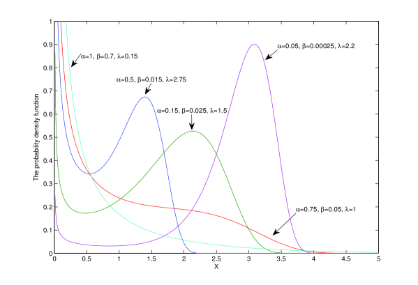
Figure 1: PDFs of the RNMW distribution.

3 The hazard rate function

The hazard rate function of the RNMW distribution is

$$h(x)=\frac{1}{2\sqrt{x}}\left[\alpha+\beta(1+2\lambda x)e^{\lambda x}\right]$$ (1)

for $x>0$. To derive the shape of $h(x)$, we obtain the first derivative of $\log\left\{{h(x)}\right\}$:

$$\frac{d}{dx}\log\left\{{h(x)}\right\}=-\frac{1}{2x}+\frac{\beta\lambda(2\lambda x+3)e^{\lambda x}}{\alpha+\beta(2\lambda x+1)e^{\lambda x}}.$$ (2)

Setting this to zero, we have

$$-\frac{1}{2x}+\frac{\beta\lambda(2\lambda x+3)e^{\lambda x}}{\alpha+\beta(2\lambda x+1)e^{\lambda x}}=0.$$ (3)

Let $x_{0}$ denote the root of (3). From (2), $\frac{d}{dx}\log\left\{{h(x)}\right\}<0$ for $x\in(0,x_{0})$, $\frac{d}{dx}\log\left\{{h(x_{0})}\right\}=0$, and $\frac{d}{dx}\log\left\{{h(x)}\right\}>0$ for $x>x_{0}$. So, $h(x)$ initially decreases before increasing. Hence, we have a bathtub shape. Let $x_{0}$ denote the solution of (3); that is, the solution of

$$\left(4\beta\lambda x^{2}+4\beta\lambda x-\beta\right)e^{\lambda x}=\alpha.$$ (4)

The left hand side of (4) is $e^{\lambda x}$ multiplied by the quadratic function $(4\beta\lambda x^{2}+4\beta\lambda x-\beta)$. The value $x_{0}$ is unique and positive as shown in Figure 2.

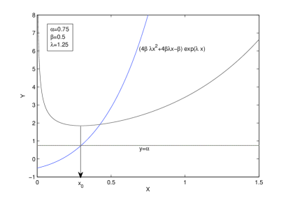
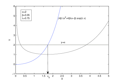
(a)	(b)

Figure 2: The root of $\frac{d}{dx}\log\left\{{h(x_{0})}\right\}=0$.

Plots of the hazard rate function of the RNMW distribution are shown in Figure 3 (a). Many different applications in reliability and lifetime analysis require bathtub shaped hazard rate functions with a long useful life period and the middle period of the bathtub shape having a relatively constant hazard rate (for example, electric machine life cycles and electronic devices [10]). The NMW distribution has this property, and so does the RNMW distribution, as Figure 3(b) shows.

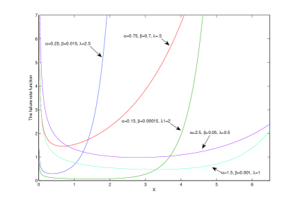
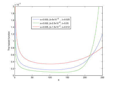
(a)	(b)

Figure 3: Hazard rate function of the RNMW distribution.

4 The moments, the moment generating function and order statistics

Let $X$ denote a random variable having the RNMW distribution. The $r$th moment of $X$ can be derived from Section 3.2 in Almalki and Yuan [2] as

$$\mu_{r}^{\prime}=2r\sum_{n,m=0}^{\infty}\frac{(-\beta)^{n}(n\lambda)^{m}}{n!m!}\frac{\Gamma\left(n+2(m+r)\right)}{\alpha^{n+2(m+r)}}$$ (5)

for $r=1,2,\ldots$. The moment generating function of $X$ is

$$M_{X}(t)=1+2\sum_{n,m,k=0}^{\infty}\frac{(-\beta)^{n}(n\lambda)^{m}t^{k+1}}{i!j!k!}\left[\frac{\Gamma\left(n+2(m+k)+2\right)}{\alpha^{n+2(m+k)+2}}\right],$$ (6)

see Appendix A for a proof. Using (6), the first four moments of $X$ are

$$M_{X}^{\prime}(0)=\mu_{1}^{\prime}=2\sum_{n,m=0}^{\infty}\frac{(-\beta)^{n}(n\lambda)^{m}}{i!j!k!}\left[\frac{\Gamma\left(n+2m+2\right)}{\alpha^{n+2m+2}}\right],$$

$$M_{X}^{\prime\prime}(0)=\mu_{2}^{\prime\prime}=4\sum_{n,m=0}^{\infty}\frac{(-\beta)^{n}(n\lambda)^{m}}{i!j!k!}\left[\frac{\Gamma\left(n+2m+4\right)}{\alpha^{n+2m+4}}\right],$$

$$M_{X}^{(3)}(0)=\mu_{3}^{(3)}=6\sum_{n,m=0}^{\infty}\frac{(-\beta)^{n}(n\lambda)^{m}}{i!j!k!}\left[\frac{\Gamma\left(n+2m+6\right)}{\alpha^{n+2m+6}}\right],$$

$$M_{X}^{(4)}(0)=\mu_{2}^{(4)}=8\sum_{n,m=0}^{\infty}\frac{(-\beta)^{n}(n\lambda)^{m}}{i!j!k!}\left[\frac{\Gamma\left(n+2m+8\right)}{\alpha^{n+2m+8}}\right].$$

These expressions are consistent with the formula for moments in (5).

Let $X_{1},\ldots,X_{n}$ denote a random sample drawn from the RNMW distribution with parameters $\alpha$, $\beta$ and $\lambda$. The PDF of the $r$th order statistic say $X_{(r)}$ can be derived as a particular case from Section 3.3 of [2]:

$${f}_{r:n}\left(x\right)=n\binom{n-1}{r-1}\sum\limits_{{\ell=0}}^{{r-1}}\binom{r-1}{\ell}\frac{(-1)^{\ell}}{(n+\ell+1-r)}f\left(x;\alpha_{\ell},\beta_{\ell},\lambda\right),$$

where $f(x;\alpha_{\ell},\beta_{\ell},\lambda)$ is the RNMW PDF with parameters $\alpha_{\ell}=(n+\ell+1-r)\alpha$, $\beta_{\ell}=(n+\ell+1-r)\beta$ and $\lambda$. The $k$th non-central moment of the $r$th order statistic is then

$${\mu}_{k}^{{}^{\prime}(r:n)}={2nk}\binom{n-1}{r-1}\sum_{i,j=0}^{\infty}\sum\limits_{{\ell=0}}^{{r-1}}\binom{r-1}{\ell}\frac{(-1)^{\ell+1}\beta^{i}(i\lambda)^{j}\Gamma\left(i+2(j+k)\right)}{\alpha^{i-1}\left[\alpha(n+\ell+1-r)\right]^{{2(j+k)}+1}}.$$

5 Parameter estimation

In this section, point and interval estimators of the unknown parameters of the RNMW distribution are derived using the maximum likelihood method. We consider both complete data and censored data.

5.1 Complete data

The PDF of the RNMW distribution can be rewritten as

$$f(x)=h\left(x;\underline{\vartheta}\right)e^{-\alpha\sqrt{x}-\beta\sqrt{x}e^{\lambda x}}$$

for $x>0$, where $h\left(x;\underline{\vartheta}\right)$ is the hazard rate function in (1) and $\underline{\vartheta}=(\alpha,\beta,\lambda)$ is a vector of parameters.

Let $x_{1},\ldots,x_{n}$ denote a random sample of complete data from the RNMW distribution. Then, the log-likelihood function is

$$\ell\left(\underline{\vartheta}\right)=\sum\limits_{i=1}^{n}\left[\log\left(h\left(x_{i};\underline{\vartheta}\right)\right)-\alpha\sqrt{x_{i}}-\beta\sqrt{x_{i}}e^{\lambda x_{i}}\right].$$

The likelihood equations are obtained by setting the first partial derivatives of $\ell$ with respect to $\alpha,\beta$ and $\lambda$ to zero; that is,

$$\sum\limits_{i=1}^{n}\frac{1}{h\left(x_{i};\alpha,\beta,\lambda\right)\left(2\sqrt{x_{i}}\right)}-\sum\limits_{i=1}^{n}{\sqrt{x_{i}}}=0,$$ (7)

$$\sum\limits_{i=1}^{n}\frac{\left(0.5+\lambda x_{i}\right)e^{\lambda x_{i}}}{h\left(x_{i};\alpha,\beta,\lambda\right)\sqrt{x_{i}}}-\sum\limits_{i=1}^{n}e^{\lambda x_{i}}\sqrt{x_{i}}=0,$$ (8)

$$\sum\limits_{i=1}^{n}\frac{\sqrt{x_{i}}\left(\frac{3}{2}+\lambda x_{i}\right)e^{\lambda x_{i}}}{h\left(x_{i};\alpha,\beta,\lambda\right)}-\sum\limits_{i=1}^{n}e^{\lambda x_{i}}\sqrt{x_{i}^{3}}=0.$$ (9)

5.2 Censored data

Here, we consider maximum likelihood estimation for censored data without replacement. Let $X_{i}$ and $C_{i}$ denote the lifetime and the censoring time for tested individual $i$, $i=1,\ldots,n$. Suppose $X_{i}$ and $C_{i}$ are independent random variables. The failure times are $x_{i}=\min(X_{i},C_{i})$, $i=1,\ldots,n$. Then, the log-likelihood function is

$$\ell\left(\underline{\vartheta}\right)=\sum\limits_{i=1}^{d}\log\left[h\left(x_{i};\underline{\vartheta}\right)-\alpha\sqrt{x_{i}}-\beta\sqrt{x_{i}}e^{\lambda x_{i}}\right]-\sum\limits_{i\in C}\left[\alpha\sqrt{x_{i}}+\beta\sqrt{x_{i}}e^{\lambda x_{i}}\right],$$

where $d$ is the number of failures and $C$ indexes the censored observations.

Setting the first partial derivatives of $\ell\left(\underline{\vartheta}\right)$ with respect to $\alpha$, $\beta$ and $\lambda$ to zero, the likelihood equations are obtained as

$$\sum\limits_{i=1}^{d}\left\{\frac{1}{h\left(x_{i};\alpha,\beta,\lambda\right)\left(2\sqrt{x_{i}}\right)}-\sqrt{x_{i}}\right\}-\sum\limits_{i\in C}\sqrt{x_{i}}=0,$$ (10)

$$\sum\limits_{i=1}^{d}\left\{\frac{\left(0.5+\lambda x_{i}\right)e^{\lambda x_{i}}}{h\left(x_{i};\alpha,\beta,\lambda\right)\sqrt{x_{i}}}-e^{\lambda x_{i}}\sqrt{x_{i}}\right\}-\sum\limits_{i\in C}\sqrt{x_{i}}e^{\lambda x_{i}}=0,$$ (11)

$$\sum\limits_{i=1}^{d}\left\{\frac{\sqrt{x_{i}}\left(\frac{3}{2}+\lambda x_{i}\right)e^{\lambda x_{i}}}{h\left(x_{i};\alpha,\beta,\lambda\right)}-e^{\lambda x_{i}}\sqrt{x_{i}^{3}}\right\}-\sum\limits_{i\in C}e^{\lambda x_{i}}\sqrt{x_{i}^{3}}=0.$$ (12)

By solving the systems of nonlinear likelihood equations, (7,8,9) and (10,11,12), numerically for $\alpha$, $\beta$ and $\lambda$, we can obtain maximum likelihood estimates for complete and censored data.

According to Miller [14], the MLEs ($\widehat{\alpha},\widehat{\beta},\widehat{\lambda}$) of ($\alpha,\beta,\lambda$) have an approximate multivariate normal distribution with mean ($\alpha$, $\beta$, $\lambda$) and variance-covariance matrix $\widehat{I^{-1}}$; that is,

$$\left(\widehat{\alpha},\widehat{\beta},\widehat{\lambda}\right)\sim N_{3}\left((\alpha,\beta,\lambda),\widehat{I^{-1}}\right),$$

where

$$I=-\left[\begin{array}[]{lll}\ell_{\alpha\alpha}&\ell_{\alpha\beta}&\ell_{\alpha\lambda}\\ &\ell_{\beta\beta}&\ell_{\beta\lambda}\\ &&\ell_{\lambda\lambda}\end{array}\right].$$

The second order partial derivatives of $\ell\left(\underline{\vartheta}\right)$ are given in Appendices B and C.

6 Applications

This section provides four applications, two of them are for complete (uncensored) data sets and the others are for censored data sets, to show how the RNMW distribution can be applied in practice. Almalki and Yuan [2] have shown that the NMW distribution fits data sets better than existing modifications of the Weibull distribution like the BMW distribution, the AddW distribution, the MW distribution and the SZMW distribution. So, we shall compare the fits of the RNMW and NMW distributions to see if the former can perform as well as the NMW distribution. The Kolmogorov-Smirnov (K-S) statistic (the distance between the empirical CDFs and the fitted CDFs), the Akaike information criterion (AIC), the Bayesian information criterion (BIC) and the consistent Akaike information criterion (CAIC) are used to compare the candidate distributions. The log-likelihood ratio test is used to compare the NMW and RNMW distributions by testing the hypotheses: $H_{0}:\theta=\gamma=\frac{1}{2}$ versus $H_{1}:H_{0}$ is false. The likelihood ratio test statistic for testing $H_{0}$ against $H_{1}$ is $\omega=2(\mathcal{L}_{NMW}-\mathcal{L}_{RNMW})$, which follows a $\chi^{2}$ distribution with two degrees of freedom under $H_{0}$.

6.1 Complete data

In this section, we show how the RNMW distribution can be applied in practice for two complete (uncensored) real data sets.

6.1.1 Aarset data

The Aarset data [1] consisting of lifetimes of fifty devices is widely used in lifetime analysis. The data set exhibits a bathtub shaped hazard rate. Both the NMW and RNMW distributions were fitted to this data set. Table 1 gives the MLEs of the parameters, corresponding standard errors, AIC, BIC, and CAIC. Table 2 provides the K-S test statistics. Figures 4a and 4b show the histogram of the data, PDFs of the fitted NMW and RNMW distributions, the empirical survival function, and the survival functions of the fitted NMW and RNMW distributions.

It is clear that both the NMW and RNMW distributions provide adequate fits. Both have very small K-S values (0.088 and 0.092, respectively). The NMW distribution has the larger log-likelihood of -212.9. However, the RNMW distribution has the smaller values for AIC, BIC and CAIC. The likelihood ratio test statistic for testing $H_{0}:\theta=\gamma=\frac{1}{2}$ versus $H_{1}:H_{0}$ is false is $\omega=1.436$ and the corresponding $p$-value is 0.488, so there is no evidence to reject $H_{0}$. Hence, the NMW distribution does not improve significantly on the fit of the RNMW distribution.

The plots of the empirical TTT-transform, TTT-transforms of the fitted NMW and RNMW distributions, the nonparametric hazard rate function, and the hazard rate functions of the fitted NMW and RNMW distributions are shown in Figures 4c and 4d. It is clear that the RNMW distribution provides as good a fit as the NMW distribution.

Table 1: MLEs of parameters, standard errors, AIC, BIC and CAIC for Aarset data.

Model	$\widehat{\alpha}$	$\widehat{\beta}$	$\widehat{\gamma}$	$\widehat{\theta}$	$\widehat{\lambda}$	AIC	BIC	CAIC
NMW	$0.071$	$7.015\times 10^{-8}$	$0.016$	$0.595$	$0.197$	$435.8$	$445.4$	$437.2$
	(0.031)	($1.501\times 10^{-7}$)	(3.602)	(0.128)	(0.184)
RNMW	$0.102$	$3.644\times 10^{-8}$	$\frac{1}{2}$	$\frac{1}{2}$	$0.180$	$433.1$	$439.0$	$433.8$
	(0.019)	($6.089\times 10^{-8}$)	$-$	$-$	(0.020)

Table 2: K-S statistics for models fitted to Aarset data.

Model								K-S
NMW								0.088
RNMW								0.092

The variance-covariance matrix for the fitted RNMW distribution is

$$I^{-1}=\left[\begin{array}[]{lll}5.203\times 10^{-4}&-3.697\times 10^{-9}&1.214\times 10^{-3}\\ -3.697\times 10^{-9}&9.078\times 10^{-14}&-2.994\times 10^{-8}\\ 1.214\times 10^{-3}&-2.994\times 10^{-8}&9.882\times 10^{-3}\end{array}\right].$$

So, approximate $95$ percent confidence intervals for the parameters $\alpha$, $\beta$ and $\lambda$ are $\left[0.064,0.14\right]$, $\left[0,1.558\times 10^{-7}\right]$ and $\left[0.219\times 10^{-5},0.142\right]$, respectively.

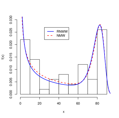
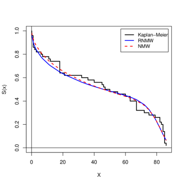
(a)	(b)
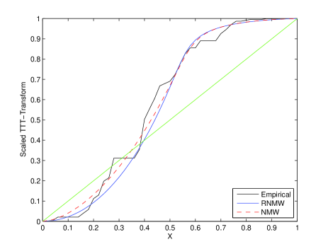
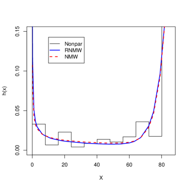
(c)	(d)

Figure 4: For Aarst data: (a) Histogram and fitted PDFs; (b) Empirical and fitted survival functions; (c) Empirical and fitted TTT-transforms; (c) Nonparametric and fitted hazard rate functions.

6.1.2 Kumar data

Kumar et al. [9] presented data consisting of times between failures (TBF) in days of load-haul-dump machines (LHD) used to pick up rock or waste. This data set also exhibits a bathtub shaped hazard rate function as shown in Figures 5c and 5d.

Tables 3 and 4 show the MLEs of the parameters, corresponding standard errors, AIC, BIC, CAIC and the K-S test statistics. Both distributions (NMW and RNMW) provide adequate fits. The log-likelihood is larger for the NMW distribution. That for the RNMW distribution is only slightly smaller. The K-S statistic is larger for the NMW distribution. However, the RNMW distribution has the smaller AIC, BIC and CAIC values.

Table 3: MLEs of parameters, standard errors, AIC, BIC and CAIC for Kumar data.

Model	$\widehat{\alpha}$	$\widehat{\beta}$	$\widehat{\gamma}$	$\widehat{\theta}$	$\widehat{\lambda}$	AIC	BIC	CAIC
NMW	$0.034$	$4.588\times 10^{-4}$	$0.423$	$0.657$	$0.071$	$410.0$	$418.9$	$411.6$
	(0.022)	($3.794\times 10^{-3}$)	(2.351)	(0.18)	(0.034)
RNMW	$0.055$	$5.852\times 10^{-4}$	$\frac{1}{2}$	$\frac{1}{2}$	$0.065$	$406.9$	$412.2$	$407.5$
	(0.017)	($6.523\times 10^{-4}$)	$-$	$-$	(0.012)

Table 4: K-S statistics for models fitted to Kumar data.

Model								K-S
NMW								0.068
RNMW								0.061

Figures 5a-d show that both distributions fit the data adequately. However, the log-likelihood ratio statistic for testing $H_{0}:\theta=\gamma=\frac{1}{2}$ versus $H_{1}:H_{0}$ is false is $\omega=0.895$ with the corresponding $p$-value of 0.639. Hence, again there is no evidence that the NMW distribution provides a better fit than the RNMW distribution.

The variance-covariance matrix for the fitted RNMW distribution is

$$I^{-1}=\left[\begin{array}[]{lll}2.839\times 10^{-4}&-3.968\times 10^{-6}&6.731\times 10^{-5}\\ -3.968\times 10^{-6}&4.254\times 10^{-7}&-7.836\times 10^{-6}\\ 6.731\times 10^{-5}&-7.836\times 10^{-6}&1.498\times 10^{-4}\end{array}\right].$$

So, approximate $95$ percent confidence intervals for the parameters $\alpha$, $\beta$ and $\lambda$ are $\left[0.022,0.088\right]$, $\left[0,1.864\times 10^{-3}\right]$ and $\left[0.041,0.089\right]$, respectively.

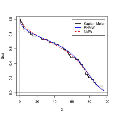
(a)	(b)
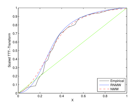
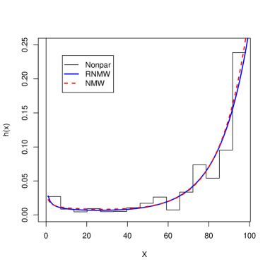
(c)	(d)

Figure 5: For Kumar data: (a) Histogram and fitted PDFs; (b) Empirical and fitted survival functions; (c) Empirical and fitted TTT-transforms; (c) Nonparametric and fitted hazard rate functions.

6.2 Censored data

In this section, we show how the RNMW distribution can be applied in practice for two real censored data sets, one of which is presented here for the first time.

6.2.1 Drug data

This data set was collected from a prison in the Middle East in 2011. It represents a sample of eighty two prisoners imprisoned for using or selling drugs. They were all released as part of a general amnesty for prisoners. We consider the time from release to reoffending to be the failure time. Of the eighty two prisoners, sixty six were arrested again for abuse or sale of drugs. After one hundred and eleven weeks, the others were considered to be censored.

Both the NMW and RNMW distributions were fitted to the data. Tables 5 and 6 show the MLEs of the parameters, corresponding standard errors, AIC, BIC, CAIC and the K-S test statistics. We see that the RNMW distribution has the smaller AIC, BIC and CAIC values. The K-S statistic values for both distributions are approximately equal to 0.055.

Figures 6a-d show the histogram of the data, PDFs of the fitted NMW and RNMW distributions, the empirical survival function, the survival functions of the fitted NMW and RNMW distributions, the empirical TTT-transform, TTT-transforms of the fitted NMW and RNMW distributions, the nonparametric hazard rate function, and the hazard rate functions of the fitted NMW and RNMW distributions. We can see that the RNMW distribution fits the data as well as the NMW distribution.

The log-likelihood ratio statistic for testing $H_{0}:\theta=\gamma=\frac{1}{2}$ versus $H_{1}:H_{0}$ is false is $\omega=1.496$ with the corresponding $p$-value of 0.473. Hence, again there is no evidence that the NMW distribution provides a better fit than the RNMW distribution.

Table 5: MLEs of parameters, standard errors, AIC, BIC and CAIC for drug data.

Model	$\widehat{\alpha}$	$\widehat{\beta}$	$\widehat{\gamma}$	$\widehat{\theta}$	$\widehat{\lambda}$	AIC	BIC	CAIC
NMW	0.019	$2.954\times 10^{-3}$	0.484	0.735	0.031	700.9	713.0	701.7
	($9.426\times 10^{-3}$)	$(3.656\times 10^{-3}$)	(0.504)	(0.159)	(0.019)
RNMW	0.038	$5.863\times 10^{-3}$	$\frac{1}{2}$	$\frac{1}{2}$	$0.026$	698.4	705.6	698.7
	(0.017)	($6.584\times 10^{-3}$)	$-$	$-$	($9.319\times 10^{-3}$)

Table 6: K-S statistics for models fitted to the drug data.

Model								K-S
NMW								0.0550
RNMW								0.0553

The variance-covariance matrix for the fitted RNMW distribution is

$$I^{-1}=\left[\begin{array}[]{lll}2.801\times 10^{-4}&-8.519\times 10^{-5}&1.138\times 10^{-4}\\ -8.519\times 10^{-5}&4.335\times 10^{-5}&-6.037\times 10^{-5}\\ 1.138\times 10^{-4}&-6.037\times 10^{-5}&8.684\times 10^{-5}\end{array}\right].$$

So, approximate $95$ percent confidence intervals for the parameters $\alpha$, $\beta$ and $\lambda$ are $\left[5.553\times 10^{-3},0.071\right]$, $\left[0,0.019\right]$ and $\left[8.137\times 10^{-3},0.045\right]$, respectively.

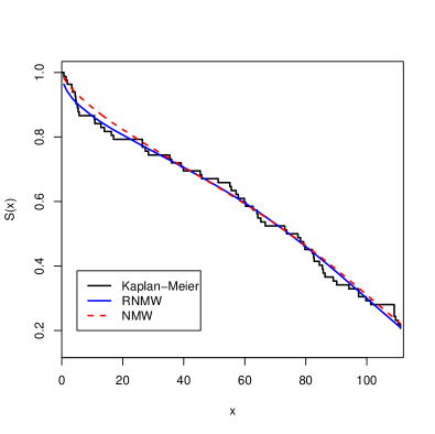
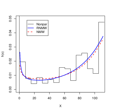
(a)	(b)

Figure 6: For drug data: (a) Histogram and fitted PDFs; (b) Empirical and fitted survival functions; (c) Empirical and fitted TTT-transforms; (c) Nonparametric and fitted hazard rate functions.

6.2.2 Serum-reversal data

Serum-reversal data consists of serum-reversal time in days of one hundred and forty eight children contaminated with HIV from vertical transmission at the university hospital of the Ribeirão Preto School of Medicine (Hospital das Clínicas da Faculdade de Medicina de Ribeirão Preto) from 1986 to 2001 [24], [17].

Tables 7 and 8 show the MLEs of the parameters, corresponding standard errors, AIC, BIC, CAIC and the K-S test statistics. We see that the RNMW distribution has smaller values for AIC, BIC and CAIC. The K-S statistic is only slightly larger for the NMW distribution.

Figures 7a-d show that both distributions fit the data adequately. However, the log-likelihood ratio statistic for testing $H_{0}:\theta=\gamma=\frac{1}{2}$ versus $H_{1}:H_{0}$ is false is $\omega=0.194$ with the corresponding $p$-value of 0.908. Hence, again there is no evidence that the NMW distribution provides a better fit than the RNMW distribution.

Table 7: MLEs of parameters, standard errors, AIC, BIC and CAIC for serum-reversal data.

Model	$\widehat{\alpha}$	$\widehat{\beta}$	$\widehat{\gamma}$	$\widehat{\theta}$	$\widehat{\lambda}$	AIC	BIC	CAIC
NMW	$1.74\times 10^{-3}$	$6.141\times 10^{-4}$	0.542	0.438	0.015	783.8	798.8	803.8
	($3.115\times 10^{-3}$)	$(2.274\times 10^{-3}$)	(0.507)	(0.763)	($3.764\times 10^{-3}$)
RNMW	$1.799\times 10^{-3}$	$5.955\times 10^{-4}$	$\frac{1}{2}$	$\frac{1}{2}$	$0.014$	780.1	789.1	792.1
	($1.971\times 10^{-3}$)	($4.174\times 10^{-4}$)	$-$	$-$	($2.061\times 10^{-3}$)

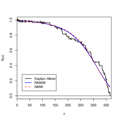
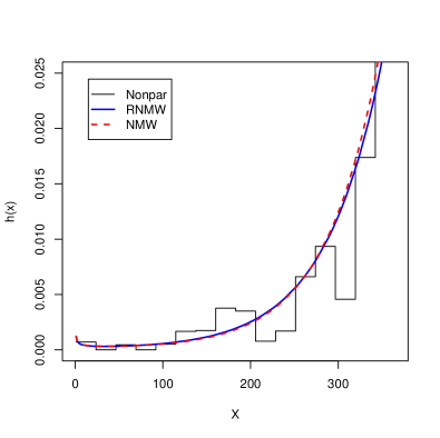
(a)	(b)

Figure 7: For serum data: (a) Histogram and fitted PDFs; (b) Empirical and fitted survival functions; (c) Empirical and fitted TTT-transforms; (c) Nonparametric and fitted hazard rate functions.

Table 8: K-S statistics for models fitted to serum-reversal data.

Model								K-S
NMW								0.115
RNMW								0.107

The variance-covariance matrix for the fitted RNMW distribution is

$$I^{-1}=\left[\begin{array}[]{lll}3.886\times 10^{-6}&-4.245\times 10^{-7}&1.990\times 10^{-6}\\ -4.245\times 10^{-7}&1.742\times 10^{-7}&-8.445\times 10^{-7}\\ 1.990\times 10^{-6}&-8.445\times 10^{-7}&4.246\times 10^{-6}\end{array}\right].$$

So, approximate $95$ percent confidence intervals for the parameters $\alpha$, $\beta$ and $\lambda$ are $\left[0,5.662\times 10^{-3}\right]$, $\left[0,1.414\times 10^{-3}\right]$ and $\left[0.010,0.080\right]$, respectively.

7 Conclusions and further discussion

The NMW distribution introduced by Almalki and Yuan [2] has been simplified with its five parameters reduced to three. The simplified distribution has been referred to as the RNMW distribution. We have studied several analytical properties of the RNMW distribution and shown it to be a tractable distribution. We have also shown that the RNMW distribution provides excellent fits to four real data sets: two of them are complete data sets and the other two are censored. By means of the likelihood ratio test, we have shown that the fit of the NMW distribution is not significantly better than that of the RNMW distribution. So, the RNMW distribution retains the same flexibility of the NMW distribution and yet the estimation for the former is much easier.

The RNMW distribution has an exclusive bathtub shaped hazard rate function. Other hazard rates can be obtained from the NMW distribution. For example, setting $\gamma=\theta=2$ we obtain

$$h(x)=2\alpha x+\beta(2+\lambda x)xe^{\lambda x}$$

for $x>0$, which is an increasing function of $x$, see Figure 8.

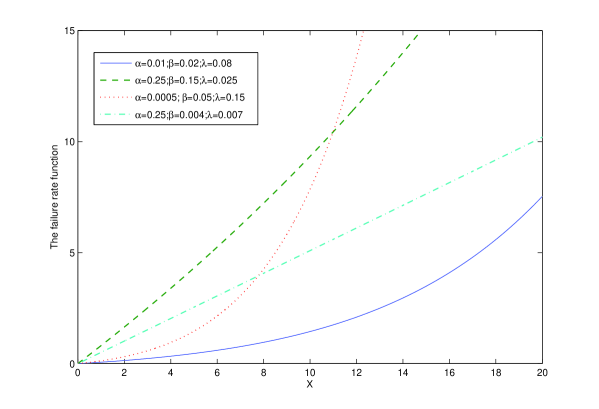
Figure 8: Hazard rate functions of the reduced distribution.

Appendix A Appendix

The moment generating function of $X$ is

$$M_{X}(t) = E\left(e^{tx}\right)$$

$$= \int_{0}^{\infty}e^{tx}f(x)dx$$

$$= \int_{0}^{\infty}e^{tx}dF(x)$$

$$= 1+\int_{0}^{\infty}te^{tx}e^{-\alpha\sqrt{x}-\beta\sqrt{x}e^{\lambda x}}dx$$

$$= 1+\sum_{n,m,k=0}^{\infty}\frac{(-\beta)^{n}(n\lambda)^{m}t^{k+1}}{i!j!k!}I,$$

where $I=\int_{0}^{\infty}x^{\frac{n}{2}+m+k}e^{-\alpha\sqrt{x}}dx$. Using gamma-integral formula, we obtain

$$M_{X}(t)=1+2\sum_{n,m,k=0}^{\infty}\frac{(-\beta)^{n}(n\lambda)^{m}t^{k+1}}{i!j!k!}\left[\frac{\Gamma\left(n+2(m+k)+2\right)}{\alpha^{n+2(m+k)+2}}\right].$$

Appendix B Appendix

The elements of the observed information matrix $I(\vartheta)$ for the $RNMW(\alpha,\beta,\lambda)$ for complete data are

$$\ell_{\alpha\alpha}=-\sum\limits_{i=1}^{d}\left[\frac{h_{\alpha}\left(x_{i};\underline{\vartheta}\right)}{h\left(x_{i};\underline{\vartheta}\right)}\right]^{2},$$

$$\ell_{\alpha\beta}=-\sum\limits_{i=1}^{d}\frac{h_{\alpha}\left(x_{i};\underline{\vartheta}\right)h_{\beta}\left(x_{i};\underline{\vartheta}\right)}{h\left(x_{i};\underline{\vartheta}\right)^{2}},$$

$$\ell_{\alpha\lambda}=-\sum\limits_{i=1}^{d}\frac{h_{\alpha}\left(x_{i};\underline{\vartheta}\right)h_{\lambda}\left(x_{i};\underline{\vartheta}\right)}{h\left(x_{i};\underline{\vartheta}\right)^{2}},$$

$$\ell_{\beta\beta}=-\sum\limits_{i=1}^{d}\left[\frac{h_{\beta}\left(x_{i};\underline{\vartheta}\right)}{h\left(x_{i};\underline{\vartheta}\right)}\right]^{2},$$

$$\ell_{\beta\lambda}=-\sum\limits_{i=1}^{d}\frac{h\left(x_{i};\underline{\vartheta}\right)h_{\beta\lambda}\left(x_{i};\underline{\vartheta}\right)-h_{\beta}\left(x_{i};\underline{\vartheta}\right)h_{\lambda}\left(x_{i};\underline{\phi}\right)}{h\left(x_{i};\underline{\vartheta}\right)^{2}},$$

$$\ell_{\lambda\lambda}=\sum\limits_{i=1}^{d}\left[\frac{h\left(x_{i};\underline{\vartheta}\right)h_{\lambda\lambda}\left(x_{i};\underline{\vartheta}\right)-h_{\lambda}\left(x_{i};\underline{\vartheta}\right)^{2}}{h\left(x_{i};\underline{\vartheta}\right)^{2}}-\beta\sqrt{x_{i}^{5}}e^{\lambda x_{i}}\right],$$

where

$$h_{\alpha}\left(x_{i};\underline{\vartheta}\right)=\frac{1}{2\sqrt{x_{i}}},$$

$$h_{\beta}\left(x_{i};\underline{\vartheta}\right)=\frac{\left(0.5+\lambda x_{i}\right)e^{\lambda x_{i}}}{\sqrt{x_{i}}},$$

$$h_{\lambda}\left(x_{i};\underline{\vartheta}\right)=\beta\sqrt{x_{i}}\left(\frac{3}{2}+\lambda x_{i}\right)e^{\lambda x_{i}},$$

$$h_{\beta\lambda}\left(x_{i};\underline{\vartheta}\right)=\sqrt{x_{i}}\left(\frac{3}{2}+\lambda x_{i}\right)e^{\lambda x_{i}},$$

$$h_{\lambda\lambda}\left(x_{i};\underline{\vartheta}\right)=\beta\sqrt{x_{i}}\left(\frac{5}{2}+\lambda x_{i}\right)e^{\lambda x_{i}}.$$

Appendix C Appendix

The elements of the observed information matrix $I(\vartheta)$ for the $RNMW(\alpha,\beta,\lambda)$ for censored data are

$$I_{\alpha\alpha}=-\sum\limits_{i=1}^{d}\left[\frac{h_{\alpha}\left(x_{i};\underline{\vartheta}\right)}{h\left(x_{i};\underline{\vartheta}\right)}\right]^{2},$$

$$I_{\alpha\beta}=-\sum\limits_{i=1}^{d}\frac{h_{\alpha}\left(x_{i};\underline{\vartheta}\right)h_{\beta}\left(x_{i};\underline{\vartheta}\right)}{h\left(x_{i};\underline{\vartheta}\right)^{2}},$$

$$I_{\alpha\lambda}=-\sum\limits_{i=1}^{d}\frac{h_{\alpha}\left(x_{i};\underline{\vartheta}\right)h_{\lambda}\left(x_{i};\underline{\vartheta}\right)}{h\left(x_{i};\underline{\vartheta}\right)^{2}},$$

$$I_{\beta\beta}=-\sum\limits_{i=1}^{d}\left[\frac{h_{\beta}\left(x_{i};\underline{\vartheta}\right)}{h\left(x_{i};\underline{\vartheta}\right)}\right]^{2},$$

$$I_{\beta\lambda}=-\sum\limits_{i=1}^{d}\frac{h\left(x_{i};\underline{\vartheta}\right)h_{\beta\lambda}\left(x_{i};\underline{\vartheta}\right)-h_{\beta}\left(x_{i};\underline{\vartheta}\right)h_{\lambda}\left(x_{i};\underline{\phi}\right)}{h\left(x_{i};\underline{\vartheta}\right)^{2}}-\sum\limits_{i\in C}\sqrt{x_{i}^{3}}e^{\lambda x_{i}},$$

$$I_{\lambda\lambda}=\sum\limits_{i=1}^{d}\left[\frac{h\left(x_{i};\underline{\vartheta}\right)h_{\lambda\lambda}\left(x_{i};\underline{\vartheta}\right)-h_{\lambda}\left(x_{i};\underline{\vartheta}\right)^{2}}{h\left(x_{i};\underline{\vartheta}\right)^{2}}-\beta\sqrt{x_{i}^{5}}e^{\lambda x_{i}}\right]$$

$$\qquad\qquad-\beta\sum\limits_{i\in C}\sqrt{x_{i}^{5}}e^{\lambda x_{i}},$$

where

$$h_{\alpha}\left(x_{i};\underline{\vartheta}\right)=\frac{1}{2\sqrt{x_{i}}},$$

$$h_{\beta}\left(x_{i};\underline{\vartheta}\right)=\frac{\left(0.5+\lambda x_{i}\right)e^{\lambda x_{i}}}{\sqrt{x_{i}}},$$

$$h_{\lambda}\left(x_{i};\underline{\vartheta}\right)=\beta\sqrt{x_{i}}\left(\frac{3}{2}+\lambda x_{i}\right)e^{\lambda x_{i}},$$

$$h_{\beta\lambda}\left(x_{i};\underline{\vartheta}\right)=\sqrt{x_{i}}\left(\frac{3}{2}+\lambda x_{i}\right)e^{\lambda x_{i}},$$

$$h_{\lambda\lambda}\left(x_{i};\underline{\vartheta}\right)=\beta\sqrt{x_{i}^{3}}\left(\frac{5}{2}+\lambda x_{i}\right)e^{\lambda x_{i}}.$$

References

- [1] Aarset, M. V. (1987). How to identify bathtub hazard rate. IEEE Transactions on Reliability, R-36, 106-108.
- [2] Almalki, S. J. and Yuan, J. (2013). The new modified Weibull distribution. Reliability Engineering and System Safety, 111, 164-170.
- [3] Bain, L. J. (1974). Analysis for the linear failure-rate life-testing distribution. Technometrics, 16, 551-559.
- [4] Bebbington, M., Lai, C. D. and Zitikis, R. (2007). A flexible Weibull extension. Reliability Engineering and System Safety, 92, 719-726.
- [5] Carrasco, M., Ortega, E. M. and Cordeiro, G. M. (2008). A generalized modified Weibull distribution for lifetime modeling. Computational Statistics and Data Analysis, 53, 450-462.
- [6] Cordeiro, G. M., Ortega, E. M. and Nadarajah, S. (2010). The Kumaraswamy Weibull distribution with application to failure data. Journal of the Franklin Institute, 347, 1399-1429.
- [7] Famoye, F., Lee, C. and Olumolade, O. (2005). The beta-Weibull distribution. Journal of Statistical Theory and Applications, 4, 121-136.
- [8] Kies, J. A. (1958). The strength of glass. Naval Research Laboratory Report No. 5093, Washington D.C.
- [9] Kumar, U., Klefsjö, B. and Granholm, S. (1989). Reliability investigation for a fleet of load haul dump machines in a Swedish mine. Reliability Engineering and System Safety, 26, 341-361.
- [10] Kuo, W. and Zuo, M. J. (2001). Optimal Reliability Modeling: Principles and Applications. John Wiley and Sons, New York.
- [11] Lai, C. D., Murthy, D. N. P. and Xie, M. (2011). Weibull distributions. Computational Statistics, 33, 282-287.
- [12] Lai, C. D., Xie, M., and Murthy, D. N. P. (2003). A modified Weibull distribution. IEEE Transactions on Reliability, 52, 33-37.
- [13] Meeker, W. Q. and Escobar, L. A. (1998). Statistical Methods for Reliability Data. John Wiley and Sons, New York.
- [14] Miller, R. G., Gong, G. and Muñoz, A. (1981). Survival Analysis. John Wiley and Sons, New York.
- [15] Murthy, D. N. P., Xie, M. and Jiang, R. (2003). Weibull Models. John Wiley and Sons, New York.
- [16] Nelson, W. (1990). Accelerated Testing: Statistical Models, Test Plans, and Data Analysis. John Wiley and Sons, New York.
- [17] Perdoná, G. S. C. (2006). Modelos de Riscos Aplicados à Análise de Sobrevivência (in Portuguese). Doctoral Thesis, Institute of Computer Science and Mathematics, University of São Paulo, Brasil.
- [18] Pham, H. and Lai, C. D. (2007). On recent generalizations of the Weibull distribution. IEEE Transactions on Reliability, 56, 454-458.
- [19] Phani, K. K. (1987). A new modified Weibull distribution function. Communications of the American Ceramic Society, 70, 182-184.
- [20] Rajarshi, S. and Rajarshi, M. B. (1988). Bathtub distributions: A review. Communications in Statistics-Theory and Methods, 17, 2597-2621.
- [21] Sarhan, A. M., Abd El-Baset, A. A. and Alasbahi, I. A. (2013). Exponentiated generalized linear exponential distribution. Applied Mathematical Modeling, 37, 2838-2849.
- [22] Sarhan, A. M. and Apaloo, J. (2013). Exponentiated modified Weibull extension distribution. Reliability Engineering and System Safety, 112, 137-144.
- [23] Sarhan, A. M. and Zaindin, M. (2009). Modified Weibull distribution. Applied Sciences, 11, 123-136.
- [24] Silva, A. N. F. (2004). Estudo evolutivo das crianças expostas ao HIV e notificadas pelo núcleo de vigilância epidemiológica do HCFMRP-USP (in Portuguese). M.Sc. Thesis, University of São Paulo, Brasil.
- [25] Silva, G. O., Ortega, E. M. and Cordeiro, G. M. (2010). The beta modified Weibull distribution. Lifetime Data Analysis, 16, 409-430.
- [26] Singla, N., Jain, K. and Kumar Sharma, S. (2012). The beta generalized Weibull distribution: Properties and applications. Reliability Engineering and System Safety, 102, 5-15.
- [27] Weibull, W. A. (1951). Statistical distribution function of wide applicability. Journal of Applied Mechanics, 18, 293-296.
- [28] Xie, M. and Lai, C. D. (1995). Reliability analysis using an additive Weibull model with bathtub-shaped failure rate function. Reliability Engineering and System Safety, 52, 87-93.
- [29] Xie, M., Tang, Y. and Goh, T. N. (2002). A modified Weibull extension with bathtub-shaped failure rate function. Reliability Engineering and System Safety, 76, 279-285.