Pebble Games, Proof Complexity,
and Time-Space Trade-offs*

Abstract.

Pebble games were extensively studied in the 1970s and 1980s in a number of different contexts. The last decade has seen a revival of interest in pebble games coming from the field of proof complexity. Pebbling has proven to be a useful tool for studying resolution-based proof systems when comparing the strength of different subsystems, showing bounds on proof space, and establishing size-space trade-offs. This is a survey of research in proof complexity drawing on results and tools from pebbling, with a focus on proof space lower bounds and trade-offs between proof size and proof space.

Pebbling and Proof Complexity

In this section, we describe the connections between pebbling and proof complexity that is the main motivation behind this survey. Our focus will be on how pebble games have been employed to study trade-offs between time and space in resolution-based proof systems, in particular in the line of work [Nor09a, NH13, BN08, BN11], but we will also discuss other usages of pebbling in proof complexity. Let us start, however, by giving a quick overview of proof complexity in general.

1. A Selective Introduction to Proof Complexity

Ever since the fundamental NP-completeness result of Stephen Cook [Coo71], the problem of deciding whether a given propositional logic formula in conjunctive normal form (CNF) is satisfiable or not has been on center stage in Theoretical Computer Science. In more recent years, satisfiability has gone from a problem of mainly theoretical interest to a practical approach for solving applied problems. Although all known Boolean satisfiability solvers (SAT solvers) have exponential running time in the worst case, enormous progress in performance has led to satisfiability algorithms becoming a standard tool for solving a large number of real-world problems such as hardware and software verification, experiment design, circuit diagnosis, and scheduling.

Perhaps a somewhat surprising aspect of this development is that the most successful SAT solvers to date are still variants of the Davis-Putnam-Logemann-Loveland (DPLL) procedure [DLL62, DP60] augmented with clause learning [BS97, MS99], which can be seen to search for proofs in the resolution proof system. For instance, the great majority of the best algorithms in recent rounds of the international SAT competition [SAT] fit this description.

DPLL procedures perform a recursive backtrack search in the space of partial truth value assignments. The idea behind clause learning is that at each failure (backtrack) point in the search tree, the system derives a reason for the inconsistency in the form of a new clause and then adds this clause to the original CNF formula (“learning” the clause). This can save much work later on in the proof search, when some other partial truth value assignment fails for similar reasons.

The main bottleneck for this approach, other than the obvious one that the running time is known to be exponential in the worst case, is the amount of space used by the algorithms. Since there is only a fixed amount of memory, all clauses cannot be stored. The difficulty lies in obtaining a highly selective and efficient clause caching scheme that nevertheless keeps the clauses needed. Thus, understanding time and memory requirements for clause learning algorithms, and how these requirements are related to each other, is a question of great practical importance.

Some good papers discussing clause learning (and SAT solving in general) with examples of applications are [BKS04, KS07, Mar08]. A more exhaustive general reference is the recently published Handbook of Satisfiability [BHvMW09]. The first chapter of this handbook provides an excellent historical overview of the satisfiability problem, with pages 19–25 focusing in particular on DPLL and resolution.

The study of proof complexity originated with the seminal paper of Cook and Reckhow [CR79]. In its most general form, a proof system for a language $L$ is a binary predicate $P(x,\pi)$, which is computable (deterministically) in time polynomial in the sizes $\lvert x\rvert$ and $\lvert\pi\rvert$ of the input and has the property that for all $x\in L$ there is a string $\pi$ (a proof) for which $P(x,\pi)$ evaluates to true, whereas for any $x\not\in L$ it holds for all strings $\pi$ that $P(x,\pi)$ evaluates to false. A proof system is said to be polynomially bounded if for every $x\in L$ there exists a proof $\pi_{x}$ for $x$ that has size at most polynomial in $\lvert x\rvert$. A propositional proof system is a proof system for the language of tautologies in propositional logic.

From a theoretical point of view, one important motivation for proof complexity is the intimate connection with the fundamental question of P versus NP. Since NP is exactly the set of languages with polynomially bounded proof systems, and since tautology can be seen to be the dual problem of satisfiability, we have the famous theorem of [CR79] that NP = co-NP if and only if there exists a polynomially bounded propositional proof system. Thus, if it could be shown that there are no polynomially bounded proof systems for propositional tautologies, P $\neq$ NP would follow as a corollary since P is closed under complement. One way of approaching this distant goal is to study stronger and stronger proof systems and try to prove superpolynomial lower bounds on proof size. However, although great progress has been made in the last couple of decades for a variety of propositional proof systems, it seems that we still do not fully understand the reasoning power of even quite simple ones.

Another important motivation for proof complexity is that, as was mentioned above, designing efficient algorithms for proving tautologies (or, equivalently, testing satisfiability) is a very important problem not only in the theory of computation but also in applied research and industry. All automated theorem provers, regardless of whether they produce a written proof or not, explicitly or implicitly define a system in which proofs are searched for and rules which determine what proofs in this system look like. Proof complexity analyzes what it takes to simply write down and verify the proofs that such an automated theorem prover might find, ignoring the computational effort needed to actually find them. Thus, a lower bound for a proof system tells us that any algorithm, even an optimal (non-deterministic) one making all the right choices, must necessarily use at least the amount of a certain resource specified by this bound. In the other direction, theoretical upper bounds on some proof complexity measure give us hope of finding good proof search algorithms with respect to this measure, provided that we can design algorithms that search for proofs in the system in an efficient manner. For DPLL procedures with clause learning, also known as conflict-driven clause learning (CDCL) solvers, the time and memory resources used are measured by the length and space of proofs in the resolution proof system.

The field of proof complexity also has rich connections to cryptography, artificial intelligence and mathematical logic. We again refer the reader to, for instance, [Bea04, BP98, CK02, Seg07, Urq95] for more information.

1.1. Resolution-Based Proof Systems

Any formula in propositional logic can be converted to a CNF formula that is only linearly larger and is unsatisfiable if and only if the original formula is a tautology. Therefore, any sound and complete system that certifies the unsatisfiability of CNF formulas can be considered as a general propositional proof system.

Arguably the single most studied proof system in propositional proof complexity, resolution, is such a system that produces proofs of the unsatisfiability of CNF formulas. The resolution proof system appeared in [Bla37] and began to be investigated in connection with automated theorem proving in the 1960s [DLL62, DP60, Rob65]. Because of its simplicity—there is only one derivation rule—and because all lines in a proof are disjunctive clauses, this proof system readily lends itself to proof search algorithms.

Being so simple and fundamental, resolution was also a natural target to attack when developing methods for proving lower bounds in proof complexity. In this context, it is most straightforward to prove bounds on the length of refutations, i.e., the number of clauses, rather than on the size of refutations, i.e., the total number of symbols. The length and size measures are easily seen to be polynomially related. The first superpolynomial lower bound on resolution was presented by Tseitin in the paper [Tse68], which is the published version of a talk given in 1966, for a restricted form of the proof system called regular resolution. It took almost an additional 20 years before Haken [Hak85] was able to establish superpolynomial bounds without any restrictions, showing that CNF encodings of the pigeonhole principle are intractable for general resolution. This weakly exponential bound of Haken has later been followed by many other strong results, among others truly exponential lower bounds on resolution refutation length for different formula families in, for instance, [BKPS02, BW01, CS88, Urq87].

A second complexity measure for resolution, first made explicit by Galil [Gal77], is the width, measured as the maximal size of a clause in the refutation. Clearly, the maximal width needed to refute any unsatisfiable CNF formula is at most the number of variables in it, which is upper-bounded by the formula size. Hence, while refutation length can be exponential in the worst case, the width ranges between constant and linear measured in the formula size. Inspired by previous work [BP96, CEI96, IPS99], Ben-Sasson and Wigderson [BW01] identified width as a crucial resource of resolution proofs by showing that the minimal width of any resolution refutation of a $k$-CNF formula ${F}$ (i.e., a formula where all clauses have size at most some constant $k$) is bounded from above by the minimal refutation length by

$$\text{minimal width}\leq\mathrm{O}\bigl{(}\sqrt{(\text{size of formula})\cdot\log(\text{minimal length})}\bigr{)}.$$ (1)

Since it is also easy to see that resolution refutations of polynomial-size formulas in small width must necessarily be short—quite simply for the reason that $(2\cdot\#\text{variables})^{w}$ is an upper bound on the total number of distinct clauses of width at most $w$—the result in [BW01] can be interpreted as saying roughly that there exists a short refutation of the $k$-CNF formula ${F}$ if and only if there exists a (reasonably) narrow refutation of ${F}$. This interpretation also gives rise to a natural proof search heuristic: to find a short refutation, search for refutations in small width. It was shown in [BIW04] that there are formula families for which this heuristic exponentially outperforms any DPLL procedure (without clause learning) regardless of branching function.

The idea to study space in the context of proof complexity appears to have been raised for the first time by Armin Haken during a workshop in Toronto in 1998, and the formal study of space in resolution was initiated by Esteban and Torán in [ET01] and was later extended to a more general setting by Alekhnovich et al.in [ABRW02]. Intuitively, we can view a resolution refutation of a CNF formula ${F}$ as a sequence of derivation steps on a blackboard, where in each step we may write a clause from ${F}$ on the blackboard, erase a clause from the blackboard, or derive some new clause implied by the clauses currently written on the blackboard, and where the refutation ends when we reach the contradictory empty clause. The space of a refutation is then the maximal number of clauses one needs to keep on the blackboard simultaneously at any time during the refutation, and the space of refuting ${F}$ is defined as the minimal space of any resolution refutation of ${F}$. A number of upper and lower bounds for refutation space in resolution and other proof systems were subsequently presented in, for example, [ABRW02, BG03, EGM04, ET03], and to distinguish the space measure of [ET01] from other measures introduced in these later papers we will sometimes refer to it as clause space below for extra clarity.

Just as is the case for width, the minimum clause space of refuting a formula can be upper-bounded by the formula size. Somewhat unexpectedly, it was discovered in a sequence of works that lower bounds on resolution refutation space for different formula families turned out to match exactly previously known lower bounds on refutation width. In an elegant paper [AD08], Atserias and Dalmau showed that this was not a coincidence, but that the inequality

$$\text{minimal width}\leq\text{minimal clause space}+\text{small constant}$$ (2)

holds for refutations of any $k$-CNF formula ${F}$, where the constant term depends only on $k$. Since clause space is an upper bound on width by (2), and since width upper-bounds length by the counting argument discussed above, it follows that upper bounds on clause space imply upper bounds on length. Esteban and Torán [ET01] showed the converse that length upper bounds imply clause space upper bounds for the restricted case of tree-like resolution (where every clause can only be used once in the derivation and has to be rederived again from scratch if it is needed again at some later stage in the proof). Thus, clause space is an interesting complexity measure with nontrivial relations to proof length and width. We note that apart from being of theoretical interest, clause space has also been proposed in [ABLM08] as a relevant measure of the hardness in practice of CNF formulas for SAT solvers, and such possible connections have been further investigated in [JMNŽ12].

The resolution proof system was generalized by Krajíček [Kra01], who introduced the the family of $k$-DNF resolution proof systems as an intermediate step between resolution and depth-$2$ Frege systems. Roughly speaking, for positive integers $k$ the $k$th member of this family, which we denote $\mathcal{R}({k})$, is allowed to reason in terms of formulas in disjunctive normal form (DNF formulas) with the added restriction that any conjunction in any formula is over at most $k$ literals. For $k=1$, the lines in the proof are hence disjunctions of literals, and the system $\mathcal{R}({1})=\mathcal{R}$ is standard resolution. At the other extreme, $\mathcal{R}({\infty})$ is equivalent to depth-$2$ Frege.

The original motivation to study the family of $k$-DNF resolution proof systems, as stated in [Kra01], was to better understand the complexity of counting in weak models of bounded arithmetic, and it was later observed that these systems are also related to SAT solvers that reason using multi-valued logic (see [JN02] for a discussion of this point). A number of subsequent works have shown superpolynomial lower bounds on the length of $\mathcal{R}({k})$-refutations, most notably for (various formulations of) the pigeonhole principle and for random CNF formulas [AB04, ABE02, Ale11, JN02, Raz03, SBI04, Seg05]. Of particular interest in the current context are the results of Segerlind et al. [SBI04] and of Segerlind [Seg05] showing that the family of $\mathcal{R}({k})$-systems form a strict hierarchy with respect to proof length. More precisely, they prove that for every $k$ there exists a family of formulas $\{F_{n}\}_{n=1}^{\infty}$ of arbitrarily large size $n$ such that $F_{n}$ has an $\mathcal{R}({k+1})$-refutation of polynomial length but any $\mathcal{R}({k})$-refutation of $F_{n}$ requires exponential length.

With regard to space, Esteban et al. [EGM04] established essentially optimal linear lower bounds in $\mathcal{R}({k})$ on formula space, extending the clause space measure for resolution in the natural way by counting the number of $k$-DNF formulas. They also proved that the family of tree-like $\mathcal{R}({k})$ systems form a strict hierarchy with respect to formula space in the sense that there are arbitrarily large formulas $F_{n}$ of size $n$ that can be refuted in tree-like $\mathcal{R}({k+1})$ in constant space but require space $\Omega(n/\log^{2}n)$ to be refuted in tree-like $\mathcal{R}({k})$. It should be pointed out, however, that as observed in [Kra01, EGM04] the family of tree-like $\mathcal{R}({k})$ systems for all $k>0$ are strictly weaker than standard resolution. As was mentioned above, the family of general, unrestricted $\mathcal{R}({k})$ systems are strictly stronger than resolution, so the results in [EGM04] left open the question of whether there is a strict formula space hierarchy for (non-tree-like) $\mathcal{R}({k})$ or not.

1.2. Three Questions Regarding Space

Although resolution is simple and by now very well-studied, the research surveyed above left open a few fundamental questions about this proof system. In what follows, our main focus will be on the three questions considered below.

1. What is the relation between clause space and width? The inequality (2) says that clause space $\gtrapprox$ width, but it leaves open whether this relationship is tight or not. Do the clause space and width measures always coincide, or is there a formula family that separates the two measures asymptotically?

2. What is the relation between clause space and length? Is there some nontrivial correlation between the two in the sense that formulas refutable in short length must also be refutable in small space, or can “easy” formulas with respect to length be “arbitrarily complex” with respect to space? (We will make these notions more precise shortly.)

3. Can the length and space of refutations be optimized simultaneously, or are there trade-offs in the sense that any refutation that optimizes one of the two measures must suffer a blow-up in the other?

To put the questions about length versus space in perspective, consider what has been known for length versus width. It follows from the inequality (1) that if the width of refuting a $k$-CNF formula family $\{{F}_{n}\}_{n=1}^{\infty}$ of size $n$ grows asymptotically faster than $\sqrt{n\log n}$, then the length of refuting ${F}_{n}$ must be superpolynomial. This is known to be almost tight, since Bonet and Galesi [BG01] showed that there is a family of $k$-CNF formulas of size $n$ with minimal refutation width growing like $\sqrt[3]{n}$, but which is nevertheless refutable in length linear in $n$. Hence, formulas refutable in polynomial length can have somewhat wide minimum-width refutations, but not arbitrarily wide ones.

Turning to the relation between clause space and length, we note that the inequality (2) tells us that any correlation between length and clause space cannot be tighter than the correlation between length and width. In particular, we get from the previous paragraph that $k$-CNF formulas refutable in polynomial length may have at least “somewhat spacious” minimum-space refutations. At the other end of the spectrum, given any resolution refutation of ${F}$ in length ${\mathit{L}}$ it is a straightforward consequence of [ET01, HPV77] that the space needed to refute ${F}$ is at most on the order of ${\mathit{L}}/\log{\mathit{L}}$. This gives a trivial upper bound on any possible separation of the two measures. Thus, what the question above is asking is whether it can be that length and space are “completely unrelated” in the sense that there exist $k$-CNF formulas with refutation length ${\mathit{L}}$ that need maximum possible space $\Omega\bigl{(}L/\log L\bigr{)}$, or whether there is a nontrivial upper bound on clause space in terms of length analogous to the inequality in (1), perhaps even stating that $\text{minimal clause space}\leq\mathrm{O}\bigl{(}\sqrt{(\text{size of formula})\cdot\log(\text{minimal length})}\bigr{)}$ or similar. Intriguingly, as we discussed above it was shown in [ET01] that for the restricted case of so-called tree-like resolution there is in fact a tight correspondence between length and clause space, exactly as for length versus width.

1.3. Pebble Games to the Rescue

Although the above questions have been around for a while, as witnessed by discussions in, for instance, the papers [ABRW02, Ben09, BG03, EGM04, ET03, Seg07, Tor04], there appears to have been no consensus on what the right answers should be. However, what most of these papers did agree on was that a plausible formula family for answering these questions were so-called pebbling contradictions, which are CNF formulas encoding pebble games played on graphs. Pebbling contradictions had already appeared in various disguises in some of the papers mentioned in Section 1.1, and it had been noted that non-constant lower bounds on the clause space of refuting pebbling contradictions would separate space and width and possibly also clarify the relation between space and length if the bounds were good enough. On the other hand, a constant upper bound on the refutation space would improve the trade-off results for different proof complexity measures for resolution in [Ben09].

And indeed, pebbling turned out to be just the right tool to understand the interplay of length and space in resolution. The main purpose of this section is to give an overview of the works establishing connections between pebbling and proof complexity with respect to time-space trade-offs. We will need to give some preliminaries in order to state the formal results, but before we do so let us conclude this introduction by giving a brief description of the relevant results.

The first progress was reported in 2006 (journal version in [Nor09a]), where pebbling formulas of a very particular form, namely pebbling contradictions defined over complete binary trees, were studied. This was sufficient to establish a logarithmic separation of clause space and width, thus answering question 1 above. This separation was improved from logarithmic to polynomial in 2008 (journal version in [NH13]), where a broader class of graphs were analyzed, but where unfortunately a rather involved argument was required for this analysis to go through. In [BN08], a somewhat different approach was taken by modifying the pebbling formulas slightly. This made the analysis both much simpler and much stronger, and led to a resolution of question 2 by establishing an optimal separation between clause space and length, i.e., showing that there are formulas with refutation length ${\mathit{L}}$ that require clause space $\Omega\bigl{(}L/\log L\bigr{)}$. In a further improvement, the paper [BN11] used similar ideas to translate pebbling time-space trade-offs to trade-offs between length and space in resolution, thus answering question 3. In the same paper these results were also extended to the $k$-DNF resolution proof systems, which also yielded as a corollary that the $\mathcal{R}({k})$-systems indeed form a strict hierarchy with respect to space.

2. Proof Complexity Preliminaries

Below we present the definitions, notation and terminology that we will need to make more precise the informal exposition in Section 1.

2.1. Variables, Literals, Terms, Clauses, Formulas and Truth Value Assignments

For $x$ a Boolean variable, a literal over $x$ is either the variable $x$ itself, called a positive literal over $x$, or its negation, denoted $\lnot x$ or $\overline{x}$ and called a negative literal over $x$. Sometimes it will also be convenient to write $x^{1}$ for unnegated variables and $x^{0}$ for negated ones. We define $\lnot\lnot x$ to be $x$. A clause $C=a_{1}\lor\cdots\lor a_{k}$ is a disjunction of literals, and a term $T=a_{1}\land\cdots\land a_{k}$ is a conjunction of literals. Below we will think of clauses and terms as sets, so that the ordering of the literals is inconsequential and that, in particular, no literals are repeated. We will also (without loss of generality) assume that all clauses and terms are nontrivial in the sense that they do not contain both a literal and its complement. A clause (term) containing at most $k$ literals is called a $k$-clause ($k$-term). A CNF formula ${F}=C_{1}\land\cdots\land C_{m}$ is a conjunction of clauses, and a DNF formula is a disjunction of terms. We will think of CNF and DNF formulas as sets of clauses and terms, respectively. A $k$-CNF formula is a CNF formula consisting of $k$-clauses, and a $k$-DNF formula consists of $k$-terms.

The variable set of a clause $C$, denoted $\mathit{Vars}({C})$, is the set of Boolean variables over which there are literals in $C$, and we write $\mathit{Lit}({C})$ to denote the set of literals in $C$. The variable and literal sets of a term are similarly defined and these definitions are extended to CNF and DNF formulas by taking unions. If $V$ is a set of Boolean variables and $\mathit{Vars}({C})\subseteq V$, we say $C$ is a clause over $V$ and similarly define terms, CNF formulas, and DNF formulas over $V$.

In what follows, we will usually write $a,b,c$ to denote literals, $A,B,C,D$ to denote clauses, $T$ to denote terms, ${F},{G}$ to denote CNF formulas, and $\mathbb{C},\mathbb{D}$ to denote sets of clauses, $k$-DNF formulas or sometimes other Boolean functions. We will assume the existence of an arbitrary but fixed set of variables $V=\{x,y,z,\ldots\}$. For a variable $x\in V$ we define $\mathit{Vars}^{d}({x})=\{x_{1},\ldots,x_{d}\}$, and we will tacitly assume that $V$ is such that the new set of variables $\mathit{Vars}^{d}({V})=\{x_{1},\ldots,x_{d},y_{1},\ldots,y_{d},z_{1},\ldots,z_{d},\ldots\}$ is disjoint from $V$. We will say that the variables $x_{1},\ldots,x_{d}$, and any literals over these variables, all belong to the variable $x$.

We write ${\alpha},{\beta}$ to denote truth value assignments, usually over $\mathit{Vars}^{d}({V})$ but sometimes over $V$. Partial truth value assignments, or restrictions, will often be denoted $\rho$. Truth value assignments are functions to $\{0,1\}$, where we identify $0$ with false and $1$ with true. We have the usual semantics that a clause is true under ${\alpha}$, or satisfied by ${\alpha}$, if at least one literal in it is true, and a term is true if all literals evaluate to true. We write $\bot$ to denote the empty clause without literals that is false under all truth value assignments. (The empty clause is also denoted, for instance, $\lambda$, $\Lambda$, or $\{\}$ in the literature.) A CNF formula is satisfied if all clauses in it are satisfied, and for a DNF formula we require that some term should be satisfied. In general, we will not distinguish between a formula and the Boolean function computed by it.

If $\mathbb{C}$ is a set of Boolean functions we say that a restriction (or assignment) satisfies $\mathbb{C}$ if and only if it satisfies every function in $\mathbb{C}$. For $\mathbb{D},\mathbb{C}$ two sets of Boolean functions over a set of variables $V$, we say that $\mathbb{D}$ implies $\mathbb{C}$, denoted $\mathbb{D}\vDash\mathbb{C}$, if and only if every assignment ${\alpha}:V\to\{0,1\}$ that satisfies $\mathbb{D}$ also satisfies $\mathbb{C}$. In particular, $\mathbb{D}\vDash\bot$ if and only if $\mathbb{D}$ is unsatisfiable or contradictory, i.e., if no assignment satisfies $\mathbb{D}$. If a CNF formula ${F}$ is unsatisfiable but for any clause $C\in{F}$ it holds that the clause set ${F}\setminus\{C\}$ is satisfiable, we say that ${F}$ is minimally unsatisfiable.

2.2. Proof Systems

In this paper, we will focus on proof systems for refuting unsatisfiable CNF formulas. (As was discussed in Section 1.1 this is essentially without loss of generality.) In this context it should be noted that, perhaps somewhat confusingly, a refutation of a formula ${F}$ is often also referred to as a “proof of ${F}$” in the literature. We will try to be consistent and talk only about “refutations of ${F}$,” but will otherwise use the two terms “proof” and “refutation” interchangeably.

We say that a proof system is sequential if a proof $\pi$ in the system is a sequence of lines $\pi=\{L_{1},\ldots,L_{\tau}\}$ of some prescribed syntactic form depending on the proof system in question, where each line is derived from previous lines by one of a finite set of allowed inference rules. We say that a sequential proof system is implicational if in addition it holds for each inferred line that it is semantically implied by previous lines in the proof. We remark that a proof system such as, for instance, extended Frege does not satisfy this property, since introducing a new extension variable as a shorthand for a formula declares an equivalence that is not the consequence of this formula. All proof systems studied in this paper are implicational, however.

Following the exposition in [ET01], we view a proof as similar to a non-deterministic Turing machine computation, with a special read-only input tape from which the clauses of the formula ${F}$ being refuted (the axioms) can be downloaded and a working memory where all derivation steps are made. Then the length of a proof is essentially the time of the computation and space measures memory consumption. The following definition is a straightforward generalization to arbitrary sequential proof systems of the definition in [ABRW02] for the resolution proof system. We note that proofs defined in this way have been referred to as configuration-style proofs or space-oriented proofs in the literature.

Definition 2.1 (Refutation).

For a sequential proof system $\mathcal{P}$ with lines of the form $L_{i}$, a $\mathcal{P}$-configuration $\mathbb{D}$, or, simply, a configuration, is a set of such lines. A sequence of configurations $\{\mathbb{D}_{0},\ldots,\mathbb{D}_{\tau}\}$ is said to be a $\mathcal{P}$-derivation from a CNF formula ${F}$ if $\mathbb{D}=\emptyset$ and for all $t\in[\tau]$, the set $\mathbb{D}_{t}$ is obtained from $\mathbb{D}_{t-1}$ by one of the following derivation steps:

1. Axiom Download: $\mathbb{D}_{t}=\mathbb{D}_{t-1}\cup\{L_{C}\}$, where $L_{C}$ is the encoding of a clause $C\in{F}$ in the syntactic form prescribed by the proof system (an axiom clause) or an axiom of the proof system.

2. Inference: $\mathbb{D}_{t}=\mathbb{D}_{t-1}\cup\{L\}$ for some $L$ inferred by one of the inference rules for $\mathcal{P}$ from a set of assumptions $L_{1},\ldots,L_{d}\in\mathbb{D}_{t-1}$.

3. Erasure: $\mathbb{D}_{t}=\mathbb{D}_{t-1}\setminus\{L\}$ for some $L\in\mathbb{D}_{t-1}$.

A $\mathcal{P}$-refutation ${{\pi}:{{F}}\,{\vdash}\,{\bot}}$ of a CNF formula $F$ is a derivation $\pi=\{\mathbb{D}_{0},\ldots,\mathbb{D}_{\tau}\}$ such that $\mathbb{D}_{0}=\emptyset$ and $\bot\in\mathbb{D}_{\tau}$, where $\bot$ is the representation of contradiction (e.g. for resolution and $\mathcal{R}({k})$-systems the empty clause without literals).

If every line $L$ in a derivation is used at most once before being erased (though it can possibly be rederived later), we say that the derivation is tree-like. This corresponds to changing the inference rule so that $L_{1},\ldots,L_{d}$ must all be erased after they have been used to derive $L$.

To every refutation $\pi$ we can associate a DAG $G_{\pi}$, with the lines in $\pi$ labelling the vertices and with edges from the assumptions to the consequence for each application of an inference rule. There might be several different derivations of a line $L$ during the course of the refutation $\pi$, but if so we can label each occurrence of $L$ with a time-stamp when it was derived and keep track of which copy of $L$ is used where. Using this representation, a refutation $\pi$ can be seen to be tree-like if $G_{\pi}$ is a tree.

Definition 2.2 (Refutation size, length and space).

Given a size measure $\mathit{S}(L)$ for lines $L$ in $\mathcal{P}$-derivations (which we usually think of as the number of symbols in $L$, but other definitions can also be appropriate depending on the context), the size of a $\mathcal{P}$-derivation $\pi$ is the sum of the sizes of all lines in a derivation, where lines that appear multiple times are counted with repetitions (once for every vertex in $G_{\pi}$). The length of a $\mathcal{P}$-derivation $\pi$ is the number of axiom downloads and inference steps in it, i.e., the number of vertices in $G_{\pi}$. For a space measure $\mathit{Sp_{\mathcal{P}}}(\mathbb{D})$ defined for $\mathcal{P}$-configurations, the space of a derivation $\pi$ is defined as the maximal space of a configuration in $\pi$.

If $\pi$ is a refutation of a formula ${F}$ in size ${{\mathit{S}}}$ and space $s$, then we say that ${F}$ can be refuted in size ${{\mathit{S}}}$ and space $s$ simultaneously. Similarly, ${F}$ can be refuted in length ${\mathit{L}}$ and space $s$ simultaneously if there is a $\mathcal{P}$-refutation $\mathcal{P}$ with $\mathit{L}(\pi)={\mathit{L}}$ and $\mathit{Sp}(\pi)=s$.

We define the $\mathcal{P}$-refutation size of a formula ${F}$, denoted ${\mathit{S}}_{\mathcal{P}}({F}\vdash\!\bot)$, to be the minimum size of any $\mathcal{P}$-refutation of it. The $\mathcal{P}$-refutation length ${\mathit{L}}_{\mathcal{P}}({F}\vdash\!\bot)$ and $\mathcal{P}$-refutation space ${\mathit{Sp}}_{\mathcal{P}}({F}\vdash\!\bot)$ of ${F}$ are analogously defined by taking the minimum with respect to length or space, respectively, over all $\mathcal{P}$-refutations of ${F}$.

When the proof system in question is clear from context, we will drop the subindex in the proof complexity measures.

Let us now show how some proof systems that will be of interest to us can be defined in the framework of Definition 2.1. We remark that although we will not discuss this in any detail, all proof systems below are sound and implicationally complete, i.e., they can refute a CNF formula ${F}$ if and only if ${F}$ is unsatisfiable. Below, the notation   $G_{1}$         $\cdots$         $G_{m}$               $H$ means that if $G_{1},\ldots,G_{m}$ have been derived previously in the proof (and are currently in memory), then we can infer $H$.

Definition 2.3 ($k$-DNF-resolution).

The $k$-DNF-resolution proof systems are a family of sequential proof systems $\mathcal{R}({k})$ parameterized by $k\in\mathbb{N}^{+}$. Lines in a $k$-DNF-resolution refutation are $k$-DNF formulas and we have the following inference rules (where $G,H$ denote $k$-DNF formulas, $T,T^{\prime}$ denote $k$-terms, and $a_{1},\ldots,a_{k}$ denote literals):

$k$-cut:

  $(a_{1}\land\cdots\land a_{k^{\prime}})\,\lor\,G$         $\overline{a}_{1}\lor\cdots\lor\overline{a}_{k^{\prime}}\,\lor\,H$                         $G\,\lor\,H$ , where $k^{\prime}\leq k$.

$\land$-introduction:

  $G\,\lor\,T$         $G\,\lor\,T^{\prime}$         $G\,\lor\,(T\land T^{\prime})$ , as long as $\lvert T\cup T^{\prime}\rvert\leq k$.

$\land$-elimination:

   $G\,\lor\,T$     $G\,\lor\,T^{\prime}$ for any $T^{\prime}\subseteq T.$

Weakening:

      $G$     $G\,\lor\,H$ for any $k$-DNF formula $H$.

For standard resolution, i.e., $\mathcal{R}({1})$, the $k$-cut rule simplifies to the resolution rule

  $$B\lor x C\lor\overline{x} B\lor C$$                      (3)

for clauses $B$ and $C$. We refer to (3) as resolution on the variable $x$ and to $B\lor C$ as the resolvent of $B\lor x$ and $C\lor\overline{x}$ on $x$. Clearly, in resolution the $\land$-introduction and $\land$-elimination rules do not apply. In fact, it can also be shown that the weakening rule never needs to be used in resolution refutations, but it is convenient to allow it in order to simplify some technical arguments in proofs.

For $\mathcal{R}({k})$-systems, the length measure is as defined in Definition 2.2, and for space we get the two measures formula space and total space depending on whether we consider the number of $k$-DNF formulas in a configuration or all literals in it, counted with repetitions. For standard resolution there are two more space-related measures that will be relevant, namely width and variable space. For clarity, let us give an explicit definition of all space-related measures for resolution that will be of interest.

Definition 2.4 (Width and space in resolution).

The width $\mathit{W}(C)$ of a clause $C$ is the number of literals in it, and the width of a CNF formula or clause configuration is the size of a widest clause in it. The clause space (as the formula space measure is known in resolution) $\mathit{Sp}(\mathbb{C})$ of a clause configuration $\mathbb{C}$ is $\lvert\mathbb{C}\rvert$, i.e., the number of clauses in $\mathbb{C}$, the variable space $\mathit{VarSp}(\mathbb{C})$ is $\lvert\mathit{Vars}({C})\rvert$, i.e., the number of distinct variables mentioned in $\mathbb{C}$, and the total space $\mathit{TotSp}(\mathbb{C})$ is $\sum_{C\in\mathbb{C}}\lvert C\rvert$, i.e., the total number of literals in $\mathbb{C}$ counted with repetitions.

The width or space of a resolution refutation $\pi$ is the maximum that the corresponding measures attains over any configuration $\mathbb{C}\in\pi$, and taking the minimum over all refutations of a formula ${F}$, we can define the width $\mbox{${\mathit{W}}({F}\vdash\!\bot)$}=\min_{{{\pi}:{{F}}\,{\vdash}\,{\bot}}}\{\mathit{W}(\pi)\}$, clause space $\mbox{${\mathit{Sp}}({F}\vdash\!\bot)$}=\min_{{{\pi}:{{F}}\,{\vdash}\,{\bot}}}\{\mathit{Sp}(\pi)\}$, variable space $\mbox{${\mathit{VarSp}}({F}\vdash\!\bot)$}=\min_{{{\pi}:{{F}}\,{\vdash}\,{\bot}}}\{\mathit{VarSp}(\pi)\}$, and total space $\mbox{${\mathit{TotSp}}({F}\vdash\!\bot)$}=\min_{{{\pi}:{{F}}\,{\vdash}\,{\bot}}}\{\mathit{TotSp}(\pi)\}$ of refuting ${F}$ in resolution.

Restricting the refutations to tree-like resolution, we can define the measures ${\mathit{L}}_{\mathcal{T}}({F}\vdash\!\bot)$, ${\mathit{Sp}}_{\mathcal{T}}({F}\vdash\!\bot)$, ${\mathit{VarSp}}_{\mathcal{T}}({F}\vdash\!\bot)$, and ${\mathit{TotSp}}_{\mathcal{T}}({F}\vdash\!\bot)$ (note that width in general and tree-like resolution are the same, so defining tree-like width separately does not make much sense). However, in this paper we will almost exclusively focus on general, unrestricted versions of resolution and other proof systems.

Remark 2.5.

When studying and comparing the complexity measures for resolution in Definition 2.4, as was noted in [ABRW02] it is preferable to prove the results for $k$-CNF formulas, i.e., formulas where all clauses have size upper-bounded by some constant. This is especially so since the width and space measures can “misbehave” rather artificially for formula families of unbounded width (see [Nor09b, Section 5] for a discussion of this). Since every CNF formula can be rewritten as an equivalent formula of bounded width—in fact, as a $3$-CNF formula, by using extension variables as described on page 18—it therefore seems natural to insist that the formulas under study should have width bounded by some constant.

Let us also give examples of some other propositional proof systems that have been studied in the literature, and that will be of some interest later in this survey. The first example is the cutting planes proof system, or CP for short, which was introduced in [CCT87] based on ideas in [Chv73, Gom63]. Here, clauses are translated to linear inequalities—for instance, $x\lor y\lor\overline{z}$ gets translated to $x+y+(1-z)\geq 1$, i.e., $x+y-z\geq 0$—and these linear inequalities are then manipulated to derive a contradiction.

Definition 2.6 (Cutting planes (CP)).

Lines in a cutting planes proof are linear inequalities with integer coefficients. The derivation rules are as follows:

1. Variable axioms:             $x\geq 0$ a͡nd             $-x\geq-1$ for all variables $x$.

2. Addition:    $\sum a_{i}x_{i}\geq A$         $\sum b_{i}x_{i}\geq B$         $\sum(a_{i}+b_{i})x_{i}\geq A+B$

3. Multiplication:      $\sum a_{i}x_{i}\geq A$     $\sum ca_{i}x_{i}\geq cA$ for a positive integer $c$.

4. Division:       $\sum ca_{i}x_{i}\geq A$     $\sum a_{i}x_{i}\geq\lceil A/c\rceil$ for a positive integer $c$.

A CP refutation ends when the inequality $0\geq 1$ has been derived.

As shown in [CCT87], cutting planes is exponentially stronger than resolution with respect to length, since a CP refutation can mimic any resolution refutation line by line and furthermore CP can easily handle the pigeonhole principle which is intractable for resolution. Exponential lower bounds on proof length for cutting planes were first proven in [BPR95] for the restricted subsystem $\textrm{CP}^{*}$ where all coefficients in the linear inequalities can be at most polynomial in the formula size, and were later extended to general CP in [Pud97]. To the best of our knowledge, it is open whether CP is in fact strictly stronger than $\textrm{CP}^{*}$ or not. We are not aware of any papers studying CP space other than the early work by William Cook [Coo90], but this work uses the space concept in [Koz77] that is not the right measure in this context, as was argued very briefly in Section 1. (It can be noted, though, that the study of space in cutting planes was mentioned as an interesting open problem in [ABRW02].)

The $\mathcal{R}({k})$-systems are logic-based proof systems in the sense that they manipulate logic formulas, and cutting planes is an example of a geometry-based proof systems where clauses are treated as geometric objects. Another class of proof systems is algebraic systems. One such proof system is polynomial calculus (PC), which was introduced in [CEI96] under the name of “Gröbner proof system.” In a PC refutation, clauses are interpreted as multilinear polynomials. For instance, the requirement that the clause $x\lor y\lor\overline{z}$ should be satisfied gets translated to the equation $(1-x)(1-y)z=0$ or $xyz-xz-yz+z=0$, and we derive contradiction by showing that there is no common root for the polynomial equations corresponding to all the clauses.

Definition 2.7 (Polynomial calculus (PC)).

Lines in a polynomial calculus proof are multivariate polynomial equations $p=0$, where $p\in\mathbb{F}[x,y,z,\ldots]$ for some (fixed) field $\mathbb{F}$. It is customary to omit “$=0$” and only write $p$. The derivation rules are as follows, where $\alpha,\beta\in\mathbb{F}$, $p,q\in\mathbb{F}[x,y,z,\ldots]$, and $x$ is any variable:

1. Variable axioms:             $\ x^{2}-x$ for all variables $x$ (forcing 0/1-solutions).

3. Linear combination:     $p$         $q$     $\alpha p+\beta q$

5. Multiplication:     $p$     $xp$

A PC refutation ends when $1$ has been derived (i.e., $1=0$). The size of a PC refutation is defined as the total number of monomials in the refutation (counted with repetitions), the length of a refutation is the number of polynomial equations, and the (monomial) space is the maximal number of monomials in any configuration (counted with repetitions). Another important measure is the degree of a refutation, which is the maximal (total) degree of any monomial (where we note that because of the variable axioms, all polynomials can be assumed to be multilinear without loss of generality).

The minimal refutation degree for a $k$-CNF formula ${F}$ is closely related to the minimal refutation size. Impagliazzo et al. [IPS99] showed that every PC proof of size ${{\mathit{S}}}$ can be transformed into another PC proof of degree $\mathrm{O}\bigl{(}\sqrt{n\log{{\mathit{S}}}}\bigr{)}$. A number of strong lower bounds on proof size have been obtained by proving degree lower bounds in, for instance, [AR03, BI10, BGIP01, IPS99, Raz98].

The representation of a clause $\bigvee_{i=1}^{n}x_{i}$ as a PC polynomial is $\prod_{i=1}^{n}(1-x_{i})$, which means that the number of monomials is exponential in the clause width. This problem arises only for positive literals, however—a large clause with only negative literals is translated to a single monomial. This is a weakness of monomial space in polynomial calculus when compared to clause space in resolution. To get a cleaner and more symmetric treatment of proof space, in [ABRW02] the proof system polynomial calculus (with) resolution, or PCR for short, was introduced as a common extension of polynomial calculus and resolution. The idea is to add an extra set of parallell formal variables $x^{\prime},y^{\prime},z^{\prime},\ldots$ so that positive and negative literals can both be represented in a space-efficient fashion.

Definition 2.8 (Polynomial calculus resolution (PCR)).

Lines in a PCR proof are polynomials over the ring $\mathbb{F}[x,x^{\prime},y,y^{\prime},z,z^{\prime},\ldots]$, where as before $\mathbb{F}$ is some field. We have all the axioms and rules of PC plus the following axioms:

2. Complementarity:               $x+x^{\prime}-1$ for all pairs of variables $(x,x^{\prime})$.

Size, length, and degree are defined as for polynomial calculus, and the (monomial) space of a PCR refutation is again the maximal number of monomials in any configuration counted with repetitions.

The point of the complementarity rule is to force $x$ and $x^{\prime}$ to have opposite values in $\{0,1\}$, so that they encode complementary literals. One gets the same degree bounds for PCR as in PC (just substitute $1-x$ for $x^{\prime}$), but one can potentially avoid an exponential blow-up in size measured in the number of monomials (and thus also for space). Our running example clause $x\lor y\lor\overline{z}$ is rendered as $x^{\prime}y^{\prime}z$ in PCR. In PCR, monomial space is a natural generalization of clause space since every clause translates into a monomial as just explained.

It was observed in [ABRW02] that the tight relation between degree and size in PC carries over to PCR. In a recent paper [GL10], Galesi and Lauria showed that this trade-off is essentially optimal, and also studied a generalization of PCR that unifies polynomial calculus and $k$-DNF resolution.

In general, the admissible inferences in a proof system according to Definition 2.1 are defined by a set of syntactic inference rules. In what follows, we will also be interested in a strengthened version of this concept, which was made explicit in [ABRW02].

Definition 2.9 (Syntactic and semantic derivations).

We refer to derivations according to Definition 2.1, where each new line $L$ has to be inferred by one of the inference rules for $\mathcal{P}$, as syntactic derivations. If instead any line $L$ that is semantically implied by the current configuration can be derived in one atomic step, we talk about a semantic derivation.

Clearly, semantic derivations are at least as strong as syntactic ones, and they are easily seen to be superpolynomially stronger with respect to length for any proof system where superpolynomial lower bounds are known. This is so since a semantic proof system can download all axioms in the formula one by one, and then deduce contradiction in one step since the formula is unsatisfiable. Therefore, semantic versions of proof systems are mainly interesting when we want to reason about space or the relationship between space and length.

This concludes our presentation of proof systems, and we next turn to the connection between proof complexity and pebble games.

2.3. Pebbling Contradictions and Substitution Formulas

The way pebbling results have been used in proof complexity has mainly been by studying so-called pebbling contradictions (also known as pebbling formulas or pebbling tautologies). These are CNF formulas encoding the pebble game played on a DAG $G$ by postulating the sources to be true and the sink to be false, and specifying that truth propagates through the graph according to the pebbling rules. The idea to use such formulas seems to have appeared for the first time in Kozen [Koz77], and they were also studied in [RM99, BEGJ00] before being defined in full generality by Ben-Sasson and Wigderson in [BW01].

Definition 2.10 (Pebbling contradiction).

Suppose that $G$ is a DAG with sources $S$ and a unique sink $z$. Identify every vertex $v\in V(G)$ with a propositional logic variable $v$. The pebbling contradiction over $G$, denoted $\mathit{Peb}_{G}$, is the conjunction of the following clauses:

• for all $s\in S$, a unit clause $s$ (source axioms),

• For all non-source vertices $v$ with immediate predecessors $\mathit{pred}(v)$, the clause $\bigvee_{u\in\mathit{pred}(v)}\overline{u}\lor v$ (pebbling axioms),

• for the sink $z$, the unit clause $\overline{z}$ (target or sink axiom).

If $G$ has $n$ vertices and maximal indegree $\ell$, the formula $\mathit{Peb}_{G}$ is a minimally unsatisfiable ($1+$$\ell$)-CNF formula with $n+1$ clauses over $n$ variables. We will almost exclusively be interested in DAGs with bounded indegree $\ell=\mathrm{O}(1)$, usually $\ell=2$. We note that DAGs with fan-in $2$ and a single sink have sometimes been referred to as circuits in the proof complexity literature, although we will not use that term here. For an example of a pebbling contradiction, see the CNF formula in Figure 1(b) defined in terms of the graph in Figure 1(a).

(a) Pyramid graph $\Pi_{2}$ of height 2.

$$\begin{aligned} &u\\ \land\ &v\\ \land\ &w\\ \land\ &(\overline{u}\lor\overline{v}\lor x)\\ \land\ &(\overline{v}\lor\overline{w}\lor y)\\ \land\ &(\overline{x}\lor\overline{y}\lor z)\\ \land\ &\overline{z}\end{aligned}$$

(b) Pebbling contradiction $\mathit{Peb}_{\Pi_{2}}$.

Figure 1. Pebbling contradiction for the pyramid graph $\Pi_{2}$.

In many of the cases we will be interested in below, the formulas in Definition 2.10 are not quite sufficient for our purposes since they are a bit too easy to refute. We therefore want to make them (moderately) harder, and it turns out that a good way of achieving this is to substitute some suitable Boolean function $f(x_{1},\ldots,x_{d})$ for each variable $x$ and expand to get a new CNF formula.

It will be useful to formalize this concept of substitution for any CNF formula ${F}$ and any Boolean function $f$. To this end, let $f_{d}$ denote any (non-constant) Boolean function $f_{d}:\{0,1\}^{d}\to\{0,1\}$ of arity $d$. We use the shorthand $\vec{x}=(x_{1},\ldots,x_{d})$, so that ${f}_{d}(\vec{x})$ is just an equivalent way of writing ${f}_{d}({x}_{1},\ldots,{x}_{d})$. Every function ${f}_{d}({x}_{1},\ldots,{x}_{d})$ is equivalent to a CNF formula over $x_{1},\ldots,x_{d}$ with at most $2^{d}$ clauses. Fix some canonical set of clauses $\mathit{Cl}[{f}_{{d}}({\vec{x}})]$ representing ${f}_{d}(\vec{x})$ and let $\mathit{Cl}[\lnot{f}_{{d}}({\vec{x}})]$ denote the clauses in some chosen canonical representation of the negation of $f_{d}$ applied on $\vec{x}$.

This canonical representation can be given by a formal definition (in terms of min- and maxterms), but we do not want to get too formal here and instead try to convey the intuition by providing a few examples. For instance, we have

$$\mathit{Cl}[{\lor}_{{2}}({\vec{x}})]=\{x_{1}\lor x_{2}\}\quad\text{and}\quad\mathit{Cl}[\lnot{\lor}_{{2}}({\vec{x}})]=\{\overline{x}_{1},\,\overline{x}_{2}\}$$ (4)

for logical or of two variables and

$$\mathit{Cl}[{\oplus}_{{2}}({\vec{x}})]=\{x_{1}\lor x_{2},\,\overline{x}_{1}\lor\overline{x}_{2}\}\quad\text{and}\quad\mathit{Cl}[\lnot{\oplus}_{{2}}({\vec{x}})]=\{x_{1}\lor\overline{x}_{2},\,\overline{x}_{1}\lor{x}_{2}\}$$ (5)

for exclusive or of two variables. If we let ${\mathit{thr}}_{d}^{k}$ denote the threshold function saying that $k$ out of $d$ variables are true, then for ${\mathit{thr}}_{4}^{2}$ we have

$$\mathit{Cl}[{{\mathit{thr}}_{4}^{2}}({\vec{x}})]=\left\{\begin{aligned} x_{1}\lor x_{2}\lor x_{3},\\ x_{1}\lor x_{2}\lor x_{4},\\ x_{1}\lor x_{3}\lor x_{4},\\ x_{2}\lor x_{3}\lor x_{4}\end{aligned}\right\}\quad\text{and}\quad\mathit{Cl}[\lnot{{\mathit{thr}}_{4}^{2}}({\vec{x}})]=\left\{\begin{aligned} \overline{x}_{1}\lor\overline{x}_{2},\\ \overline{x}_{1}\lor\overline{x}_{3},\\ \overline{x}_{1}\lor\overline{x}_{4},\\ \overline{x}_{2}\lor\overline{x}_{3},\\ \overline{x}_{2}\lor\overline{x}_{4},\\ \overline{x}_{3}\lor\overline{x}_{4}\end{aligned}\right\}\enspace.$$ (6)

We want to define formally what it means to substitute $f_{d}$ for the variables $\mathit{Vars}({{F}})$ in a CNF formula ${F}$. For notational convenience, we assume that ${F}$ only has variables $x,y,z$, et cetera, without subscripts, so that $x_{1},\ldots,x_{d},$ $y_{1},\ldots,y_{d},$ $z_{1},\ldots,z_{d},\ldots$ are new variables not occurring in ${F}$.

Definition 2.11 (Substitution formula).

For a positive literal $x$ and a non-constant Boolean function $f_{d}$, we define the ${f_{d}}$-substitution of $x$ to be ${x}[{f_{d}}]=\mathit{Cl}[{f}_{{d}}({\vec{x}})]$, i.e., the canonical representation of ${f}_{d}({x}_{1},\ldots,{x}_{d})$ as a CNF formula. For a negative literal $\lnot y$, the ${f_{d}}$-substitution is ${\lnot y}[{f_{d}}]=\mathit{Cl}[\lnot{f}_{{d}}({\vec{y}})]$. The ${f_{d}}$-substitution of a clause $C=a_{1}\lor\cdots\lor a_{k}$ is the CNF formula

$${C}[{f_{d}}]=\bigwedge_{C_{1}\in{a_{1}}[{f_{d}}]}\ldots\bigwedge_{C_{k}\in{a_{k}}[{f_{d}}]}\bigl{(}C_{1}\lor\ldots\lor C_{k}\bigr{)}$$ (7)

and the ${f_{d}}$-substitution of a CNF formula ${F}$ is ${{F}}[{f_{d}}]=\bigwedge_{C\in{F}}{C}[{f_{d}}]$.

For example, for the clause $C=x\lor\overline{y}$ and the exclusive or function $f_{2}=x_{1}\oplus x_{2}$ we have

$$\begin{split}{C}[{f_{2}}]=\ \ \ &(x_{1}\lor x_{2}\lor y_{1}\lor\overline{y}_{2})\land(x_{1}\lor x_{2}\lor\overline{y}_{1}\lor y_{2})\\ \land\ &(\overline{x}_{1}\lor\overline{x}_{2}\lor y_{1}\lor\overline{y}_{2})\land(\overline{x}_{1}\lor\overline{x}_{2}\lor\overline{y}_{1}\lor y_{2})\enspace.\end{split}$$ (8)

Note that ${{F}}[{f_{d}}]$ is a CNF formula over $d\cdot\lvert\mathit{Vars}({{F}})\rvert$ variables containing strictly less than $\lvert{F}\rvert\cdot 2^{d\cdot\mathit{W}({F})}$ clauses. (Recall that we defined a CNF formula as a set of clauses, which means that $\lvert{F}\rvert$ is the number of clauses in ${F}$.) It is easy to verify that ${{F}}[{f_{d}}]$ is unsatisfiable if and only if ${F}$ is unsatisfiable.

Two examples of substituted version of the pebbling formula in Figure 1(b) are the substitution with logical or in Figure 2(a) and with exclusive or in Figure 2(b). As we shall see, these formulas have played an important role in the line of research trying to understand proof space in resolution. For our present purposes, there is an important difference between logical or and exclusive or which is captured by the next definition.

$$\begin{aligned} &(u_{1}\lor u_{2})&{\land\ }&(\overline{v}_{2}\lor\overline{w}_{1}\lor y_{1}\lor y_{2})\\ \land\ &(v_{1}\lor v_{2})&\land\ &(\overline{v}_{2}\lor\overline{w}_{2}\lor y_{1}\lor y_{2})\\ \land\ &(w_{1}\lor w_{2})&\land\ &(\overline{x}_{1}\lor\overline{y}_{1}\lor z_{1}\lor z_{2})\\ \land\ &(\overline{u}_{1}\lor\overline{v}_{1}\lor x_{1}\lor x_{2})\ \ \ \ \ \ \ \ \ \ &\land\ &(\overline{x}_{1}\lor\overline{y}_{2}\lor z_{1}\lor z_{2})\\ \land\ &(\overline{u}_{1}\lor\overline{v}_{2}\lor x_{1}\lor x_{2})&\land\ &(\overline{x}_{2}\lor\overline{y}_{1}\lor z_{1}\lor z_{2})\\ \land\ &(\overline{u}_{2}\lor\overline{v}_{1}\lor x_{1}\lor x_{2})&\land\ &(\overline{x}_{2}\lor\overline{y}_{2}\lor z_{1}\lor z_{2})\\ \land\ &(\overline{u}_{2}\lor\overline{v}_{2}\lor x_{1}\lor x_{2})&\land\ &\overline{z}_{1}\\ \land\ &(\overline{v}_{1}\lor\overline{w}_{1}\lor y_{1}\lor y_{2})&\land\ &\overline{z}_{2}\\ \land\ &(\overline{v}_{1}\lor\overline{w}_{2}\lor y_{1}\lor y_{2})\end{aligned}$$

(a) Substitution pebbling contradiction $\mathit{Peb}_{\Pi_{2}}[{\lor_{2}}]$ with respect to binary logical or.

$$\begin{aligned} &(u_{1}\lor u_{2})&\land\ &(v_{1}\lor\overline{v}_{2}\lor\overline{w}_{1}\lor{w}_{2}\lor y_{1}\lor y_{2})\\ \land\ &(\overline{u}_{1}\lor\overline{u}_{2})&\land\ &(v_{1}\lor\overline{v}_{2}\lor\overline{w}_{1}\lor{w}_{2}\lor\overline{y}_{1}\lor\overline{y}_{2})\\ \land\ &(v_{1}\lor v_{2})&\land\ &(\overline{v}_{1}\lor{v}_{2}\lor w_{1}\lor\overline{w}_{2}\lor y_{1}\lor y_{2})\\ \land\ &(\overline{v}_{1}\lor\overline{v}_{2})&\land\ &(\overline{v}_{1}\lor{v}_{2}\lor w_{1}\lor\overline{w}_{2}\lor\overline{y}_{1}\lor\overline{y}_{2})\\ \land\ &(w_{1}\lor w_{2})&\land\ &(\overline{v}_{1}\lor{v}_{2}\lor\overline{w}_{1}\lor{w}_{2}\lor y_{1}\lor y_{2})\\ \land\ &(\overline{w}_{1}\lor\overline{w}_{2})&\land\ &(\overline{v}_{1}\lor{v}_{2}\lor\overline{w}_{1}\lor{w}_{2}\lor\overline{y}_{1}\lor\overline{y}_{2})\\ \land\ &(u_{1}\lor\overline{u}_{2}\lor v_{1}\lor\overline{v}_{2}\lor x_{1}\lor x_{2})\ \ \ \ \ \ \ \ \ \ &\land\ &(x_{1}\lor\overline{x}_{2}\lor y_{1}\lor\overline{y}_{2}\lor z_{1}\lor z_{2})\\ \land\ &(u_{1}\lor\overline{u}_{2}\lor v_{1}\lor\overline{v}_{2}\lor\overline{x}_{1}\lor\overline{x}_{2})&\land\ &(x_{1}\lor\overline{x}_{2}\lor y_{1}\lor\overline{y}_{2}\lor\overline{z}_{1}\lor\overline{z}_{2})\\ \land\ &(u_{1}\lor\overline{u}_{2}\lor\overline{v}_{1}\lor{v}_{2}\lor x_{1}\lor x_{2})&\land\ &(x_{1}\lor\overline{x}_{2}\lor\overline{y}_{1}\lor{y}_{2}\lor z_{1}\lor z_{2})\\ \land\ &(u_{1}\lor\overline{u}_{2}\lor\overline{v}_{1}\lor{v}_{2}\lor\overline{x}_{1}\lor\overline{x}_{2})&\land\ &(x_{1}\lor\overline{x}_{2}\lor\overline{y}_{1}\lor{y}_{2}\lor\overline{z}_{1}\lor\overline{z}_{2})\\ \land\ &(\overline{u}_{1}\lor{u}_{2}\lor v_{1}\lor\overline{v}_{2}\lor x_{1}\lor x_{2})&\land\ &(\overline{x}_{1}\lor{x}_{2}\lor y_{1}\lor\overline{y}_{2}\lor z_{1}\lor z_{2})\\ \land\ &(\overline{u}_{1}\lor{u}_{2}\lor v_{1}\lor\overline{v}_{2}\lor\overline{x}_{1}\lor\overline{x}_{2})&\land\ &(\overline{x}_{1}\lor{x}_{2}\lor y_{1}\lor\overline{y}_{2}\lor\overline{z}_{1}\lor\overline{z}_{2})\\ \land\ &(\overline{u}_{1}\lor{u}_{2}\lor\overline{v}_{1}\lor{v}_{2}\lor x_{1}\lor x_{2})&\land\ &(\overline{x}_{1}\lor{x}_{2}\lor\overline{y}_{1}\lor{y}_{2}\lor z_{1}\lor z_{2})\\ \land\ &(\overline{u}_{1}\lor{u}_{2}\lor\overline{v}_{1}\lor{v}_{2}\lor\overline{x}_{1}\lor\overline{x}_{2})&\land\ &(\overline{x}_{1}\lor{x}_{2}\lor\overline{y}_{1}\lor{y}_{2}\lor\overline{z}_{1}\lor\overline{z}_{2})\\ \land\ &(v_{1}\lor\overline{v}_{2}\lor w_{1}\lor\overline{w}_{2}\lor y_{1}\lor y_{2})&\land\ &({z}_{1}\lor\overline{z}_{2})\\ \land\ &(v_{1}\lor\overline{v}_{2}\lor w_{1}\lor\overline{w}_{2}\lor\overline{y}_{1}\lor\overline{y}_{2})&\land\ &(\overline{z}_{1}\lor{z}_{2})\end{aligned}$$

(b) Substitution pebbling contradiction $\mathit{Peb}_{\Pi_{2}}[{\oplus_{2}}]$ with respect to binary exclusive or.

Figure 2. Examples of substitution pebbling formulas for the pyramid graph $\Pi_{2}$.

Definition 2.12 (Non-authoritarian function [BN11]).

We say that a Boolean function ${f}({x}_{1},\ldots,{x}_{d})$ is $k$-non-authoritarian if no restriction to $\{x_{1},\ldots,x_{d}\}$ of size $k$ can fix the value of $f$. In other words, for every restriction $\rho$ to $\{x_{1},\ldots,x_{d}\}$ with $\lvert\rho\rvert\leq k$ there exist two assignments ${\alpha}_{0},{\alpha}_{1}\supset\rho$ such that $f({\alpha}_{0})=0$ and $f({\alpha}_{1})=1$. If this does not hold, $f$ is $k$-authoritarian. A $1$-(non-)authoritarian function is called just (non-)authoritarian.

Observe that a function on $d$ variables can be $k$-non-authoritarian only if $k<d$. Two natural examples of $d$-non-authoritarian functions are exclusive or $\oplus$ of $d+1$ variables and majority of $2d+1$ variables, i.e., ${\mathit{thr}}_{2d+1}^{d+1}$. Non-exclusive or of any arity is easily seen to be an authoritarian function, however, since setting any variable $x_{i}$ to true forces the whole disjunction to true.

Concluding our presentation of preliminaries, we remark that the idea of combining Definition 2.10 with Definition 2.11 was not a dramatic new insight originating with [BN11], but rather the natural generalization of ideas in many previous articles. For instance, the papers [BIW04, Ben09, BIPS10, BW01, BP07, ET03, Nor09a, NH13] all study formulas $\mathit{Peb}_{G}[{\lor_{2}}]$, and [EGM04] considers formulas $\mathit{Peb}_{G}[{\land_{l}\lor_{k}}]$. And in fact, already back in 2006 Atserias [Ats06] proposed that XOR-pebbling contradictions $\mathit{Peb}_{G}[{\oplus_{2}}]$ could potentially be used to separate length and space in resolution, as was later shown to be the case in [BN08].

3. Overview of Pebbling Contradictions in Proof Complexity

Let us now give a general overview of how pebbling contradictions have been used in proof complexity. While we have striven to give a reasonably full picture below, we should add the caveat that our main focus is on resolution-based proof systems, i.e., standard resolution and $\mathcal{R}({k})$ for $k>1$. Also, to avoid confusion it should be pointed out (again) that the pebble games examined here should not be mixed up with the very different existential pebble games which have also proven to be a useful tool in proof complexity in, for instance, [Ats04, AKV04, BG03, GT05] and in this context perhaps most notably in the paper [AD08] establishing the upper bound ${\mathit{Sp}}({F}\vdash\!\bot)\geq{\mathit{W}}({F}\vdash\!\bot)-\mathrm{O}(1)$ on width in terms of clause space for $k$-CNF formulas ${F}$.

We have divided the overview into four parts covering (a) questions about time-space trade-offs and separations, (b) comparisons of proof systems and subsystems of proof systems, (c) formulas used as benchmarks for SAT solvers, and (d) the computational complexity of various proof measures. In what follows, our goal is to survey the results in fairly non-technical terms. A more detailed discussion of the techniques used to prove results on time and space will follow in Sections 4 and 5.

3.1. Time Versus Space

As we have seen in this survey, pebble games have been used extensively as a tool to prove time and space lower bounds and trade-offs for computation. Our hope is that when we encode pebble games in terms of CNF formulas, these formulas should inherit the same properties as the underlying graphs. That is, if we start with a DAG $G$ such that any pebbling of $G$ in short time must have large pebbling space, then we would like to argue that the corresponding pebbling contradiction should have the property that any short resolution refutation of this formula must also require large proof space.

In one direction the correspondence between pebbling and resolution is straightforward. As was observed in [BIW04], if there is a black pebbling strategy for $G$ in time $\tau$ and space $s$, then $\mathit{Peb}_{G}$ can be refuted by resolution in length $\mathrm{O}(\tau)$ and space $\mathrm{O}(s)$. Very briefly, the idea is that whenever the pebbling strategy places a black pebble on $v$, we derive in resolution the corresponding unit clause $v$. This is possible since in the pebbling strategy all predecessors $u$ of $v$ must be pebbled at this point, and so by induction in the resolution derivation we have derived the unit clause $u$ for all predecessors. But if so, it is easy to verify that the pebbling axiom for $v$ will allow us to derive $v$. When the pebbling ends, we have derived the unit clause $z$ corresponding to the unique sink of the DAG, at which point we can download the sink axiom $\overline{z}$ and derive a contradiction.

The other direction is much less obvious. Our intuition is that the resolution proof system should have to conform to the combinatorics of the pebble game in the sense that from any resolution refutation of a pebbling contradiction $\mathit{Peb}_{G}$ we should be able to extract a pebbling of the DAG $G$. To formalize this intuition, we would like to prove something along the following lines:

1. First, find a natural interpretation of sets of clauses currently “on the blackboard” in a refutation of the formula $\mathit{Peb}_{G}$ in terms of pebbles on the vertices of the DAG $G$.

2. Then, prove that this interpretation of clauses in terms of pebbles captures the pebble game in the following sense: for any resolution refutation of $\mathit{Peb}_{G}$, looking at consecutive sets of clauses on the blackboard and considering the corresponding sets of pebbles in the graph, we get a black-white pebbling of $G$ in accordance with the rules of the pebble game.

3. Finally, show that the interpretation captures space in the sense that if the content of the blackboard induces $N$ pebbles on the graph, then there must be at least $N$ clauses on the blackboard.

Combining the above with known space lower bounds and time-space trade-offs for pebble games, we would then be able to lift such bounds and trade-offs to resolution. For clarity, let us spell out what the formal argument would look like. Consider a resolution refutation $\pi$ of the CNF formula $\mathit{Peb}_{G}$ defined over a graph $G$ exhibiting a strong time-space trade-off, and suppose this refutation has short length. Using the approach outlined above, we extract a pebbling of $G$ from $\pi$. Since this is a pebbling in short time, because of the time-space properties of $G$ it follows that at some time $t$ during this pebbling there must be many pebbles on the vertices of $G$. But this means that at time $t$, there are many clauses in the corresponding configuration $\mathbb{C}_{t}$ on the blackboard. Since this holds for any refutation, we obtain a length-space trade-off for resolution.

The first important step towards realizing the above program was taken by Ben-Sasson in 2002 (journal version in [Ben09]), who was the first to prove trade-offs between proof complexity measures in resolution. The key insight in [Ben09] is to interpret resolution refutations of $\mathit{Peb}_{G}$ in terms of black-white pebblings of $G$. The idea is to let positive literals on the blackboard correspond to black pebbles and negative literals to white pebbles. One can then show that using this correspondence (and modulo some technicalities), any resolution refutation of $\mathit{Peb}_{G}$ results in a black-white pebbling of $G$ in pebbling time upper-bounded by the refutation length and pebbling space upper-bounded by the refutation variable space (Definition 2.4).

This translation of refutations to black-white pebblings was used by Ben-Sasson to establish strong trade-offs between clause space and width in resolution. He showed that there are $k$-CNF formulas ${F}_{n}$ of size $\Theta(n)$ which can be refuted both in constant clause space ${\mathit{Sp}}({F}_{n}\vdash\!\bot)$ and in constant width ${\mathit{W}}({F}_{n}\vdash\!\bot)$, but for which any refutation $\pi_{n}$ that tries to optimize both measures simultaneously can never do better than $\mathit{Sp}(\pi_{n})\cdot\mathit{W}(\pi_{n})=\Omega(n/\log n)$. This result was obtained by studying formulas $\mathit{Peb}_{G_{n}}$ over the graphs $G_{n}$ in [GT78] with black-white pebbling price $\text{{{BW-Peb}}}(G_{n})=\Omega(n/\log n)$. Since the upper bounds $\mbox{$\mathit{Sp}(\pi)\cdot\mathit{W}(\pi)$}\geq\mathit{TotSp}(\pi)\geq\mathit{VarSp}(\pi)$ are easily seen to hold for any resolution refutation $\pi$, and since by what was just said we must have $\mathit{VarSp}(\pi_{n})=\Omega(n/\log n)$, one gets the space-width trade-off stated above. In a separate argument, one shows that ${\mathit{Sp}}\bigl{(}\mathit{Peb}_{G_{n}}\vdash\!\bot\bigr{)}=\mathrm{O}(1)$ and ${\mathit{W}}\bigl{(}\mathit{Peb}_{G_{n}}\vdash\!\bot\bigr{)}=\mathrm{O}(1)$. Using the same ideas plus upper bound on space in terms of size in [ET01], [Ben09] also proved that for tree-like resolution it holds that ${\mathit{L}}_{\mathcal{T}}\bigl{(}\mathit{Peb}_{G_{n}}\vdash\!\bot\bigr{)}=\mathrm{O}(n)$ but for any particular tree-like refutation $\pi_{n}$ there is a length-width trade-off $\mathit{W}(\pi_{n})\cdot\log\mathit{L}(\pi_{n})=\Omega(n/\log n)$.

Unfortunately, the results in [Ben09] also show that the program outlined above for proving time-space trade-offs will not work for general resolution. This is so since for any DAG $G$ the formula $\mathit{Peb}_{G}$ is refutable in linear length and constant clause space simultaneously. What we have to do instead is to look at substitution formulas ${\mathit{Peb}_{G}}[{f}]$ for suitable Boolean functions $f$, but this leads to a number of technical complications. However, building on previous works [Nor09a, NH13], a way was finally found to realize this program in [BN11]. We will give a more detailed exposition of the proof techniques in Sections 4 and 5, but let us conclude this discussion of time-space trade-offs by describing the flavour of the results obtained in these latter papers.

Let $\{G_{n}\}_{n=1}^{\infty}$ be a family of single-sink DAGs of size $\Theta(n)$ and with bounded fan-in. Suppose that there are functions $s_{\mathrm{lo}}(n)\ll s_{\mathrm{hi}}(n)=\mathrm{O}(n/\log\log n)$ such that $G_{n}$ has black pebbling price $\text{{{Peb}}}(G_{n})=s_{\mathrm{lo}}(n)$ and there are black-only pebbling strategies for $G_{n}$ in time $\mathrm{O}(n)$ and space $s_{\mathrm{hi}}(n)$, but any black-white pebbling strategy in space $\mathrm{o}(s_{\mathrm{hi}}(n))$ must have superpolynomial or even exponential length. Also, let $K$ be a fixed positive integer. Then there are explicitly constructible CNF formulas $\{{F}_{n}\}_{n=1}^{\infty}$ of size $\mathrm{O}(n)$ and width $\mathrm{O}(1)$ (with constants depending on $K$) such that the following holds: $\bullet$

The formulas ${F}_{n}$ are refutable in syntactic resolution in (small) total space $\mathrm{O}(s_{\mathrm{lo}}(n))$.

There are also syntactic resolution refutations $\pi_{n}$ of ${F}_{n}$ in simultaneous length $\mathrm{O}(n)$ and (much larger) total space $\mathrm{O}(s_{\mathrm{hi}}(n))$.

However, any resolution refutation, even semantic, in formula space $\mathrm{o}(s_{\mathrm{hi}}(n))$ must have superpolynomial or sometimes even exponential length.

Even for the much stronger semantic $k$-DNF resolution proof systems, $k\leq K$, it holds that any $\mathcal{R}$(k)-refutation of ${F}_{n}$ in formula space $\mathrm{o}\bigl{(}\sqrt[k+1]{s_{\mathrm{hi}}(n)}\bigr{)}$ must have superpolynomial length (or exponential length, correspondingly).

This “theorem template” can be instantiated for a wide range of space functions $s_{\mathrm{lo}}(n)$ and $s_{\mathrm{hi}}(n)$, from constant space all the way up to nearly linear space, using graph families with suitable trade-off properties (for instance, those in Sections LABEL:sec:constant-space-trade-offs, LABEL:sec:non-constant-space-trade-offs, LABEL:sec:robust-trade-offs, and LABEL:sec:exponential-trade-offs). Also, absolute lower bounds on black-white pebbling space, such as in Section LABEL:sec:optimal-lower-bound, yield corresponding lower bounds on clause space.

Moreover, these trade-offs are robust in that they are not sensitive to small variations in either length or space. The way we would like to think about this, with some handwaving intuition, is that the trade-offs will not show up only for a SAT solver being unlucky and picking just the wrong threshold when trying to hold down the memory consumption. Instead, any resolution refutation having length or space in the same general vicinity will be subject to the same qualitative trade-off behaviour.

3.2. Separations of Proof Systems

A number of restricted subsystems of resolution, often referred to as resolution refinements, have been studied in the proof complexity literature. These refinements were introduced to model SAT solvers that try to make the proof search more efficient by narrowing the search space, and they are defined in terms of restrictions on the DAG representations $G_{\pi}$ of resolution refutations $\pi$. An interesting question is how the strength of these refinements are related to one another and to that of general, unrestricted resolution, and pebbling has been used as a tool in several papers investigating this. We briefly discuss some of these restricted subsystems below, noting that they are all known to be sound and complete. We remark that more recently, a number of different (but related) models for resolution with clause learning have also been proposed and studied theoretically in [BKS04, BHJ08, BJ10, HBPV08, PD11, Van05] but going into details here is unfortunately outside the scope of this survey.

A regular resolution refutation of a CNF formula ${F}$ is a refutation $\pi$ such that on any path in $G_{\pi}$ from an axiom clause in ${F}$ to the empty clause $\bot$, no variable is resolved over more than once. We call a regular resolution refutation ordered if in addition there exists an ordering of the variables such that every sequence of variables labelling a path from an axiom to the empty clause respects this ordering. Ordered resolution is also known as Davis-Putnam resolution. A linear resolution refutation is a refutation $\pi$ with the additional restriction that the underlying DAG $G_{\pi}$ must be linear. That is, the proof should consist of a sequence of clauses $\{C_{1},C_{2},\ldots,C_{m}=\bot\}$ such that for every $i\in[{m}]$ it holds for the clause $C_{i}$ that it is either an axiom clause of ${F}$ or is derived from $C_{i-1}$ and $C_{j}$ for some $j<i$ (where $C_{j}$ can be an axiom clause). Finally, as was already mentioned in Definition 2.1, a tree-like refutation is one in which the underlying DAG is a tree. Tree-like resolution is also called Davis-Logemann-Loveland or DLL resolution in the literature. The reason for this is that tree-like resolution refutations can be shown to correspond to refutations produced by the proof search algorithm in [DLL62], known as DLL or DPLL, that fixes one variable $x$ in the formula ${F}$ to true or false respectively, and then recursively tries to refute the two formulas corresponding to the two values of $x$ (after simplifications, i.e., removing satisfied clauses and shrinking clauses with falsified literals).

It is known that tree-like resolution proofs can always be made regular without loss of generality [Urq95], and clearly ordered refutations are regular by definition. Alekhnovich et al. [AJPU07] established an exponential separation with respect to length between general and regular resolution, improving a previous weaker separation by Goerdt [Goe93], and Bonet et al. [BEGJ00] showed that tree-like resolution can be exponentially weaker than ordered resolution and some other resolution refinements. Johannsen [Joh01] exhibited formulas for which tree-like resolution is exponentially stronger than ordered resolution, from which it follows that regular resolution can also be exponentially stronger than ordered resolution and that tree-like and ordered resolution are incomparable. More separations for other resolution refinements not mentioned above were presented in [BP07], but a detailed discussion of these results are outside the scope of this survey.

The construction in [AJPU07] uses an implicit encoding of the pebbling formulas in Definition 2.10 in the sense that they study formulas encoding that each vertex in the DAG contains a pebble, identified by a unique number. For every pebble, there is a variable encoding the colour of this pebble—red or blue—where source vertices are known to have red pebbles and the sink vertex should have a blue one. Finally, there are clauses enforcing that if all predecessors of a vertex has red pebbles, then the pebble on that vertex must be red. These formulas can be refuted bottom-up in linear length just as our standard pebbling contradictions, but such refutations are highly irregular. The paper [BEGJ00], which also presents lower bounds for tree-like CP proofs for formulas easy for resolution, uses another variant of pebbling contradictions defined over pyramid graphs, but we omit the details. Later, [BIW04] proved a stronger exponential separation of general and tree-like resolution, improving on the separation implied by [BEGJ00], and this latter paper uses substitution pebbling contradictions $\mathit{Peb}_{G}[{\lor_{2}}]$ and the $\Omega(n/\log n)$ lower bound on black pebbling in [PTC77] (see Section LABEL:sec:optimal-lower-bound).

Intriguingly, linear resolution is not known to be weaker then general resolution. The conventional wisdom seems to be that linear resolution should indeed be weaker, but the difficulty is if so it can only be weaker on a technicality. Namely, it was shown in [BP07] that if a polynomial number of appropriately chosen tautological clauses are added to any CNF formula, then linear resolution can simulate general resolution by using these extra clauses. Any separation would therefore have to argue very “syntactically.”

Esteban et al. [EGM04] showed that tree-like $k$-DNF resolution proof systems form a strict hierarchy with respect to proof length and proof space. The space separation they obtain is for formulas requiring formula space $\mathrm{O}(1)$ in $\mathcal{R}({k+1})$ but formula space $\Omega(n/\log^{2}n)$ in $\mathcal{R}({k})$. Both of these separation results use a special flavour $\mathit{Peb}_{G}[{\land_{l}\lor_{k}}]$ of substitution pebbling formulas, again defined over the graphs in [PTC77] with black pebbling price $\Omega(n/\log n)$. As was mentioned above, the space separation was strengthened to general, unrestricted $\mathcal{R}({k})$-systems in [BN11], but with worse parameters. This latter result is obtained using formulas $\mathit{Peb}_{G}[{\oplus_{k+1}}]$ defined in terms of exclusive or of $k+1$ variables to get the separation between $\mathcal{R}({k+1})$ and $\mathcal{R}({k})$, as well as the stronger black-white pebbling price lower bound of $\Omega(n/\log n)$ in [GT78].

Concluding our discussion of separation of resolution refinements, we also want to mention that Esteban and Torán [ET03] used substitution pebbling contradictions $\mathit{Peb}_{G}[{\lor_{2}}]$ over complete binary trees to prove that general resolution is strictly stronger than tree-like resolution with respect to clause space. Expressed in terms of formula size the separation one obtains is in the constant multiplicative factor in front of the logarithmic space bound. This was recently improved to a logarithmic separation in [JMNŽ12], obtained for XOR-pebbling contradictions over line graphs, i.e., graphs with vertex sets $\{v_{1},\ldots,v_{n}\}$ and edges $(v_{i},v_{i+1})$ for $i=1,\ldots,n-1$.

3.3. Benchmark Formulas

Pebbling contradictions have also been used as benchmark formulas for evaluating and comparing different proof search heuristics. Ben-Sasson et al. [BIW04] used the exponential lower bound discussed above for tree-like resolution refutations of formulas $\mathit{Peb}_{G}[{\lor_{2}}]$ to show that a proof search heuristic that exhaustively searches for resolution refutations in minimum width can sometimes be exponentially faster than DLL-algorithms searching for tree-like resolutions, while it can never be too much slower. Sabharwal et al. [SBK04] also used pebbling formulas to evaluate heuristics for clause learning algorithms. In a more theoretical work, Beame et al. [BIPS10] again used pebbling formulas $\mathit{Peb}_{G}[{\lor_{2}}]$ to compare and separate extensions of the resolution proof system using “formula caching,” which is a generalization of clause learning.

In view of the strong length-space trade-offs for resolution which were hinted at in Section 3.1 and will be examined in more detail below, a natural question is whether these theoretical results also translate into trade-offs between time and space in practice for state-of-the-art SAT solvers using clause learning. Although the model in Definitions 2.1 and 2.2 for measuring time and space of resolution proofs is quite simple, it still does not seem too unreasonable that it should be able to capture the problem in clause learning concerning which of the learned clauses should be kept in the clause database (which would roughly correspond to configurations in our refutations). It would be interesting to take graphs $G$ as in Sections LABEL:sec:constant-space-trade-offs and LABEL:sec:non-constant-space-trade-offs, or possibly as in Sections LABEL:sec:robust-trade-offs and LABEL:sec:exponential-trade-offs although these constructions are more complex and therefore perhaps not as good candidates, and study formulas $\mathit{Peb}_{G}[{f}]$ over these graphs for suitable substitution functions $f$. If we for instance take $f$ to be exclusive or $\oplus_{d}$ for arity $d\geq 2$, then we have provable length-space trade-offs in terms of pebbling trade-offs for the corresponding DAGs (and although we cannot prove it, we strongly suspect that the same should hold true also for formulas defined in terms of the usual logical or of any arity), and the question is whether one could observe similar trade-off phenomena also in practice.

Do pebbling contradictions $\mathit{Peb}_{G}[{f}]$ for suitable $f$ (such as $\lor$ or $\oplus$) exhibit time-space trade-offs for current state-of-the-art DPLL-based SAT solvers similar to the pebbling trade-offs of the underlying DAGs $G$?

Let us try to present a very informal argument why the answer to this question could be positive. On the one hand, all the length-space trade-offs that have been shown for pebbling formulas hold for space in the sublinear regime (which is inherent, since any pebbling formula can be refuted in simultaneous linear time and linear space), and given that linear space is needed just to keep the formula in memory such space bounds might not seem to relevant for real-life applications. On the other hand, suppose that we know for some CNF formula ${F}$ that ${\mathit{Sp}}({F}\vdash\!\bot)$ is large. What this tells us is that any algorithm, even a non-deterministic one making optimal choices concerning which clauses to save or throw away at any given point in time, will have to keep a fairly large number of “active” clauses in memory in order to carry out the refutation. Since this is so, a real-life deterministic proof search algorithm, which has no sure-fire way of knowing which clauses are the right ones to concentrate on at any given moment, might have to keep working on a lot of extra clauses in order to be sure that the fairly large critical set of clauses needed to find a refutation will be among the “active” clauses.

Intriguingly enough, in one sense one can argue that pebbling contradictions have already been shown to be an example of this. We know that these formulas are very easy with respect to length and width, having constant-width refutations that are essentially as short as the formulas themselves. But one way of interpreting the experimental results in [SBK04], is that one of the state-of-the-art SAT solvers at that time had serious problems with even moderately large pebbling contradictions. Namely, the “grid pebbling formulas” in [SBK04] are precisely our OR-pebbling contradictions $\mathit{Peb}_{G}[{\lor_{2}}]$ over pyramids. Although we are certainly not arguing that this is the whole story—it was also shown in [SBK04] that the branching order is a critical factor, and that given some extra structural information the algorithm can achieve an exponential speed-up—we wonder whether the high lower bound on clause space can nevertheless be part of the explanation. It should be pointed out that pebbling contradictions are the only formulas we know of that are really easy with respect to length and width but hard for clause space. And if there is empirical data showing that for these very formulas clause learning algorithms can have great difficulties finding refutations, it might be worth investigating whether this is just a coincidence or a sign of some deeper connection.

3.4. Complexity of Decision Problems

A number of papers have also used pebble games to study how hard it is to decide the complexity of a CNF formula ${F}$ with respect to some proof complexity measure ${\mathit{M}}$. This is formalized in terms of decision problems as follows: “Given a CNF formula ${F}$ and a parameter $p$, is there a refutation $\pi$ of ${F}$ with $\mathit{{M}}\bigl{(}\pi\bigr{)}\leq p$?”

The one proof complexity measure that is reasonably well understood is proof length. It has been shown (using techniques not related to pebbling) that the problem of finding a shortest refutation of a CNF formula is NP-hard [Iwa97] and remains hard even if we just want to approximate the minimum refutation length [ABMP01].

With regard to proof space, Alex Hertel and Alasdair Urquhart [HU07] showed that tree-like resolution clause space is PSPACE-complete, using the exact combinatorial characterization of tree-like resolution clause space given in [ET03] and the generalized pebble game in [Lin78] mentioned in Section LABEL:sec:TLO-complexity. They also proved (see [Her08, Chapter 6]) that variable space in general resolution is PSPACE-hard, although this result requires CNF formulas of unbounded width. Interestingly, variable space is not known to be in PSPACE, and the best upper bound obtained in [Her08] is that the problem is at least contained in EXPSPACE.

Another very interesting space-related result is that of Philipp Hertel and Toni Pitassi [HP07], who presented a PSPACE-completeness result for total space in resolution as well as some sharp trade-offs (in the sense of Section LABEL:sec:TLO-sharp-tradeoffs) for length with respect to total space, building on their PSPACE-completeness result for black-white pebbling mentioned in Section LABEL:sec:TLO-complexity and using the original pebbling contradictions $\mathit{Peb}_{G}$ in Definition 2.10. Their construction is highly nontrivial, and unfortunately a bug was later found in the proofs leading to these results being withdrawn in the journal version [HP10]. The trade-off results claimed in [HP07] were later subsumed by those in [Nor09b], using other techniques not related to pebbling, but it remains open whether total space is PSPACE-complete or not (that this problem is in PSPACE is fairly easy to show).

Given a CNF formula ${F}$ (preferably of fixed width) and a parameter $s$, is it PSPACE-complete to determine whether ${F}$ can be refuted in the resolution proof system in total space at most $s$?

There are a number of other interesting open questions regarding the hardness of proof complexity measures for resolution. An obvious question is whether the PSPACE-completeness result for tree-like resolution clause space in [HU07] can be extended to clause space in general resolution. (Again, showing that clause space is in PSPACE is relatively straightforward.)

Given a CNF formula ${F}$ (preferably of fixed width) and a parameter $s$, is it PSPACE-complete to determine whether ${F}$ can be refuted in resolution in clause space at most $s$?

A somewhat related question is whether it is possible to find a clean, purely combinatorial characterization of clause space. This has been done for resolution width [AD08] and tree-like resolution clause space [ET03], and this latter result was a key component in proving the PSPACE-completeness of tree-like space. It would be very interesting to find similar characterizations of clause space in general resolution and $\mathcal{R}({k})$.

[[ET03, EGM04]] Is there a combinatorial characterization of refutation clause space for general, unrestricted resolution? For $k$-DNF resolution?

The complexity of determining resolution width is also open.

Given a $k$-CNF formula ${F}$ and a parameter $w$, is it EXPTIME-complete to determine whether ${F}$ can be refuted in resolution in width at most $w$?

The width measure was conjectured to be EXPTIME-complete by Moshe Vardi. As shown in [HU06], using the combinatorial characterization of width in [AD08], width is in EXPTIME. The paper [HU06] also claimed an EXPTIME-completeness result, but this was later retracted in [HU09]. The conclusion that can be drawn from all of this is perhaps that space is indeed a very tricky concept in proof complexity, and that we do not really understand space-related measures very well, even for such a simple proof system as resolution.

4. Translating Time-Space Trade-offs from Pebbling to Resolution

So far, we have discussed in fairly non-technical terms how pebble games have been used to prove different results in proof complexity. In this section and the next, we want to elaborate on the length-space trade-off results for resolution-based proof systems mentioned in Section 3.2 and try to give a taste of how they are proven. Recall that the general idea is to establish reductions between pebbling strategies for DAGs on the one hand and refutations of corresponding pebbling contradictions on the other. We start by describing the reductions from pebblings to refutations in Section 4.1, and then examine how refutations can be translated to pebblings in Section 4.2.

4.1. Techniques for Upper Bounds on Resolution Trade-offs

Given any black-only pebbling $\mathcal{P}$ of a DAG $G$ with bounded fan-in $\ell$, it is straightforward to simulate this pebbling in resolution to refute the corresponding pebbling contradiction $\mathit{Peb}_{G}[{f_{d}}]$ in length $\mathrm{O}\bigl{(}\text{{{time}}}(\mathcal{P})\bigr{)}$ and space $\mathrm{O}\bigl{(}\text{{{space}}}(\mathcal{P})\bigr{)}$. This was perhaps first noted in [BIW04] for the simple $\mathit{Peb}_{G}$ formulas, but the simulation extends readily to any formula $\mathit{Peb}_{G}[{f_{d}}]$, with the constants hidden in the asymptotic notation depending only on $f_{d}$ and $\ell$. In view of the translations presented in [Ben09] and subsequent works of resolution refutations to black-white pebblings, it is natural to ask whether this reduction goes both ways, i.e., whether resolution can simulate not only black pebblings but also black-white ones.

At first sight, it seems that resolution would have a hard time simulating black-white pebbling. To see why, let us start by considering a black-only pebbling $\mathcal{P}$. We can easily mimic such a pebbling by a resolution refutation of $\mathit{Peb}_{G}[{f_{d}}]$ which derives that $f_{d}(v_{1},\ldots,v_{d})$ is true whenever the corresponding vertex $v$ in $G$ is black-pebbled. If the pebbling strategy places a pebble on $v$ at time $t$, then we know that all predecessors of $v$ have pebbles at this point. By induction, this implies that for all $w\in\mathit{pred}(v)$ we have clauses ${w}[{f_{d}}]$ in the configuration $\mathbb{C}_{t}$ encoding that all $f_{d}(w_{1},\ldots,w_{d})$ are true, and if we download the pebbling axioms for $v$ we can derive the clauses ${v}[{f_{d}}]$ encoding that $f_{d}(v_{1},\ldots,v_{d})$ is true by the implicational completeness of resolution. Furthermore, this derivation can be carried out in length and extra clause space $\mathrm{O}(1)$, where the hidden constants depend only on $\ell$ and $f_{d}$ as stated above. We end up deriving that $f_{d}(z_{1},\ldots,z_{d})$ is true for the sink $z$, at which point we can download the sink axioms and derive a contradiction.

The intuition behind this translation is that a black pebble on $v$ means that we know $v$, which in resolution translates into truth of $v$. In the pebble game, having a white pebble on $v$ instead means that we need to assume $v$. By duality, it seems reasonable to let this correspond to falsity of $v$ in resolution. Focusing on the pyramid $\Pi_{2}$ in Figure 1(a), and pebbling contradiction $\mathit{Peb}_{\Pi_{2}}[{\lor_{2}}]$ in Figure 2(a), our intuitive understanding then becomes that white pebbles on $x$ and $y$ and a black pebble on $z$ should correspond to the set of clauses

$${\{\overline{x}_{i}\lor\overline{y}_{j}\lor z_{1}\lor z_{2}\mid i,j=1,2\}}$$ (9)

which indeed encode that assuming $x_{1}\lor x_{2}$ and $y_{1}\lor y_{2}$, we can deduce $z_{1}\lor z_{2}$. See Figure LABEL:fig:examples-res-to-peb-a for an illustration of this.

If we now place white pebbles on $u$ and $v$, this allows us to remove the white pebble from $x$. Rephrasing this in terms of resolution, we can say that $x$ follows if we assume $u$ and $v$, which is encoded as the set of clauses

$${\{\overline{u}_{i}\lor\overline{v}_{j}\lor x_{1}\lor x_{2}\mid i,j=1,2\}}$$ (10)

(see Figure LABEL:fig:examples-res-to-peb-b), and indeed, from the clauses in (9) and (10) we can derive in resolution that $z$ is black-pebbled and $u$, $v$ and $y$ are white pebbled, i.e., the set of clauses

$${\{\overline{u}_{i}\lor\overline{v}_{j}\lor\overline{y}_{k}\lor z_{1}\lor z_{2}\mid i,j,k=1,2\}}$$ (11)

(see Figure LABEL:fig:examples-res-to-peb-c). The above toy example indicates one of the problems one runs into when one tries to simulate black-white pebbling in resolution: as the number of white pebbles grows, there is an exponential blow-up in the number of clauses. The clause set in (11) is twice the size of those in (9) and (10), although it corresponds to only one more white pebble. This suggests that as a pebbling starts to make heavy use of white pebbles, resolution will not be able to mimic such a pebbling in a length- and space-preserving manner. This leads to the thought that perhaps black pebbling provides not only upper but also lower bounds on resolution refutations of pebbling contradictions.

However, it was shown in [Nor12] that at least in certain instances, resolution can in fact be strictly better than black-only pebbling, both for time-space trade-offs and with respect to space in absolute terms. What is done in [Nor12] is to design a limited version of black-white pebbling, tailor-made for resolution, where one explicitly restricts the amount of nondeterminism, i.e., white pebbles, which a pebbling strategy can use. Such restricted pebblings use “few white pebbles per black pebble” (in a sense that will be made formal below), and can therefore be simulated in a time- and space-preserving fashion by resolution, avoiding the exponential blow-up just discussed. This game is essentially just a formalization of the naive simulation sketched above, but before stating the formal definitions, let us try to provide some intuition why the rules of this new game look the way they do.

First, if we want a game that can be mimicked by resolution, then placements of isolated white vertices do not make much sense. What a resolution derivation can do is to download axiom clauses, and intuitively this corresponds to placing a black pebble on a vertex together with white pebbles on its immediate predecessors, if the vertex has any. Therefore, we adopt such aggregate moves as the only admissible way of placing new pebbles. For instance, looking at Figure LABEL:fig:examples-res-to-peb again, placing a black pebble on $z$ and white pebbles on $x$ and $y$ corresponds to downloading the axiom clauses in (9) for $\mathit{Peb}_{\Pi_{2}}[{\lor_{2}}]$.

Second, note that if we have a black pebble on $z$ with white pebbles on $x$ and $y$ corresponding to the clauses in (9) and a black pebble on $x$ with white pebbles on $u$ and $v$ corresponding to the clauses in (10), we can derive the clauses in (11) corresponding to $z$ black-pebbled and $u$, $v$ and $y$ white-pebbled but no pebble on $x$. This suggests that a natural rule for white pebble removal is that a white pebble can be removed from a vertex if a black pebble is placed on that same vertex (and not on its immediate predecessors).

Third, if we then just erase all clauses in (11), this corresponds to all pebbles disappearing. On the face of it, this is very much unlike the rule for white pebble removal in the standard pebble game, where it is absolutely crucial that a white pebble can only be removed when its predecessors are pebbled. However, the important point here is that not only do the white pebbles disappear, but the black pebble that has been placed on $z$ with the help of these white pebbles disappears as well. What this means is that we cannot treat black and white pebbles in isolation, but we have to keep track of for each black pebble which white pebbles it depends on, and make sure that the black pebble also is erased if any of the white pebbles supporting it is erased. The way we do this is to label each black pebble $v$ with its supporting white pebbles $W$, and define the pebble game in terms of moves of such labelled pebble subconfigurations $v\langle W\rangle$.

Formalizing the loose description above, our pebble game is then defined as follows.

Definition 4.1 (Labelled pebbling [Nor12]).

For $v$ a vertex and $W$ a set of vertices such that $v\notin W$, we say that $v\langle W\rangle$ is a pebble subconfiguration with a black pebble on $v$ supported by white pebbles on all $w\in W$. The black pebble on $v$ in $v\langle W\rangle$ is said to be dependent on the white pebbles in its support $W$. We refer to $v\langle\emptyset\rangle$ as an independent black pebble.

For $G$ any DAG with unique sink $z$, a (complete) labelled pebbling of $G$ is a sequence $\mathcal{L}={\{\mathbb{L}_{0},\ldots,\mathbb{L}_{\tau}\}}$ of labelled pebble configurations such that ${\mathbb{L}_{0}=\emptyset}$, ${\mathbb{L}_{\tau}=\{z\langle\emptyset\rangle\}}$, and for all $t\in[{\tau}]$ it holds that $\mathbb{L}_{t}$ can be obtained from $\mathbb{L}_{t-1}$ by one of the following rules:

1. Introduction: $\mathbb{L}_{t}=\mathbb{L}_{t-1}\,\cup\,{\{v\langle\mathit{pred}(v)\rangle\}}$, where $\mathit{pred}(v)$ is the set of immediate predecessors of $v$.

2. Merger: $\mathbb{L}_{t}=\mathbb{L}_{t-1}\,\cup\,{\bigl{\{}v\langle(V\cup W)\setminus{\{w\}}\rangle\bigr{\}}}$ for $v\langle V\rangle,w\langle W\rangle\in\mathbb{L}_{t-1}$ such that $w\in V$ (and $v\notin W$). We denote this subconfiguration $\mathsf{merge}(v\langle V\rangle,w\langle W\rangle)$, and refer to it as a merger on $w$.

3. Erasure: $\mathbb{L}_{t}=\mathbb{L}_{t-1}\setminus{\{v\langle V\rangle\}}$ for $v\langle V\rangle\in\mathbb{L}_{t-1}$.

Let $\mathit{Bl}(\mathbb{L}_{t})={{\{v\mid v\langle W\rangle\in\mathbb{L}_{t}\}}}$ denote the set of all black-pebbled vertices in $\mathbb{L}_{t}$ and $\mathit{Wh}(\mathbb{L}_{t})=\bigcup{{\{W\mid v\langle W\rangle\in\mathbb{L}_{t}\}}}$ the set of all white-pebbled vertices. Then the space of a labelled pebbling $\mathcal{L}={\{\mathbb{L}_{0},\ldots,\mathbb{L}_{\tau}\}}$ is $\max_{\mathbb{L}\in\mathcal{L}}\{\lvert\mathit{Bl}(\mathbb{L})\,\cup\,\mathit{Wh}(\mathbb{L})\rvert\}$ and the time of $\mathcal{L}={\{\mathbb{L}_{0},\ldots,\mathbb{L}_{\tau}\}}$ is $\text{{{time}}}(\mathcal{L})=\tau$.

The game in Definition 4.1 might look quite different from the standard black-white pebble game, but it is not hard to show that labelled pebblings are essentially just a restricted form of black-white pebblings. (We refer to [Nor12] for formal proofs of this and all following claims in Section 4.1).

Lemma 4.2 ([Nor12]).

If $G$ is a single-sink DAG and $\mathcal{L}$ is a complete labelled pebbling of $G$, then there is a complete black-white pebbling $\mathcal{P}_{\mathcal{L}}$ of $G$ with $\text{{{time}}}(\mathcal{P}_{\mathcal{L}})\leq\frac{4}{3}\text{{{time}}}(\mathcal{L})$ and $\text{{{space}}}(\mathcal{P}_{\mathcal{L}})\leq\text{{{space}}}(\mathcal{L})$.

However, the definition of space of labelled pebblings does not seem quite right from the point of view of resolution. Not only does the space measure fail to capture the exponential blow-up in the number of white pebbles discussed above. We also have the problem that if one white pebble is used to support many different black pebbles, then in a resolution refutation simulating such a pebbling we have to pay multiple times for this single white pebble, once for every black pebble supported by it. To get something that can be simulated by resolution, we therefore need to restrict the labelled pebble game even further.

Definition 4.3 (Bounded labelled pebblings [Nor12]).

An $({m},{S})$-bounded labelled pebbling is a labelled pebbling $\mathcal{L}={\{\mathbb{L}_{0},\ldots,\mathbb{L}_{\tau}\}}$ such that every $\mathbb{L}_{t}$ contains at most $m$ pebble subconfigurations $v\langle W\rangle$ and every $v\langle W\rangle$ has white support size $\lvert W\rvert\leq S$.

Observe that if a graph $G$ with fan-in $\ell$ has a black-only pebbling strategy in time $\tau$ and space $s$, then the labelled pebbling simulating this strategy is an $({s+1},{\ell})$-bounded pebbling in time at most $\tau(\ell+1)$. Thus, the power of bounded labelled pebbling is somewhere in between black-only and black-white pebbling.

Note also that boundedness automatically implies low space complexity, since an $({m},{S})$-bounded labelled pebbling $\mathcal{L}$ clearly satisfies $\text{{{space}}}(\mathcal{L})\leq m(S+1)$. And if we can design an $({m},{S})$-bounded pebbling for a graph $G$, then such a pebbling can be used to refute any pebbling contradiction $\mathit{Peb}_{G}[{f}]$ in resolution by constructing a refutation mimicking $\mathcal{L}$.

Lemma 4.4 ([Nor12]).

Suppose that $\mathcal{L}$ is any complete $({m},{S})$-bounded pebbling of a DAG $G$ and that $f:\{0,1\}^{d}\to\{0,1\}$ is any nonconstant Boolean function. Then there is a resolution refutation $\pi_{\mathcal{L}}$ of $\mathit{Peb}_{G}[{f}]$ in length $\mathit{L}(\pi_{\mathcal{L}})=\text{{{time}}}(\mathcal{L})\cdot\exp\bigl{(}\mathrm{O}(dS)\bigr{)}$ and total space $\mathit{TotSp}(\pi_{\mathcal{L}})=m\cdot\exp\bigl{(}\mathrm{O}(dS)\bigr{)}$. In particular, fixing $f$ it holds that resolution can simulate $({m},{\mathrm{O}(1)})$-bounded pebblings in a time- and space-preserving manner.

The whole problem thus boils down to the question whether there are graphs with (a) asymptotically different properties for black and black-white pebbling for which (b) optimal black-white pebblings can be carried out in the bounded labelled pebbling framework. The answer to this question is positive, and using Lemma 4.4 one can prove that resolution can be strictly better than black-only pebbling, both for time-space trade-offs and with respect to space in absolute terms. It turns out that for all known separation results in the pebbling literature where black-white pebbling does asymptotically better than black-only pebbling, there are graphs exhibiting these separations for which optimal black-white pebblings can be simulated by bounded labelled pebblings. This means that resolution refutations of pebbling contradictions over such DAGs can do asymptotically strictly better than what is suggested by black-only pebbling, matching the bounds in terms of black-white pebbling.

More precisely, such results can be obtained for (at least) three families of graphs. The first family are the so-called bit reversal graphs, for which Lengauer and Tarjan [LT82] established that black-white pebblings have quadratically better trade-offs than black pebblings. More formally, they showed that there are DAGs $\{G_{n}\}_{n=1}^{\infty}$ of size $\Theta(n)$ with black pebbling price $\text{{{Peb}}}(G_{n})=3$ such that any optimal black pebbling $\mathcal{P}_{n}$ of $G_{n}$ exhibits a trade-off $\text{{{time}}}(\mathcal{P}_{n})=\Theta\bigl{(}n^{2}/\text{{{space}}}(\mathcal{P}_{n})+n\bigr{)}$ but optimal black-white pebblings $\mathcal{P}_{n}$ of $G_{n}$ achieve a trade-off $\text{{{time}}}(\mathcal{P}_{n})=\Theta\bigl{(}(n/\text{{{space}}}(\mathcal{P}_{n}))^{2}+n\bigr{)}$.

Theorem 4.5 ([Nor12]).

Fix any non-constant Boolean function $f$ and let $\mathit{Peb}_{G_{n}}[{f}]$ be pebbling contradictions over the bit reversal graphs $G_{n}$ of size $\Theta(n)$ in [LT82]. Then for any monotonically nondecreasing function $s(n)=\mathrm{O}(\sqrt{n})$ there are resolution refutations $\pi_{n}$ of $\mathit{Peb}_{G_{n}}[{f}]$ in total space $\mathrm{O}(s(n))$ and length $\mathrm{O}\bigl{(}n^{2}/s(n)^{2}\bigr{)}$, beating the lower bound $\Omega\bigl{(}n^{2}/s(n)\bigr{)}$ for black-only pebblings of $G_{n}$.

Let us next focus on absolute bounds on space rather than time-space trade-offs. Here the best known separation between black and black-white pebbling for polynomial-size graphs is the one shown by Wilber [Wil88], who exhibited graphs $\{G(s)\}_{s=1}^{\infty}$ of size polynomial in $s$ with black-white pebbling price $\text{{{BW-Peb}}}(G(s))=\mathrm{O}(s)$ and black pebbling price $\text{{{Peb}}}(G(s))=\Omega(s\log s/\log\log s)$. For pebbling formulas over these graphs we do not know how to beat the black pebbling space bound—we return to this somewhat intriguing problem below—but using instead the graphs with essentially the same pebbling properties constructed in [KS91] and covered in Section LABEL:sec:pebbling-space-separation, we can obtain the desired result.

Theorem 4.6 ([Nor12]).

Fix any non-constant Boolean function $f$ and let $\mathit{Peb}_{G(s)}[{f}]$ be pebbling contradictions over the graphs $G(s)$ in [KS91] with the same pebbling properties as in [Wil88]. Then there are resolution refutations $\pi_{n}$ of $\mathit{Peb}_{G(s)}[{f}]$ in total space $\mathrm{O}(s)$, beating the lower bound $\Omega(s\log s/\log\log s)$ for black-only pebbling.

If we remove all restrictions on graph size, there is a quadratic separation of black and black-white pebbling established by Kalyanasundaram and Schnitger [KS91]. Recall again from Section LABEL:sec:pebbling-space-separation that they proved that there are DAGs $\{G(s)\}_{s=1}^{\infty}$ of size $\exp(\Theta(s\log s))$ such that $\text{{{BW-Peb}}}(G(s))\leq 3s+1$ but $\text{{{Peb}}}(G(s))\geq s^{2}$. For pebbling formulas over these graphs, resolution again matches the black-white pebbling bounds.

Theorem 4.7 ([Nor12]).

Fix any non-constant Boolean function $f$ and let $\mathit{Peb}_{G(s)}[{f}]$ be pebbling contradictions over the graphs $G(s)$ in [KS91] exhibiting a quadratic separation of black and black-white pebbling. Then there are resolution refutations $\pi_{n}$ of $\mathit{Peb}_{G(s)}[{f}]$ in total space $\mathrm{O}(s)$, beating the lower bound $\Omega\bigl{(}s^{2}\bigr{)}$ for black-only pebbling.

Note that, in particular, this means that if we want to prove lower bounds on resolution refutations of pebbling contradictions in terms of pebble games, the best we can hope for in general are bounds expressed in terms of black-white pebbling and not black-only pebbling.

Also, it should be noted that the best length-space separation that could possibly be provided by pebbling contradictions are for formulas of size $\Theta(n)$ that are refutable in length $\mathrm{O}(n)$ but require clause space $\Omega(n/\log n)$. This is so since as was discussed in Section LABEL:sec:two-upper-bounds, [HPV77] showed that any graph of size $n$ with bounded maximal indegree has a black pebbling in space $\mathrm{O}(n/\log n)$. In fact, we can say more than that, namely that if any formula ${F}$ has a resolution refutation $\pi$ in length ${\mathit{L}}$, then it can be refuted in clause space $\mathrm{O}({\mathit{L}}/\log{\mathit{L}})$ (as was mentioned in Section 1.2). To see this, consider the graph representation $G_{\pi}$ of $\pi$. By [HPV77], this graph can be black-pebbled in space $\mathrm{O}({\mathit{L}}/\log{\mathit{L}})$. It is not hard to see that we can construct another refutation that simulates this pebbling $G_{\pi}$ by keeping exactly the clauses in memory that correspond to black-pebbled vertices, and that this refutation will preserve the pebbling space.

In view of the results above, an intriguing open question is whether resolution can always simulate black-white pebblings, so that the refutation space of pebbling contradictions is asymptotically equal to the black-white pebbling price of the underlying graphs.

[[Nor12]] Is it true for any DAG $G$ with bounded vertex indegree and any (fixed) Boolean function $f$ that the pebbling contradiction $\mathit{Peb}_{G}[{f}]$ can be refuted in total space $\mathrm{O}(\text{{{BW-Peb}}}(G))$?

More specifically, one could ask—as a natural first line of attack if one wants to investigate whether the answer to the above question could be yes—if it holds that bounded labelled pebblings are in fact as powerful as general black-white pebblings. In a sense, this is asking whether only a very limited form of nondeterminism is sufficient to realize the full potential of black-white pebbling.

[[Nor12]] Does it hold that any complete black-white pebbling $\mathcal{P}$ of a single-sink DAG $G$ with bounded vertex indegree can be simulated by a $({\mathrm{O}(\text{{{space}}}(\mathcal{P}))},{\mathrm{O}(1)})$-bounded pebbling $\mathcal{L}$?

Note that a positive answer to this second question would immediately imply a positive answer to the first question as well by Lemma 4.4.

We have no strong intuition either way regarding Open Problem 4.7, but as to Open Problem 4.7 it would perhaps be somewhat surprising if bounded labelled pebblings turned out to be as strong as general black-white pebblings. Interestingly, although the optimal black-white pebblings of the graphs in [KS91] can be simulated by bounded pebblings, the same approach does not work for the original graphs separating black-white from black-only pebbling in [Wil88]. Indeed, these latter graphs might be a candidate graph family for answering Open Problem 4.7 in the negative, i.e., showing that standard black-white pebblings can be asymptotically stronger than bounded labelled pebblings.

4.2. Techniques for Lower Bounds on Resolution Trade-offs

To prove lower bounds on resolution refutations in terms of pebble games, we need to construct a reduction from refutations to pebblings. Let us again use formulas ${\mathit{Peb}_{G}}[{\lor_{2}}]$ to illustrate our reasoning.

For black pebbles, we can reuse the ideas above for transforming pebblings into refutations and apply them in the other direction. That is, if the clause $v_{1}\lor v_{2}$ is implied by the current content of the blackboard, we will let this correspond to a black pebble on $v$. A white pebble in a pebbling is a “debt” that has to be paid. It is difficult to see how any clause could be a liability in the same way and therefore no set of clauses corresponds naturally to isolated white pebbles. But if we think of white pebbles as assumptions that allow us to place black pebbles higher up in the DAG, it makes sense to say that if the content of the blackboard conditionally implies $v_{1}\lor v_{2}$ given that we also assume the set of clauses ${\{w_{1}\lor w_{2}\mid w\in W\}}$ for some vertex set $W$, then this could be interpreted as a black pebble on $v$ and white pebbles on the vertices in $W$.

Using this intuitive correspondence, we can translate sets of clauses in a refutation of ${\mathit{Peb}_{G}}[{\lor_{2}}]$ into black and white pebbles in $G$ as in Figure 3. To see this, note that if we assume $v_{1}\lor v_{2}$ and $w_{1}\lor w_{2}$, this assumption together with the clauses on the blackboard in Figure 3(a) imply $y_{1}\lor y_{2}$, so $y$ should be black-pebbled and $v$ and $w$ white-pebbled in Figure 3(b). The vertex $x$ is also black since $x_{1}\lor x_{2}$ certainly is implied by the blackboard. This translation from clauses to pebbles is arguably quite straightforward, and furthermore it seems to yield well-behaved black-white pebblings for all “sensible” resolution refutations of ${\mathit{Peb}_{G}}[{\lor_{2}}]$. (What this actually means is that all refutations of pebbling contradictions that we are able to come up with can be described as simulations of labelled pebblings as defined in Definition 4.1, and for such refutations the reduction just sketched will essentially give us back the pebbling we started with.)

$$\left[\begin{array}[]{l}{x_{1}\lor x_{2}}\rule{0.0pt}{7.94882pt}\\ {\overline{v}_{1}\lor\overline{w}_{1}\lor y_{1}\lor y_{2}}\rule{0.0pt}{7.94882pt}\\ {\overline{v}_{1}\lor\overline{w}_{2}\lor y_{1}\lor y_{2}}\rule{0.0pt}{7.94882pt}\\ {\overline{v}_{2}\lor\overline{w}_{1}\lor y_{1}\lor y_{2}}\rule{0.0pt}{7.94882pt}\\ {\overline{v}_{2}\lor\overline{w}_{2}\lor y_{1}\lor y_{2}}\rule{0.0pt}{7.94882pt}\end{array}\right]$$

(a) Clauses on blackboard.

(b) Corresponding pebbles in the graph.

Figure 3. Intuitive translation of clauses to black and white pebbles.

The problem, however, is that we have no guarantee that resolution refutations will be “sensible”. Even though it might seem more or less clear how an optimal refutation of a pebbling contradiction should proceed, a particular refutation might contain unintuitive and seemingly non-optimal derivation steps that do not make much sense from a pebble game perspective. It can happen that clauses are derived which cannot be translated, at least not in a natural way, to pebbles in the fashion indicated above.

Some of these clauses we can afford to ignore. For example, considering how axiom clauses can be used in derivations it seems reasonable to expect that a derivation never writes an isolated axiom $\overline{v}_{i}\lor\overline{w}_{j}\lor y_{1}\lor y_{2}$ on the blackboard. And in fact, if three of the four axioms for $v$ in Figure 3 are written on the blackboard but the fourth one $\overline{v}_{2}\lor\overline{w}_{2}\lor y_{1}\lor y_{2}$ is missing, we will just discard these three clauses and there will be no pebbles on $v$, $w$, and $y$ corresponding to them.

A more dangerous situation is when clauses are derived that are the disjunction of positive literals from different vertices. For instance, a derivation starting from Figure 3(a) could add the axioms $\overline{x}_{1}\lor\overline{y}_{2}\lor z_{1}\lor z_{2}$ and $\overline{x}_{2}\lor\overline{y}_{2}\lor z_{1}\lor z_{2}$ to the blackboard, derive that the truth of $v$ and $w$ implies the truth of either $y$ or $z$, i.e., the clauses $\overline{v}_{i}\lor\overline{w}_{j}\lor y_{1}\lor z_{1}\lor z_{2}$ for $i,j=1,2$, and then erase $x_{1}\lor x_{2}$ to save space, resulting in the blackboard in Figure 4(a). As it stands, the content of this blackboard does not correspond to any pebbles under our tentative translation. However, the clauses can easily be used to derive something that does. For instance, writing down the axioms $\overline{x}_{i}\lor\overline{y}_{j}\lor z_{1}\lor z_{2}$, $i,j=1,2$, on the blackboard, we get that the truth of $v$, $w$, and $x$ implies the truth of $z$. We have decided to interpret such a set of clauses as a black pebble on $z$ and white pebbles on $v$, $w$, and $x$, but this pebble configuration cannot arise out of nothing in an empty DAG. Hence, the clauses in Figure 4(a) have to correspond to some set of pebbles. But what pebbles?

$$\left[\begin{array}[]{l}{\overline{v}_{1}\lor\overline{w}_{1}\lor y_{1}\lor z_{1}\lor z_{2}}\rule{0.0pt}{7.94882pt}\\ {\overline{v}_{1}\lor\overline{w}_{2}\lor y_{1}\lor z_{1}\lor z_{2}}\rule{0.0pt}{7.94882pt}\\ {\overline{v}_{2}\lor\overline{w}_{1}\lor y_{1}\lor z_{1}\lor z_{2}}\rule{0.0pt}{7.94882pt}\\ {\overline{v}_{2}\lor\overline{w}_{2}\lor y_{1}\lor z_{1}\lor z_{2}}\rule{0.0pt}{7.94882pt}\end{array}\right]$$

(a) New set of clauses on blackboard.

(b) Corresponding blobs and pebbles.

Figure 4. Intepreting sets of clauses as black blobs and white pebbles.

Although it is hard to motivate from such a small example, this turns out to be a very serious problem. There appears to be no way that we can interpret derivations as the one described above in terms of black and white pebbles without making some component in the reduction from resolution to pebbling break down.

So what can we do? Well, if you can’t beat ’em, join ’em! In order to prove their results, [Nor09a, NH13, BN08] gave up the attempts to translate resolution refutations into black-white pebblings and instead invented new pebble games (in three different flavours). These pebble games are on the one hand somewhat similar to the black-white pebble game, but on the other hand they have pebbling rules specifically designed so that tricky clause sets such as that in Figure 4(a) can be interpreted in a satisfying fashion. Once this has been taken care of, one proceeds with the construction of the proof as outlined in Section 3.1, but using the modified pebble games instead of standard black-white pebbling. In what follows, we describe how this is done employing the pebble game defined in [BN08] (though using the more evocative terminology from [NH13]). The games in [Nor09a, NH13], although somewhat different on the surface, can also be recast in the framework presented below.

The new pebble game in [BN08] is similar to the one in Definition 4.1, but with a crucial change in the definition of the “subconfigurations.” There are white pebbles just as before, but the black pebbles are generalized to blobs that can cover multiple vertices instead of just a single vertex. A blob on a vertex set $V$ can be thought of as truth of some vertex $v\in V$, unknown which. The clauses in Figure 4(a) are consequently translated into white pebbles on $v$ and $w$, as before, and a black blob covering both $y$ and $z$ as in Figure 4(b). To parse the formal definition of the game given next, it might be helpful to study the examples in Figure 5.

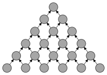
(a) Empty pyramid.

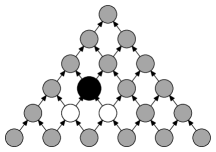
(b) Introduction move.

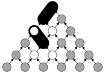
(c) Two subconfigurations before merger.

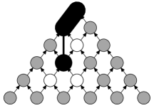
(d) The merged subconfiguration.

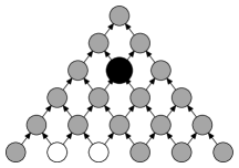
(e) Subconfiguration before inflation.

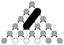
(f) Subconfiguration after inflation.

Figure 5. Examples of moves in the blob-pebble game.

Definition 4.8 (Blob-pebble game [BN08]).

If $B$ and $W$ are sets of vertices with $B\neq\emptyset$, $B\,\cap\,W=\emptyset$, we say that $[{B}]\langle{W}\rangle$ is a blob subconfiguration with a black blob on $B$ and white pebbles on $W$ supporting $B$. A blob-pebbling of a DAG $G$ with unique sink $z$ is a sequence $\mathcal{P}=\bigl{\{}\mathbb{P}_{0},\ldots,\mathbb{P}_{\tau}\bigr{\}}$ of blob subconfiguration sets, or blob-pebbling configurations, such that $\mathbb{P}_{0}=\emptyset$, $\mathbb{P}_{\tau}=\{[{z}]\langle{\emptyset}\rangle\}$, and for all $t\in[{\tau}]$, $\mathbb{P}_{t}$ is obtained from $\mathbb{P}_{t-1}$ by one of the following rules:

1. Introduction: $\mathbb{P}_{t}=\mathbb{P}_{t-1}\,\cup\,\{[{v}]\langle{\mathit{pred}(v)}\rangle\}$.

2. Merger: $\mathbb{P}_{t}=\mathbb{P}_{t-1}\,\cup\,\bigl{\{}[{B_{1}\,\cup\,B_{2}}]\langle{W_{1}\,\cup\,W_{2}}\rangle\bigr{\}}$ if there are $[{B_{1}}]\langle{W_{1}\,\cup\,\{v\}}\rangle,[{B_{2}\,\cup\,\{v\}}]\langle{W_{2}}\rangle\in\mathbb{P}_{t-1}$ such that $B_{1}\,\cap\,W_{2}=\emptyset$.

3. Inflation: $\mathbb{P}_{t}=\mathbb{P}_{t-1}\,\cup\,\bigl{\{}[{B\,\cup\,B^{\prime}}]\langle{W\,\cup\,W^{\prime}}\rangle\bigr{\}}$ if $[{B}]\langle{W}\rangle\in\mathbb{P}_{t-1}$ and $(B\,\cup\,B^{\prime})\,\cap\,\mbox{$(W\,\cup\,W^{\prime})$}=\emptyset$.

4. Erasure: $\mathbb{P}_{t}=\mathbb{P}_{t-1}\setminus\bigl{\{}[{B}]\langle{W}\rangle\bigr{\}}$ for $[{B}]\langle{W}\rangle\in\mathbb{P}_{t-1}$.

Let us now return to the proof outline in Section 3.1. The first step in our approach is to establish that any resolution refutation of a pebbling contradiction can be interpreted as a pebbling (but now in our modified game) of the DAG in terms of which this pebbling contradiction is defined. Intuitively, axiom downloads in the refutation will be matched by introduction moves in the blob-pebbling, erasures correspond to erasures, and seemingly suboptimal derivation steps can be modelled by inflation moves in the blob-pebbling. In all three papers [Nor09a, NH13, BN08], the formal definitions are set up so that a theorem along the following lines can be proven.

Tentative Theorem .

Consider a pebbling contradiction ${\mathit{Peb}_{G}}[{f}]$ over any DAG $G$. Then there is a translation function from sets of clauses over $\mathit{Vars}\bigl{(}{{\mathit{Peb}_{G}}[{f}]}\bigr{)}$ to sets of black blobs and white pebbles in $G$ that translates any resolution refutation $\pi$ of ${\mathit{Peb}_{G}}[{f}]$ into a blob-pebbling $\mathcal{P}_{\pi}$ of $G$.

The next step is to show pebbling lower bounds. Since the rules in the blob-pebble game are different from those of the standard black-white pebble game, known bounds on black-white pebbling price in the literature no longer apply. But again, provided that we have got the right definitions in place, we hope to be able to establish that the blob-pebblings can do no better than standard black-white pebblings.

Tentative Theorem .

If there is a blob-pebbling of a DAG $G$ in time $\tau$ and space $s$, then there is a standard black-white pebbling of $G$ in time $\mathrm{O}(\tau)$ and space $\mathrm{O}(s)$.

Finally, we need to establish that the number of pebbles used in $\mathcal{P}_{\pi}$ in Tentative Theorem 4.2 is related to the space of the resolution refutation $\pi$. As we know from Section 3.1, such a bound cannot be true for formulas $\mathit{Peb}_{G}$ so this is where we need to do substitutions with some suitable Boolean function $f_{d}$ over $d\geq 2$ variables and study ${\mathit{Peb}_{G}}[{f_{d}}]$.

Tentative Theorem .

If $\pi$ is a resolution refutation of a pebbling contradiction ${\mathit{Peb}_{G}}[{f_{d}}]$ for some suitable Boolean function $f_{d}$, then the time and space of the associated blob-pebbling $\mathcal{P}_{\pi}$ of $G$ are upper bounded by $\pi$ by $\text{{{time}}}(\mathcal{P}_{\pi})=\mathrm{O}(\mathit{L}(\pi))$ and $\text{{{space}}}(\mathcal{P}_{\pi})=\mathrm{O}(\mathit{Sp}(\pi))$.

If we put these three theorems together, it is clear that we can translate pebbling trade-offs to resolution trade-offs as described in the “theorem template” at the end of Section 3.1.

There is a catch, however, which is why we have used the label “tentative theorems” above. It is reasonably straightforward to come up with natural definitions that allow us to prove Tentative Theorem 4.2. But this in itself does not yield any lower bounds. (Indeed, there is a natural translation from refutations to pebbling even for $\mathit{Peb}_{G}$, for which we know that the lower bounds we are after do not hold!) The lower bounds instead follow from the combination of Tentative Theorems 4.2 and 4.2, but there is a tension between these two theorems.

The attentive reader might already have noted that two crucial details in Definition 4.8 are missing—we have not defined pebbling time and space for blob-pebblings. And for a good reason, because this turns out to be where the difficulty lies. On the one hand, we want the time and space measures for blob-pebblings to be as strong as possible, so that we can make Tentative Theorem 4.2 hold, saying that blob-pebblings can do no better than standard pebblings. On the other hand, we do not want the definitions to be too strong, for if so the bounds we need in Tentative Theorem 4.2 might break down. This turns out to be the major technical difficulty in the construction

In the papers [Nor09a, NH13], which study formulas ${\mathit{Peb}_{G}}[{\lor_{2}}]$ defined in terms of binary logical or, we cannot make any connection between pebbling time and refutation length in Tentative Theorems 4.2 and 4.2, but instead have to focus on only clause space. Also, the constructions work not for general DAGs but only for binary trees in [Nor09a], and only for a somewhat more general class of graphs also including pyramids in [NH13]. The reason for this is that it is hard to charge for black blobs and white pebbles. If we could charge for all vertices covered by blobs and pebbles, or at least one space unit for every black blob and every white pebble, we would be in good shape. But it appears hard to do so without losing the connection to clause space that we want in Tentative Theorem 4.2. Instead, for formulas ${\mathit{Peb}_{G}}[{\lor_{2}}]$ the best space measure that we can come up with is as follows.

Definition 4.9 (Blob-pebbling price with respect to $\lor_{2}$).

Let $\mathbb{P}={\{[{B_{i}}]\langle{W_{i}}\rangle\mid i=1,\ldots,n\}}$ be a set of blob subconfigurations over some DAG $G$.

A chargeable black blob collection of $\mathbb{P}$ is an ordered subset $\{B_{1},\ldots,B_{m}\}$ of black blobs in $\mathbb{P}$ such that for all $i\leq m$ it holds that $B_{i}\setminus\bigcup_{j<i}B_{j}\neq\emptyset$ (i.e., the unions $\bigcup_{j<i}B_{j}$ are strictly expanding for $i=1,\ldots,m$). We say that such a collection has black cost $m$.

The set of chargeable white pebbles of a subconfiguration $[{B_{i}}]\langle{W_{i}}\rangle\in\mathbb{P}$ is the subset of vertices $w\in W_{i}$ that are below all $b\in B_{i}$ (where “below” means that there is a path from $w$ to $b$ in $G$). The chargeable white pebble collection of $\mathbb{P}$ is the union of all such vertices for all $[{B_{i}}]\langle{W_{i}}\rangle\in\mathbb{P}$, and the white cost is the size of this set.

The space of a blob-pebbling configuration $\mathbb{P}$ is the largest black cost of a chargeable blob collection plus the cost of the chargeable white pebble collection, and the space of a blob-pebbling is the maximal space of any blob-pebbling configuration in it. The blob-pebbling price $\text{{{Blob-Peb}}}(G)$ of a DAG $G$ is the minimum space of any complete blob-pebbling of $G$.

Using the translation of clauses to blobs and pebbles in [BN08] it can be verified that Tentative Theorem 4.2 as proven in that paper holds also for formulas ${\mathit{Peb}_{G}}[{\lor_{2}}]$. Moreover, extending the proof techniques in [Nor09a, NH13] it is also not too hard to show the space bound in Tentative Theorem 4.2. But we do not know how to establish the space part in Tentative Theorem 4.2 for general DAGs. This is the part of the construction where [Nor09a] works only for binary trees and [NH13] can be made to work also for pyramids but not for general graphs.

The crucial new idea added in [BN08] to make the approach outlined above work for general DAGs was to switch formulas from ${\mathit{Peb}_{G}}[{\lor_{2}}]$ to ${\mathit{Peb}_{G}}[{f}]$ for other functions $f$ such as for instance binary exclusive or $\oplus_{2}$. However, while this does make the analysis much simpler (and stronger), it is not at all clear that the change of formulas should be necessary. We find it an intriguing question whether the program in Tentative Theorems 4.2, 4.2, and 4.2 could in fact be carried out for formulas $\mathit{Peb}_{G}[{\lor_{2}}]$.

[[Nor12]] Is it true for any DAG $G$ that any resolution refutation $\pi$ of $\mathit{Peb}_{G}[{\lor_{2}}]$ can be translated into a black-white pebbling of $G$ with time and space upper-bounded in terms of the length and space of $\pi$?

In particular, can we translate upper bounds in the blob-pebble game in Definition 4.8 with space defined as in Definition 4.9 to upper bounds for standard black-white pebbling? (From which clause space lower bounds for $\mathit{Peb}_{G}[{\lor_{2}}]$ would immediately follow.)

Our take on the results in [Nor09a, NH13] is that they can be interpreted as indicating that this should indeed be the case. Although, as noted above, these results apply only to limited classes of graphs, and only capture space lower bounds and not time-space trade-offs, the problems arising in the analysis seem to have to do more with artifacts in the proofs than with any fundamental differences between formulas $\mathit{Peb}_{G}[{\lor_{2}}]$ and, say, $\mathit{Peb}_{G}[{\oplus_{2}}]$. We remark that the papers [BN08, BN11] do not shed any light on this question, as the techniques used there inherently cannot work for formulas defined in terms of (non-exclusive) logical or.

If Open Problem 4.9 could be resolved in the positive, this could potentially be useful for settling the complexity of decision problems for resolution proof space, i.e., the problem given a CNF formula ${F}$ and a space bound $s$ to determine whether ${F}$ has a resolution refutation in space at most $s$. Reducing from pebbling space by way of formulas $\mathit{Peb}_{G}[{\lor_{2}}]$ would avoid the blow-up of the gap between upper and lower bounds on pebbling space that cause problems when using, for instance, exclusive or.

But let us return to the paper [BN08] that resolves the problems identified in [Nor09a, NH13]. The reason that we gain from switching from formulas ${\mathit{Peb}_{G}}[{\lor_{2}}]$ to, for instance, formulas ${\mathit{Peb}_{G}}[{\oplus_{2}}]$ is that for the latter formulas we can define a much stronger space measure for the blob-pebblings. In this case, it turns out that one can in fact charge for all vertices covered by blobs or pebbles in the blob-pebble game, and then the space bound in Tentative Theorem 4.2 follows for arbitrary DAGs. In the follow-up work [BN11] this result was improved to capture not only space but also the connection between pebbling time and refutation length, thus realizing the full program described in Section 3.1.

In this process, [BN11] also presented a much cleaner way to argue more generally about how the refutation length and space of a CNF formula ${F}$ change when we do substitution with some Boolean function $f$ to obtain ${{F}}[{f}]$. Since we believe that this is an interesting result in its own right, we give an exposition of it in Section 5. Before doing so, we want to conclude the current discussion by giving some examples from [BN08, BN11] of the kind of results obtained by these techniques.

4.3. Statement of Space Lower Bounds and Length-Space Trade-offs

Regarding the question of the relationship between length and space in resolution, [BN08] showed that in contrast to the tight relation between length versus width, length and space are as uncorrelated as they can possibly be.

Theorem 4.10 (Length-space separation for resolution [BN08]).

There exist explicitly constructible families of $k$-CNF formulas $\{{F}_{n}\}_{n=1}^{\infty}$ of size $\Theta(n)$ that can be refuted in resolution in length $\mathrm{O}(n)$ and width $\mathrm{O}(1)$ simultaneously, but for which any resolution refutation must have clause space $\Omega(n/\log n)$.

An extension of this theorem to $k$-DNF resolution in [BN11] showed that this family of proof systems does indeed form a strict hierarchy with respect to space.

Theorem 4.11 ($k$-DNF resolution space hierarchy [BN11]).

For every $k\geq 1$ there exists an explicitly constructible family $\{{F}_{n}\}_{n=1}^{\infty}$ of CNF formulas of size $\Theta(n)$ and width $\mathrm{O}(1)$ such that there are $\mathcal{R}({k+1})$-refutations ${{\pi_{n}}:{{F}_{n}}\,{\vdash}\,{\bot}}$ in simultaneous length $\mathit{L}(\pi_{n})=\mathrm{O}(n)$ and formula space $\mathit{Sp}(\pi_{n})=\mathrm{O}(1)$, but any $\mathcal{R}({k})$-refutation of ${F}_{n}$ requires formula space $\Omega\bigl{(}\sqrt[k+1]{n/\log n}\bigr{)}$. The constants hidden by the asymptotic notation depend only on $k$.

The formula families $\{{F}_{n}\}_{n=1}^{\infty}$ in Theorems 4.10 and 4.11 are obtained by considering pebbling contradictions over the graphs examined in Section LABEL:sec:optimal-lower-bound requiring black-white pebbling space $\Theta(n/\log n)$, and substituting a $k$-non-authoritarian Boolean function $f$ of arity $k+1$, for instance XOR over $k+1$ variables, in these formulas.

The above theorems give absolute lower bounds on space for resolution and $\mathcal{R}({k})$. Applying the techniques in [BN11] we can also derive length-space trade-offs for these proof systems. In fact, we can obtain a multitude of such trade-offs, since for any graph family with tight dual trade-offs for black and black-white pebbling, or for which black-white pebblings can be cast in the framework of Section 4.1 and simulated by resolution, we can obtain a corresponding trade-off for resolution-based proof systems. Since a full catalogue listing all of these trade-off results would be completely unreadable, we try to focus on some of the more salient examples below.

From the point of view of space complexity, the easiest formulas are those refutable in constant total space, i.e., formulas having so simple a structure that there are resolution refutations where we never need to keep more than a constant number of symbols on the proof blackboard. A priori, it is not even clear whether we should expect that any trade-off phenomena could occur for such formulas, but it turns out that there are quadratic length-space trade-offs.

Theorem 4.12 (Quadratic trade-offs for constant space [BN11]).

For any fixed positive integer $K$ there are explicitly constructible CNF formulas $\{{F}_{n}\}_{n=1}^{\infty}$ of size $\Theta(n)$ and width $\mathrm{O}(1)$ such that the following holds (where all multiplicative constants hidden in the asymptotic notation depend only on $K$): $\bullet$

The formulas ${F}_{n}$ are refutable in syntactic resolution in total space $\mbox{${\mathit{TotSp}}_{\mathcal{R}}({F}_{n}\vdash\!\bot)$}\!=\!\mathrm{O}(1)$.

For any monotone function $s_{\mathrm{hi}}(n)=\mathrm{O}\bigl{(}\sqrt{n}\bigr{)}$ there are syntactic resolution refutations $\pi_{n}$ of ${F}_{n}$ in simultaneous length $\mathit{L}(\pi_{n})=\mathrm{O}\bigl{(}(n/s_{\mathrm{hi}}(n))^{2}\bigr{)}$ and total space $\mathit{TotSp}(\pi_{n})=\mathrm{O}(s_{\mathrm{hi}}(n))$.

For any semantic resolution refutation ${{\pi_{n}}:{{F}_{n}}\,{\vdash}\,{\bot}}$ in clause space $\mathit{Sp}(\pi_{n})\leq s_{\mathrm{hi}}(n)$ it holds that $\mathit{L}(\pi_{n})=\Omega\bigl{(}(n/s_{\mathrm{hi}}(n))^{2}\bigr{)}$.

For any $k\leq K$, any semantic $k$-DNF resolution refutation $\pi_{n}$ of ${F}_{n}$ in formula space $\mathit{Sp}(\pi_{n})\leq s_{\mathrm{hi}}(n)$ must have length $\mathit{L}(\pi_{n})=\Omega\left(\bigl{(}n/s_{\mathrm{hi}}(n)^{k+1}\bigr{)}^{2}\right)$. In particular, any semantic constant-space $\mathcal{R}({k})$-refutation must also have quadratic length.

Theorem 4.12 follows by combining the techniques to be discussed in Section 5 with the pebbling trade-offs in Section LABEL:sec:constant-space-trade-offs and the structural results on simulations of black-white pebblings by resolution in Theorem 4.5.

Remark 4.13.

Notice that the trade-off applies to both formula space—i.e., clause space for $\mathcal{R}({1})$—and total space. This is because the upper bound is stated in terms of the larger of these two measures (total space) while the lower bound is in terms of the smaller one (formula space). Note also that the upper bounds hold for the usual, syntactic versions of the proof systems, whereas the lower bounds hold for the much stronger semantic systems, and that for standard resolution the upper and lower bounds are tight up to constant factors. These properties hold for all trade-offs stated below. Finally, we remark that we have to pick some arbitrary but fixed limit $K$ for the size of the terms when stating the results for $k$-DNF resolution, since for any family of formulas we consider there will be very length- and space-efficient $\mathcal{R}({k})$-refutation refutations if we allow terms of unbounded size.

Our next example is based on the pebbling trade-off result in Section LABEL:sec:non-constant-space-trade-offs. Using this new result, we can derive among other things the rather striking statement that for any arbitrarily slowly growing non-constant function, there are explicit formulas of such (arbitrarily small) space complexity that nevertheless exhibit superpolynomial length-space trade-offs.

Theorem 4.14 (Superpolynomial trade-offs for arbitrarily slowly growing space [BN11]).

Let $s_{\mathrm{lo}}(n)=\omega(1)$ be any arbitrarily slowly growing function and fix any $\epsilon>0$ and positive integer $K$. Then there are explicitly constructible CNF formulas $\{{F}_{n}\}_{n=1}^{\infty}$ of size $\Theta(n)$ and width $\mathrm{O}(1)$ such that the following holds: $\bullet$

The formulas ${F}_{n}$ are refutable in syntactic resolution in total space $\mbox{${\mathit{TotSp}}_{\mathcal{R}}({F}_{n}\vdash\!\bot)$}\!=\!\mathrm{O}(s_{\mathrm{lo}}(n))$.

There are syntactic resolution refutations $\pi_{n}$ of ${F}_{n}$ in simultaneous length $\mathit{L}(\pi_{n})=\mathrm{O}(n)$ and total space $\mathit{TotSp}(\pi_{n})=\mathrm{O}\left(\bigl{(}n/s_{\mathrm{lo}}(n)^{2}\bigr{)}^{1/3}\right)$.

Any semantic resolution refutation of ${F}_{n}$ in clause space $\mathrm{O}\left(\bigl{(}n/s_{\mathrm{lo}}(n)^{2}\bigr{)}^{1/3-\epsilon}\right)$ must have superpolynomial length.

For any $k\leq K$, any semantic $\mathcal{R}({k})$-refutation of ${F}_{n}$ in formula space $\mathrm{O}\left(\bigl{(}n/s_{\mathrm{lo}}(n)^{2}\bigr{)}^{1/(3(k+1))-\epsilon}\right)$ must have superpolynomial length. All multiplicative constants hidden in the asymptotic notation depend only on $K$, $\epsilon$ and $s_{\mathrm{lo}}$.

Observe the robust nature of this trade-off, which is displayed by the long range of space complexity in standard resolution, from $\omega(1)$ up to $\approx n^{1/3}$, which requires superpolynomial length. Note also that the trade-off result for standard resolution is very nearly tight in the sense that the superpolynomial lower bound on length in terms of space reaches up to very close to where the linear upper bound kicks in.

The two theorems above focus on trade-offs for formulas of low space complexity, and the lower bounds on length obtained in the trade-offs are somewhat weak—the superpolynomial growth in Theorem 4.14 is something like $n^{s_{\mathrm{lo}}(n)}$. We next present a theorem that has both a stronger superpolynomial length lower bounds than Theorem 4.14 and an even more robust trade-off covering a wider (although non-overlapping) space interval. This theorem again follows by applying our tools to the pebbling trade-offs in Section LABEL:sec:robust-trade-offs established by [LT82].

Theorem 4.15 (Robust superpolynomial trade-off for medium-range space [BN11]).

For any positive integer $K$, there are explicitly constructible CNF formulas $\{{F}_{n}\}_{n=1}^{\infty}$ of size $\Theta(n)$ and width $\mathrm{O}(1)$ such that the following holds (where the hidden constants depend only on $K$): $\bullet$

The formulas ${F}_{n}$ are refutable in syntactic resolution in total space $\mbox{${\mathit{TotSp}}_{\mathcal{R}}({F}_{n}\vdash\!\bot)$}\!=\!\mathrm{O}(\log^{2}n)$.

There are syntactic resolution refutations of ${F}_{n}$ in length $\mathrm{O}(n)$ and total space $\mathrm{O}(n/\log n)$.

Any semantic resolution refutation of ${F}_{n}$ in clause space $\mathit{Sp}(\pi_{n})=\mathrm{o}(n/\log n)$ must have length $\mathit{L}(\pi_{n})=n^{\Omega(\log\log n)}$.

For any $k\leq K$, any semantic $k$-DNF resolution refutation of ${F}_{n}$ in formula space $\mathit{Sp}(\pi_{n})=\mathrm{o}\left((n/\log n)^{1/(k+1)}\right)$ must have length $\mathit{L}(\pi_{n})=n^{\Omega(\log\log n)}$.

Having presented trade-off results in the low-space and medium-space range, we conclude by presenting a result at the other end of the space spectrum. Namely, appealing one last time to yet another result in [LT82], this time from Section LABEL:sec:exponential-trade-offs, we can deduce that there are formulas of nearly linear space complexity (recall that any formula is refutable in linear formula space) that exhibit not only superpolynomial but even exponential trade-offs.

We state this final theorem for standard resolution only since it is not clear whether it makes sense for $\mathcal{R}({k})$. That is, we can certainly derive formal trade-off bounds in terms of the $(k+1)$st square root as in the theorems above, but we do not know whether there actually exist $\mathcal{R}({k})$-refutation in sufficiently small space so that the trade-offs apply. Hence, such trade-off claims for $\mathcal{R}({k})$, although impressive-looking, might simply be vacuous. It is possible to obtain other exponential trade-offs for $\mathcal{R}({k})$ but they are not quite as strong as the result below for resolution. We refer to [BN11] for the details.

Theorem 4.16 (Exponential trade-offs for nearly-linear space [BN11]).

Let $\kappa$ be any sufficiently large constant. Then there are CNF formulas ${F}_{n}$ of size $\Theta(n)$ and width $\mathrm{O}(1)$ and a constant $\kappa^{\prime}\ll\kappa$ such that: $\bullet$

The formulas ${F}_{n}$ have syntactic resolution refutations in total space $\kappa^{\prime}\cdot n/\log n$.

${F}_{n}$ is also refutable in syntactic resolution in length $\mathrm{O}(n)$ and total space $\mathrm{O}(n)$ simultaneously.

However, any semantic refutation of ${F}_{n}$ in clause space at most $\kappa\cdot n/\log n$ has length $\exp\bigl{(}n^{\Omega(1)}\bigr{)}$.

To get a feeling for this last trade-off result, note again that the lower bound holds for proof systems with arbitrarily strong derivation rules, as long as they operate with disjunctive clauses. In particular, it holds for proof systems that can in one step derive anything that is semantically implied by the current content of the blackboard. Recall that such a proof system can refute any unsatisfiable CNF formula ${F}$ with $n$ clauses in length $n+1$ simply by writing down all clauses of ${F}$ on the blackboard and then concluding, in one single derivation step, the contradictory empty clause implied by ${F}$. In Theorem 4.16 the semantic resolution proof system has space nearly sufficient for such an ultra-short refutation of the whole formula. But even so, when we feed this proof system the formulas ${F}_{n}$ and restrict it to having at most $\mathrm{O}(n/\log n)$ clauses on the blackboard at any one given time, it will have to keep going for an exponential number of steps before it is finished.

5. Deriving Time-Space Trade-offs via the Substitution Theorem

A paradigm that has turned out to be useful in many contexts in proof complexity is to take a CNF formula family $\{{F}_{n}\}_{n=1}^{\infty}$ with interesting properties, tweak it by substituting some function $f(x_{1},\ldots,x_{d})$ for each variable $x$, and then use this new formula family to prove the desired result. Although this approach often is not made explicit in the respective papers, most of the results reviewed in Sections 3 and 4 can be viewed as applying variations on this theme to pebbling formulas.

Another example of this approach is the observation by Alekhnovich and Razborov, referenced (and used) in [Ben09, BP07], that if we take a CNF formula ${F}$ and apply substitution with binary exclusive or $\oplus_{2}$, then the length of refuting the substituted formula ${{F}}[{\oplus_{2}}]$ in resolution is exponential in the refutation width of the original formula, i.e., ${\mathit{L}}({{F}}[{\oplus_{2}}]\vdash\!\bot)=\exp\bigl{(}\Omega({\mathit{W}}({F}\vdash\!\bot))\bigr{)}$. The proof is by applying a random restriction to the variables of ${{F}}[{\oplus_{2}}]$ by picking one variable $x_{i}$ from each pair $x_{1},x_{2}$ and setting this variable to a random value. This restriction gives us back the original formula ${F}$ (possibly after flipping polarity of literals), and also eliminates all wide clauses in a refutation with high probability. Since restrictions preserve resolution refutations, we can conclude that if there is no narrow refutation of ${F}$, then there cannot be a short refutation of ${{F}}[{\oplus_{2}}]$.

If we take a closer look at the space lower bounds and length-space trade-offs for substituted pebbling contradictions in Section 4.3, it turns out that the only fact we need about the pebbling formulas is that they have linear-length proofs in small width but that there is a weak trade-off between length and variable space. The rest of the argument can be seen to be totally oblivious to the fact that we are dealing with pebbling formulas. The only property we use for these formulas is the trade-off between length and variable space, and that substitution with the right function $f$ can be used to lift these trade-offs to length versus the much stronger measure clause space.

In this section, we want to give a clean exposition of how substitution in CNF formulas can be used to amplify length-space trade-offs for resolution-based proof systems. We believe that these results are interesting in their own right, and that they can potentially open the way for similar results for even stronger proof systems.

5.1. Preserving Upper Bounds for Substituted Formulas

If we want to use substitution to prove tight trade-offs, we need to show that the substituted formulas become harder but not too hard, since we want to be able to establish matching upper bounds. It is straightforward to show that if ${F}$ is easy for resolution, then any substitution formula ${{F}}[{f}]$ is also easy in the following sense.

Lemma 5.1 ([BN11]).

Suppose that ${F}$ is an unsatisfiable CNF formula and that $f:\{0,1\}^{d}\to\{0,1\}$ is a non-constant Boolean function. If there is a resolution refutation $\pi$ of ${F}$ in length $\mathit{L}(\pi)={\mathit{L}}$, clause space $\mathit{Sp}(\pi)=s$, and width $\mathit{W}(\pi)=w$, then there is also a resolution refutation $\pi_{f}$ of ${{F}}[{f}]$ in length $\mathit{L}\bigl{(}\pi_{f}\bigr{)}={\mathit{L}}\cdot\exp(\mathrm{O}(dw))$, clause space $\mathit{Sp}\bigl{(}\pi_{f}\bigr{)}=s\cdot\exp(\mathrm{O}(dw))$, and width $\mathit{W}\bigl{(}\pi_{f}\bigr{)}=\mathrm{O}(dw)$.

In particular, if the refutation ${{\pi}:{{F}}\,{\vdash}\,{\bot}}$ has constant width, then it is possible to refute ${{F}}[{f}]$ with only a constant factor blow-up in length and space as compared to $\pi$ (where this constant depends on $\mathit{W}(\pi)$ and $f$). Of course, the same holds for any sequential proof system $\mathcal{P}$ that can simulate resolution proofs efficiently line by line, such as, for instance, cutting planes or polynomial calculus resolution.

The upper bounds for ${{F}}[{f}]$ in Lemma 5.1 are not hard to show. Briefly, the proof is as follows. Given a resolution refutation $\pi$ of ${F}$, we construct a refutation ${{\pi_{f}}:{{{F}}[{f}]}\,{\vdash}\,{\bot}}$ mimicking the derivation steps in $\pi$. When $\pi$ downloads an axiom $C$, we download all the axiom clauses in ${C}[{f}]$, which is a set of at most $\exp\bigl{(}\mathrm{O}(d\cdot\mathit{W}(C))\bigr{)}$ clauses. When $\pi$ resolves $C_{1}\lor x$ and $C_{2}\lor\overline{x}$ to derive $C_{1}\lor C_{2}$, we use the fact that resolution is implicationally complete to derive ${(C_{1}\lor C_{2})}[{f}]$ from ${(C_{1}\lor x)}[{f}]$ and ${(C_{2}\lor\overline{x})}[{f}]$ in at most $\exp\bigl{(}\mathrm{O}(d\cdot\mathit{W}(C_{1}\lor C_{2}))\bigl{)}$ steps. When a clause $C$ is erased in $\pi$, we erase all clauses ${C}[{f}]$ in $\pi_{f}$. We refer to [BN11] for the formal details.

A more interesting question is under which circumstances moderate hardness results for ${F}$ can be amplified to stronger hardness results for ${{F}}[{f}]$. In what follows, we will describe a general framework in which weak space lower bounds and length-space trade-offs for resolution can be lifted to strong lower bounds and trade-offs for resolution or even more powerful proof systems. This framework is just a straightforward generalization and unification of what was done in [BN11], but we believe that the more general language below helps us to uncover the essence of the argument and makes it easier to see the potential for (as well as the problems with) strengthening the results in [BN11] even further.

5.2. Projections

The idea behind our approach is as follows: Start with a CNF formula ${F}$ which has some nice properties for resolution. Consider now some proof system $\mathcal{P}$ (which might be resolution, or some other, stronger system) and study the substitution formula ${{F}}[{f}]$, where we have chosen $f$ to have the right properties with respect to $\mathcal{P}$. Let $\pi_{f}$ be any $\mathcal{P}$-refutation of ${{F}}[{f}]$. Intuitively, we want to argue that the best thing $\mathcal{P}$ can do is to mimic a resolution refutation $\pi$ of ${F}$ as described in the proof sketch for Lemma 5.1 above. We then observe that in such simulations of resolution refutations of ${F}$, the weak lower bounds for ${F}$ are blown up to strong lower bounds for ${{F}}[{f}]$.

Formally speaking, we cannot really hope to prove this, since it is hard to place restrictions on what $\mathcal{P}$ might or might not do when refuting ${{F}}[{f}]$. However, what we can do is to argue that whatever a $\mathcal{P}$-refutation $\pi_{f}$ of ${{F}}[{f}]$ looks like, we can extract from this $\pi_{f}$ a resolution refutation $\pi$ of ${F}$. Our way of doing this is to define projections of arbitrary Boolean function over $\mathit{Vars}^{d}({V})$ to clauses over $V$, and to show that such projections translate $\mathcal{P}$-refutations to resolution refutations.

Roughly, our intuition for projections is that if, for instance, a $\mathcal{P}$-configuration $\mathbb{D}$ implies $f(\vec{x})\lor\lnot f(\vec{y})$, then this should project the clause $x\lor\overline{y}$. It will be useful for us, however, to relax this requirement a bit and allow other definitions of projections as well as long as they are “in the same spirit.” We specify next which formal properties a projection must satisfy for our approach to work. For this definition, it will be convenient to have a compact notation for evaluating either $f$ or the complement of $f$. Extending our notation for literals, where $x^{1}=x$ and $x^{0}=\lnot x$, we define $f^{1}({\vec{x}})=f(\vec{x})$ and $f^{0}({\vec{x}})=\lnot f(\vec{x})$. Also for compactness, in what follows below we will sometimes write $x^{\nu}\in C$ instead of $x^{\nu}\in\mathit{Lit}({C})$ for a literal $x^{\nu}$ occuring in a clause $C$.

Definition 5.2 (Semantic projection).

Let $f:\{0,1\}^{d}\to\{0,1\}$ be a fixed Boolean function. Let $\mathcal{P}$ be a sequential proof system, and let $\mathbb{D}$ denote arbitrary sets of Boolean functions over $\mathit{Vars}^{d}({V})$ of the form specified by $\mathcal{P}$. Let $\mathbb{C}$ denote arbitrary sets of disjunctive clauses over $V$. Then the function ${\mathit{proj}\!}_{f}$ mapping set of Boolean functions $\mathbb{D}$ to clauses $\mathbb{C}$ is a semantic ${f}$-projection, or in what follows just an ${f}$-projection for short, if it is:

1. Complete: If $\mathbb{D}\vDash\bigvee_{x^{\nu}\in C}f^{\nu}({\vec{x}})$ then the clause $C$ either is in ${\mathit{proj}\!}_{f}({\mathbb{D}})$ or is derivable from ${\mathit{proj}\!}_{f}({\mathbb{D}})$ by weakening.

2. Nontrivial: If $\mathbb{D}=\emptyset$, then ${\mathit{proj}\!}_{f}({\mathbb{D}})=\emptyset$.

3. Monotone: If $\mathbb{D}^{\prime}\vDash\mathbb{D}$ and $C\in{\mathit{proj}\!}_{f}({\mathbb{D}})$, then either $C\in{\mathit{proj}\!}_{f}({\mathbb{D}^{\prime}})$ or $C$ is derivable from ${\mathit{proj}\!}_{f}({\mathbb{D}^{\prime}})$ by weakening.

4. Incrementally sound: Let $A$ be a clause over $V$ and let $L_{A}$ be the encoding of some clause in ${A}[{f}]$ as a Boolean function of the type prescribed by $\mathcal{P}$. Then if $C\in{\mathit{proj}\!}_{f}({\mathbb{D}\,\cup\,\{L_{A}\}})$, it holds for all literals $a\in\mathit{Lit}({A})\setminus\mathit{Lit}({C})$ that the clause $\overline{a}\lor C$ either is in ${\mathit{proj}\!}_{f}({\mathbb{D}})$ or can be derived from ${\mathit{proj}\!}_{f}({\mathbb{D}})$ by weakening.

In what follows, for conciseness we will use the phrase that some clause $C$ “can be derived from ${\mathit{proj}\!}_{f}({\mathbb{D}})$ by weakening” to mean that there is some clause $C^{\prime}\subseteq C$ such that $C^{\prime}\in{\mathit{proj}\!}_{f}({\mathbb{D}})$, i.e., to cover both cases that $C\in{\mathit{proj}\!}_{f}({\mathbb{D}})$ or that the clause is derivable by weakening of some other clause in ${\mathit{proj}\!}_{f}({\mathbb{D}})$.

A special kind of projections are those that look not only on all of $\mathbb{D}$ “globally,” but measure the semantic content of $\mathbb{D}$ more precisely.

Definition 5.3 (Local projection).

If ${\mathit{proj}\!}_{f}$ is an ${f}$-projection, then its localized version ${\mathit{proj}\!}^{\,L}_{f}$ is defined to be ${\mathit{proj}\!}^{\,L}_{f}({\mathbb{D}})=\bigcup_{\mathbb{D}^{\prime}\subseteq\mathbb{D}}{\mathit{proj}\!}_{f}({\mathbb{D}^{\prime}})$. If ${\mathit{proj}\!}_{f}={\mathit{proj}\!}^{\,L}_{f}$, we say that ${\mathit{proj}\!}_{f}$ is a local projection.

It is easily verified that the localized version of a projection is indeed itself a projection in the sense of Definition 5.2.

In order for our approach outlined above to work, the most important property of a projection is that it should somehow preserve space when going from the proof system $\mathcal{P}$ to resolution.

Definition 5.4 (Space-faithful projection).

Consider a sequential proof system $\mathcal{P}$ with space measure $\mathit{Sp}(\cdot)$. Let $f:\{0,1\}^{d}\to\{0,1\}$ be a fixed Boolean function, and suppose that ${\mathit{proj}\!}_{f}$ is an ${f}$-projection. Then we say that ${\mathit{proj}\!}_{f}$ is space-faithful of degree $K$ with respect to $\mathcal{P}$ if there is a polynomial $Q$ of degree at most $K$ such that for any set of Boolean functions $\mathbb{D}$ over $\mathit{Vars}^{d}({V})$ on the form prescribed by $\mathcal{P}$, it holds that $Q(\mathit{Sp}(\mathbb{D}))\geq\bigl{\lvert}\mathit{Vars}({{\mathit{proj}\!}_{f}({\mathbb{D}})})\bigr{\rvert}$. We say that ${\mathit{proj}\!}_{f}$ is linearly space-faithful if $Q$ has degree $1$, and that ${\mathit{proj}\!}_{f}$ is exactly space-faithful if we can choose $Q(x)=x$.

The way Definition 5.4 should be understood is that the smaller the degree, the tighter the reduction between the proof system $\mathcal{P}$ and resolution will be.

5.3. The Substitution Theorem and Trade-off Lower Bounds

We now show that if we can design a projection in accordance with Definition 5.2, then this projection can be used to extract resolution refutations from refutations in sequential implicational proof systems $\mathcal{P}$ (as defined at the beginning of Section 2.2). Furthermore, if our projection is space-faithful, this extraction operation will preserve length-space trade-off (with some loss in parameters depending on how high the degree $K$ is).

Lemma 5.5.

Let $\mathcal{P}$ be a sequential implicational proof system and let $f:\{0,1\}^{d}\to\{0,1\}$ be a Boolean function, and suppose that ${\mathit{proj}\!}_{f}$ is an ${f}$-projection. Then for any CNF formula ${F}$ it holds that if $\pi_{f}=\{\mathbb{D}_{0},\mathbb{D}_{1},\ldots,\mathbb{D}_{\tau}\}$ is a semantic $\mathcal{P}$-refutation of the substitution formula ${{F}}[{f}]$, the sequence of sets of projected clauses $\bigl{\{}{\mathit{proj}\!}_{f}({\mathbb{D}_{0}}),{\mathit{proj}\!}_{f}({\mathbb{D}_{1}}),\ldots,{\mathit{proj}\!}_{f}({\mathbb{D}_{\tau}})\bigr{\}}$ forms the “backbone” of a resolution refutation $\pi$ of ${F}$ in the following sense:

1. ${\mathit{proj}\!}_{f}({\mathbb{D}_{0}})=\emptyset$.

2. $\bot\in{\mathit{proj}\!}_{f}({\mathbb{D}_{\tau}})$.

3. All transitions from ${\mathit{proj}\!}_{f}({\mathbb{D}_{t-1}})$ to ${\mathit{proj}\!}_{f}({\mathbb{D}_{t}})$ for $t\in[{\tau}]$ can be accomplished in syntactic resolution in such a fashion that $\mathit{VarSp}(\pi)=\mathrm{O}\bigl{(}\max_{\mathbb{D}\in\pi_{f}}\{\mathit{VarSp}({\mathit{proj}\!}_{f}({\mathbb{D}}))\}\bigr{)}$, or, if ${\mathit{proj}\!}_{f}$ is a local projection, so that $\mathit{VarSp}(\pi)\leq\max_{\mathbb{D}\in\pi_{f}}\{\mathit{VarSp}({\mathit{proj}\!}_{f}({\mathbb{D}}))\}$.

4. The length of $\pi$ is upper-bounded by $\pi_{f}$ in the sense that the only time $\pi$ performs a download of an axiom $C\in{F}$ is when $\pi_{f}$ downloads some axiom $D\in{C}[{f}]$ from ${{F}}[{f}]$.

On the one hand, Lemma 5.5 is very strong in the sense that even semantic $\mathcal{P}$-refutations can be translated to syntactic resolution refutations. On the other hand, it would have been nice if the bound in part 4 of Lemma 5.5 could have been made into a true upper bound in terms of the length of $\pi_{f}$, but it is easy to see that this is not possible. The reason for this is precisely that the $\mathcal{P}$-proof refuting ${{F}}[{f}]$ is allowed to use any arbitrarily strong semantic inference rules, and this can lead to exponential savings compared to syntactic resolution. For a concrete example, just let ${F}$ be an encoding of the pigeonhole principle and let $\pi_{f}$ be the refutation that downloads all axioms of ${{F}}[{f}]$ and then derives contradiction in one step. An interesting question is whether it would be possible to circumvent this problem by modifying Definition 5.2 to some kind of “syntactic” projection instead, but we do not know if and how this can be done. Also, it is not clear that it would help much—for the applications we have in mind the bound in terms of axiom downloads is enough, and allows us to obtain stronger bounds that hold not only for syntactic but even semantic $\mathcal{P}$-proofs.

Before proving Lemma 5.5 let us see how it can be used to prove trade-offs provided that we can construct space-faithful projections.

Theorem 5.6.

Let $\mathcal{P}$ be a sequential proof system with space measure $\mathit{Sp}(\cdot)$. Suppose $f:\{0,1\}^{d}\to\{0,1\}$ is a Boolean function such that there exists an ${f}$-projection which is space-faithful of degree $K$ with respect to $\mathcal{P}$. Then if ${F}$ is any unsatisfiable CNF formula and $\pi_{f}$ is any semantic $\mathcal{P}$-refutation of the substitution formula ${{F}}[{f}]$, there is a resolution refutation $\pi$ of ${F}$ such that: $\bullet$

The length of $\pi$ is upper-bounded by $\pi_{f}$ in the sense that $\pi$ makes at most as many axiom downloads as $\pi_{f}$.

The space of $\pi$ is upper-bounded by $\pi_{f}$ in the sense that $\mathit{VarSp}(\pi)=\mathrm{O}\bigl{(}\mathit{Sp}(\pi_{f})^{K}\bigr{)}$.

In particular, if there is no syntactic resolution refutation of ${F}$ in variable space $\mathrm{O}(s)$ making $\mathrm{O}({\mathit{L}})$ axiom downloads, then there is no semantic $\mathcal{P}$-refutation of ${{F}}[{f}]$ in simultaneous length $\mathrm{O}({\mathit{L}})$ and $\mathcal{P}$-space $\mathrm{O}\bigl{(}\sqrt[K]{s}\bigr{)}$.

Proof 5.7 (Proof of Theorem 5.6).

Let $\pi_{f}$ be a semantic $\mathcal{P}$-refutation of ${{F}}[{f}]$, and let $\pi$ be the resolution refutation we obtain by applying the the projection ${\mathit{proj}\!}_{f}$ on $\pi_{f}$ as in Lemma 5.5. By part 4 of Lemma 5.5 we know that $\pi$ makes at most as many axiom downloads as $\pi_{f}$. By part 3 of the lemma we have $\mathit{VarSp}(\pi)=\mathrm{O}\bigl{(}\max_{\mathbb{D}\in\pi_{f}}\{\mathit{VarSp}({\mathit{proj}\!}_{f}({\mathbb{D}}))\}\bigr{)}$. Fix some $\mathcal{P}$-configuration $\mathbb{D}$ maximizing the right-hand side of this expression. For this $\mathbb{D}$ we have $\mathit{VarSp}({\mathit{proj}\!}_{f}({\mathbb{D}}))=\mathrm{O}\bigl{(}\mathit{Sp}(\mathbb{D})^{K}\bigr{)}=\mathrm{O}\bigl{(}\mathit{Sp}(\pi_{f})^{K}\bigr{)}$ according to Definition 5.4. The theorem follows.

Clearly, the key to the proof of Theorem 5.6 is the claim that projections translate $\mathcal{P}$-refutations to resolution refutations. Let us substantiate this claim.

Proof 5.8 (Proof of Lemma 5.5).

Fix any sequential proof system $\mathcal{P}$, any ${f}$-projection ${\mathit{proj}\!}_{f}$, and any CNF formula ${F}$. Recall that we want to show that if $\pi_{f}=\{\mathbb{D}_{0},\mathbb{D}_{1},\ldots,\mathbb{D}_{\tau}\}$ is a semantic $\mathcal{P}$-refutation of the substitution formula ${{F}}[{f}]$, then the sequence of projected clause sets $\bigl{\{}{\mathit{proj}\!}_{f}({\mathbb{D}_{0}}),{\mathit{proj}\!}_{f}({\mathbb{D}_{1}}),\ldots,{\mathit{proj}\!}_{f}({\mathbb{D}_{\tau}})\bigr{\}}$ is essentially a resolution refutation $\pi$ except for some details that we might have to fill in when going from ${\mathit{proj}\!}_{f}({\mathbb{D}_{t-1}})$ to ${\mathit{proj}\!}_{f}({\mathbb{D}_{t}})$ in the derivation.

Parts 1 and 2 of Lemma 5.5 are immediate from Definition 5.2, since we have ${\mathit{proj}\!}_{f}({\mathbb{D}_{0}})={\mathit{proj}\!}_{f}({\emptyset})=\emptyset$ by nontriviality and $\bot\in{\mathit{proj}\!}_{f}({\mathbb{D}_{\tau}})$ by completeness (note that $\mathbb{D}_{\tau}\vDash\bot=\bigvee_{x^{\nu}\in\bot}f^{\nu}({\vec{x}})$ and the empty clause clearly cannot be derived by weakening).

We want to show that a resolution refutation of ${F}$ can get from ${\mathit{proj}\!}_{f}({\mathbb{D}_{t-1}})$ to ${\mathit{proj}\!}_{f}({\mathbb{D}_{t}})$ as claimed in part 3 of the lemma. For brevity, let us write $\mathbb{C}_{i}={\mathit{proj}\!}_{f}({\mathbb{D}_{i}})$ for all $i$, and consider the possible derivation steps at time $t$.

Inference

Suppose $\mathbb{D}_{t}=\mathbb{D}_{t-1}\,\cup\,\{L_{t}\}$ for some $L_{t}$ inferred from $\mathbb{D}_{t-1}$. Since $\mathcal{P}$ is sound we have $\mathbb{D}_{t-1}\vDash\mathbb{D}_{t}$, and since the projection is monotone by definition we can conclude that all clauses in $\mathbb{C}_{t}\setminus\mathbb{C}_{t-1}$ are derivable from $\mathbb{C}_{t-1}$ by weakening. We go from $\mathbb{C}_{t-1}$ to $\mathbb{C}_{t}$ in three steps. First, we erase all clauses $C\in\mathbb{C}_{t-1}$ for which there are no clauses $C^{\prime}\in\mathbb{C}_{t}$ such that $C\subseteq C^{\prime}$. Then, we derive all clauses in $\mathbb{C}_{t}\setminus\mathbb{C}_{t-1}$ by weakening, noting that all clauses needed for weakening steps are still in the configuration. Finally, we erase the rest of $\mathbb{C}_{t}\setminus\mathbb{C}_{t-1}$. At all times during this transition from $\mathbb{C}_{t-1}$ to $\mathbb{C}_{t-1}$, the variable space of the intermediate clause configurations is upper-bounded by $\max\{\mathit{VarSp}(\mathbb{C}_{t-1}),\mathit{VarSp}(\mathbb{C}_{t})\}$.

Erasure

Suppose $\mathbb{D}_{t}=\mathbb{D}_{t-1}\setminus\{L_{t-1}\}$ for some $L_{t-1}\in\mathbb{D}_{t-1}$. Again we have that $\mathbb{D}_{t-1}\vDash\mathbb{D}_{t}$, and we can appeal to the monotonicity of the projection and proceed exactly as in the case of an inference above.

Axiom download

So far, the only derivation rules used in the resolution refutation $\pi$ that we are constructing are weakening and erasure, which clearly does not help $\pi$ to make much progress towards proving a contradiction. Also, the only properties of the ${f}$-projection that we have used are completeness, nontriviality, and monotonicity. Note, however, that a “projection” that sends $\emptyset$ to $\emptyset$ and all other configurations to $\{\bot\}$ also satisfies these conditions. Hence, the axiom downloads are where we must expect the action to take place, and we can also expect that we will have to make crucial use of the incremental soundness of the projection.

Assume that $\mathbb{D}_{t}=\mathbb{D}_{t-1}\,\cup\,\{L_{A}\}$ for a function $L_{A}$ encoding some clause from the substitution clause set ${A}[{f}]$ corresponding to an axiom $A\in{F}$. We want to show that all clauses in $\mathbb{C}_{t}\setminus\mathbb{C}_{t-1}$ can be derived in $\pi$ by downloading $A$, resolving (and possibly weakening) clauses, and then perhaps erasing $A$, and that all this can be done without the variable space exceeding $\mathit{VarSp}(\mathbb{C}_{t-1}\,\cup\,\mathbb{C}_{t})\leq\mathit{VarSp}(\mathbb{C}_{t-1})+\mathit{VarSp}(\mathbb{C}_{t})$.

We already know how to derive clauses by weakening, so consider a clause $C\in\mathbb{C}_{t}\setminus\mathbb{C}_{t-1}$ that cannot be derived by weakening from $\mathbb{C}_{t-1}$. By the incremental soundness of the projection, it holds for all literals $a\in\mathit{Lit}({A})\setminus\mathit{Lit}({C})$ that the clauses $\overline{a}\lor C$ can be derived from $\mathbb{C}_{t-1}$ by weakening. Once we have these clauses, we can resolve them one by one with $A$ to derive $C$.

Some care is needed, though, to argue that we can stay within the variable space bound $\mathit{VarSp}(\mathbb{C}_{t-1})+\mathit{VarSp}(\mathbb{C}_{t})$. Observe that what was just said implies that for all $a\in\mathit{Lit}({A})\setminus\mathit{Lit}({C})$ there are clauses $\overline{a}\lor C_{a}\in\mathbb{C}_{t-1}$ with $C_{a}\subseteq C$. In particular, we have $\overline{a}\in\mathit{Lit}({\mathbb{C}_{t-1}})$ for all $a\in\mathit{Lit}({A})\setminus\mathit{Lit}({C})$. This is so since by the incremental soundness there must exist some clause $C^{\prime}\in\mathbb{C}_{t-1}$ such that $\overline{a}\lor C$ is derivable by weakening from $C^{\prime}$, and if $\overline{a}\notin\mathit{Lit}({C^{\prime}})$ we would have that $C$ is derivable by weakening from $C^{\prime}$ as well, contrary to assumption. Note furthermore that if the projection is local, then $\overline{a}\lor C_{a}\in\mathbb{C}_{t-1}$ implies that $\overline{a}\lor C_{a}\in\mathbb{C}_{t}$ as well, since no clauses can disappear from the projection when enlarging $\mathbb{D}_{t-1}$ to $\mathbb{D}_{t}$. Thus, for local projections we have $\mathit{VarSp}(\mathbb{C}_{t-1}\,\cup\,\{A\})\subseteq\mathit{VarSp}(\mathbb{C}_{t})$.

If it happens that all clauses in $\mathbb{C}_{t}\setminus\mathbb{C}_{t-1}$ can be derived by weakening, we act as in the cases of inference and erasure above. Otherwise, to make the transition from $\mathbb{C}_{t-1}$ to $\mathbb{C}_{t}$ in a space-efficient fashion we proceed as follows.

1. Download the axiom clause $A$.

2. Infer all clauses in $\mathbb{C}_{t}\setminus\mathbb{C}_{t-1}$ that can be derived by weakening from $\mathbb{C}_{t-1}\,\cup\,\{A\}$.

3. For all remaining clauses $C\in\mathbb{C}_{t}\setminus\mathbb{C}_{t-1}$, derive $\overline{a}\lor C$ for all literals $a\in\mathit{Lit}({A})\setminus\mathit{Lit}({C})$ and then resolve these clauses with $A$ to obtain $C$.

4. Erase all clauses in the current configuration that are not present in $\mathbb{C}_{t}$, possibly including $A$.

Since it follows from what was argued above that $\mathit{Vars}({A})\subseteq\mathit{Vars}({\mathbb{C}_{t-1}\,\cup\,\mathbb{C}_{t}})$, all the variables in all the intermediate configurations above will be contained in this set, meaning that the variable space never exceeds $\mathit{VarSp}(\mathbb{C}_{t-1})+\mathit{VarSp}(\mathbb{C}_{t})$. If in addition the projection is local, then $\mathit{VarSp}(\mathbb{C}_{t-1}\,\cup\,\{A\})\subseteq\mathit{VarSp}(\mathbb{C}_{t})$ and the variable space increases monotonically from $\mathbb{C}_{t-1}$ to $\mathbb{C}_{t}$.

Wrapping up the proof, we have shown that no matter what $\mathcal{P}$-derivation step is made in the transition $\mathbb{D}_{t-1}\rightsquigarrow\mathbb{D}_{t}$, it is possible to perform the corresponding transition $\mathbb{C}_{t-1}\rightsquigarrow\mathbb{C}_{t}$ for our projected clause sets in resolution without the variable space going above $\mathit{VarSp}(\mathbb{C}_{t-1})+\mathit{VarSp}(\mathbb{C}_{t})$ (or even above $\mathit{VarSp}(\mathbb{C}_{t})$ for local projections). Also, the only time we need to download an axiom $A\in{F}$ in our projected refutation $\pi$ of ${F}$ is when $\pi_{f}$ downloads some axiom from ${A}[{f_{d}}]$. The lemma follows.

5.4. Resolution and $k$-DNF Resolution Have Space-Faithful Projections

Let us recall again what Theorem 5.6 says. Suppose we have a family of CNF formulas with lower bounds for refutation variable space in resolution, or with trade-offs between refutation length and refutation variable space (such as for instance pebbling contradictions over suitable graphs). Then we can lift these lower bounds and trade-offs to stronger measures in a potentially stronger proof system $\mathcal{P}$, provided that we can find a Boolean function $f:\{0,1\}^{d}\to\{0,1\}$ and an ${f}$-projection ${\mathit{proj}\!}_{f}$ that is space-faithful with respect to $\mathcal{P}$.

Thus, at this point we can in principle forget everything about proof complexity. If we want to prove space lower bounds or time-space trade-offs for a proof system $\mathcal{P}$, we can focus on studying Boolean functions of the form used by $\mathcal{P}$ and trying to devise space-faithful projections for such functions. Below, we describe how this can be done for resolution and $\mathcal{R}({k})$-systems.

Definition 5.9 (Precise implication [BN11]).

Let $f$ be a Boolean function of arity $d$, let $\mathbb{D}$ be a set of Boolean functions over $\mathit{Vars}^{d}({V})$, and let $C$ be a disjunctive clause over $V$. If

$$\mathbb{D} \vDash\bigvee_{x^{\nu}\in C}f^{\nu}({\vec{x}})$$ (12a)

but for all strict subclauses $$C^{\prime}\subsetneqq C$$ it holds that

$$\mathbb{D} \nvDash\bigvee_{x^{\nu}\in C^{\prime}}f^{\nu}({\vec{x}})\enspace,$$ (12b)

we say that the clause set $\mathbb{D}$ implies $\bigvee_{x^{\nu}\in C}f^{\nu}({\vec{x}})$ precisely and write

$$\mathbb{D}\vartriangleright\bigvee_{x^{\nu}\in C}f^{\nu}({\vec{x}})\enspace.$$ (13)

Definition 5.10 (Resolution projection).

Let $f$ denote a Boolean function of arity $d$ and let $\mathbb{D}$ be any set of Boolean functions over $\mathit{Vars}^{d}({V})$. Then we define

$${\mathit{Rproj}\!}_{f}({\mathbb{D}})={\{C\mid\mathbb{D}\vartriangleright\bigvee_{x^{\nu}\in C}f^{\nu}({\vec{x}})\}}$$ (14)

to be the resolution projection of $\mathbb{D}$. Also, we define ${\mathit{Rproj}\!}^{\,L}_{f}({\mathbb{D}})=\bigcup_{\mathbb{D}^{\prime}\subseteq\mathbb{D}}{\mathit{Rproj}\!}_{f}({\mathbb{D}^{\prime}})$ to be the local resolution projection of $\mathbb{D}$.

Lemma 5.11.

The mapping ${\mathit{Rproj}\!}_{f}$ is an ${f}$-projection (for any sequential proof system $\mathcal{P}$).

Proof 5.12.

Suppose $\mathbb{D}\vDash\bigvee_{x^{\nu}\in C}f^{\nu}({\vec{x}})$. Then we can remove literals from $C$ one by one until we have some minimal clause $C^{\prime}\subseteq C$ such that no more literal can be removed if the implication is to hold, and this clause $C^{\prime}$ is projected by $\mathbb{D}$ according to the definition. This proves both completeness and monotonicity for ${\mathit{Rproj}\!}_{f}$. Nontriviality is obvious.

For the incremental soundness, if $C\in{\mathit{Rproj}\!}_{f}({\mathbb{D}\,\cup\,\{L_{A}\}})$ for an encoding $L_{A}$ of some clause in ${A}[{f}]$, then this means, in particular, that $\mathbb{D}\,\cup\,\{L_{A}\}\vDash\bigvee_{x^{\nu}\in C}f^{\nu}({\vec{x}})$. Consider any truth value assignment ${\alpha}$ such that ${\alpha}(\mathbb{D})=1$ but ${\alpha}\bigl{(}\bigvee_{x^{\nu}\in C}f^{\nu}({\vec{x}})\bigr{)}=0$. By assumption, ${\alpha}(L_{A})=0$. But this means that for all literals $y^{\mu}\in\mathit{Lit}({A})$ we have ${\alpha}\bigl{(}f^{1-\mu}({\vec{y}})\bigr{)}=1$. Since this holds for any ${\alpha}$, it follows for all $y^{\mu}\in\mathit{Lit}({A})$ that $\mathbb{D}\vDash\bigvee_{x^{\nu}\in(y^{1-\mu}\lor C)}f^{\nu}({\vec{x}})$, and we conclude by the completeness of the projection that the clause $y^{1-\mu}\lor C$ is derivable by weakening from ${\mathit{Rproj}\!}_{f}({\mathbb{D}})$.

With this projection, and using Theorem 5.6, the main technical result in [BN11] can now be rephrased as follows, where we recall the notion of non-authoritarian functions from Definition 2.12.

Theorem 5.13 ([BN11]).

If $f$ is a non-authoritarian Boolean function, then the projection ${\mathit{Rproj}\!}^{\,L}_{f}$ is exactly space-faithful with respect to the resolution proof system.

This result was later extended to $k$-DNF resolution, although with slightly worse parameters.

Theorem 5.14 ([BN11]).

If $f$ is a $(k+1)$-non-authoritarian function (for some fixed $k$), then the projection ${\mathit{Rproj}\!}_{f}$ is space-faithful of degree $k+1$ with respect to $k$-DNF resolution.

It has subsequently been shown that the loss in the parameters in Theorem 5.14 as compared to Theorem 5.13 is necessary, except perhaps for an additive constant $1$ in the degree.

Theorem 5.15 ([NR11]).

If $f$ is the exclusive or of $k+1$ variables, then the projection ${\mathit{Rproj}\!}_{f}$ cannot be space-faithful with respect to $k$-DNF resolution for any degree $K<k$.

As an aside, it can be noted that Theorem 5.13 uses the local version of the projection, whereas Theorem 5.14 uses the non-local definition. Theorem 5.13 can be made to work with either variant (if we are willing to settle for a projection that is just linearly space-faithful instead of exactly space-faithful), but for technical reasons the proof of Theorem 5.14 only seems to work with the “global” version of the projection.

Although this might not be immediately obvious, Theorems 5.13 and 5.14 are remarkably powerful tools for understanding space in resolution-based proof systems. All the trade-off lower bounds in Section 4 can be derived as immediate consequences of these two theorems. Another interesting corollary of Theorem 5.13 is that that it yields optimal lower bounds on clause space for resolution. Recall that Esteban and Torán [ET01] proved that the clause space of refuting ${F}$ is upper-bounded by the formula size. In the papers [ABRW02, BG03, ET01] it was shown, using quite elaborate arguments, that there are polynomial-size $k$-CNF formulas with lower bounds on clause space matching this upper bound up to constant factors. Using Theorem 5.13 we can get a different and much shorter proof of this fact.

Corollary 5.16 ([ABRW02, BG03, ET01]).

There are families of $k$-CNF formulas $\{{F}\}_{n=1}^{\infty}$ with $\Theta(n)$ clauses over $\Theta(n)$ variables such that ${\mathit{Sp}}_{\mathcal{R}}({F}_{n}\vdash\!\bot)=\Theta(n)$.

Proof 5.17.

Just pick any formula family for which it is shown that any refutation of ${F}_{n}$ must at some point in the refutation mention $\Omega(n)$ variables at the same time (for example, from [BW01]), and then apply Theorem 5.13 to, say, ${{F}_{n}}[{\oplus_{2}}]$.

It should be noted, though, that to derive these linear lower bounds we have to change the formula families by substitution, whereas the papers [ABRW02, BG03, ET01] prove their lower bounds for the original formulas. Moreover, there is another, and even more elegant way to derive Corollary 5.16 from [BW01] without having to modify the formulas under consideration, namely by using the lower bound on clause space in terms of width in [AD08].

As we indicated above, we believe that this projection framework can potentially be extended to other proof systems than resolution and $\mathcal{R}({k})$. In particular, it would be very interesting to see if one could prove lower bounds for cutting planes, polynomial calculus, or polynomial calculus resolution in this way. However, to do so another projection (in the sense of Definition 5.2) than the one in Definition 5.10 would be needed. We conclude this section by sketching the proofs of Theorems 5.13 and 5.14, and then explaining why the same approach will not work for CP, PC, or PCR.

Proof 5.18 (Proof sketch for Theorem 5.13).

In the case of resolution, the set of Boolean functions $\mathbb{D}$ just consists of disjunctive clauses over $\mathit{Vars}^{d}({V})$. Fix some clause set $\mathbb{D}$ and let $V^{*}=\mathit{Vars}\bigl{(}{{\mathit{Rproj}\!}^{\,L}_{f}({\mathbb{D}})}\bigr{)}$. What we want to prove is that $\lvert\mathbb{D}\rvert\geq\lvert V^{*}\rvert$.

To this end, consider the bipartite graph with the vertices on the left labelled by clauses $D\in\mathbb{D}$ and the vertices on the right labelled by variables $x\in V^{*}$. We draw an edge between $D$ and $x$ if some variable $x_{i}$ belonging to $x$ appears in $D$. Let $N(\mathbb{D}^{\prime})$ denote the neighbours on the right of a clause set $\mathbb{D}^{\prime}$. We claim without proof that $N(\mathbb{D})=V^{*}$, i.e., that all $x\in V^{*}$ have incoming edges from $\mathbb{D}$ (this follows from the condition (12b) in Definition 5.9).

Pick some $\mathbb{D}_{1}\subseteq\mathbb{D}$ of maximal size (possibly empty) with a set of neighbours $V^{*}_{1}=N(\mathbb{D}_{1})$ such that $\lvert\mathbb{D}_{1}\rvert\geq\lvert V^{*}_{1}\rvert$. If $\mathbb{D}_{1}=\mathbb{D}$ we are done, so let us suppose $\mathbb{D}_{1}\neq\mathbb{D}$ and argue by contradiction. Let $\mathbb{D}_{2}=\mathbb{D}\setminus\mathbb{D}_{1}\neq\emptyset$ and $V^{*}_{2}=V^{*}\setminus V^{*}_{1}$. For all $\mathbb{D}^{\prime}\subseteq\mathbb{D}_{2}$ we must have $\lvert\mathbb{D}^{\prime}\rvert\leq\lvert N(\mathbb{D}^{\prime})\setminus V^{*}_{1}\rvert=\lvert N(\mathbb{D}^{\prime})\,\cap\,V^{*}_{2}\rvert$, since otherwise $\mathbb{D}_{1}$ would not have been chosen of maximal size. This in turns implies by Hall’s theorem that there is a matching $M$ from $\mathbb{D}_{2}$ into $V^{*}_{2}$.

Consider some clause $C\in{\mathit{Rproj}\!}^{\,L}_{f}({\mathbb{D}})$ such that $\mathbb{D}_{1}$ is “too weak” to project $C$ (we are fudging some details here again, but nothing important). Let $C_{i}$ be the part of $C$ that mentions variables from $V^{*}_{i}$ for $i=1,2$. Then by Definitions 5.9 and 5.10 it holds that $\mathbb{D}_{1}\,\cup\,\mathbb{D}_{2}\vDash\bigvee_{x^{\nu}\in C_{1}}f^{\nu}({\vec{x}})\,\lor\,\bigvee_{y^{\nu}\in C_{2}}f^{\nu}({\vec{y}})$ but $\mathbb{D}_{1}\nvDash\bigvee_{x^{\nu}\in C_{1}}f^{\nu}({\vec{x}})$. This means that there is a truth value assignment ${\alpha}_{1}$ to $\mathit{Vars}^{d}({V^{*}_{1}})$ satisfying $\mathbb{D}_{1}$ but falsifying $\bigvee_{x^{\nu}\in C_{1}}f^{\nu}({\vec{x}})$. Observe that $\mathit{Vars}({\mathbb{D}_{1}})\subseteq\mathit{Vars}^{d}({V^{*}_{1}})$ by construction.

Using the matching $M$, we can find another partial truth value assignment ${\alpha}_{2}$ to $\mathit{Vars}^{d}({V^{*}_{2}})$ that satisfies $\mathbb{D}_{2}$ by setting at most one variable $x_{i}$ for every $x\in V^{*}_{2}$. This ${\alpha}_{2}$ leaves the truth value of $\bigvee_{y^{\nu}\in C_{2}}f^{\nu}({\vec{y}})$ undetermined since $f$ is non-authoritarian, and this means that we can extend ${\alpha}_{2}$ to a full assignment over $\mathit{Vars}^{d}({V^{*}_{2}})$ such that $\bigvee_{y^{\nu}\in C_{2}}f^{\nu}({\vec{y}})$ is falsified. But then ${\alpha}_{1}\,\cup\,{\alpha}_{2}$ is an assignment that satisfies $\mathbb{D}_{1}\,\cup\,\mathbb{D}_{2}$ but falsifies $\bigvee_{x^{\nu}\in C_{1}}f^{\nu}({\vec{x}})\,\lor\,\bigvee_{y^{\nu}\in C_{2}}f^{\nu}({\vec{y}})$, which is a contradiction.

Proof 5.19 (Proof sketch for Theorem 5.14 ).

Let us restrict our attention to $2$-DNF resolution, since this already captures the hardness of the general case. Also, we sweep quite a few technical details under the rug to focus on the main idea of the proof.

Suppose that we have a set of $2$-DNF formulas $\mathbb{D}$ of size $\lvert\mathbb{D}\rvert=m$ such that the set of projected variables $V^{*}=\mathit{Vars}({{\mathit{Rproj}\!}_{f}({\mathbb{D}})})$ has size $\lvert V^{*}\rvert\geq K\cdot m^{3}$ for some suitably large constant $K$ of our choice. We want to derive a contradiction.

As a first preprocessing step, let us prune all formulas $D\in\mathbb{D}$ one by one by shrinking any $2$-term $a\land b$ in $D$ to just $a$ or just $b$, i.e., making $D$ weaker, as long as this does not change the projection ${\mathit{Rproj}\!}_{f}({\mathbb{D}})$. This pruning step does not decrease the size (i.e., the number of formulas) of $\mathbb{D}$.

By counting, there must exist some formula $D\in\mathbb{D}$ containing literals belonging to at least $K\cdot m^{2}$ different variables in $V^{*}$. Consider some clause $C\in{\mathit{Rproj}\!}_{f}({\mathbb{D}})$ such that $\mathbb{D}\setminus\{D\}$ is too weak to project it. This means that there is an assignment ${\alpha}$ such that ${\alpha}(\mathbb{D}\setminus\{D\})=1$ but ${\alpha}\bigl{(}\bigvee_{x^{\nu}\in C}f^{\nu}({\vec{x}})\bigr{)}\neq 1$, i.e., ${\alpha}$ either fixes ${\alpha}\bigl{(}\bigvee_{x^{\nu}\in C}f^{\nu}({\vec{x}})\bigr{)}$ to false or leaves it undetermined. Let us pick such an ${\alpha}$ assigning values to the minimal amount of variables. It is clear that the domain size of ${\alpha}$ will then be at most $2(m-1)$ since the assignment needs to fix only one $2$-term for every formula in $\mathbb{D}\setminus\{D\}$. But this means that the formula $D$ contains a huge number of unset variables. We would like to argue that somewhere in $D$ there is a $2$-term that can be set to true without satisfying $\bigvee_{x^{\nu}\in C}f^{\nu}({\vec{x}})$, which would lead to a contradiction.

We note first that if $D$ contains $2m$ $2$-terms $x^{\nu}_{i}\land y^{\mu}_{j}$ with all literals in these terms belonging to pairwise disjoint variable sets for distinct terms (but where we can have $x=y$), we immediately get a contradiction. Namely, if this is the case we can find at least one $2$-term $x^{\nu}_{i}\land y^{\mu}_{j}$ such that ${\alpha}$ does not assign values to any variables $x_{i^{\prime}},y_{j^{\prime}}$. We can satisfy this $2$-term, and hence all of $\mathbb{D}$, without satisfying $\bigvee_{x^{\nu}\in C}f^{\nu}({\vec{x}})$ since by assumption $f$ is $3$-non-authoritarian (so any assignments to $x_{i}$ and $y_{j}$ can be repaired by setting other variables $x_{i^{\prime}},y_{j^{\prime}}$ to appropriate values).

But if $D$ does not contain $2m$ such $2$-terms over disjoint variables, then by counting (and adjusting our constant $K$) there must exist some literal $a$ that occurs in $D$ in at least $2m$ terms $a\land x^{\nu}_{i}$ with the $x_{i}$ belonging to different variables. Moreover, these $2$-terms were not pruned in our preprocessing step, so they must all be necessary. Because of this, one can argue that there must exist some other assignment ${\alpha}^{\prime}$ such that ${\alpha}^{\prime}(\mathbb{D}\setminus\{D\})=1$, ${\alpha}^{\prime}\bigl{(}\bigvee_{x^{\nu}\in C}f^{\nu}({\vec{x}})\bigr{)}\neq 1$, and ${\alpha}^{\prime}(a)=1$. Now at least one of the $2m$ companion variables of $a$ is untouched by ${\alpha}^{\prime}$ and can be set to true without satisfying $\bigvee_{x^{\nu}\in C}f^{\nu}({\vec{x}})$. This is a contradiction.

To see why we cannot hope to prove lower bounds for cutting planes or polynomial calculus in the same fashion, consider the following examples.

Example 5.20.

If we have variables $x[1],x[2],x[3],\ldots$ and make substitutions using binary exclusive or $\oplus_{2}$ to get new variables $x[1]_{1},x[1]_{2},x[2]_{1},x[2]_{2},x[3]_{1},x[3]_{2},\ldots$, then the example

$$\sum_{i=1}^{k}(x[i]_{1}-x[i]_{2})\geq k$$ (15)

shows that just a single CP inequality can project an arbitrarily large conjunction $x[1]\land x[2]\land\cdots\land x[k]$. Thus, here we have $\lvert\mathbb{D}\rvert=1$ while $\mathit{VarSp}({\mathit{Rproj}\!}_{\oplus_{2}}({\mathbb{D}}))$ goes to infinity.

Example 5.21.

Again using substitutions with $\oplus_{2}$, for polynomial calculus we have the example

$$-1+\prod_{i=1}^{k}x[i]_{1}x[i]_{2}$$ (16)

showing that just two monomials can project the arbitrarily large conjunction $\overline{x[1]}\land\overline{x[2]}\land\cdots\land\overline{x[k]}$ if we use the projection in Definition 5.10.

Let us also give a slightly more involved example for polynomial calculus resolution that uses the extra formal variables encoding negative literals to obtain projected configurations with many positive literals. Recall that in PCR we write $x^{\prime}$ to denote the formal variable that encodes the negation of $x$.

Example 5.22.

In PCR, three monomials

$$-1+\prod_{i=1}^{k}x[i]_{1}x[i]_{2}^{\prime}+\prod_{i=1}^{k}x[i]_{1}^{\prime}x[i]_{2}$$ (17)

can project the arbitrarily large conjunction $x[1]\land x[2]\land\cdots\land x[k]$ if we use the projection in Definition 5.10.

Somehow, the reason that these counter-examples work is that the projection in Definition 5.10 allows the Boolean functions in the implication to be far too strong. These functions do not really imply just conjunctions of exclusive ors, but something much stronger in that they actually fix the variable assignments (to some particular assignment that happens to satisfy exclusive ors). Note that formulas ${{F}}[{\oplus_{2}}]$ do not speak about fixed variable assignments for, say, $x_{1}$ or $x_{2}$, but only about the value of $x_{1}\oplus x_{2}$. Intuitively, therefore, the only way we can know something more about $x_{1}$ and $x_{2}$ than the value of $x_{1}\oplus x_{2}$ is if the refutation has already derived contradiction and is now deriving all kinds of other interesting consequences from this. But before this happens, we would like to argue that any refutation must pass through a stage where all it can know about $x_{1}$ and $x_{2}$ is the value of $x_{1}\oplus x_{2}$ and nothing more. For this reason, we would like to find a more “fine-grained” definition of a projection that can capture only these weaker implications and discard too strong implications.

Is it possible to prove space lower bounds and/or trade-offs between proof length/size and space for cutting planes, polynomial calculus, or polynomial calculus resolution by designing smarter projections than in Definition 5.10 that are space-faithful for these proof systems?

6. Some Open Problems Regarding Space Bounds and Trade-offs

Despite the progress made during the last few years on understanding space in resolution and how it is related to other measures, there are quite a few natural questions that still have not been resolved.

Perhaps one of the main open questions is how complex a $k$-CNF formula ${F}$ can be with respect to total space. If ${F}$ has at most $n$ clauses or variables (which is the case if, in particular, ${F}$ has size $n$) we know from [ET01] that ${\mathit{Sp}}_{\mathcal{R}}({F}\vdash\!\bot)\leq n+\mathrm{O}(1)$. From this it immediately follows that ${\mathit{TotSp}}_{\mathcal{R}}({F}\vdash\!\bot)=\mathrm{O}\bigl{(}n^{2}\bigr{)}$. But is this upper bound tight?

[[ABRW02]] Are there $k$-CNF formula families $\{{F}_{n}\}_{n=1}^{\infty}$ of size $\Theta(n)$ such that ${\mathit{TotSp}}({F}_{n}\vdash\!\bot)=\Omega\bigl{(}n^{2}\bigr{)}$?

As a first step towards resolving this question, Alekhnovich et al.[ABRW02] posed the problem of finding $k$-CNF formulas over $n$ variables and of size polynomial in $n$ such that ${\mathit{TotSp}}({F}\vdash\!\bot)=\omega(n)$. (There is a lower bound ${\mathit{TotSp}}({F}\vdash\!\bot)=\Omega(n^{2})$ proven in [ABRW02], but it is for formulas of exponential size and linear width). Alekhnovich et al.also conjectured that the answer to Open Problem 6 is yes, and suggested so-called Tseitin formulas defined over $3$-regular expander graphs as candidates for formulas ${F}_{n}$ of size $n$ with ${\mathit{TotSp}}({F}_{n}\vdash\!\bot)=\Omega\bigl{(}n^{2}\bigr{)}$.

Another natural open question is to separate polynomial calculus resolution from just resolution with respect to space.

Are there $k$-CNF formula families $\{{F}_{n}\}_{n=1}^{\infty}$ such that ${\mathit{Sp}}_{\mathcal{R}}({F}_{n}\vdash\!\bot)=\omega\bigl{(}{\mathit{Sp}}_{\mathcal{PCR}}({F}_{n}\vdash\!\bot)\bigr{)}$?

The next two questions that we want to address concern upper bounds on resolution length in terms of clause space. We know from [AD08] that clause space is an upper bound for width, and width yields an upper bound on length simply by counting. However, it would be more satisfying to find a more direct argument that explains why clause space upper-bounds length. Focusing on constant clause space for concreteness, the problem can be formulated as follows.

For $k$-CNF formulas ${F}$ of size $n$, we know that ${\mathit{Sp}}({F}\vdash\!\bot)=\mathrm{O}(1)$ implies ${\mathit{L}}({F}\vdash\!\bot)=\mathrm{poly}(n)$. Is there a direct proof of this fact, not going via [AD08]?

If we could understand this problem better, we could perhaps also find out whether it is possible to derive stronger upper bounds on length in terms of space. Esteban and Torán ask the following question.

[[ET01]] Does it hold for $k$-CNF formulas ${F}$ that ${\mathit{Sp}}({F}\vdash\!\bot)=\mathrm{O}(\log n)$ implies ${\mathit{L}}({F}\vdash\!\bot)=\mathrm{poly}(n)$?

Turning to the relationship between width and length, recall that we know from [BW01] that short resolution refutations imply the existence of narrow refutations, and that in view of this an appealing proof search heuristic is to search exhaustively for refutations in minimal width. One serious drawback of this approach, however, is that there is no guarantee that the short and narrow refutations are the same one. On the contrary, the narrow refutation constructed in the proof in [BW01] is potentially exponentially longer than the short refutation that one starts with. However, we have no examples of formulas where the refutation in minimum width is actually known to be substantially longer than the minimum-length refutation. Therefore, it would be interesting to know whether this increase in length is necessary. That is, is there a formula family which exhibits a length-width trade-off in the sense that there are short refutations and narrow refutations, but all narrow refutations have a length blow-up (polynomial or superpolynomial)? Or is the exponential blow-up in [BW01] just an artifact of the proof?

[[NH13]] If ${F}$ is a $k$-CNF formula over $n$ variables refutable in length ${\mathit{L}}$, can one always find a refutation $\pi$ of ${F}$ in width $\mathit{W}(\pi)={\mathrm{O}\bigl{(}\sqrt{n\log{\mathit{L}}}\bigr{)}}$ with length no more than, say, $\mathit{L}(\pi)={\mathrm{O}({\mathit{L}})}$ or at most $\mathrm{poly}({\mathit{L}})$? Or is there a formula family which necessarily exhibits a length-width trade-off in the sense that there are short refutations and narrow refutations, but all narrow refutations have a length blow-up (polynomial or superpolynomial)?

As was mentioned above, for tree-like resolution Ben-Sasson [Ben09] showed that there are formulas ${F}_{n}$ refutable in linear length and also in constant width, but for which any refutation $\pi_{n}$ must have $\mathit{W}(\pi_{n})\cdot\log\mathit{L}(\pi_{n})=\Omega(n/\log n)$. This shows that the length blow-up in the proof of the tree-like length-width relationships in [BW01] is necessary. That is, transforming a short tree-like proof into a narrow proof might necessarily incur an exponential length blow-up. But tree-like resolution is very different from unrestricted resolution in that upper bounds on width do not imply upper bounds on length (as shown in [BW01] using $\mathit{Peb}_{G}[{\lor_{2}}]$-formulas), so it is not clear that the result for tree-like resolution provides any intuition for the general case.

A related question about trade-offs between length and width on a finer scale, raised by Albert Atserias and Marc Thurley, is as follows.

[[AT09]] For $w\geq 3$ arbitrary but fixed, is there family of unsatisfiable $3$-CNF formulas $\{{F}_{n}^{w}\}_{n=1}^{\infty}$ of size $\Theta(n)$ that have resolution refutations of width $w$ but cannot be refuted in length $\mathrm{O}\bigl{(}n^{w-c}\bigr{)}$ for some small positive constant $c$?

This question was prompted by the paper [AFT11], where it was shown for a fairly general theoretical model of DPLL solvers with clause learning that in this model contradictory formulas ${F}_{n}$ with ${\mathit{W}}({F}_{n}\vdash\!\bot)=w$ are likely to be proven unsatisfiable in time $n^{\mathrm{O}(w)}$. It is natural to ask how much room for improvement there is for this time bound. Since these algorithms are resolution-based, it would be nice if one could prove a lower bound saying that there are formulas ${F}_{n}$ with ${\mathit{W}}({F}_{n}\vdash\!\bot)=w$ that cannot be refuted by resolution in length $n^{\mathrm{o}(w)}$, or even $n^{w-\mathrm{O}(1)}$. As a step towards proving (or disproving) this, resolving special cases of Open Problem 6 for concrete instantiations of the parameters, say $w=10$ and $w-c=2$, would also be of interest.

For resolution clause space, we know that there can be very strong trade-offs with respect to length for space $s$ in the range $\omega(1)=s=\mathrm{o}(n/\log\log n)$, but we do not know what holds for space outside of this range. Consider first formulas refutable by proofs $\pi$ in constant space. When we run such a refutation through the proof in [AD08] and obtain another narrow, and thus short, refutation $\pi^{\prime}$ we do not have any information about the space complexity of this refutation. Is it possible to get a refutation in both short length and small space simultaneously?

[[NH13]] Suppose that ${\{{F}_{n}\}}_{n=1}^{\infty}$ is a family of polynomial-size $k$-CNF formulas with refutation clause space $\mbox{${\mathit{Sp}}({F}_{n}\vdash\!\bot)$}=\mathrm{O}(1)$. Does this imply that there are resolution refutations ${{\pi_{n}}:{{F}_{n}}\,{\vdash}\,{\bot}}$ simultaneously in length $\mathit{L}(\pi_{n})=\mathrm{poly}(n)$ and clause space $\mathit{Sp}(\pi_{n})=\mathrm{O}(1)$? Or can it be that restricting the clause space, we sometimes have to end up with really long refutations?

Note that if we instead look at the total space measure (that also counts the number of literals in each clause with repetitions), then the answer to the above question is that we can obtain refutations that are both short and space-efficient simultaneously, again by a simple counting argument. But for clause space such a counting argument does not seem to apply, and maybe strange things can happen. (They certainly can in the sense that as soon as we go to arbitrarily slowly growing non-constant space, there provably exist strong space-length trade-offs.) Of course, one would expect here that any insight regarding Open Problem 6 should have bearing on this question as well.

Consider now space complexity at the other end of the range. Note that all trade-offs for clause space proven so far are in the regime where the space $\mathit{Sp}(\pi)$ is less than the number of clauses $\lvert{F}\rvert$ in ${F}$. On the one hand, this is quite natural, since the size of the formula is an upper bound on the refutation clause space needed. On the other hand, it is not clear that this should rule out length-space trade-offs for linear or superlinear space, since the proof that any formula is refutable in linear space constructs a resolution refutation that has exponential length. Assume therefore that we have a CNF formula ${F}$ of size $n$ refutable in length ${\mathit{L}}({F}\vdash\!\bot)={\mathit{L}}$ for ${\mathit{L}}$ suitably large (say, ${\mathit{L}}=\mathrm{poly}(n)$ or ${\mathit{L}}=n^{\log n}$ or so). Suppose that we allow clause space more than the minimum $n+\mathrm{O}(1)$, but less than the trivial upper bound ${\mathit{L}}/\log{\mathit{L}}$. Can we then find a resolution refutation using at most that much space and achieving at most a polynomial increase in length compared to the minimum?

[[Ben07, NH08]] Let ${F}$ be any $k$-CNF formula with $\lvert{F}\rvert=n$ clauses. Suppose that ${\mathit{L}}({F}\vdash\!\bot)={\mathit{L}}=\mathrm{poly}(n)$. Does this imply that there is a resolution refutation ${{\pi}:{{F}}\,{\vdash}\,{\bot}}$ in clause space $\mathit{Sp}(\pi)=\mathrm{O}(n)$ and length $\mathit{L}(\pi)=\mathrm{poly}({\mathit{L}})$? Or are there formulas with trade-offs in the range space $\geq$ formula size?

Finally, a slightly curious aspect of the space lower bounds and length-space trade-offs surveyed above is that the results in [Nor09a, NH13] only work for $k$-CNF formulas of width $k\geq 4$, and in [BN08, BN11] we even have to choose $k\geq 6$ to find $k$-CNF formula families that optimally separate space and length and exhibit time-space trade-offs. We know from [ET01] that any $2$-CNF formula is refutable in constant clause space, but should there not be $3$-CNF formulas for which we could prove similar separations and trade-offs?

Given any CNF formula ${F}$, we can transform it to a $3$-CNF formula by rewriting every clause $C=a_{1}\lor\ldots\lor a_{m}$ in ${F}$ with $m>3$ as a conjunction of $3$-clauses

$$\overline{y}_{0}\,\land\,\bigwedge_{1\leq i\leq m}(y_{i-1}\lor a_{i}\lor\overline{y}_{i})\,\land\,y_{n},$$ (18)

for some new auxiliary variables $y_{0},y_{1},\ldots,y_{m}$ unique for this clause $C$. Let us write $\widetilde{{F}}$ to denote the $3$-CNF formula obtained from ${F}$ in this way. It is easy to see that $\widetilde{{F}}$ is unsatisfiable if and only if ${F}$ is unsatisfiable. Also, it is straightforward to verify that $\mbox{${\mathit{L}}\bigl{(}\widetilde{{F}}\vdash\!\bot\bigr{)}$}\leq{\mathit{L}}({F}\vdash\!\bot)+\mathrm{O}(\mathit{W}({F})\cdot\mathit{L}({F}))$ and ${\mathit{Sp}}\bigl{(}\widetilde{{F}}\vdash\!\bot\bigr{)}\leq{\mathit{Sp}}({F}\vdash\!\bot)+{\mathrm{O}\bigl{(}1\bigr{)}}$. (Just note that each clause of ${F}$ can be derived from $\widetilde{{F}}$ in length $2\cdot\mathit{W}({F})+3$ and space $3$, and then use this together with an optimal refutation of ${F}$.)

It seems like a natural idea to rewrite pebbling contradictions $\mathit{Peb}_{G}[{f}]$ for suitable functions $f$ as $3$-CNF formulas ${\vphantom{\mathit{Peb}}\smash{\widetilde{\mathit{Peb}}}}_{G}[{f}]$ and study length-space trade-offs for such formulas. For this to work, we would need lower bounds on the refutation clause space of $\widetilde{{F}}$ in terms of the refutation clause space of ${F}$, however.

Is it true that ${\mathit{Sp}}\bigl{(}{\vphantom{\mathit{Peb}}\smash{\widetilde{\mathit{Peb}}}}_{G}[{\oplus}]\vdash\!\bot\bigr{)}\geq\text{{{BW-Peb}}}(G)$? In general, can we prove lower bounds on ${\mathit{Sp}}\bigl{(}\widetilde{{F}}\vdash\!\bot\bigr{)}$ in terms of ${\mathit{Sp}}({F}\vdash\!\bot)$, or are there counter-examples where the two measures differ asymptotically?

This final open problem is of course of a somewhat technical nature. However, we still find it interesting in the sense that if it could be shown to hold in general that ${\mathit{Sp}}\bigl{(}\widetilde{{F}}\vdash\!\bot\bigr{)}=\Theta\bigl{(}{\mathit{Sp}}({F}\vdash\!\bot)\bigr{)}$ or even ${\mathit{Sp}}\bigl{(}\widetilde{{F}}\vdash\!\bot\bigr{)}={\mathit{Sp}}({F}\vdash\!\bot)+\mathrm{O}(1)$, then we would get all space lower bounds, and maybe also the length-space trade-offs, for free for $3$-CNF formulas. It would be aesthetically satisfying not having to insist on using $6$-CNF formulas to obtain these bounds. If, on the other hand, such an equality does not hold, it would further strengthen the argument that space should only be studied for formulas of fixed width (as was discussed above).

7. Concluding Remarks

In this survey, we have tried to give an overview of how pebble games have been used as a tool to derive many strong results in proof complexity. Our main focus has been on explaining how CNF formulas encoding pebble games played on graphs can be shown to inherit trade-off properties for proof length (size) and space from pebbling time-space trade-offs for these graphs. While these connections have turned out to be very useful, the reductions are far from tight. It would be interesting to clarify the true relationship between pebble games and pebbling formulas for resolution-based proof systems.

As discussed in Section 5, all the length-space trade-offs for resolution and $k$-DNF resolution can be described as starting with simple CNF formulas possessing useful moderate hardness properties (namely, the pebbling contradictions with just one variable per vertex exhibiting weak length-space trade-offs) and then studying how variable substitutions in these formulas can amplify the hardness properties. We find it an intriguing open question whether this approach can be made to work for stronger proof systems such as cutting planes or variants of polynomial calculus.

Finally, throughout the survey, and in particular in Section 6, we have tried to highlight a number of open problems, pebbling-related or non-pebbling-related, which we believe merit further study.

Note Added in Proof

While this survey paper was being reviewed and revised, there were a number of new developments regarding some of the open problems discussed in the paper. We attempt to give an overview of (some of) these recent results below.

As we have tried to describe in this survey, there is a a wealth of results on space lower bounds and time-space trade-offs for resolution-based proof systems. For polynomial calculus and cutting planes the situation has been very different in that almost nothing has been known. As far as we are aware, the first trade-off results to be reported for these latter proof systems are those in [HN12].

Theorem 7.1 ([HN12]).

There are $k$-CNF formulas $\{{F}_{n}\}_{n=1}^{\infty}$ of size $\Theta(n)$ that can be refuted in length $\mathrm{O}(n)$ in resolution, polynomial calculus (and hence also PCR) and cutting planes, but for which the following holds: $\bullet$

Any PCR refutation of ${F}_{n}$ in length $L$ and monomial space $s$ must satisfy

$$s\log L=\Omega\bigl{(}\sqrt[4]{n}\bigr{)}.$$

Any CP refutation of ${F}_{n}$ in length $L$ and line space $s$ must satisfy

$$s\log L\log(s\log L)=\Omega\left(\sqrt[4]{n}\,/\log^{2}n\right).$$

The formulas used in this theorem are a particular flavour of pebbling formulas over pyramid graphs (not obtained by substitution but by a related operation of lifting as defined in [BHP10]), but the results were obtained by other techniques than the space-faithful projections discussed in this survey; namely, by tools from communication complexity.

It should be pointed out that it is not clear whether Theorem 7.1 provides “true trade-offs,” however. The issue is that to be able to speak about a trade-off between proof length and proof space in a strict sense, we would also like the formulas to have space complexity smaller than the space bound at where the trade-off kicks in. This is not the case for pebbling formulas over pyramid graphs, since we do not know how to refute them in space less than $\mathrm{O}(\sqrt{n})$. And indeed, it can be argued that the formulas seem more likely to have space complexity $\Omega(\sqrt{n})$, as is known to be the case for similar formulas with respect to resolution.

Interestingly, the statements in Theorem 7.1 closely parallel the result obtained by Ben-Sasson in 2002 (journal version in [Ben09]), when he proved for pebbling formulas obtained by XOR substition that a trade-off on the form $s\log L=\Omega(n/\log n)$ must hold in resolution for any refutation in length $L$ and clause space $s$. Six years later, the factor $\log L$ was shown to be an artifact of the proof technique and was removed in [BN08] to obtain an unconditional space lower bound $\Omega(n/\log n)$ as stated in Theorem 4.10. It is very tempting to conjecture that the situation should be the same for PCR and CP, so that Theorem 7.1 should be understood as providing “conditional space lower bounds” from which we should strive to remove the $\log L$ factors.

In another line of research, Beame et al. [BBI12] made progress on Open Problem 6 by showing that there are non-trivial trade-offs between proof length and proof space in resolution even for superlinear space.

Theorem 7.2 ([BBI12]).

There is a family of explicitly constructible CNF formulas ${F}_{n}$ of size $\Theta(n)$ and width $\Theta(\log n)$ such that the following holds: $\bullet$

The formulas $F_{n}$ have resolution refutations in simultaneous length and clause space $n^{\mathrm{O}(\log n)}$.

The formulas $F_{n}$ can also be refuted in clause space $\mathrm{O}(n)$ (since the refutation clause space is always upper-bounded by the formula size).

Any resolution refutation of $F_{n}$ in length $L$ and clause space $s$ must satisfy the inequalitity $L\geq\bigl{(}n^{0.58\log n}/s\bigr{)}^{\Omega(\log\log n/\log\log\log n)}$. In particular, resolution refutations of $F_{n}$ in linear clause space must have length superpolynomial in $n^{\log n}$.

For the restricted system of regular resolution (see Section 3.2), the paper [BBI12] contains more dramatic trade-offs that hold for formulas of constant width. The proof of Theorem 7.2, however, crucially requires CNF formulas of unbounded width. In the very recent paper [BNT13], the analysis in [BBI12] was simplified and strengthened to produce similar time-space trade-offs for CNF formulas of constant width, completely resolving Open Problem 6, and these trade-off results were then further extended to apply also to PCR.

Theorem 7.3 ([BNT13]).

Let $\mathbb{F}$ be a field of odd characteristic. There are explicitly constructible families of $8$-CNF formulas $\{{F}_{n,w}\}$, with $w=w(n)$ satisfying $1\leq w\leq n^{1/4}$, which are of size $\Theta(n)$ and have the following properties: $\bullet$

The formulas ${F}_{n}$ have resolution refutations $\pi_{n}$ in (short) length $\mathit{L}(\pi_{n})\leq n^{O(1)}2^{w}$ and clause space $\mathit{Sp}(\pi_{n})\leq 2^{w}+n^{O(1)}$.

They also have resolution refutations $\pi^{\prime}_{n}$ in (small) clause space $\mathit{Sp}(\pi^{\prime}_{n})=\mathrm{O}\bigl{(}w\log n\bigr{)}$ and length $\mathit{L}(\pi^{\prime}_{n})\leq 2^{\mathrm{O}(w\log n)}$.

For any PCR refutation $\pi_{n}$ of ${F}_{n}$ over $\mathbb{F}$, the proof size is bounded by
$\mathit{S}(\pi_{n})=\left(\frac{2^{\Omega(w)}}{\mathit{Sp}(\pi_{n})}\right)^{\Omega\left(\frac{\log\log n}{\log\log\log n}\right)}$.

As a side note, we remark that the formulas in Theorems 7.2 and 7.3 are not pebbling formulas—not surprisingly, since as discussed above such formulas do not exhibit trade-offs in the superlinear space regime—but so-called Tseitin formulas over grid-like graphs.

The paper [BNT13] also lifts the time-space trade-offs for pebbling formulas in [BN11] from resolution to PCR. This is achieved by using space-faithful projections, but combined with a random restriction argument that leads to some loss in the parameters as compared to corresponding results for resolution. Two examples of the results obtained in this way are as follows.

Theorem 7.4 ([BNT13]).

Let $s_{\mathrm{lo}}(n)=\omega(1)$ be any arbitrarily slowly growing function and fix any $\varepsilon>0$. Then there are explicitly constructible $6$-CNF formulas $\{{F}_{n}\}_{n=1}^{\infty}$ of size $\Theta(n)$ such that the following holds: $\bullet$

There are resolution refutations and polynomial calculus refutations $\pi_{n}$ of ${F}_{n}$ in total space $\mathit{TotSp}(\pi_{n})=\mathrm{O}(s_{\mathrm{lo}}(n))$.

There are resolution refutations and PC refutations $\pi_{n}$ of ${F}_{n}$ in simultaneous size $\mathit{S}(\pi_{n})=\mathrm{O}(n)$ and total space $\mathit{TotSp}(\pi_{n})=\mathrm{O}\left(\bigl{(}n/s_{\mathrm{lo}}(n)^{2}\bigr{)}^{1/3}\right)$.

Any PCR refutation of ${F}_{n}$ in monomial space $\mathrm{O}\left(\bigl{(}n/(s_{\mathrm{lo}}(n)^{3}\log n)\bigr{)}^{1/3-\varepsilon}\right)$ must have superpolynomial size.

Theorem 7.5 ([BNT13]).

There is a family of explicitly constructible $6$-CNF formulas $\{{F}_{n}\}_{n=1}^{\infty}$ of size $\Theta(n)$ such that the following holds: $\bullet$

The formulas ${F}_{n}$ are refutable in resolution and PC in total space $\mathrm{O}\bigl{(}n^{1/11}\bigr{)}$.

There are resolution refutations and PC refutations $\pi_{n}$ of ${F}_{n}$ in size $\mathit{S}(\pi_{n})=\mathrm{O}(n)$ and total space $\mathit{TotSp}(\pi_{n})=\mathrm{O}\bigl{(}n^{3/11}\bigr{)}$.

Any PCR refutation of ${F}_{n}$ in monomial space at most $n^{2/11}/(10\log n)$ must have size at least $\bigl{(}n^{1/11}\bigr{)}!\,$.

The trade-off results obtained in [BNT13] subsume those from [HN12] for polynomial calculus and PCR in Theorem 7.1, but for cutting planes [HN12] still remains state-of-the-art to the best of our knowledge.

Intriguingly, what Theorems 7.1, 7.4, and 7.5 seem to say is that the pebbling properties of graphs are preserved even when these graphs are translated to CNF formulas and one uses polynomial calculus/PCR and cutting planes to reason about such CNF formulas. A priori, it was not clear at all whether any such connections should exist or not. We still cannot prove that the correspondence is as tight as for resolution—since we lose a logarithmic factor in the proof length/pebbling time, and in addition can only prove the correspondence for a fairly limited set of graphs when it comes to cutting planes—but as already hinted to above we believe that this is due to limitations in our current techniques.

The attentive reader will have noticed that we need CNF formulas of width $6$ or higher in the theorems above. Somewhat annoyingly, we still do not know of any time-space trade-offs for $3$-CNF formulas, but some limited progress on Open Problem 6 has been reported in [FLN⁺12].

Theorem 7.6 ([FLN⁺12]).

Let us say that a CNF formula $F$ is weight-constrained if it has the property that for every clause $a_{1}\lor a_{2}\lor\cdots\lor a_{w}$ in $F$ of width $w\geq 4$, $F$ also contains the clauses $\overline{a}_{i}\lor\overline{a}_{j}$ for all $1\leq i<j\leq w$. Then if $F$ is a weight-constrained CNF and $\widetilde{F}$ is the corresponding $3$-CNF formula as defined in (18), it holds that

$${\mathit{Sp}}_{\mathcal{R}}(F\vdash\!\bot)={\mathit{Sp}}_{\mathcal{R}}\bigl{(}\widetilde{F}\vdash\!\bot\bigr{)}+\mathrm{O}(1)\enspace.$$

Last but not least, we want to mention that in a technical tour-de-force, Berkholz [Ber12] recently managed to show that resolution width is EXPTIME-complete. In fact, he obtained the slightly stronger result stated next.

Theorem 7.7 ([Ber12]).

Let $F$ be a CNF formula and let $w\geq 15$ be an integer. Then the question of whether $F$ has a resolution refutation in width at most $w$ cannot be decided in time $\lvert F\rvert^{(w-3)/12}$ on a multi-tape Turing machine. In particular, the problem of deciding resolution refutation width is EXPTIME-complete.

Using similar techniques, Berkholz also proved a limited form of trade-off between length and width, but unfortunately nothing that seems to shed light on Open Problems 6 or 6. And the problem of proving (or disproving) the PSPACE-completeness of resolution clause space (Open Problem 3.4) remains stubbornly out of reach.

References

- [AB04] Albert Atserias and María Luisa Bonet. On the automatizability of resolution and related propositional proof systems. Information and Computation, 189(2):182–201, March 2004. Preliminary version appeared in CSL ’02.
- [ABE02] Albert Atserias, María Luisa Bonet, and Juan Luis Esteban. Lower bounds for the weak pigeonhole principle and random formulas beyond resolution. Information and Computation, 176(2):136–152, August 2002. Preliminary version appeared in ICALP ’01.
- [ABLM08] Carlos Ansótegui, María Luisa Bonet, Jordi Levy, and Felip Manyà. Measuring the hardness of SAT instances. In Proceedings of the 23rd National Conference on Artificial Intelligence (AAAI ’08), pages 222–228, July 2008.
- [ABMP01] Michael Alekhnovich, Samuel R. Buss, Shlomo Moran, and Toniann Pitassi. Minimum propositional proof length is NP-hard to linearly approximate. Journal of Symbolic Logic, 66(1):171–191, March 2001.
- [ABRW02] Michael Alekhnovich, Eli Ben-Sasson, Alexander A. Razborov, and Avi Wigderson. Space complexity in propositional calculus. SIAM Journal on Computing, 31(4):1184–1211, 2002. Preliminary version appeared in STOC ’00.
- [ABRW04] Michael Alekhnovich, Eli Ben-Sasson, Alexander A. Razborov, and Avi Wigderson. Pseudorandom generators in propositional proof complexity. SIAM Journal on Computing, 34(1):67–88, 2004. Preliminary version appeared in FOCS ’00.
- [AD08] Albert Atserias and Víctor Dalmau. A combinatorial characterization of resolution width. Journal of Computer and System Sciences, 74(3):323–334, May 2008. Preliminary version appeared in CCC ’03.
- [AFT11] Albert Atserias, Johannes Klaus Fichte, and Marc Thurley. Clause-learning algorithms with many restarts and bounded-width resolution. Journal of Artificial Intelligence Research, 40:353–373, January 2011. Preliminary version appeared in SAT ’09.
- [AJPU07] Michael Alekhnovich, Jan Johannsen, Toniann Pitassi, and Alasdair Urquhart. An exponential separation between regular and general resolution. Theory of Computing, 3(5):81–102, May 2007. Preliminary version appeared in STOC ’02.
- [AKV04] Albert Atserias, Phokion G. Kolaitis, and Moshe Y. Vardi. Constraint propagation as a proof system. In Proceedings of the 10th International Conference on Principles and Practice of Constraint Programming (CP ’04), volume 3258 of Lecture Notes in Computer Science, pages 77–91. Springer, 2004.
- [Ale11] Michael Alekhnovich. Lower bounds for -DNF resolution on random -CNFs. Computational Complexity, 20(4):597–614, December 2011. Preliminary version appeared in STOC ’05.
- [AR03] Michael Alekhnovich and Alexander A. Razborov. Lower bounds for polynomial calculus: Non-binomial case. Proceedings of the Steklov Institute of Mathematics, 242:18–35, 2003. Available at http://people.cs.uchicago.edu/~razborov/files/misha.pdf. Preliminary version appeared in FOCS ’01.
- [AT09] Albert Atserias and Marc Thurley. Personal communication, 2009.
- [Ats04] Albert Atserias. On sufficient conditions for unsatisfiability of random formulas. Journal of the ACM, 51(2):281–311, March 2004.
- [Ats06] Albert Atserias. Personal communication, 2006.
- [BBI12] Paul Beame, Chris Beck, and Russell Impagliazzo. Time-space tradeoffs in resolution: Superpolynomial lower bounds for superlinear space. In Proceedings of the 44th Annual ACM Symposium on Theory of Computing (STOC ’12), pages 213–232, May 2012.
- [Bea04] Paul Beame. Proof complexity. In Steven Rudich and Avi Wigderson, editors, Computational Complexity Theory, volume 10 of IAS/Park City Mathematics Series, pages 199–246. American Mathematical Society, 2004.
- [BEGJ00] María Luisa Bonet, Juan Luis Esteban, Nicola Galesi, and Jan Johannsen. On the relative complexity of resolution refinements and cutting planes proof systems. SIAM Journal on Computing, 30(5):1462–1484, 2000. Preliminary version appeared in FOCS ’98.
- [Ben07] Eli Ben-Sasson. Personal communication, 2007.
- [Ben09] Eli Ben-Sasson. Size-space tradeoffs for resolution. SIAM Journal on Computing, 38(6):2511–2525, May 2009. Preliminary version appeared in STOC ’02.
- [Ber12] Christoph Berkholz. On the complexity of finding narrow proofs. In Proceedings of the 53rd Annual IEEE Symposium on Foundations of Computer Science (FOCS ’12), pages 351–360, October 2012.
- [BG01] María Luisa Bonet and Nicola Galesi. Optimality of size-width tradeoffs for resolution. Computational Complexity, 10(4):261–276, December 2001. Preliminary version appeared in FOCS ’99.
- [BG03] Eli Ben-Sasson and Nicola Galesi. Space complexity of random formulae in resolution. Random Structures and Algorithms, 23(1):92–109, August 2003. Preliminary version appeared in CCC ’01.
- [BGIP01] Samuel R. Buss, Dima Grigoriev, Russell Impagliazzo, and Toniann Pitassi. Linear gaps between degrees for the polynomial calculus modulo distinct primes. Journal of Computer and System Sciences, 62(2):267–289, March 2001. Preliminary version appeared in CCC ’99.
- [BHJ08] Samuel R. Buss, Jan Hoffmann, and Jan Johannsen. Resolution trees with lemmas: Resolution refinements that characterize DLL-algorithms with clause learning. Logical Methods in Computer Science, 4(4:13), December 2008.
- [BHP10] Paul Beame, Trinh Huynh, and Toniann Pitassi. Hardness amplification in proof complexity. In Proceedings of the 42nd Annual ACM Symposium on Theory of Computing (STOC ’10), pages 87–96, June 2010.
- [BHvMW09] Armin Biere, Marijn J. H. Heule, Hans van Maaren, and Toby Walsh, editors. Handbook of Satisfiability, volume 185 of Frontiers in Artificial Intelligence and Applications. IOS Press, February 2009.
- [BI10] Eli Ben-Sasson and Russell Impagliazzo. Random CNF’s are hard for the polynomial calculus. Computational Complexity, 19:501–519, 2010. Preliminary version appeared in FOCS ’99.
- [BIPS10] Paul Beame, Russell Impagliazzo, Toniann Pitassi, and Nathan Segerlind. Formula caching in DPLL. ACM Transactions on Computation Theory, 1(3), March 2010. Preliminary version appeared in CCC ’03.
- [BIW04] Eli Ben-Sasson, Russell Impagliazzo, and Avi Wigderson. Near optimal separation of tree-like and general resolution. Combinatorica, 24(4):585–603, September 2004.
- [BJ10] Eli Ben-Sasson and Jan Johannsen. Lower bounds for width-restricted clause learning on small width formulas. In Proceedings of the 13th International Conference on Theory and Applications of Satisfiability Testing (SAT ’10), volume 6175 of Lecture Notes in Computer Science, pages 16–29. Springer, July 2010.
- [BKPS02] Paul Beame, Richard Karp, Toniann Pitassi, and Michael Saks. The efficiency of resolution and Davis-Putnam procedures. SIAM Journal on Computing, 31(4):1048–1075, 2002. Preliminary versions of these results appeared in FOCS ’96 and STOC ’98.
- [BKS04] Paul Beame, Henry Kautz, and Ashish Sabharwal. Towards understanding and harnessing the potential of clause learning. Journal of Artificial Intelligence Research, 22:319–351, December 2004.
- [Bla37] Archie Blake. Canonical Expressions in Boolean Algebra. PhD thesis, University of Chicago, 1937.
- [BN08] Eli Ben-Sasson and Jakob Nordström. Short proofs may be spacious: An optimal separation of space and length in resolution. In Proceedings of the 49th Annual IEEE Symposium on Foundations of Computer Science (FOCS ’08), pages 709–718, October 2008.
- [BN11] Eli Ben-Sasson and Jakob Nordström. Understanding space in proof complexity: Separations and trade-offs via substitutions. In Proceedings of the 2nd Symposium on Innovations in Computer Science (ICS ’11), pages 401–416, January 2011. Full-length version available at http://eccc.hpi-web.de/report/2010/125/.
- [BNT13] Chris Beck, Jakob Nordström, and Bangsheng Tang. Some trade-off results for polynomial calculus. In Proceedings of the 45th Annual ACM Symposium on Theory of Computing (STOC ’13), pages 813–822, May 2013.
- [BP96] Paul Beame and Toniann Pitassi. Simplified and improved resolution lower bounds. In Proceedings of the 37th Annual IEEE Symposium on Foundations of Computer Science (FOCS ’96), pages 274–282, October 1996.
- [BP98] Paul Beame and Toniann Pitassi. Propositional proof complexity: Past, present, and future. Bulletin of the European Association for Theoretical Computer Science, 65:66–89, June 1998.
- [BP07] Joshua Buresh-Oppenheim and Toniann Pitassi. The complexity of resolution refinements. Journal of Symbolic Logic, 72(4):1336–1352, December 2007. Preliminary version appeared in LICS ’03.
- [BPR95] María Bonet, Toniann Pitassi, and Ran Raz. Lower bounds for cutting planes proofs with small coefficients. In Proceedings of the 27th Annual ACM Symposium on Theory of Computing (STOC ’95), pages 575–584, May 1995.
- [BS97] Roberto J. Bayardo Jr. and Robert Schrag. Using CSP look-back techniques to solve real-world SAT instances. In Proceedings of the 14th National Conference on Artificial Intelligence (AAAI ’97), pages 203–208, July 1997.
- [BW01] Eli Ben-Sasson and Avi Wigderson. Short proofs are narrow—resolution made simple. Journal of the ACM, 48(2):149–169, March 2001. Preliminary version appeared in STOC ’99.
- [CCT87] William Cook, Collette Rene Coullard, and Gyorgy Turán. On the complexity of cutting-plane proofs. Discrete Applied Mathematics, 18(1):25–38, November 1987.
- [CEI96] Matthew Clegg, Jeffery Edmonds, and Russell Impagliazzo. Using the Groebner basis algorithm to find proofs of unsatisfiability. In Proceedings of the 28th Annual ACM Symposium on Theory of Computing (STOC ’96), pages 174–183, May 1996.
- [Cha73] Ashok K. Chandra. Efficient compilation of linear recursive programs. In Proceedings of the 14th Annual Symposium on Switching and Automata Theory (SWAT ’73), pages 16–25, 1973.
- [Chv73] Vašek Chvátal. Edmond polytopes and a hierarchy of combinatorial problems. Discrete Mathematics, 4(1):305–337, 1973.
- [CK02] Peter Clote and Evangelos Kranakis. Boolean Functions and Computation Models. Springer, 2002.
- [Coo71] Stephen A. Cook. The complexity of theorem-proving procedures. In Proceedings of the 3rd Annual ACM Symposium on Theory of Computing (STOC ’71), pages 151–158, 1971.
- [Coo74] Stephen A. Cook. An observation on time-storage trade off. Journal of Computer and System Sciences, 9(3):308–316, 1974. Preliminary version appeared in STOC ’73.
- [Coo90] William Cook. Cutting-plane proofs in polynomial space. Mathematical Programming, 47(1):11–18, 1990.
- [CR79] Stephen A. Cook and Robert Reckhow. The relative efficiency of propositional proof systems. Journal of Symbolic Logic, 44(1):36–50, March 1979.
- [CS76] Stephen A. Cook and Ravi Sethi. Storage requirements for deterministic polynomial time recognizable languages. Journal of Computer and System Sciences, 13(1):25–37, 1976. Preliminary version appeared in STOC ’74.
- [CS80] David A. Carlson and John E. Savage. Graph pebbling with many free pebbles can be difficult. In Proceedings of the 12th Annual ACM Symposium on Theory of Computing (STOC ’80), pages 326–332, 1980.
- [CS82] David A. Carlson and John E. Savage. Extreme time-space tradeoffs for graphs with small space requirements. Information Processing Letters, 14(5):223–227, 1982.
- [CS88] Vašek Chvátal and Endre Szemerédi. Many hard examples for resolution. Journal of the ACM, 35(4):759–768, October 1988.
- [DLL62] Martin Davis, George Logemann, and Donald Loveland. A machine program for theorem proving. Communications of the ACM, 5(7):394–397, July 1962.
- [DP60] Martin Davis and Hilary Putnam. A computing procedure for quantification theory. Journal of the ACM, 7(3):201–215, 1960.
- [EGM04] Juan Luis Esteban, Nicola Galesi, and Jochen Messner. On the complexity of resolution with bounded conjunctions. Theoretical Computer Science, 321(2-3):347–370, August 2004. Preliminary version appeared in ICALP ’02.
- [ET01] Juan Luis Esteban and Jacobo Torán. Space bounds for resolution. Information and Computation, 171(1):84–97, 2001. Preliminary versions of these results appeared in STACS ’99 and CSL ’99.
- [ET03] Juan Luis Esteban and Jacobo Torán. A combinatorial characterization of treelike resolution space. Information Processing Letters, 87(6):295–300, 2003.
- [FLN+12] Yuval Filmus, Massimo Lauria, Jakob Nordström, Neil Thapen, and Noga Ron-Zewi. Space complexity in polynomial calculus. In Proceedings of the 27th Annual IEEE Conference on Computational Complexity (CCC ’12), pages 334–344, June 2012.
- [Gal77] Zvi Galil. On resolution with clauses of bounded size. SIAM Journal on Computing, 6(3):444–459, 1977. Preliminary version appeared in STOC ’75.
- [GL10] Nicola Galesi and Massimo Lauria. Optimality of size-degree trade-offs for polynomial calculus. ACM Transactions on Computational Logic, 12:4:1–4:22, November 2010.
- [Goe93] Andreas Goerdt. Regular resolution versus unrestricted resolution. SIAM Journal on Computing, 22(4):661–683, August 1993.
- [Gom63] Ralph E. Gomory. An algorithm for integer solutions of linear programs. In R.L. Graves and P. Wolfe, editors, Recent Advances in Mathematical Programming, pages 269–302. McGraw-Hill, New York, 1963.
- [GT78] John R. Gilbert and Robert Endre Tarjan. Variations of a pebble game on graphs. Technical Report STAN-CS-78-661, Stanford University, 1978. Available at http://infolab.stanford.edu/TR/CS-TR-78-661.html.
- [GT05] Nicola Galesi and Neil Thapen. Resolution and pebbling games. In Proceedings of the 8th International Conference on Theory and Applications of Satisfiability Testing (SAT ’05), volume 3569 of Lecture Notes in Computer Science, pages 76–90. Springer, June 2005.
- [Hak85] Armin Haken. The intractability of resolution. Theoretical Computer Science, 39(2-3):297–308, August 1985.
- [HBPV08] Philipp Hertel, Fahiem Bacchus, Toniann Pitassi, and Allen Van Gelder. Clause learning can effectively P-simulate general propositional resolution. In Proceedings of the 23rd National Conference on Artificial Intelligence (AAAI ’08), pages 283–290, July 2008.
- [Her08] Alexander Hertel. Applications of Games to Propositional Proof Complexity. PhD thesis, University of Toronto, May 2008. Available at http://www.cs.utoronto.ca/~ahertel/.
- [HN12] Trinh Huynh and Jakob Nordström. On the virtue of succinct proofs: Amplifying communication complexity hardness to time-space trade-offs in proof complexity. In Proceedings of the 44th Annual ACM Symposium on Theory of Computing (STOC ’12), pages 233–248, May 2012.
- [HP07] Philipp Hertel and Toniann Pitassi. Exponential time/space speedups for resolution and the PSPACE-completeness of black-white pebbling. In Proceedings of the 48th Annual IEEE Symposium on Foundations of Computer Science (FOCS ’07), pages 137–149, October 2007. Partially retracted in [HP10].
- [HP10] Philipp Hertel and Toniann Pitassi. The PSPACE-completeness of black-white pebbling. SIAM Journal on Computing, 39(6):2622–2682, April 2010. Preliminary version appeared in FOCS ’07.
- [HPV77] John Hopcroft, Wolfgang Paul, and Leslie Valiant. On time versus space. Journal of the ACM, 24(2):332–337, April 1977. Preliminary version appeared in FOCS ’75.
- [HU06] Alexander Hertel and Alasdair Urquhart. The resolution width problem is EXPTIME-complete. Technical Report TR06-133, Electronic Colloquium on Computational Complexity (ECCC), 2006. Retracted in [HU09].
- [HU07] Alexander Hertel and Alasdair Urquhart. Game characterizations and the PSPACE-completeness of tree resolution space. In Proceedings of the 21st International Workshop on Computer Science Logic (CSL ’07), volume 4646 of Lecture Notes in Computer Science, pages 527–541. Springer, September 2007.
- [HU09] Alexander Hertel and Alasdair Urquhart. Comments on ECCC report TR06-133: The resolution width problem is EXPTIME-complete. Technical Report TR09-003, Electronic Colloquium on Computational Complexity (ECCC), 2009.
- [IPS99] Russell Impagliazzo, Pavel Pudlák, and Jiri Sgall. Lower bounds for the polynomial calculus and the Gröbner basis algorithm. Computational Complexity, 8(2):127–144, 1999.
- [Iwa97] Kazuo Iwama. Complexity of finding short resolution proofs. In Proceedings of the 22nd International Symposium on Mathematical Foundations of Computer Science 1997 (MFCS ’97), volume 1295 of Lecture Notes in Computer Science, pages 309–318. Springer, 1997.
- [JMNŽ12] Matti Järvisalo, Arie Matsliah, Jakob Nordström, and Stanislav Živný. Relating proof complexity measures and practical hardness of SAT. In Proceedings of the 18th International Conference on Principles and Practice of Constraint Programming (CP ’12), volume 7514 of Lecture Notes in Computer Science, pages 316–331. Springer, October 2012.
- [JN02] Jan Johannsen and N. S. Narayanaswamy. An optimal lower bound for resolution with 2-conjunctions. In Proceedings of the 27th International Symposium on Mathematical Foundations of Computer Science (MFCS ’02), volume 2420 of Lecture Notes in Computer Science, pages 387–398. Springer, August 2002.
- [Joh01] Jan Johannsen. Exponential incomparability of tree-like and ordered resolution. Manuscript. Available at http://www.tcs.ifi.lmu.de/~jjohanns/notes.html, 2001.
- [KBL94] Hans Kleine Büning and Theodor Lettman. Aussagenlogik: Deduktion und Algorithmen. Teubner Verlag, 1994.
- [KBL99] Hans Kleine Büning and Theodor Lettman. Propositional Logic: Deduction and Algorithms. Cambridge University Press, 1999. English translation of [KBL94].
- [Kla85] Maria M. Klawe. A tight bound for black and white pebbles on the pyramid. Journal of the ACM, 32(1):218–228, January 1985. Preliminary version appeared in FOCS ’83.
- [Koz77] Dexter Kozen. Lower bounds for natural proof systems. In Proceedings of the 18th Annual IEEE Symposium on Foundations of Computer Science (FOCS ’77), pages 254–266, 1977.
- [Kra01] Jan Krajíček. On the weak pigeonhole principle. Fundamenta Mathematicae, 170(1-3):123–140, 2001.
- [KS91] Balasubramanian Kalyanasundaram and George Schnitger. On the power of white pebbles. Combinatorica, 11(2):157–171, June 1991. Preliminary version appeared in STOC ’88.
- [KS07] Henry Kautz and Bart Selman. The state of SAT. Discrete Applied Mathematics, 155(12):1514–1524, June 2007.
- [Kul99] Oliver Kullmann. Investigating a general hierarchy of polynomially decidable classes of CNF’s based on short tree-like resolution proofs. Technical Report TR99-041, Electronic Colloquium on Computational Complexity (ECCC), 1999.
- [Kul04] Oliver Kullmann. Upper and lower bounds on the complexity of generalised resolution and generalised constraint satisfaction problems. Annals of Mathematics and Artificial Intelligence, 40(3-4):303–352, March 2004.
- [Lin78] Andrzej Lingas. A PSPACE-complete problem related to a pebble game. In Proceedings of the 5th Colloquium on Automata, Languages and Programming (ICALP ’78), pages 300–321, 1978.
- [LT82] Thomas Lengauer and Robert Endre Tarjan. Asymptotically tight bounds on time-space trade-offs in a pebble game. Journal of the ACM, 29(4):1087–1130, October 1982. Preliminary version appeared in STOC ’79.
- [Mar08] João P. Marques-Silva. Practical applications of Boolean satisfiability. In 9th International Workshop on Discrete Event Systems (WODES ’08), pages 74–80, May 2008.
- [Mey81] Friedhelm Meyer auf der Heide. A comparison of two variations of a pebble game on graphs. Theoretical Computer Science, 13(3):315–322, 1981.
- [MS99] João P. Marques-Silva and Karem A. Sakallah. GRASP: A search algorithm for propositional satisfiability. IEEE Transactions on Computers, 48(5):506–521, May 1999. Preliminary version appeared in ICCAD ’96.
- [NH08] Jakob Nordström and Johan Håstad. Towards an optimal separation of space and length in resolution (Extended abstract). In Proceedings of the 40th Annual ACM Symposium on Theory of Computing (STOC ’08), pages 701–710, May 2008.
- [NH13] Jakob Nordström and Johan Håstad. Towards an optimal separation of space and length in resolution. Theory of Computing, 9:471–557, May 2013. Preliminary version appeared in STOC ’08.
- [Nor08] Jakob Nordström. Short Proofs May Be Spacious: Understanding Space in Resolution. PhD thesis, Royal Institute of Technology, Stockholm, Sweden, May 2008. Available at http://www.csc.kth.se/~jakobn/research/.
- [Nor09a] Jakob Nordström. Narrow proofs may be spacious: Separating space and width in resolution. SIAM Journal on Computing, 39(1):59–121, May 2009. Preliminary version appeared in STOC ’06.
- [Nor09b] Jakob Nordström. A simplified way of proving trade-off results for resolution. Information Processing Letters, 109(18):1030–1035, August 2009. Preliminary version appeared in ECCC report TR07-114, 2007.
- [Nor12] Jakob Nordström. On the relative strength of pebbling and resolution. ACM Transactions on Computational Logic, 13(2):16:1–16:43, April 2012. Preliminary version appeared in CCC ’10.
- [Nor13] Jakob Nordström. New wine into old wineskins: A survey of some pebbling classics with supplemental results. Manuscript in preparation. To appear in Foundations and Trends in Theoretical Computer Science. Current draft version available at http://www.csc.kth.se/~jakobn/research/, 2013.
- [NR11] Jakob Nordström and Alexander Razborov. On minimal unsatisfiability and time-space trade-offs for -DNF resolution. In Proceedings of the 38th International Colloquium on Automata, Languages and Programming (ICALP ’11), pages 642–653, July 2011.
- [PD11] Knot Pipatsrisawat and Adnan Darwiche. On the power of clause-learning SAT solvers as resolution engines. Artificial Intelligence, 175:512–525, February 2011. Preliminary version appeared in CP ’09.
- [PH70] Michael S. Paterson and Carl E. Hewitt. Comparative schematology. In Record of the Project MAC Conference on Concurrent Systems and Parallel Computation, pages 119–127, 1970.
- [Pip80] Nicholas Pippenger. Pebbling. Technical Report RC8258, IBM Watson Research Center, 1980. Appeared in Proceedings of the 5th IBM Symposium on Mathematical Foundations of Computer Science, Japan.
- [PTC77] Wolfgang J. Paul, Robert Endre Tarjan, and James R. Celoni. Space bounds for a game on graphs. Mathematical Systems Theory, 10:239–251, 1977.
- [Pud97] Pavel Pudlák. Lower bounds for resolution and cutting plane proofs and monotone computations. Journal of Symbolic Logic, 62(3):981–998, September 1997.
- [Raz98] Alexander A. Razborov. Lower bounds for the polynomial calculus. Computational Complexity, 7(4):291–324, December 1998.
- [Raz03] Alexander A. Razborov. Pseudorandom generators hard for -DNF resolution and polynomial calculus resolution. Manuscript. Available at http://people.cs.uchicago.edu/~razborov/research.html, 2002-2003.
- [RM99] Ran Raz and Pierre McKenzie. Separation of the monotone NC hierarchy. Combinatorica, 19(3):403–435, March 1999. Preliminary version appeared in FOCS ’97.
- [Rob65] John Alan Robinson. A machine-oriented logic based on the resolution principle. Journal of the ACM, 12(1):23–41, January 1965.
- [SAT] The international SAT Competitions. http://www.satcompetition.org.
- [Sav98] John E. Savage. Models of Computation: Exploring the Power of Computing. Addison-Wesley, 1998. Available at http://www.modelsofcomputation.org.
- [SBI04] Nathan Segerlind, Samuel R. Buss, and Russell Impagliazzo. A switching lemma for small restrictions and lower bounds for -DNF resolution. SIAM Journal on Computing, 33(5):1171–1200, 2004. Preliminary version appeared in FOCS ’02.
- [SBK04] Ashish Sabharwal, Paul Beame, and Henry Kautz. Using problem structure for efficient clause learning. In 6th International Conference on Theory and Applications of Satisfiability Testing (SAT ’03), Selected Revised Papers, volume 2919 of Lecture Notes in Computer Science, pages 242–256. Springer, 2004.
- [Seg05] Nathan Segerlind. Exponential separation between Res() and Res() for . Information Processing Letters, 93(4):185–190, February 2005.
- [Seg07] Nathan Segerlind. The complexity of propositional proofs. Bulletin of Symbolic Logic, 13(4):417–481, December 2007.
- [Set75] Ravi Sethi. Complete register allocation problems. SIAM Journal on Computing, 4(3):226–248, September 1975.
- [SS77] Sowmitri Swamy and John E. Savage. Space-time trade-offs on the FFT-algorithm. Technical Report CS-31, Brown University, 1977.
- [SS79] John E. Savage and Sowmitri Swamy. Space-time tradeoffs for oblivious interger multiplications. In Proceedings of the 6th International Colloquium on Automata, Languages and Programming (ICALP ’79), pages 498–504, 1979.
- [SS83] Sowmitri Swamy and John E. Savage. Space-time tradeoffs for linear recursion. Mathematical Systems Theory, 16(1):9–27, 1983.
- [Tom78] Martin Tompa. Time-space tradeoffs for computing functions, using connectivity properties of their circuits. In Proceedings of the 10th annual ACM symposium on Theory of computing (STOC ’78), pages 196–204, 1978.
- [Tor04] Jacobo Torán. Space and width in propositional resolution. Bulletin of the European Association for Theoretical Computer Science, 83:86–104, June 2004.
- [Tse68] Grigori Tseitin. On the complexity of derivation in propositional calculus. In A. O. Silenko, editor, Structures in Constructive Mathematics and mathematical Logic, Part II, pages 115–125. Consultants Bureau, New York-London, 1968.
- [Urq87] Alasdair Urquhart. Hard examples for resolution. Journal of the ACM, 34(1):209–219, January 1987.
- [Urq95] Alasdair Urquhart. The complexity of propositional proofs. Bulletin of Symbolic Logic, 1(4):425–467, 1995.
- [Van05] Allen Van Gelder. Pool resolution and its relation to regular resolution and DPLL with clause learning. In Proceedings of the 12th International Conference on Logic for Programming, Artificial Intelligence, and Reasoning (LPAR ’05), volume 3835 of Lecture Notes in Computer Science, pages 580–594. Springer, 2005.
- [Wil88] Robert E. Wilber. White pebbles help. Journal of Computer and System Sciences, 36(2):108–124, 1988. Preliminary version appeared in STOC ’85.