Structure constants of $\beta$ deformed super Yang-Mills

Abstract

We study the structure constants of the ${\cal N}=1$ beta deformed theory perturbatively and at strong coupling. We show that the planar one loop corrections to the structure constants of single trace gauge invariant operators in the scalar sector is determined by the anomalous dimension Hamiltonian. This result implies that $3$ point functions of the chiral primaries of the theory do not receive corrections at one loop. We then study the structure constants at strong coupling using the Lunin-Maldacena geometry. We explicitly construct the supergravity mode dual to the chiral primary with three equal $U(1)$ R-charges in the Lunin-Maldacena geometry. We show that the 3 point function of this supergravity mode with semi-classical states representing two other similar chiral primary states but with large $U(1)$ charges to be independent of the beta deformation and identical to that found in the $AdS_{5}\times S^{5}$ geometry. This together with the one-loop result indicate that these structure constants are protected by a non-renormalization theorem. We also show that three point function of $U(1)$ R-currents with classical massive strings is proportional to the R-charge carried by the string solution. This is in accordance with the prediction of the R-symmetry Ward identity.

1 Introduction

Integrability has played a crucial role in determining the planar spectrum of anomalous dimensions of gauge invariant single trace operators in ${\cal N}=4$ Yang-Mills theory at all orders in the t’Hooft coupling Beisert:2010jr . The next piece of information one needs to solve a conformal field theory are the fusion rules or the structure constants of the three point functions of gauge invariant operators. The presence of integrability in the structure constants of ${\cal N}=4$ Yang-Mills was first noticed in perturbative field theory calculations in Okuyama:2004bd ; Roiban:2004va ; Alday:2005nd . At strong coupling three point functions of chiral primaries was evaluated using supergravity in Lee:1998bxa . These structure constants are not-renormalized and the fact that these also agree with the the calculation at tree level formed one of the early tests of the AdS/CFT correspondence. More recently methods to evaluate the structure constants at strong coupling involving one chiral primary and two other operators dual to classical spinning strings was developed in Janik:2010gc ; Buchbinder:2010vw ; Zarembo:2010rr ; Costa:2010rz ; Roiban:2010fe ; Ryang:2010bn . Finally in Escobedo:2010xs ; Escobedo:2011xw ; Foda:2011rr ; Gromov:2012uv ; Bissi:2012vx methods which use integrability of planar ${\cal N}=4$ Yang-Mills have been developed to evaluate structure constants. In Escobedo:2011xw the authors evaluated the three point function of a chiral primary and two heavy (non-chiral) operators using integrability in a certain large charge limit and showed that this agreed with that obtained at strong coupling in Zarembo:2010rr .

Given the systematic progress achieved in the study of three point functions in ${\cal N}=4$ Yang-Mills it is natural to ask if similar features exists for other integrable theories but with lower supersymmetry. One such theory which is a good candidate for such an exploration is the beta deformed theory of Leigh and Strassler. Superconformal invariance of the beta deformed theory has been tested to 5 loops in Elmetti:2006gr ; Elmetti:2007up . This theory is known to admit a holographic dual found by Lunin:2005jy . Integrability in two point functions for the beta deformed theory has been observed in Frolov:2005iq ; Beisert:2005if and the Y-system which in principle allows one to extract the anomalous dimensions of single trace operators has been written down in Gromov:2010dy ; Fiamberti:2008sm ; Arutyunov:2010gu ; Ahn:2011xq . Integrability in three point functions of this theory has been not studied so far.

In this paper we study a class of the three point functions of ${\cal N}=1$ both from weak coupling and strong coupling. At weak coupling using the methods of Alday:2005nd we show that the one loop corrections to the structure constants of operators in the scalar sector are determined by the anomalous dimension Hamiltonian which is integrable. One of the implications of this result is that the structure constants of chiral primaries of this theory is not corrected at one loop. For arbitrary values of $\beta$ it is known Berenstein:2000hy ; Berenstein:2000ux that the chiral primaries of the theory have the following $U(1)$ R-charges

$$(k,0,0),\qquad(0,k,0),\quad(0,0,k),\quad(k,k,k).$$ (1.1)

The construction of the chiral primary with charge $(k,k,k)$ involves the deformation parameter $\beta$ Freedman:2005cg . However we show the planar three point functions at tree level between three such chiral primaries is independent of the beta deformation. Therefore at tree level these structure constants are identical to that found for these states in ${\cal N}=4$ Yang-Mills. From our one loop calculation we conclude that these 3-point functions do not get corrected as they involve chiral primaries and their value is identical to that of ${\cal N}=4$ Yang-Mills to one loop.

We then study the structure constants at strong coupling using the Lunin-Maldacena geometry. We first construct the supergravity mode dual to the chiral primary with $U(1)$ R-charge $(k,k,k)$. We then use the method developed by Zarembo:2010rr to evaluate the structure constant of this supergravity mode with geodesics carrying R-charge $(J,J,J)$. These geodesics are the semi-classical states dual to the chiral primary of interest. We find the structure constant to be independent of the coupling as well as independent of the beta deformation. Therefore even at strong coupling the structure constant involving chiral primaries carrying equal R-charges is identical to that of ${\cal N}=4$ Yang-Mills. This together with the one loop result suggests that these structure constants are protected by a non-renormalization theorem.

We also evaluate the structure constant of the R-currents of this theory with a generic massive semi classical string state and show that the structure constant is proportional to the R-charge carried by the semi-classical solution. This is in accordance with that predicted by the R-symmetry Ward identity. The verification of this Ward identity at strong coupling for the case of ${\cal N}=4$ Yang-Mills the verification of the Ward identity was recently done in Georgiou:2013ff . Finally we evaluate the structure constant of the supergravity mode with R-charge $(k,k,k)$ and a rigid rotating string.

The organization of the paper is as follows: In section 2 we introduce the beta deformed ${\cal N}=1$ theory, this will help to set up notations and conventions used in the paper. We will also define what we mean by one loop corrections to structure constants. In section 3 we evaluate the planar one loop corrections to structure constants of gauge invariant operators constructed out of the $3$ complex scalars and their conjugates. We show that the one loop correction is entirely determined by the anomalous dimension Hamiltonian of the beta deformed theory. This allows us to conclude that the 3 point functions of chiral primaries do not get corrected at one loop. We then evaluate the the 3 point function of the chiral primary with charge $(k,k,k)$ and show that it is independent of the beta deformation and equal to that in the ${\cal N}=4$ Yang-Mills theory at one loop. In section 4 we turn to the evaluation of three point function at strong coupling. First we determine the supergravity mode dual to the chiral primary with charge $(k,k,k)$ in the beta deformed gravity background. We use this mode to evaluate the 3 point function involving this chiral primary and geodesics carrying equal $U(1)$ charges. We show that that indeed that the 3 point function is independent of the beta deformation and identical to that of the ${\cal N}=4$ Yang-Mills. We also evaluate three point functions involving $R$ currents and massive semi-classical string states show that these are proportional to the angular momentum of the semi-classical states as predicted by a conformal Ward identity. Finally we evaluate the structure constant of the supergravity mode dual to the $(k,k,k)$ chiral primary and the rigid rotating string. In appendix A we review the evaluation of the one loop anomalous dimension of the beta deformed theory.

2 The beta deformed theory

In this section we briefly review the beta deformed ${\cal N}=1$ Yang-Mills theory. This will serve to set up our notations and conventions. The general deformation of $\mathcal{N}=4$ SYM which preserves $\mathcal{N}=1$ superconformal symmetry was first obtained by Leigh and Strassler Leigh:1995ep . The field content of this theory is same as that of ${\cal N}=4$ Yang-Mills with gauge group $SU(N)$. It consists of a gauge field and its super partner, the gaugino. There are $3$ complex scalars along with their super partners. All fields transform in the adjoint representation of $SU(N)$. The superpotential of the theory is given by

$$W=\kappa\left[{\mbox{Tr}}(e^{i\beta}\Phi_{1}\Phi_{2}\Phi_{3}-e^{-i\beta}\Phi_{1}\Phi_{3}\Phi_{2})+\frac{h}{3}{\mbox{Tr}}(\Phi_{1}^{3}+\Phi_{2}^{3}+\Phi_{3}^{3})\right],$$ (2.2)

where parameters $\kappa$, $\beta$ and $h$ are complex. $\Phi_{1},\Phi_{2},\Phi_{3}$ are super fields containing the three complex scalars and their super partners. The beta deformed theory is a special case of the Leigh-Strassler deformation which is obtained by choosing $\kappa=g$, where $g$ is the gauge coupling constant and $h=0$ with $\beta$ real. This deformation is known to be a marginal and the theory has ${\cal N}=1$ super-conformal symmetry. The superpotential in (2.2) reduces to

$$W=g{\mbox{Tr}}(e^{i\beta}\Phi_{1}\Phi_{2}\Phi_{3}-e^{-i\beta}\Phi_{1}\Phi_{3}\Phi_{2}).$$ (2.3)

The R-symmetry of this theory is $U(1)\times U(1)\times U(1)$. We now write down the explicit Lagrangian of the beta deformed theory which we will use for all our subsequent calculations Freedman:2005cg

$${\cal L} = {\rm Tr}\bigg{(}\frac{1}{4}F_{\mu\nu}^{~{}~{}2}+{1\over 2}\bar{\lambda}{D}\!\!\!\!/\lambda+\overline{D_{\mu}Z^{i}}D_{\mu}Z^{i}+{1\over 2}\bar{\psi}^{i}{D}\!\!\!\!/\psi^{i}+g(\bar{\lambda}\bar{Z}^{i}L\psi^{i}-\bar{\psi}^{i}RZ^{i}\lambda)$$ (2.4)

$$+\frac{1}{4}g^{2}[\bar{Z}^{i},Z^{i}]^{2}\bigg{)}$$

$$+\frac{g}{2}{\rm Tr}\left(q\bar{\psi}_{2}LZ_{3}\psi_{1}-\frac{1}{q}\bar{\psi}_{1}LZ_{3}\psi_{2}\right)+\frac{g}{2}{\rm Tr}\left(\bar{q}\bar{\psi}_{1}R\bar{Z}_{3}\psi_{2}-\frac{1}{\bar{q}}\bar{\psi}_{2}R\bar{Z}_{3}\psi_{1}\right)$$

$$+g^{2}{\rm Tr}\left((qZ_{2}Z_{3}-\frac{1}{q}Z_{3}Z_{2})(\bar{q}\bar{Z}_{3}\bar{Z}_{2}-\frac{1}{\bar{q}}\bar{Z}_{2}\bar{Z}_{3})\right)$$

$$-\frac{g^{2}}{N}{\rm Tr}\left(qZ_{2}Z_{3}-\frac{1}{q}Z_{3}Z_{2}\right){\rm Tr}\left(\bar{q}\bar{Z}_{3}\bar{Z}_{2}-\frac{1}{\bar{q}}\bar{Z}_{2}\bar{Z}_{3}\right)+{\rm cyclic}.$$

Note that there is a double trace operator in the last line of the Lagrangian given in (2.4) for the $SU(N)$ theory. It is easy to see that in the planar limit and at one loop it affects only the anomalous dimensions and the structure constants of single trace operators involving only two scalars. For example, this term ensures that the operator ${\rm Tr}(Z_{1}Z_{2})$ does not receive corrections at planar one loop. We have also verified that the contribution of this term to the structure constants is proportional to the anomalous dimension in accordance with the results of this paper. For all other single trace operators of length greater than two, the contribution of this term is supressed in the large $N$ limit. In this paper we will restrict our considerations to single trace operators of length greater than two. Therefore from now on we will ignore this term in our analysis .

The covariant derivatives are defined by

$$D_{\mu}Z_{i} = \partial_{\mu}Z_{i}-i\frac{g}{\sqrt{2}}[A_{\mu},Z_{i}],$$ (2.5)

$$D_{\mu}\psi_{i} = \partial_{\mu}\psi_{i}-i\frac{g}{\sqrt{2}}[A_{\mu},\psi_{i}],$$

$$D_{\mu}\lambda = \partial_{\mu}\lambda-i\frac{g}{\sqrt{2}}[A_{\mu},\lambda].$$

Here the index takes values in $i\in\{1,2,3\}$ and $q=e^{i\beta}$. $L,R$ are the left and right chiral projectors. The Lagrangian given in (2.4) reduces to the ${\cal N}=4$ Lagrangian if one chooses $\beta=0$. The scalar potential plays an important role in our perturbative calculations, this is given by

$$V = \frac{g^{2}}{4}{\mbox{Tr}}[\bar{Z_{i}}Z_{i}\bar{Z_{j}}Z_{j}+Z_{i}\bar{Z_{i}}Z_{j}\bar{Z_{j}}-\bar{Z_{i}}Z_{i}Z_{j}\bar{Z_{j}}-Z_{i}\bar{Z_{i}}\bar{Z_{j}}Z_{j}]$$

$$+g^{2}{\mbox{Tr}}[Z_{2}Z_{3}\bar{Z_{3}}\bar{Z_{2}}+Z_{3}Z_{2}\bar{Z_{2}}\bar{Z_{3}}-e^{i\beta}Z_{2}Z_{3}\bar{Z_{2}}\bar{Z_{3}}-e^{-i\beta}Z_{3}Z_{2}\bar{Z_{3}}\bar{Z_{2}}]+\mbox{cyclic}.$$

Here the first line contains D-type terms of the potential while the second line contains the F-type terms.

We now discuss the observables of the beta deformed theory we will be interested in this paper. Consider a basis of local gauge invariant single trace operators such that their two point function are diagonal and normalized in the planar limit. That is

$$\langle{\cal O}_{i}(x_{1}){\cal O}_{j}(x_{2})\rangle=\frac{\delta_{ij}}{|x_{1}-x_{2}|^{2\Delta_{i}}}.$$ (2.7)

Here $\Delta_{i}$ is the conformal dimension of the operator $i$. In the planar limit it admits the following expansion in the t’Hooft coupling.

$$\Delta=\Delta^{(0)}+\lambda\Delta^{(1)}+\lambda^{2}\Delta^{(2))}+\cdots,$$ (2.8)

where

$$\lambda=g^{2}N$$ (2.9)

is the t’Hooft coupling. Once we are in the above orthonormal basis of single trace local gauge invariant operator, the three point function of any three operators is constrained by conformal invariance to be

$$\langle{\cal O}_{i}(x_{1}){\cal O}_{j}(x_{2}){\cal O}_{k}(x_{3})\rangle=\frac{C_{ijk}}{|x_{12}|^{\Delta_{i}+\Delta_{j}-\Delta_{k}}|x_{23}|^{\Delta_{j}+\Delta_{k}-\Delta_{i}}|x_{31}|^{\Delta_{k}+\Delta_{i}-\Delta_{k}}},$$ (2.10)

where $x_{ij}=|x_{i}-x_{j}|$. $C_{ijk}$ are the structure constants of the theory. It is easy to see form large $N$ counting that the leading term in the structure constants begin at $\frac{1}{N}$ in the large $N$ expansion. Thus in the planar limit, the structure constants admit an expansion of the following form

$$C_{ijk}=C_{ijk}^{(0)}+\lambda C_{ijk}^{(1)}+\lambda^{2}C_{ijk}^{(2)}+\cdots$$ (2.11)

In this paper we are interested in studying the properties of the structure constants of the beta deformed theory in the planar limit both at the first order in the t’Hooft coupling as well as large t’Hooft coupling.

3 Structure constants at one loop

We will now review the method developed in Alday:2005nd which we will use obtain the planar structure constants at one loop in t’Hooft coupling. The method captures the essential information necessary to evaluate the structure constant at one loop directly without constructing an orthonormal basis of operators at one loop. Consider an arbitrary basis of gauge invariant operators constructed out of the complex scalars. We denote these by ${\cal O}_{\alpha}$, this basis need not be orthonormal. Then their two point functions at one loop is given by

$$\langle O_{\alpha}(x_{1})O_{\beta}(x_{2})\rangle=\frac{1}{|x_{1}-x_{2}|^{2\Delta_{\alpha}}}\left(h_{\alpha\beta}+\lambda g_{\alpha\beta}-\lambda\gamma_{\alpha\beta}\ln((x_{1}-x_{2})^{2}\Lambda^{2})\right),$$ (3.12)

where $\Lambda$ is the cut off. Let $C^{(0)}_{\alpha\beta\gamma}$ be the tree level structure constants in this basis and $\tilde{C}^{(1)}_{\alpha\beta\gamma}$ be finite part of the one loop corrections to the three point function defined by

$$\langle O_{\alpha}(x_{1})O_{\beta}(x_{2})O_{\gamma}(x_{3})\rangle = \frac{1}{|x_{12}|^{\Delta_{\alpha}+\Delta_{\beta}-\Delta_{\gamma}}}\frac{1}{|x_{23}|^{\Delta_{\beta}+\Delta_{\gamma}-\Delta_{\alpha}}}\frac{1}{|x_{31}|^{\Delta_{\gamma}+\Delta_{\alpha}-\Delta_{\beta}}}\times$$

$$\left(C^{(0)}_{\alpha\beta\gamma}-\lambda\gamma_{\alpha\delta}C^{(0)\delta}_{\,\beta\gamma}\ln\left|\frac{x_{12}x_{13}\Lambda}{x_{23}}\right|-\lambda\gamma_{\beta\delta}C^{(0)\,\delta}_{\alpha\,\gamma}\ln\left|\frac{x_{12}x_{23}\Lambda}{x_{13}}\right|\right.$$

$$\left.-\lambda\gamma_{\gamma\delta}C^{(0)\,\,\delta}_{\alpha\beta}\ln\left|\frac{x_{13}x_{23}\Lambda}{x_{12}}\right|+\lambda\tilde{C}^{(1)}_{\alpha\beta\gamma}\right).$$

Here

$$C^{(0)\alpha}_{\,\beta\gamma}=h^{\alpha\delta}C^{(0)}_{\delta\beta\gamma},\quad C^{(0)\,\beta}_{\alpha\,\gamma}=h^{\beta\delta}C^{(0)}_{\alpha\delta\gamma},\quad C^{(0)\,\,\gamma}_{\alpha\beta}=h^{\gamma\delta}C^{(0)}_{\alpha\beta\delta},$$ (3.14)

$$h^{\alpha\gamma}h_{\gamma\beta}=\delta^{\alpha}_{\beta}.$$

The three point function is evaluated with the same regularization scheme as that used in the the two point function. Then the renormalization group invariant structure constants at one loop is given by Alday:2005nd

$$C^{(1)}_{\alpha\beta\gamma}=\tilde{C}^{(1)}_{\alpha\beta\gamma}-\frac{1}{2}g_{\alpha\delta}C^{(0)\delta}_{\,\beta\gamma}-\frac{1}{2}g_{\beta\delta}C^{(0)\,\delta}_{\alpha\,\gamma}-\frac{1}{2}g_{\gamma\delta}C^{(0)\,\,\delta}_{\alpha\beta}.$$ (3.15)

Note that there is an additional contribution to this structure constants at one loop when written out in the diagonal basis as defined in (2.7) and (2.10). This contribution arises due to the $O(\lambda)$ term in the mixing matrix on diagonalizing the two loop anomalous dimension Hamiltonian Georgiou:2009tp . This added contribution to the structure constants will involve the mixing matrix together with the tree level structure constants. In the series of papers Georgiou:2012zj ; Plefka:2012rd this problem has been addressed for ${\cal N}=4$ Yang-Mills. In this paper we will restrict ourselves to studying the general properties of the structure constants as defined in (3.15) for the beta deformed theory.

In Alday:2005nd it was shown that an efficient way to evaluate this coefficient using planar perturbative diagrams is by using the formula

$$C^{(1)}_{\alpha\beta\gamma} = \left(U^{\alpha}_{\beta\gamma}(3pt)-\frac{1}{2}U^{\alpha}_{\beta\gamma}(2pt)\right)+\left(U^{\beta}_{\gamma\alpha}(3pt)-\frac{1}{2}U^{\beta}_{\gamma\alpha}(2pt)\right)$$

$$+\left(U^{\gamma}_{\alpha\beta}(3pt)-\frac{1}{2}U^{\gamma}_{\alpha\beta}(2pt)\right).$$

Here $U^{\alpha}_{\beta\gamma}(3pt)$ refers to the finite terms in the contribution of an interaction diagram that has legs in all the three operators, with two legs in the nearest neighbour letters of of operator ${\cal O}_{\alpha}$ and one leg in operator ${\cal O}_{\beta}$ and ${\cal O}_{\gamma}$ as shown in figure 1. $U^{\alpha}_{\beta\gamma}(2pt)$ is the finite terms from the same diagram but now thought of a diagram in a two point function. That is the letters from operators ${\cal O}_{\beta}$ and ${\cal O}_{\gamma}$ are thought to be in the same operator. The second diagram in figure 1 shows the operator these letters belong to by the dashed line. The rest of the contributions in (3) are defined the same way. This formula for the renormalization scheme independent one loop correction to the structure constant does not depend on any two body interaction diagrams, for example the self energy diagram (see figure(3(b))) between any pairs of the operators. We can just focus on only the 3-body interaction diagrams.

We will now evaluate the one loop corrections to the structure constants as defined in (3) for scalar operators constructed out of only the three complex scalars in the beta deformed theory.

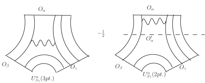
Figure 1: Graph of renormalization scheme independent structure constant.

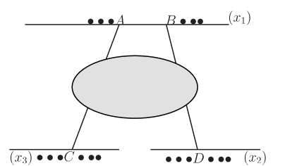
Figure 2: A schematic one loop diagram

3.1 One loop diagrams and the contributions

We will now explicitly evaluate the contribution of all possible diagrams at one loop that can contribute to the structure constants. As we have discussed earlier, the renormalization scheme independent contribution to the structure constants depend only on the combination given in (3). The gauge invariant single trace operators we consider consist of scalars built out of the 3 complex scalars of the beta deformed theory. Thus we can restrict our selves to examine diagrams of the type given in figure 2 with the letters $A,B,C,D$ belonging to any of the $3$ complex scalars and their conjugates. The shaded blob represents either the quartic interactions due to the scalar potential of (2) given in figures(4) and (5) or the gauge exchange given in figure(3(a)).

After the evaluation of the contribution of each of the diagrams to the structure constants we will compare the contribution of the same diagram to the coefficient of the anomalous dimension matrix in a two point function. By this comparison we demonstrate that the contribution to the structure constants by the same diagram is proportional to the anomalous dimension. This will establish that the contribution to the structure constants defined by (3.15) is essentially captured by the anomalous dimension Hamiltonian.

Note that by a simple large $N$ counting these diagrams are proportional to the factor $\frac{\lambda}{N}$ which we will suppress. Let us now examine the contribution of the diagrams to the structure constants one by one.

(i) $A=B=Z_{i}$ and $C=D=\bar{Z}_{i}$, $i=1,2,3$

We consider the set of diagrams with both the letters $A,B$ being $Z_{i}$ and the letters $C,D$ being $\bar{Z}_{i}$. $i$ can take any value $i=1,2,3$. The constant term from the quartic interaction for this diagram is obtained by extracting the finite term from

$$\tilde{Q}({\bf{i}};{\rm 3pt})=-\frac{2}{4}\left(\lim_{x_{2}\rightarrow x_{1}}\frac{\phi(r,s)}{x_{13}^{2}x_{24}^{2}}\right).$$ (3.17)

Here the $2/4$ arises from the normalization of the quartic potential in the scalar potential given in (2). The quartic contribution arises from the figures (4(c)) and (4(d)). $\phi(r,s)$ is given by the integral which appears in the quartic interaction

$$\int d^{4}u\frac{1}{(x_{1}-u)^{2}(x_{2}-u)^{2}(x_{3}-u)^{2}(x_{4}-u)^{2}}=\frac{\pi^{2}\phi(r,s)}{x_{13}^{2}x_{24}^{2}}$$ (3.18)

and $r,s$ are the conformal cross ratios defined by

$$r=\frac{x_{12}^{2}x_{34}^{2}}{x_{13}^{2}x_{24}^{2}},\qquad s=\frac{x_{14}^{2}x_{23}^{2}}{x_{13}^{2}x_{24}^{2}}.$$ (3.19)

The limit $x_{2}\rightarrow x_{1}$ is taken by setting $x_{2}-x_{1}=\epsilon\rightarrow 0$. Note that under this limit $r\rightarrow 0,s\rightarrow 1$. The expansion of the function $\phi(r,s)$ is known around this point . Substituting this expansion into (4(a)) we obtain

$$\tilde{Q}({\bf{i}};{\rm 3pt})=-\frac{2}{4}\frac{1}{x_{13}^{2}x_{14}^{2}}\left(\ln\left[\frac{x_{13}^{2}x_{14}^{2}}{x_{34}^{2}\epsilon^{2}}\right]+2\right).$$ (3.20)

The term proportional to the logarithm contributes to the logarithmic corrections in the 3 point functions arising from the anomalous dimension, while the constant term contributes to the structure constant. Thus the constant term from the 3 body interaction of the quartic potential is given by

$$Q({\bf{i}};{\rm 3pt})=-\frac{2}{4}\times 2.$$ (3.21)

Now we examine the same diagram but as a 2 body interaction. We thus have to evaluate

$$\hat{Q}({\bf{i}};{\rm 2pt})=-\frac{2}{4}\lim_{x_{1}\rightarrow x_{2},x_{3}\rightarrow x_{4}}\frac{\phi(r,s)}{x_{13}^{2}x_{24}^{2}},$$ (3.22)

where the limits are taken by setting $x_{1}\rightarrow x_{2}=\epsilon$, $x_{4}-x_{3}=\epsilon$ and then finally taking $\epsilon\rightarrow 0$. We can then extract the constant term from this using the expansions of the function $\phi(r,s)$. Performing this we obtain

$$Q({\bf{i}};{\rm 2pt})=Q({\bf{i}};{\rm 3pt})=-1.$$ (3.23)

Let us now proceed to the gauge exchange contribution to the 3 body interaction. This is obtained by extracting the finite terms from

$$\hat{G}({\bf{i}};{\rm 3pt})=-\frac{1}{2}\lim_{x_{1}\rightarrow x_{2}}H(x_{1},x_{2},x_{3},x_{4}).$$ (3.24)

Here the $1/2$ arises from the $\frac{1}{\sqrt{2}}$ in coupling in the covariant derivatives. The negative sign arises because two powers of $i$ in this interaction and $H$ is given by

$$H=(\partial_{1}-\partial_{3})\cdot(\partial_{2}-\partial_{4})\int\frac{d^{4}ud^{4}v}{\pi^{2}(2\pi)^{2}}\frac{1}{(x_{1}-u)^{2}(x_{3}-u)^{2}}\frac{1}{(u-v)^{2}}\frac{1}{(x_{2}-v)^{2}(x_{4}-v)^{2}}.$$ (3.25)

Setting $x_{1}-x_{2}=\epsilon$ and taking $\epsilon\rightarrow 0$ and keeping track of only the finite terms we obtain Alday:2005nd

$$G({\bf{i}};{\rm 3pt})=-\frac{1}{2}\times 2.$$ (3.26)

Note that as discussed in Alday:2005nd there are terms in the limit (3.24) which apparently seems to violate conformal invariance. On summing all such terms from the contributions in the $3$ terms of (3) it can be shown that they vanish. Let us now evaluate the contribution of the gauge exchange diagram but now thought of as arising from a two point function. We have extract the finite terms from

$$\hat{G}({\bf{i}};{\rm 2pt})=-\frac{1}{2}\lim_{x_{1}\rightarrow x_{2},x_{3}\rightarrow x_{4}}H(x_{1},x_{2},x_{3},x_{4}).$$ (3.27)

Evaluating this limit and extracting the finite terms as done in Alday:2005nd we obtain

$$G({\bf{i}};{\rm 2pt})=-\frac{1}{2}\times 6.$$ (3.28)

Putting the contributions of the quartic interaction and the gauge exchange together and evaluating the renormalization scheme independent contribution to the structure constant we obtain

$$C({\bf{i}}) = Q({\bf{i}};{\rm 3pt})+H({\bf{i}};{\rm 3pt})-\frac{1}{2}(Q({\bf{i}};,{\rm 2pt})+H({\bf{i}};{\rm 2pt})),$$

$$= 0.$$

Note that the contribution from the diagrams with $A=B=\bar{Z}_{i}$ and $C=D=\bar{Z}_{i}$, that is with the $Z$’s interchanged with the corresponding $\bar{Z}$ remains identical to the case discussed.

(ii) $A=D=Z_{i}$ and $B=C=\bar{Z}_{i}$, $i=1,2,3$

Having explained in detail the contributions that make up diagram (i ), we now just outline the results for the remaining diagrams. The contribution of quartic interaction arises from figures (4(a)) and (4(b)) . This results in the following

$$Q({\bf{ii}};{\rm 3pt})-\frac{1}{2}Q({\bf{ii}};{\rm 2pt})=\frac{1}{2}.$$ (3.30)

The gauge exchange diagram gives

$$G({\bf{ii}};{\rm 3pt})-\frac{1}{2}G({\bf{ii}};{\rm 2pt})=\frac{1}{2}.$$ (3.31)

Thus the total contribution of this diagram to the structure constant is

$$C({\bf{ii}})=1.$$ (3.32)

As we have mentioned earlier, the same contribution arises from the complex conjugated diagram.

(iii) $A=Z_{i},B=Z_{j},C=\bar{Z}_{i},D=\bar{Z}_{j}$ and $i\neq j$, $i=1,2,3$

The contribution of the quartic interaction here arises from both the F-term and D-terms in the scalar potential. The D-term contribution arise from figures (4(c)) and (4(d)) and F contribution arise from (5(b))(shown for the case of $i=1,j=2$) and (5(a))( shown for the case of for $i=2,j=1$) This results in the following

$$Q({\bf{iii}};{\rm 3pt})-\frac{1}{2}Q({\bf{iii}};{\rm 2pt})=\frac{1}{2}.$$ (3.33)

The gauge exchange diagram results in

$$G({\bf{iii}};{\rm 3pt})-\frac{1}{2}G({\bf{iii}};{\rm 2pt})=\frac{1}{2}.$$ (3.34)

Thus the total contribution to the structure constant is

$$C({\bf{iii}})=1.$$ (3.35)

Again here the complex conjugate of this diagram gives the same contribution to the structure constant.

(iv) $A=Z_{i},B=\bar{Z}_{j},C=\bar{Z}_{i},D=Z_{j}$ and $i\neq j$, $i=1,2,3$

The contribution of the quartic interaction arises from diagram in figure(4(b)). In fact this figure gives a factor of 2 due to the two possible ways of Wick contraction in the D-terms. There is no contribution from the F-term. This results in the following contribution to the structure constant

$$Q({\bf{iv}};{\rm 3pt})-\frac{1}{2}Q({\bf{iv}};{\rm 2pt})=\frac{1}{2}.$$ (3.36)

The gauge exchange contribution results in

$$G({\bf{ii}},{\rm 3pt})-\frac{1}{2}G({\bf{ii}},{\rm 2pt})=\frac{1}{2}.$$ (3.37)

Thus the total contribution to the structure constant is

$$C({\bf{iv}})=1.$$ (3.38)

Again here the complex conjugate of this diagram results in same contribution to the structure constant.

(v) $A=Z_{i},B=\bar{Z}_{i},C=\bar{Z}_{j},D=Z_{j}$ and $i\neq j$, $i=1,2,3$

For this case the D-type terms of figures (4(a))(with an extra factor of 2 for two ways of Wick contraction) contribute to the quartic interaction. This results in

$$Q({\bf{v}};{\rm 3pt})-\frac{1}{2}Q({\bf{v}};{\rm 2pt})=\frac{1}{2}.$$ (3.39)

There is no contribution from the gauge exchange interaction in this diagram. This is because one does not allow self contractions between the letters belonging to the same operator. Therefore the total contribution is given by

$$C({\bf{v}})=\frac{1}{2}.$$ (3.40)

The complex conjugate of this diagram also yields the same result.

(vi) $A=Z_{i},B=\bar{Z}_{i},C=Z_{j},D=\bar{Z}_{j}$ and $i\neq j$, $i=1,2,3$

D-type figures (4(c)) and (4(d)) contributes to the quartic interaction. F contribution arise from figure (5(a))(for $i=1,j=2$) and (5(b))(for $i=2,j=1$) This results in

$$Q({\bf{vi}};{\rm 3pt})-\frac{1}{2}Q({\bf{vi}};{\rm 3pt})=\frac{1}{2}.$$ (3.41)

Again for this diagram there is no contribution from the gauge exchange. Thus the structure constant contribution is

$$C({\bf{vi}})=\frac{1}{2}.$$ (3.42)

Here also the complex conjugate of this diagram yields the same result.

(vii) $A=Z_{1},B=Z_{2},C=\bar{Z}_{2},D=\bar{Z}_{1}$ and cyclic

Here only the F-type term contributes to the quartic interaction and there is no gauge exchange contribution. The diagram which contributes is (5(c)). This results in the following

$$C({\bf{vii}})=Q({\bf{vii}};{\rm 3pt})-\frac{1}{2}Q({\bf{vii}};{\rm 2pt})=-e^{i\beta}.$$ (3.43)

All diagrams related to this by the cyclic replacement of $Z_{1}\rightarrow Z_{2}\rightarrow Z_{3}\rightarrow Z_{1}$ yields the same result. Further the complex conjugate of this diagram also yields the same result.

(viii) $A=Z_{2},B=Z_{1},C=\bar{Z}_{1}D=\bar{Z}_{2}$ and cyclic

Only the F-type term given in figure (5(d)) contributes, there is no contribution from the gauge exchange. This results in

$$C({\bf{vii}})=Q({\bf{viii}};{\rm 3pt})-\frac{1}{2}Q({\bf{viii}};{\rm 2pt})=-e^{-i\beta}.$$ (3.44)

Again all diagram related to this one by cyclic replacements and well as the conjugate diagram yields the same result for the structure constant.

(ix) $A=Z_{1},B=\bar{Z}_{2},C=Z_{2},D=\bar{Z}_{1}$ and cyclic

The F-type term given in figure(5(d)) contributes and there is no contribution from the gauge exchange term. Thus the structure constant contribution from this class of diagrams is given by

$$C({\bf{ix}})=Q({\bf{ix}};{\rm 3pt})-\frac{1}{2}Q({\bf{ix}};{\rm 2pt})=-e^{-i\beta}.$$ (3.45)

All diagrams which are obtained by cyclic replacements as well as the conjugate diagrams result in the same structure constant.

(x) $A=Z_{2},B=\bar{Z}_{1},C=Z_{1},D=\bar{Z}_{2}$ and cyclic

For these class of diagrams only the F-type term given in figure(5(c)) contributes and there is no contribution from the gauge exchange term. The contribution to the structure constant is given by

$$C({\bf{x}})=Q({\bf{x}};{\rm 3pt})-\frac{1}{2}Q({\bf{x}};{\rm 2pt})=-e^{i\beta}.$$ (3.46)

Again all diagrams obtained by cyclic replacements as well as the conjugate diagrams result in the same structure constant.

Now we can compare the evaluation of the contributions to the renormalization scheme independent structure constant to that of the anomalous dimension Hamiltonian given in the appendix A diagram by diagram . We see that the contribution to the structure constant for each diagram is $-1/2$ that of the anomalous dimension Hamiltonian. This shows that the one loop corrections to structure constants are indeed controlled by the anomalous dimension Hamiltonian. When all the contributions to the structure constant in given three point functions are put together these will organize into combinations of the anomalous dimensions of the respective operators involved in the three point function. This is identical to how the coefficients of the logarithms in the three point function organize into combinations of the anomalous dimensions of the respective operators.

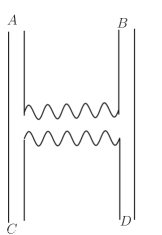
(a) Gauge interaction

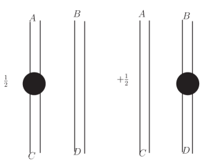
(b) Self energy: fermions and bosons in loops

Figure 3: Gauge exchanges and self energies

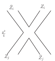
(a)

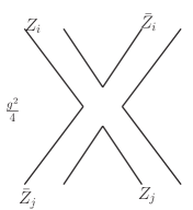
(b)

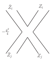
(c)

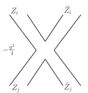
(d)

Figure 4: Possible D-type Quartic Interactions. Rotations of the diagrams in the plane are allowed in Wick contractions

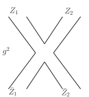
(a)

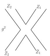
(b)

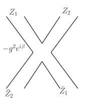
(c)

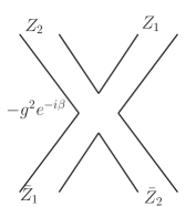
(d)

Figure 5: Possible F-type Quartic Interactions. Rotations of the diagrams in the plane are allowed in Wick contractions. Cyclic replacements of $Z_{1},Z_{2}$ are other possible diagrams

3.2 Non-renormalization of structure constants of chiral primaries

It is known that the structure constants of $3$ chrial primaries in ${\cal N}=4$ Yang-Mills do not get renormalized at all orders in the coupling Lee:1998bxa . For a proof involving ${\cal N}=4$ harmonic superspace see Howe:1998zi . A similar question for the case of the $\beta$ deformed ${\cal N}=1$ Yang-Mills is yet to be investigated. For arbitrary values of the deformation parameter $\beta$, the chiral primaries have the following $U(1)$ charges

$$(k,0,0),\qquad(0,k,0),\qquad(0,0,k),\qquad(k,k,k)$$ (3.47)

An argument to indicate that the three point function involving chiral primaries only of the first three type are not renormalized at one loop was given in Freedman:2005cg .

Let us now use the result of the previous section to show how three point function involving any chiral primaries in (3.47) including that with $U(1)$ charge $(k,k,k)$ are not renormalized at one loop in the t’Hooft limit. We have shown that the finite corrections to structure constants at one loop organized themselves to the anomalous dimensions of the operators involved in the three point function. If the three operators involved are chiral primaries then this correction vanishes. As mentioned in the discussion below equation (3.15), there is an additional contribution to the structure constant at one loop. This arises if the operators involved mix at one loop which can be found by examining the two loop anomalous dimension Hamiltonian. If the operators are all chiral primary, there is no mixing and hence this contribution also vanishes. Thus there are are no corrections at one loop to the structure constants involving only chiral primaries.

Let us examine the chiral primary with charge $(k,k,k)$ in more detail. The explicit construction of this operator in the planar limit is by Freedman:2005cg

$${O}_{(k,k,k)}=\sum_{\pi}c_{\pi}{\rm Tr}\left(\pi Z_{1}^{k}Z_{2}^{k}Z_{3}^{k}\right),$$ (3.48)

where

$$c_{\pi}=\frac{\bar{q}^{k_{\pi}}}{s_{\pi}},\qquad\bar{q}=e^{-i\beta}.$$ (3.49)

$k_{\pi}$ is the number of permutations required to obtain that term from the configuration of

$${\rm Tr}(Z_{1}^{k}Z_{2}^{k}Z_{3}^{k}).$$ (3.50)

$s_{\pi}$ is the symmetry factor which counts the number of repeated arrays, see Freedman:2005cg for a detailed discussion of how this symmetry factor is evaluated. The sum in (3.48) runs over all the permutations. Note that when $\beta=0$, it reduces to the chiral primary of ${\cal N}=4$. Let us explicitly write down the operators at the first two levels .

$${O}_{(1,1,1)} = {\rm Tr}(Z_{1}Z_{2}Z_{3})+\bar{q}^{2}{\rm Tr}(Z_{1}Z_{2}Z_{3}),$$ (3.51)

$${O}_{(2,2,2)} = {\rm Tr}\left(Z_{1}^{2}Z_{2}^{2}Z_{3}^{2}+\bar{q}^{2}Z_{1}^{2}Z_{2}Z_{3}Z_{2}Z_{3}+\bar{q}^{4}Z_{1}^{2}Z_{2}Z_{3}^{2}Z_{2}+Z_{1}^{2}Z_{3}Z_{2}^{2}Z_{3}\right.$$

$$\bar{q}^{6}Z_{1}^{2}Z_{3}Z_{2}Z_{3}Z_{2}+\bar{q}^{8}Z_{1}^{2}Z_{3}^{2}Z_{2}^{2}+\bar{q}^{2}Z_{3}^{2}Z_{1}Z_{2}Z_{1}Z_{2}+\bar{q}^{4}Z_{1}Z_{2}Z_{1}Z_{3}Z_{2}Z_{3}$$

$$\bar{q}^{6}Z_{3}^{2}Z_{2}Z_{1}Z_{2}Z_{1}+\bar{q}^{4}Z_{1}Z_{2}^{2}Z_{1}Z_{3}^{2}+\bar{q}^{6}Z_{2}^{2}Z_{1}Z_{3}Z_{1}Z_{3}+\frac{1}{2}\bar{q}^{2}Z_{1}Z_{2}Z_{3}Z_{1}Z_{2}Z_{3}$$

$$\left.\bar{q}^{4}Z_{2}Z_{1}Z_{2}Z_{3}Z_{1}Z_{3}+\bar{q}^{4}Z_{1}Z_{3}Z_{1}Z_{2}Z_{3}+\bar{q}^{2}Z_{2}^{2}Z_{3}Z_{1}Z_{3}Z_{1}+\frac{1}{2}\bar{q}^{6}Z_{1}Z_{3}Z_{2}Z_{1}Z_{3}Z_{2}\right).$$

Consider the three point function

$$\langle{O}_{(k,k,k)}\bar{O}_{(k_{1},k_{1},k_{1})}\bar{O}_{(k_{2},k_{2},k_{2})}\rangle$$ (3.52)

where $k=k_{1}+k_{2}$. We have shown that this three point function does not get renormalized at one loop. There is another important property of this three point function. The tree level 3 point function is independent of $\beta$ in the planar limit. This can seen by the fact that in the planar limit there is a non-zero contribution from the Wick contraction only if the letters in ${O}_{(k,k,k)}$ are aligned with the other two. Let us focus on one particular term $T_{k}$ in operator ${O}_{(k,k,k)}$ when the Wick contraction is non-zero with the first terms ${\rm Tr}(\bar{Z}_{1}^{k_{1}}\bar{Z}_{2}^{k_{1}}\bar{Z}_{3}^{k_{1}}),{\rm Tr}(\bar{Z}_{1}^{k_{2}}\bar{Z}_{2}^{k_{2}}\bar{Z}_{3}^{k_{2}})$ of operators $\bar{O}_{(k_{1},k_{1},k_{1})},\bar{O}_{(k_{2},k_{2},k_{2})}$ respectively. We call these terms $T_{k_{1}}$ and $T_{k_{2}}$ . Now let $S_{k}$, $S_{k_{1}}$, $S_{k_{2}}$ be another set of terms in each of the operators which have non-zero overlap. The number of permutations to obtain $S_{k}$ from $T_{k}$ must be equal to the total number of permutations to obtain $S_{k_{1}}$ and $S_{k_{2}}$ from $T_{k_{1}}$ and $T_{k_{2}}$ respectively. From the construction of operators given in (3.48), this implies that the relative phase between the contribution of the $T$’s to the three point function and the contribution of the $S$’s to the three point function vanishes. Note that the phases in $\bar{O}_{(k_{1},k_{1},k_{1})},\bar{O}_{(k_{2},k_{2},k_{2})}$ involve $q$ while the phases in ${O}_{(k,k,k)}$ involve $\bar{q}$. Thus other than an over all phase there are no relative phases between any terms in the contractions which give rise to the tree level three point function given in (3.52). This over all phase can be removed by an appropriate redefinition of say the first operator. One can explicitly check this for the the case of $k=2,k_{1}=k_{2}=1$ with the operators given in (3.51). Therefore we conclude that the tree level structure constant in the planar limit is independent of the deformation $\beta$.

We summarize the properties of the three point function given in (3.52).

1. The structure constant does not receive corrections at one loop in the t’ Hooft limit.

2. The tree level planar structure constant is independent of the deformation $\beta$.

3. Properties (1) and (2) imply that the structure constant (3.52) is equal to that in ${\cal N}=4$ Yang-Mills to one loop in t ’Hooft coupling.

If these properties were to hold to all orders in t’Hooft coupling we should expect to see these properties in the Lunin-Maldacena geometry which is the strong coupling dual of the beta deformed theory.

4 Structure constants from the Lunin-Maldacena background

Motivated by the arguments in the previous section we turn towards evaluating structure constants in the Lunin-Maldacena background which is the strong coupling dual. We will use the method developed by Zarembo:2010rr for evaluating the three point function. There has been holographic computations of three point functions of a chiral primary with operators dual to large semi-classical strings in the Lunin-Maldacena background by Ahn:2011dq ; Alizadeh:2011yt . The chiral primary involved was restricted to to be dual to the dilaton in these works . Our primary focus is on evaluating the structure constants of the three chiral primary given in (3.52) and showing that the result is independent of the deformation and it reduces to the same evaluated for the holographic dual of ${\cal N}=4$ Yang-Mills. We then evaluate the structure constants of the R-current with semi-classical string states and verify a Ward-identity. We also evaluate the structure constants of the chiral primary with charge $(k,k,k)$ with other semi-classical string states.

The first step is to evaluate the supergravity mode dual to the chiral primary $O_{(k,k,k)}$. This is done in section 4.1. Then in section 4.2 we use this to evaluate the three point function given in (3.52) using the method of Zarembo:2010rr . We show that the answer is identical to that of the ${\cal N}=4$ result. This result together with the one loop results of the previous section suggests that the the three point function in (3.52) is protected by a non-renormalization theorem.

4.1 The $(k,k,k)$ chiral primary at strong coupling

In this section we will write down the gravity fluctuations which is dual to the chiral primary state ${O}_{(k,k,k)}$ in the Lunin-Maldacena background. Note that the Lunin-Maldacena background is obtained by performing a TsT transformation on the $AdS_{5}\times S^{5}$ geometry Lunin:2005jy ; Frolov:2005dj . The strategy we adopt is the following:

1. Identify the chiral primary fluctuations corresponding to the operator with $U(1)$ charge ${(k,k,k)}$ in the $AdS_{5}\times S^{5}$ background.

2. Show that the background together with the fluctuation preserves an $U(1)$ isometry so that the TsT transformation can be performed.

3. Perform the TsT transformation on the background with the fluctuations and obtain the Lunin-Maldacena background along with the fluctuations. This yields the super gravity mode dual to the operator ${O}_{(k,k,k)}$.

4. As a consistency check we verify that the equations of motion of the fluctuations in the Lunin-Maldacena background reduces to that of Klein-Gordan field with (mass)${}^{2}=k(k-4)$.

Before proceeding let us first review how the Lunin-Maldacena background is obtained by performing a TsT transformation on the $AdS_{5}\times S^{5}$ background. We follow Frolov:2005dj . The $AdS_{5}\times S^{5}$ background is given by

$$ds^{2}=\frac{1}{z^{2}}(dx^{2}+dz^{2})+d\Omega_{5}^{2},\\$$

where $d\Omega_{5}^{2}$ is the metric on the sphere. Let us parametrize the sphere as

$$d\Omega_{5}^{2}=\sum_{i}^{3}dr_{i}^{2}+\sum_{i}^{3}r_{i}^{2}d\tilde{\tilde{\phi}}_{i}^{2},$$ (4.53)

$$r_{1}^{2}+r_{2}^{2}+r_{3}^{2}=1,$$

$$r_{1}=\cos\alpha\equiv c_{\alpha},\qquad r_{2}=\sin\alpha\cos\theta\equiv s_{\alpha}c_{\theta},\qquad r_{3}=\sin\alpha\sin\theta\equiv s_{\alpha}s_{\theta}.$$

There is also the background $RR$ 4-from which is given by

$$C_{4}=4(w_{4}+w_{1}\wedge d\tilde{\tilde{\phi}}_{1}\wedge d\tilde{\tilde{\phi}}_{2}\wedge d\tilde{\tilde{\phi}}_{3}),$$ (4.54)

where

$$dw_{4}=\omega_{AdS_{5}},\qquad dw_{1}=\sqrt{g_{s^{5}}}d\alpha\wedge d\theta=c_{\alpha}s^{3}_{\alpha}s_{\theta}c_{\theta}d\alpha\wedge d\theta,$$ (4.55)

$$w_{1}=\frac{1}{4}s^{4}_{\alpha}s_{\theta}c_{\theta}d\theta.$$

The dilaton background is constant and we have set $e^{\Phi}=1$ and the radius of $AdS$ to be unity. We will re-introduce the constant mode of the dilaton and the radius of $AdS$ in the sigma model coupling as in Zarembo:2010rr .

The TsT dual is obtained as follows Frolov:2005dj :

1. First perform the following co-ordinate transformation

   $$\tilde{\tilde{\phi}}_{1}=\tilde{\tilde{\varphi}}_{3}-\tilde{\tilde{\varphi}}_{2},\qquad\tilde{\tilde{\phi}}_{2}=\tilde{\tilde{\varphi}}_{3}+\tilde{\tilde{\varphi}}_{2}+\tilde{\tilde{\varphi}}_{1},\qquad\tilde{\tilde{\phi}}_{2}=\tilde{\tilde{\varphi}}_{3}-\tilde{\tilde{\varphi}}_{1}.$$ (4.56)

   Substituting these transformations in the metric of the $S^{5}$ we see that the metric is no longer diagonal. The RR 4-form also is written in these co-ordinates.

2. We then perform T-duality along the $\tilde{\tilde{\varphi}}_{1}$ direction. This is done by applying the standard T-duality rules given in Meessen:1998qm . We are now in the type IIA theory. Let us now label the $3$ circles as $\tilde{\varphi}_{1},\tilde{\varphi}_{2}$ and $\tilde{\varphi}_{3}$.

3. Then the following shift is done by replacing

   $$\tilde{\varphi}_{2}\rightarrow\tilde{\varphi}_{2}+\gamma\tilde{\varphi}_{1}.$$ (4.57)

4. The next step is to again perform a T-duality along the $\tilde{\varphi}_{1}$ direction. Now we are back in type IIB theory, we label the circles now as $\varphi_{1},\varphi_{2},\varphi_{3}$.

5. Finally we undo the co-ordinate transformation in (4.56) by performing the inverse transformation given by

   $$\varphi_{1}=\frac{\phi_{2}+\phi_{1}-2\phi_{3}}{3},\qquad\varphi_{2}=\frac{\phi_{2}+\phi_{3}-2\phi_{1}}{3},\qquad\varphi_{3}=\frac{\phi_{1}+\phi_{2}+\phi_{3}}{3}.$$ (4.58)

The result of this TsT transformation is the following solution of type IIB gravity in the string frame

$$ds^{2} = \frac{1}{z^{2}}\left(dx^{2}+dz^{2}\right)+\sum_{i=1}^{3}(dr_{i}^{2}+Gr_{i}^{2}d\phi_{i}^{2})+\gamma^{2}Gr_{1}^{2}r_{2}^{2}r_{3}^{2}\sum_{i}d\phi_{i}\sum_{j}d\phi_{j},$$ (4.59)

$$G = \frac{1}{1+\gamma^{2}(r_{1}^{2}r_{2}^{2}+r_{2}^{2}r_{3}^{2}+r_{3}^{2}r_{1}^{2})}.$$

The background also contains the dilaton which is given by

$$\Phi=\frac{1}{2}\log G.$$ (4.60)

The anti-symmetric NS-NS 2-form fields which are turned on are given by

$$b_{\phi_{1}\phi_{2}}=G\gamma r_{1}^{2}r_{2}^{2},\quad b_{\phi_{2}\phi_{3}}=G\gamma r_{2}^{2}r_{3}^{2},\quad b_{\phi_{3}\phi_{1}}=G\gamma r_{3}^{2}r_{1}^{2}.$$ (4.61)

The component of the RR 2-form fields which are turned on are given by following transformation rules

$$C^{2\gamma}_{\alpha\theta} = \gamma\left(-C^{4}_{\alpha\theta{\tilde{\tilde{\phi}}_{2}}{\tilde{\tilde{\phi}}_{3}}}+C^{4}_{\alpha\theta{\tilde{\tilde{\phi}}_{1}}{\tilde{\tilde{\phi}}_{3}}}-C^{4}_{\alpha\theta{\tilde{\tilde{\phi}}_{1}}{\tilde{\tilde{\phi}}_{2}}}\right),$$ (4.62)

$$C^{2\gamma}_{\theta\phi_{i}} = -\gamma C^{4}_{\theta{\tilde{\tilde{\phi}}_{1}}{\tilde{\tilde{\phi}}_{2}}{\tilde{\tilde{\phi}}_{3}}},$$ (4.63)

$$C^{2\gamma}_{\alpha\phi_{i}} = -\gamma C^{4}_{\alpha{\tilde{\tilde{\phi}}_{1}}{\tilde{\tilde{\phi}}_{2}}{\tilde{\tilde{\phi}}_{3}}}.$$ (4.64)

These transformation rules can be obtained by a straight forward application of T-duality rules given in Meessen:1998qm . Here the values for the components on the right hand of the above equations can be read out from the expression for the 4-form given in (4.54). Implementing the RR transformation rules we find the following RR 2-form components turned on

$$C^{2\gamma}_{\theta\phi_{i}}=-\gamma\sin^{4}\alpha\sin\theta\cos\theta.$$ (4.65)

Finally applying the TsT rules we find that the anti-symmetric 4-form RR field is given by

$$C=4(\omega_{4}+Gw_{1}d\phi_{1}\wedge d\phi_{2}\wedge d\phi_{3}),$$ (4.66)

where

$$d\omega_{4}=\omega_{AdS_{5}},\qquad\omega_{1}=\frac{1}{4}\sin^{4}\alpha\sin\theta\cos\theta d\theta$$ (4.67)

$$d\omega_{1}=\cos\alpha\sin^{3}\alpha\sin\theta\cos\theta=\sqrt{g_{S}^{5}}d\alpha\wedge d\theta.$$

Note that the fields of background after the TsT transformation are all parametrized by the deformation parameter $\gamma$. This background satisfies the type IIB equations of motion which can be obtained from the action

$$S = \frac{1}{2\kappa_{10}^{2}}\int d^{10}x\sqrt{-g_{E}}\left(R-\frac{1}{2}\partial_{M}\Phi\partial^{M}\Phi-\frac{e^{-\Phi}H_{3}^{2}}{2.3!}-\frac{1}{2}e^{2\Phi}F_{1}^{2}-\frac{e^{\Phi}F_{3}^{2}}{2.3!}-\frac{1}{4.5!}F_{5}^{2}\right)$$ (4.68)

$$-\frac{1}{2\kappa_{10}^{2}}\int C_{4}\wedge H_{3}\wedge F_{3}.$$

Note that this action is written in Einstein frame and $2\kappa_{10}^{2}=(2\pi)^{7}\alpha^{\prime 4}$. The relation between the string frame and the Einstein frame is given by

$$g_{MN}^{E}=e^{-\Phi/2}g_{MN}^{S}.$$ (4.69)

The equations of motion is further supplemented by the self duality constraint on the $5$-form field strength. When $\gamma=0$, the solution given in (4.59), (4.60), (4.61), (4.65) and (4.66) reduces to the usual $AdS_{5}\times S^{5}$. The deformation $\gamma$ is identified with $\beta/2\pi$ of the beta deformed theory Lunin:2005jy .

Let us now examine the fluctuations which correspond to the chiral primaries in the $AdS_{5}\times S^{5}$ background Kim:1985ez ; Lee:1998bxa . We perturb the metric and the RR 4-form by

$$g_{MN}=g_{MN}^{(0)}+\varepsilon h_{MN},\qquad\tilde{C}_{4}=C_{4}^{(0)}+\varepsilon a_{4},$$ (4.70)

where the non-zero components of the perturbations $h_{MN}$ and $a_{4}$ are defined by Lee:1998bxa

$$h_{mn} = \frac{2}{{\cal N}_{k}(k+1)}Y_{I}[2\nabla_{m}\nabla_{n}-k(k-1)g_{mn}]s_{I}(x,z),$$ (4.71)

$$h_{\alpha\beta} = \frac{2kg_{\alpha\beta}Y_{I}s_{I}(x,z)}{{\cal N}_{k}},$$ (4.72)

$$a_{\alpha\beta\gamma\delta} = -4\sqrt{g_{s^{5}}}\frac{\epsilon_{\alpha\beta\gamma\delta\epsilon}\nabla^{\epsilon}Y_{I}s_{I}(x,z)}{{\cal N}_{k}},$$ (4.73)

$$a_{mnpr} = 4\sqrt{g_{AdS_{5}}}\frac{\epsilon_{mnprs}Y_{I}\nabla^{s}s_{I}(x,z)}{{\cal N}_{k}}.$$ (4.74)

The labels $m,n,\cdots$ take values from $0,1,\cdots 4$ which label the $AdS_{5}$ directions. The labels $\alpha,\beta,\cdots$ take values from $5,6,\cdots 9$ which label the $S^{5}$ directions. $Y_{I}$ are spherical harmonics on the $S^{5}$, I labels the various spherical harmonics. The spherical harmonics satisfy the equation

$$\nabla_{\alpha}\nabla^{\alpha}Y_{I}+k(k+4)Y_{I}=0$$ (4.76)

Thus $k$ refers to the rank of the spherical harmonic. For future reference we write down the non-zero components of the RR 4-form on $S^{5}$ along with the fluctuations explicitly:

$$C^{4}_{\theta{\tilde{\tilde{\phi}}_{1}}{\tilde{\tilde{\phi}}_{2}}{\tilde{\tilde{\phi}}_{3}}} = s^{4}_{\alpha}s_{\theta}c_{\theta}-4\varepsilon\frac{\sqrt{g_{S^{5}}}}{{\cal N}_{k}}s_{I}\partial_{\alpha}Y_{I},$$ (4.77)

$$C^{4}_{\alpha\tilde{\tilde{\phi}}_{1}\tilde{\tilde{\phi}}_{2}\tilde{\tilde{\phi}}_{3}} = 4\varepsilon\frac{\sqrt{g_{S^{5}}}}{{\cal N}_{k}}s_{I}\partial_{\theta}Y_{I}g^{\theta\theta},$$

$$C^{4}_{\alpha\theta{\tilde{\tilde{\phi}}_{2}}{\tilde{\tilde{\phi}}_{3}}} = -4\varepsilon\frac{\sqrt{g_{S^{5}}}}{{\cal N}_{k}}s_{I}\partial_{\tilde{\tilde{\phi}}_{1}}Y_{I}g^{\tilde{\tilde{\phi}}_{1}\tilde{\tilde{\phi}}_{1}},$$

$$C^{4}_{\alpha\theta\tilde{\tilde{\phi}}_{1}\tilde{\tilde{\phi}}_{3}} = 4\varepsilon\frac{\sqrt{g_{S^{5}}}}{{\cal N}_{k}}s_{I}\partial_{\tilde{\tilde{\phi}}_{2}}Y_{I}g^{\tilde{\tilde{\phi}}_{2}\tilde{\tilde{\phi}}_{2}},$$

$$C^{4}_{\alpha\theta\tilde{\tilde{\phi}}_{1}\tilde{\tilde{\phi}}_{2}} = -4\varepsilon\frac{\sqrt{g_{S^{5}}}}{{\cal N}_{k}}s_{I}\partial_{\tilde{\tilde{\phi}}_{3}}Y_{I}g^{\tilde{\tilde{\phi}}_{3}\tilde{\tilde{\phi}}_{3}},$$

with $g^{\alpha\alpha}=1,g^{\theta\theta}=\operatorname{cosec}^{2}{\alpha},g^{\tilde{\tilde{\phi}}_{i}\tilde{\tilde{\phi}}_{i}}=r_{i}^{-2}$ $(i=1,2,3)$. A simple example of a spherical harmonic on $S^{5}$ is given by

$$Y_{1}=\left(\frac{r_{1}}{\sqrt{2}}\right)^{k}\exp(ik\tilde{\tilde{\phi}}_{1}).$$ (4.78)

This spherical harmonic carries a charge $k$ along the direction $\tilde{\tilde{\phi}}_{1}$. Our conventions for the $\epsilon$ tensor are $\epsilon_{01234}=\epsilon_{56789}=1$. Now expanding the type IIB equations of motion to the linear order in fluctuation about the $AdS_{5}\times S^{5}$ background it can be seen that the amplitude of the fluctuations $s_{I}$ satisfy the minimally coupled massive scalar field in $AdS_{5}$ which is given by

$$\nabla_{m}\nabla^{m}s_{I}-k(k-4)s_{I}=0.$$ (4.79)

The normalization ${\cal N}_{k}$ is determined by holographically evaluating the two point function of the dual operator to this fluctuation and demanding it to be unity. For the spherical harmonic given in (4.78) this results in the following Zarembo:2010rr .

$$({\cal N}_{k}^{(1)})^{2}=\frac{N^{2}k(k-1)}{2^{k-3}\pi^{2}(k+1)^{2}}.$$ (4.80)

The superscript here refers to the fact that the normalization corresponds to the harmonic in (4.78). Note that the fluctuations satisfy the minimally coupled scalar equation in (4.79) with (mass)${}^{2}=k(k-4)$ .The $U(1)$ charge carried by the spherical harmonic in (4.78) is given in $(k,0,0)$. These two facts allow us to conclude that this supergravity mode is dual to the chiral primary ${\rm Tr}(Z_{1}^{k})$.

We now examine a chiral primary fluctuation in the $AdS_{5}\times S^{5}$ background which preserves the $U(1)$ isometry along $\tilde{\varphi}_{1}$ on which the $T$ duality is done. Note that the spherical harmonic given in (4.78) does not preserve the $U(1)$ isometry. The reason is that after the shift $\tilde{\varphi}_{2}\rightarrow+\gamma\tilde{\varphi}_{1}$, the fluctuation depends on the direction $\tilde{\varphi}_{1}$ and thus breaks the $U(1)$ isometry. The following spherical harmonic of rank $k$ preserves the $U(1)$ isometry.

$$Y_{2}=\frac{1}{2^{\frac{k}{2}}}(r_{1}r_{2}r_{3})^{\frac{k}{3}}\exp\left(\frac{ik}{3}(\tilde{\tilde{\phi}}_{1}+\tilde{\tilde{\phi}}_{2}+\tilde{\tilde{\phi}}_{3})\right).$$ (4.81)

Here $k$ is a multiple of $3$ so that the the function is periodic in the angles. Using the co-ordinate transformation in (4.56) we see that this harmonic just depends on the angle $\tilde{\varphi}_{3}$. Thus it preserves the $U(1)$ isometry along which the TsT transformation is done. From the $U(1)$ quantum numbers of this harmonic we see that it is dual to the operator ${O}_{\frac{k}{3}\frac{k}{3}\frac{k}{3}}$. Before proceeding we will determine normalization constant ${\cal N}_{k}^{(2)}$ corresponding to the harmonic in (4.81). The normalization is determined by requiring that the holographic two point function be normalized to unity. From the analysis of Lee:1998bxa we see that the normalization satisfies the following property

$$({\cal N}_{k}^{(I)})^{2}=f(k)z_{I}(k),$$ (4.82)

where $f(k)$ is quantity independent of the choice of spherical harmonics. But $z_{I}(k)$ is given by Lee:1998bxa

$$\int Y_{I_{1}}Y_{I_{2}}=z(k)\delta^{I_{1}I_{2}}.$$ (4.83)

For the spherical harmonic given in (4.78) it can be seen that

$$z_{1}(k)=\frac{2^{-k}8\pi^{3}}{4(2+k)(k+1)}.$$ (4.84)

For the second choice of spherical harmonic given in (4.81) we obtain

$$z_{2}(k)=\frac{8\pi^{3}2^{-k/2}(\Gamma(1+k/3))^{3}}{4\Gamma(k+3)}.$$ (4.85)

Then from (4.82) one can write

$$({\cal N}_{k}^{(2)})^{2} = ({\cal N}_{k}^{(1)})^{2}\frac{z_{2}(k)}{z_{1}(k)}=({\cal N}_{k}^{(1)})^{2}\frac{(\Gamma(1+k/3))^{3}}{\Gamma(k+1)}.$$ (4.86)

We now consider the $AdS_{5}\times S^{5}$ background along with the fluctuations given in (4.71) with the harmonic (4.81). Since the full background preserves the $U(1)$ isometry we can perform the TsT transformation. The TsT transformation maps solutions of equations of motion to solutions. Thus the fluctuations obtained after the TsT transformation will satisfy the linearized equations of motion about the Lunin-Maldacena background if (4.79) is true. We now write down the fluctuations about the Lunin-Maldacena background obtained by performing the TsT transformation of the chiral primary corresponding to the harmonic in (4.81). The background metric and the fluctuations are given by

$$G_{mn} = g_{mn}+\epsilon\frac{2}{{\cal N}_{k}(k+1)}Y_{2}[2\nabla_{m}\nabla_{n}-k(k-1)g_{mn}]s_{2},$$ (4.87)

$$G_{\alpha\alpha} = 1+\varepsilon\frac{2kY_{2}s_{2}}{{\cal N}_{k}}$$

$$G_{\theta\theta} = \sin^{2}\alpha\left(1+\varepsilon\frac{2kY_{2}s_{2}}{{\cal N}_{k}}\right),$$

$$G_{\phi_{1}\phi_{1}} = G(r_{1}^{2}+\gamma^{2}r_{1}^{2}r_{2}^{2}r_{3}^{2})$$

$$+\varepsilon\frac{2kY_{2}s_{2}}{{\cal N}_{k}}\left(\gamma^{4}(r_{1}^{4}r_{2}^{4}r_{3}^{2}+r_{1}^{4}r_{2}^{2}r_{3}^{4}+r_{1}^{2}r_{2}^{4}r_{3}^{4})+\gamma^{2}(2r_{1}^{2}r_{2}^{2}r_{3}^{2}-r_{1}^{4}r_{2}^{2}-r_{1}^{4}r_{3}^{2})+r_{1}^{2}\right)G^{2},$$

$$G_{\phi_{2}\phi_{2}} = G(r_{2}^{2}+\gamma^{2}r_{1}^{2}r_{2}^{2}r_{3}^{2}),$$

$$+\varepsilon\frac{2kY_{2}s_{2}}{{\cal N}_{k}}\left(\gamma^{4}(r_{1}^{4}r_{2}^{4}r_{3}^{2}+r_{1}^{4}r_{2}^{2}r_{3}^{4}+r_{1}^{2}r_{2}^{4}r_{3}^{4})+\gamma^{2}(2r_{1}^{2}r_{2}^{2}r_{3}^{2}-r_{2}^{4}r_{1}^{2}-r_{2}^{4}r_{3}^{2})+r_{2}^{2}\right)G^{2},$$

$$G_{\phi_{3}\phi_{3}} = G(r_{3}^{2}+\gamma^{2}r_{1}^{2}r_{2}^{2}r_{3}^{2}),$$

$$+\varepsilon\frac{2kY_{2}s_{2}}{{\cal N}_{k}}\left(\gamma^{4}(r_{1}^{4}r_{2}^{4}r_{3}^{2}+r_{1}^{4}r_{2}^{2}r_{3}^{4}+r_{1}^{2}r_{2}^{4}r_{3}^{4})+\gamma^{2}(2r_{1}^{2}r_{2}^{2}r_{3}^{2}-r_{3}^{4}r_{1}^{2}-r_{3}^{4}r_{2}^{2})+r_{3}^{2}\right)G^{2},$$

$$G_{\phi_{1}\phi_{2}} = G\gamma^{2}r_{1}^{2}r_{2}^{2}r_{3}^{2},$$

$$+\varepsilon\frac{2kY_{2}s_{2}}{{\cal N}_{k}}\left(\gamma^{4}(r_{1}^{4}r_{2}^{4}r_{3}^{2}+r_{1}^{4}r_{2}^{2}r_{3}^{4}+r_{1}^{2}r_{2}^{4}r_{3}^{4})+3\gamma^{2}r_{1}^{2}r_{2}^{2}r_{3}^{2}\right)G^{2},$$

$$G_{\phi_{2}\phi_{3}} = G_{\phi_{1}\phi_{3}}=G_{\phi_{1}\phi_{2}}.$$

In the above equations and the rest of the paper it is understood that the normalization ${\cal N}_{k}$ refers to ${\cal N}_{k}^{(2)}$ which is given in (4.86). The background NS B-field along with the fluctuations are given by

$$B_{\phi_{1}\phi_{2}} = G\gamma r_{1}^{2}r_{2}^{2}+2\varepsilon\frac{2kY_{2}s_{2}}{{\cal N}_{k}}G^{2}\gamma r_{1}^{2}r_{2}^{2},$$ (4.88)

$$B_{\phi_{2}\phi_{3}} = G\gamma r_{2}^{2}r_{3}^{2}+2\varepsilon\frac{2kY_{2}s_{2}}{{\cal N}_{k}}G^{2}\gamma r_{2}^{2}r_{3}^{2},$$

$$B_{\phi_{3}\phi_{1}} = G\gamma r_{3}^{2}r_{1}^{2}+2\varepsilon\frac{2kY_{2}s_{2}}{{\cal N}_{k}}G^{2}\gamma r_{3}^{2}r_{1}^{2}.$$

The background dilaton with the fluctuation is given by

$$\Phi=\frac{{\rm Log}G}{2}+\varepsilon\frac{2kY_{2}s_{2}}{{\cal N}_{k}}(G-1).$$ (4.90)

The RR 2-form components with the fluctuations are given by the relations given in (4.62) on the RR 4-components before the TsT transformation given in (4.77). One can also obtain the RR 4-form along with the fluctuation after the TsT transformation. However as will be seen in the next section our analysis requires only the NS fields and their fluctuations.

As a simple check of the fact that we have got the right set of fluctuations note that for $\gamma=0$, the background as well as the fluctuations reduces to the situation in $AdS_{5}\times S^{5}$. As a further non-trivial consistency check we verify that the amplitude of the fluctuation $s_{2}$ satisfies the minimally coupled scalar equation in $AdS_{5}$ with (mass)${}^{2}=k(k-4)$. To do this we first examine the dilaton equation of type IIB. In the Einstein frame this is given by

$$\frac{1}{\sqrt{-g_{E}}}\partial_{M}(g^{MN}_{E}\sqrt{-g_{E}}\partial_{N}\Phi)=e^{2\Phi}F_{1}^{2}+\frac{1}{2.3!}(e^{\Phi}F_{3}^{2}-e^{-\Phi}H_{3}^{2}).$$ (4.91)

We then convert our background and the fluctuations given in (4.87), (4.88), 4.90 to the Einstein frame using (4.69). This is substituted in the equation of motion for the dilaton (4.91). We then expand the LHS of the equation to the linear order in $\varepsilon$. After a tedious manipulation using Mathematica it can indeed be shown that if the amplitude $s_{2}$ satisfies (4.79) then the type IIB dilaton equation is satisfied to the linear order in the fluctuations.

4.2 3-pt functions of chiral primaries at strong coupling

Having constructed the super-gravity mode dual to the chiral primary operator ${\cal O}_{kkk}$ we are in a position to evaluate the structure constants of three chiral primaries defined in (3.52). For this purpose we will use the method developed by Zarembo:2010rr which evaluates the structure constant of a super-gravity mode with two semi-classical strings states in terms of a world-sheet amplitude. Let the metric and the NS-B field fluctuations of the super-gravity mode in the string frame be given by $h_{MN}^{I}$ and $b_{MN}^{I}$, where $I$ labels the mode. Then the structure constant is extracted from the amplitude Zarembo:2010rr .

$$\tilde{C}_{I}=-\frac{\sqrt{2(\Delta_{I}-1)\lambda}}{8\pi^{2}}\int d^{2}\sigma\sqrt{\tilde{h}}\partial_{a}X^{M}\partial_{b}X^{N}\left(\tilde{h}^{ab}h_{MN}^{I}+i\epsilon^{ab}b_{MN}^{I}\right)z^{\Delta_{I}}.$$ (4.92)

Here $\tilde{h}_{ab}$ is the world sheet metric which in the conformal gauge can be chosen to be $\delta_{ab}$. $h_{MN}$ and $b_{MN}$ are the fluctuations of super-gravity mode stripped without the amplitude $s_{I}$. $X^{M}(\sigma^{1},\sigma^{2})$ are classical solutions to the world sheet sigma model in the back-ground of interest. They must have the property that they originate from the boundary of $AdS$ and end at another point on the boundary. The dependence on the distance which separates the two points has to be extracted from the amplitude to read off the structure constant. $\Delta_{I}$ is the conformal dimension of the operator dual to the super-gravity mode. $z$ is the radial co-ordinate of $AdS_{5}$ and $\lambda$ is the t’Hooft coupling. Note that here we have introduced the constant value of the dilaton and the $AdS$ radius measured in units of the string length as the t’Hooft coupling which serves as the string tension. The classical solutions are in general complex as they are analytical continuation of solutions in Minkowski world sheet.

From the expression for the structure constant at strong coupling in (4.92) we see that there are three ingredients to evaluate them.

1. The background solution in the string frame represented by the metric $g_{MN}$ and the NS B-field $b_{MN}$.

2. The fluctuations of the metric and the NS B-field $h_{MN},\beta_{MN}$ which are dual to the chiral primary operator we are interested.

3. The semi-classical sigma model solution dual to the large operators represented by the world sheet solutions $X^{M}(\sigma^{1},\sigma^{2})$ in the background we are interested in.

The background of interest in this paper is the Lunin-Maldacena solution which is the holographic dual to the beta deformed theory. We will now proceed to apply the expression (4.92) to show that the structure constants of the three chiral primaries defined in (3.52) in the beta deformed theory at strong coupling is independent of the deformation $\gamma$ and is identical to that of ${\cal N}=4$ Yang-Mills. This demonstrates that these structure constants in the beta deformed theory at strong coupling are identical to that evaluated at the tree level, thus providing evidence for a non-Renormalization theorem.

Substituting the fluctuations of the metric and the NS-B field into (4.92) we obtain

$$\begin{split}{\cal C}=&\sqrt{\frac{\Gamma(k+1)}{\Gamma(1+k/3)^{3}}}\frac{2^{\frac{k}{2}-3}\sqrt{k\lambda}(k+1)}{\pi N}\times\\ &\int d^{2}\sigma Y_{2}[z^{k-2}(\partial x)^{2}-z^{k-2}(\partial z)^{2}-z^{k}(H_{\alpha\beta}\partial_{a}X^{\alpha}\partial^{a}X^{\beta})\\ &-i2z^{k}(\beta_{12}\partial_{a}\phi^{1}\partial_{b}\phi^{2}+\beta_{13}\partial_{a}\phi^{1}\partial_{r}\phi^{3}+\beta_{23}\partial_{a}\phi^{2}\partial_{b}\phi^{3})\epsilon^{ab}],\end{split}$$ (4.93)

where we have used $\nabla_{x}\nabla_{x}z^{k}=-kz^{k-2}$ and $\nabla_{z}\nabla_{z}z^{k}=k^{2}z^{k-2}$. Note that the world sheet is Euclidean and

$$H_{\alpha\alpha} = 1,$$ (4.94)

$$H_{\theta\theta} = \sin^{2}\alpha,$$

$$H_{\phi_{1}\phi_{1}} = \left(\gamma^{4}(r_{1}^{4}r_{2}^{4}r_{3}^{2}+r_{1}^{4}r_{2}^{2}r_{3}^{4}+r_{1}^{2}r_{2}^{4}r_{3}^{4})+\gamma^{2}(2r_{1}^{2}r_{2}^{2}r_{3}^{2}-r_{1}^{4}r_{2}^{2}-r_{1}^{4}r_{3}^{2})+r_{1}^{2}\right)G^{2},$$

$$H_{\phi_{2}\phi_{2}} = \left(\gamma^{4}(r_{1}^{4}r_{2}^{4}r_{3}^{2}+r_{1}^{4}r_{2}^{2}r_{3}^{4}+r_{1}^{2}r_{2}^{4}r_{3}^{4})+\gamma^{2}(2r_{1}^{2}r_{2}^{2}r_{3}^{2}-r_{2}^{4}r_{1}^{2}-r_{2}^{4}r_{3}^{2})+r_{2}^{2}\right)G^{2},$$

$$H_{\phi_{3}\phi_{3}} = \left(\gamma^{4}(r_{1}^{4}r_{2}^{4}r_{3}^{2}+r_{1}^{4}r_{2}^{2}r_{3}^{4}+r_{1}^{2}r_{2}^{4}r_{3}^{4})+\gamma^{2}(2r_{1}^{2}r_{2}^{2}r_{3}^{2}-r_{3}^{4}r_{1}^{2}-r_{3}^{4}r_{2}^{2})+r_{3}^{2}\right)G^{2},$$

$$H_{\phi_{1}\phi_{2}} = \left(\gamma^{4}(r_{1}^{4}r_{2}^{4}r_{3}^{2}+r_{1}^{4}r_{2}^{2}r_{3}^{4}+r_{1}^{2}r_{2}^{4}r_{3}^{4})+3\gamma^{2}r_{1}^{2}r_{2}^{2}r_{3}^{2}\right)G^{2},$$

$$H_{\phi_{2}\phi_{3}} = H_{\phi_{1}\phi_{3}}=H_{\phi_{1}\phi_{2}},$$

$$\beta_{12} = G^{2}\gamma r_{1}^{2}r_{2}^{2},$$

$$\beta_{23} = G^{2}\gamma r_{2}^{2}r_{3}^{2},$$

$$\beta_{31} = G^{2}\gamma r_{3}^{2}r_{1}^{2}.$$

Let us now determine the semi-classical solution dual to the chiral primary of interest. These are geodesics which have equal angular momentum along the three $U(1)$’s. We first write down these classical solutions. The trajectory in the the Lunin-Maldacena geometry is given by

$$x = R{\rm tanh}\kappa\tau,\quad z=\frac{R}{{\rm cosh}\kappa\tau},\qquad R=\frac{|x_{1}-x_{2}|}{2}$$ (4.95)

$$\phi_{1} = \phi_{2}=\phi_{3}=i\omega\tau,\qquad r_{1}=r_{2}=r_{3}=\frac{1}{\sqrt{3}}.$$

Note that only when $r_{i}=\frac{1}{\sqrt{3}}$ the equations of motion are satisfied.

The Virasoro constraint for this solution results in the following equality

$$\kappa^{2}=\omega^{2}.$$ (4.96)

We can use Noether’s prescription to obtain the three $U(1)$ charges for this solution which is given by

$$J_{1}=J_{2}=J_{3}=\sqrt{\lambda}\frac{\omega}{3}.$$ (4.97)

The energy for the solution is given by

$$E=\sqrt{\lambda}\kappa,$$ (4.98)

Using the Virasoro constraint we see that the solution has the property $E^{2}=J^{2}$, where $J$ is the sum of the three $U(1)$ charges. Therefore this geodesic is the semi-classical solution dual to the chiral primary $O_{\frac{J}{3},\frac{J}{3},\frac{J}{3}}$.

We now substitute the classical solution (4.95) into the integral given in (4.93). The following simplification can be observed

$$\frac{(\partial x)^{2}-(\partial z)^{2}}{z^{2}}=\kappa^{2}(-1+2\operatorname{sech}^{2}\kappa\tau).$$ (4.99)

Furthermore on substituting the classical solution (4.95) into the part of the integral which depends on the deformed sphere we obtain the following non-trivial simplification

$$H_{\alpha\beta}\partial_{a}X^{\alpha}\partial_{b}X^{\beta}h^{ab}=-\omega^{2}=-\kappa^{2}.$$ (4.100)

What this implies is that the dependence of the deformation $\gamma$ completely drops out. Since the classical solution (4.95) is a geodesic the fluctuations of the anti-symmetric NS B-fields don’t play a role in the integral (4.93). Using these simplifications and extracting the dependence of the distance between the end points of the geodesic in (4.93) given by $|x_{1}-x_{2}|^{k}$, we obtain the following result for the structure constant

$$C^{J}_{Jk} = \sqrt{\frac{\Gamma(k+1)}{\Gamma(1+k/3)^{3}}}\frac{1}{3^{k/2}N}2^{-k-1}J(k+1)\sqrt{k}\kappa\int^{\infty}_{-\infty}d\tau\frac{e^{-k\kappa\tau}}{\cosh^{k+2}\kappa\tau},$$

$$= \sqrt{\frac{\Gamma(k+1)}{\Gamma(1+k/3)^{3}}}\frac{J\sqrt{k}}{3^{k/2}N}.$$

The crucial observation of this calculation is that the result for the structure constant is completely independent of $\gamma$. Thus if one repeats the calculation with $\gamma=0$, the geometry, the fluctuations as well as the classical solution reduces to that of the in the ${\cal N}=4$ dual. The structure then reduces to that in ${\cal N}=4$ Yang-Mills. The answer is also independent of the coupling $\lambda$. Note also the typical dependence of three point functions of the three chiral primaries of ${\cal N}=4$ given by $J\sqrt{k}/N$ for $J>>k$ seen in Lee:1998bxa . Now from the tree level and the one loop calculations of the previous section also we deduced that the structure constants of these chiral primaries in the beta deformed theory is identical to that of ${\cal N}=4$ Yang-Mills. The one loop observations together with the same observations of the behaviour of the structure constant at strong coupling provides evidence that these structure constants are protected by non-renormalization theorem.

5 Structure constants involving massive strings

In this section we evaluate structure constants involving at least $2$ arbitrary semi-classical string states. We first review how the Ward-identity satisfied by the R-current determines the structure constant involving the R-current and two arbitrary scalars to all orders in the coupling constant. In section 4.2 we verify this prediction by evaluating this structure constant in the Lunin-Maldacena geometry. For the $AdS_{5}\times S^{5}$ geometry this prediction was verified recently in Georgiou:2013ff . Finally in section 4.3 we evaluate the structure constant involving the $(k,k,k)$ chiral primary and operators dual to a rigid rotating string at strong coupling.

5.1 Structure constant from a Ward identity

In a conformal field theory, the 3 point function involving a vector $V_{\mu}$ and two scalars is completely determined up to a coefficient by conformal invariance. Consider a three point function a scalar operator ${\cal O}_{\Delta}$ with $U(1)$ R-charge $J$ and its conjugate ${\bar{\cal O}}_{\Delta}$ with the conserved R-current $V_{\mu}$. The three point function is given by

$$P_{3\mu} = \langle V_{\mu}(x)\,\,{\cal O}_{\Delta}(x_{1})\,\,{\bar{\cal O}}_{\Delta}(x_{2})\rangle=\frac{C_{J}(\lambda)}{x_{12}^{2\Delta-2}(x_{1}-x)^{2}(x_{2}-x)^{2}}E_{\mu}^{x}(x_{1},x_{2}),$$

$$E_{\mu}^{x}(x_{1},x_{2}) = \frac{(x_{1}-x)_{\mu}}{(x_{1}-x)^{2}}-\frac{(x_{2}-x)_{\mu}}{(x_{2}-x)^{2}},$$ (5.102)

where $\Delta$ is the conformal dimension of ${\cal O}_{\Delta}$ and $\mu=0,1,2,3$. Since ${\cal O}_{\Delta}$ has $U(1)$ charge $J$ it undergoes following infinitesimal transformation under the R-symmetry

$${\cal O}_{\Delta}(x)\rightarrow{\cal O}_{\Delta}(x)+\epsilon\delta{\cal O}_{\Delta}(x)={\cal O}_{\Delta}(x)+\epsilon J{\cal O}_{\Delta}(x).$$ (5.103)

From the R-symmetry of the theory it can be shown that the three point function given in (5.1) obeys the following Ward identity

$$\langle\partial^{\mu}j_{\mu}^{R}(x)\,\,{\cal O}_{\Delta}(x_{1})\,\,{\bar{\cal O}}_{\Delta}(x_{2})\rangle = \delta^{4}(x_{1}-x)\langle\delta{\cal O}_{\Delta}(x_{1})\,\,{\bar{\cal O}}_{\Delta}(x_{2})\rangle+\delta^{4}(x_{2}-x)\langle{\cal O}_{\Delta}(x_{1})\,\,\delta{\bar{\cal O}}_{\Delta}(x_{2})\rangle$$ (5.104)

$$= J\big{(}\delta^{4}(x_{1}-x)-\delta^{4}(x_{2}-x)\big{)}\langle{\cal O}_{\Delta}(x_{1})\,\,{\bar{\cal O}}_{\Delta}(x_{2})\rangle.$$

After differentiating (5.1) we obtain

$$\partial^{\mu}P_{3\mu}=-C_{J}(\lambda)2\pi^{2}\big{(}\delta^{4}(x_{1}-x)-\delta^{4}(x_{2}-x)\big{)}\frac{1}{x_{12}^{2\Delta}}.$$ (5.105)

Comparing (5.104) and (5.105) results in

$$C_{J}(\lambda)=-\frac{J}{2\pi^{2}}.$$ (5.106)

This is an all-loop prediction for the structure constant $C_{J}(\lambda)$. In the next section we will verify this at strong coupling in the Lunin-Maldacena geometry. The method proposed by Zarembo:2010rr to evaluate the structure constant in gravity relies on taking the limit $x\rightarrow\infty$. Before we proceed we evaluate (5.1) in the limit $x\rightarrow\infty$. Using $\frac{1}{(x_{1}-x)^{2}}\rightarrow\frac{1}{x^{2}}\left(1+\frac{2x_{1}.x}{x^{2}}\right)$, we obtain

$$E_{\mu}^{x}(x_{1},x_{2})=\frac{(x_{1}-x)_{\mu}}{(x_{1}-x)^{2}}-\frac{(x_{2}-x)_{\mu}}{(x_{2}-x)^{2}}\rightarrow\frac{(x_{1}-x_{2})^{\nu}}{\vec{x}^{2}}\left(\delta_{\mu\nu}-\frac{2x_{\mu}x_{\nu}}{{\vec{x}}^{2}}\right).$$ (5.107)

Then the leading term of (5.1) in the $x\rightarrow\infty$ limit is given by

$$\langle j_{\mu}^{R}(x)\,\,{\cal O}_{\Delta}(x_{1})\,\,{\bar{\cal O}}_{\Delta}(x_{2})\rangle=C_{J}(\lambda)\frac{x_{12}^{\nu}}{x_{12}^{2\Delta-2}}\frac{1}{(x^{2})^{3}}\left(\delta_{\mu\nu}-\frac{2x_{\mu}x_{\nu}}{{x}^{2}}\right).$$ (5.108)

5.2 Ward identity at strong coupling

To evaluate the three point function given in (5.1) at strong coupling we first need to obtain the supergravity mode dual to the R-currents. To obtain this mode in the Maldacena-Lunin geometry we first review the case for $AdS_{5}\times S^{5}$ Kim:1985ez ; Georgiou:2013ff . This mode is combination of fluctuations of the metric and the $4$-form potential. The metric fluctuation has one index on the internal space $S^{5}$ and one along the $AdS_{5}$ directions. The 4-form potential has one index along the $AdS_{5}$ directions and the remaining indices along $S^{5}$. The 4-form potential couples to the 4-fermion term in the sigma model action and therefore its contribution will be suppressed by $O(1/\sqrt{\lambda})$ compared to that from the metric fluctuation. This is because these terms contribute only when loops in the sigma model coupling is considered. Therefore we examine only the metric fluctuation. Expanding the metric fluctuations in terms of vector harmonics on the $S^{5}$ we obtain

$$h_{m\alpha}=\sum_{I}B_{m}(x)Y_{\alpha}^{I}(\Omega).$$ (5.109)

where $I$ now runs over the vector harmonics which correspond to the the $15$ isometries of $S^{5}$. We will focus on the $3$ $U(1)$ isometries which are preserved by the $TsT$ action and which correspond to the $3$ R-currents of the beta deformed theory. These isometries are rotations which correspond to angular shifts in the $\tilde{\tilde{\phi}}_{1},\tilde{\tilde{\phi}}_{2},\tilde{\tilde{\phi}}_{2}$ direction. The vector harmonics corresponding to these can be extracted from their Killing vectors. These are given by

$$Y_{\tilde{\tilde{\phi}}_{1}}^{1}=r_{1}^{2}=\cos^{2}\alpha\qquad Y_{\tilde{\tilde{\phi}}_{2}}^{2}=r_{2}^{2}=\sin^{2}\alpha\cos^{2}\theta,\qquad Y_{\tilde{\tilde{\phi}}_{3}}^{3}=r_{3}^{3}=\sin^{2}\alpha\sin^{2}\theta.$$ (5.110)

Note that none of these depend explicitly on the co-ordinates $\tilde{\tilde{\phi}}_{1},\tilde{\tilde{\phi}}_{2},\tilde{\tilde{\phi}}_{3}$. Since these isometries are preserved under the TsT transformation we perform the TsT transformation on the background $AdS_{5}\times S^{5}$ metric together with the fluctuations given in (5.109). As we have discussed earlier, for evaluating the structure constant to the leading order in the coupling $\sqrt{\lambda}$ it is sufficient to keep track of only the metric fluctuation and the NS-B fields which result after performing the TsT transformation. We will first focus on the supergravity mode corresponding to the vector harmonic $Y_{\tilde{\tilde{\phi}}_{1}}^{1}$. Performing the TsT transformation on the background metric together with this mode we obtain the following mode in the Lunin-Maldacena geometry.

$$h_{m\alpha}=B_{m}W_{\alpha},\qquad\beta_{m\alpha}=B_{m}Z_{\alpha},$$ (5.111)

where

$$W_{\phi_{1}} = (r_{1}^{2}+\gamma^{2}r_{1}^{2}r_{2}^{2}r_{3}^{2})G,\quad W_{\phi_{2}}=W_{\phi_{3}}=\gamma^{2}r_{1}^{2}r_{2}^{2}r_{3}^{2}G,$$ (5.112)

$$Z_{\phi_{1}} = 0,\quad Z_{\phi_{2}}=\gamma r_{1}^{2}r_{2}^{2}G,\quad Z_{\phi_{3}}=-\gamma r_{1}^{2}r_{3}^{2}G.$$

Now that we have the fluctuation which is dual to the R-current we can proceed to evaluate the three point function in (5.1). Following the same method developed by Zarembo:2010rr and implemented for the case of the three point function involving vectors in Georgiou:2013ff , we evaluate the amplitude

$$\langle B_{\mu}(\vec{x})\rangle = \frac{\langle j_{\mu}(\vec{x})\,\,{\cal O}_{\Delta}(x_{1})\,\,{\bar{\cal O}}_{\Delta}(x_{2})\rangle}{\langle{\cal O}_{\Delta}(x_{1})\,\,{\bar{\cal O}}_{\Delta}(x_{2})\rangle}$$

$$= \big{\langle}B_{\mu}(x,z^{\prime}=0)\frac{1}{{\cal Z}_{string}}\int DX\,\,e^{-S_{string}},\big{\rangle}_{bulk}.$$

where $x$ refers to the co-ordinates on the boundary of the $AdS_{5}$. $S_{string}$ is given by

$$S_{string}=\frac{\sqrt{\lambda}}{4\pi}\int d^{2}\sigma(\partial^{a}X^{M}\partial_{b}X^{N}h_{MN}+i\epsilon^{ab}\partial_{a}X^{M}\partial_{b}X^{N}\beta_{MN})$$ (5.114)

and $h_{MN},\beta_{MN}$ is the supergravity mode corresponding to the R-current given in (5.111). Then (5.2) can be written as

$$\begin{split}\langle B_{\mu}(x)\rangle=-\frac{2\sqrt{\lambda}}{4\pi}\int d^{2}&\sigma\,\,[(\partial_{\tau}X^{m}\partial_{\tau}X^{\beta}+\partial_{\sigma}X^{m}\partial_{\sigma}X^{\beta})W_{\beta}+i\epsilon^{ab}\partial_{a}X^{m}\partial_{b}X^{\beta}Z_{\beta}]\\ &\times\big{\langle}B_{\mu}(x,z^{\prime}=0)B_{m}(y,z)\big{\rangle}_{bulk},\end{split}$$ (5.115)

where

$$\big{\langle}B_{\mu}(x,z^{\prime}=0)B_{m}(y,z)\big{\rangle}_{bulk}=G_{m\mu}(y,z;x)$$ (5.116)

is the bulk to boundary propagator for vectors. This is given in Freedman:1998tz and

$$G_{m\mu}(y,z;x)=\frac{\Gamma(4)}{2\pi^{2}\Gamma(2)}\frac{z^{2}}{(z^{2}+({y}-{x})^{2})^{3}}\big{(}\delta_{m\mu}-2\frac{(y-x)_{m}~{}(y-x)_{\mu}}{z^{2}+({y}-{x})^{2}}\big{)},$$ (5.117)

where $(y-x)_{4}\equiv z$. To simplify the resulting expressions we take the limit in which the super gravity mode is located far away from the semi-classical states. Taking $x\rightarrow\infty$, the bulk to boundary propagator reduces to

$$G_{m\mu}(z,{y};x)=\frac{3}{\pi^{2}}\left\{\begin{array}[]{ll}\frac{z^{2}}{({\vec{x}}^{2})^{3}}(\delta_{m\mu}-\frac{2x_{m}x_{\mu}}{{x}^{2}})&\mbox{if $m=0,1,2,3$};\\ \frac{z^{2}}{({x}^{2})^{3}}(\frac{-2z(z-x)_{\mu}}{{x}^{2}})\approx 0&\mbox{if $m=4$ since $\delta_{4\mu}=0$}.\end{array}\right.$$ (5.118)

Now let us consider any semi-classical solution which is point-like in $AdS$ and which is either point-like or extended in the in the deformed sphere. The solution can be written as

$$z=\frac{R}{\cosh(k\tau)},\,\,\,\,y^{0}=R\tanh(k\tau),$$ (5.119)

$$\alpha,\theta,\phi_{1},\phi_{2},\phi_{3}=\alpha,\theta,\phi_{1},\phi_{2},\phi_{3}(\sigma,\tau).$$

and $R=\frac{|x^{0}_{1}-x^{0}_{2}|}{2}$ refers to distance between the end points of the solution on the boundary. Note that the end points are separated only in the $0$ direction along the boundary. The world-sheet dependence on the angular co-ordinates is such that it satisfies the equations of motion and the Virasoro constraints. Substituting the solution in (5.119) into (5.115) and using the expression for the bulk to boundary propagator given in (5.118) we obtain

$$\langle B_{\mu}(x)\rangle=-\frac{3\sqrt{\lambda}}{2\pi^{3}}\frac{1}{({x}^{2})^{3}}(\delta_{m\mu}-\frac{2x_{m}x_{\mu}}{{x}^{2}})\,\,I^{m}$$ (5.120)

Since the string extends only in $y^{0}$ and $z$ directions, the index $m$ for $I^{m}$ can be either 0 or 4. But as we have seen the bulk to boundary propagator (5.118), $G_{4\mu}=0$ in the limit $x\rightarrow\infty$. Therefore the only non-trivial contribution is from $m=0$ and $I^{0}$ is given by

$$I^{0} = \int d^{2}\sigma\partial_{\tau}y^{0}(\partial_{\tau}\phi^{1}W_{1}+\partial_{\tau}\phi^{2}W_{2}+\partial_{\tau}\phi^{3}W_{3}+i\epsilon^{01}(\partial_{\sigma}\phi^{2}Z_{2}+\partial_{\sigma}\phi^{3}Z_{3}))z^{2},$$

$$= \int d^{2}\sigma\partial_{\tau}y^{0}\frac{R^{2}}{\cosh^{2}{k\tau}}\,G\left(\partial_{\tau}\phi^{1}+\gamma^{2}r_{2}^{2}r_{3}^{2}\sum_{i}^{3}\partial_{\tau}\phi^{i}+i\epsilon^{01}(r_{2}^{2}\partial_{\sigma}\phi_{2}-r_{3}^{2}\partial_{\sigma}\phi_{3})\right).$$

Now we note that the conserved charge corresponding to shifts in $\phi_{1}$ is given by

$$J = \frac{\sqrt{\lambda}}{2\pi}\int d\sigma\frac{\partial{\cal L}_{string}}{\partial(\partial_{\tau}\phi_{1})},$$

$$= \frac{\sqrt{\lambda}}{2\pi}\int d\sigma G\left[\partial_{\tau}\phi^{1}+\gamma^{2}r_{2}^{2}r_{3}^{2}\sum_{i}^{3}\partial_{\tau}\phi^{i}+i\epsilon^{01}(r_{2}^{2}\partial_{\sigma}\phi_{2}-r_{3}^{2}\partial_{\sigma}\phi_{3})\right].$$

Using this expression for the $U(1)$ R-charge, 5.2 can be written as

$$I^{0}=\frac{2\pi J}{\sqrt{\lambda}}\int_{-\infty}^{\infty}d\tau\frac{kR^{3}}{\cosh^{4}{k\tau}}=\frac{8R^{3}J\pi}{3\lambda}.$$ (5.123)

Substituting (5.123) in (5.120) we obtain

$$\langle B_{\mu}(x)\rangle=-J\frac{4R^{3}}{\pi^{2}}\frac{1}{({\vec{x}}^{2})^{3}}(\delta_{0\mu}-\frac{2x_{0}x_{\mu}}{{x}^{2}}).$$ (5.124)

Now dividing the three point function given in (5.108) by the 2 point function of ${\cal O}_{\Delta}$ and substituting $x^{0}_{12}=2R$ we obtain

$$\frac{\langle j_{\mu}^{R}(x)\,\,{\cal O}_{\Delta}(x_{1})\,\,{\bar{\cal O}}_{\Delta}(x_{2})\rangle}{\langle{\cal O}_{\Delta}(x_{1})\,\,{\bar{\cal O}}_{\Delta}(x_{2})\rangle}=C(\lambda)(2R)^{3}\frac{1}{({\vec{x}}^{2})^{3}}(\delta_{0\mu}-\frac{2x_{0}x_{\mu}}{{\vec{x}}^{2}}).$$ (5.125)

Comparing (5.125) and (5.124) we determine the structure constant for the $U(1)$ R-current with semi-classical states to be

$$C(\lambda>>1)=-\frac{J}{2\pi^{2}}.$$ (5.126)

Thus the structure constant evaluated in the Lunin-Maldacena geometry agrees with the all loop prediction resulting from the ward identity given in (5.106). The same calculation can be easily repeated for the remaining two R-currents corresponding to the shifts in $\phi_{2}$ and $\phi_{3}$ resulting in the same conclusion.

5.3 Structure constant involving rigid rotating strings

In this section we evaluate the structure constant involving the supergravity mode dual to the $(k,k,k)$ chiral primary and a semi-classical rigid string solution which has equal R-charges in the three $U(1)$s. The string solution we consider is given by

$$x^{0}=R\tanh\kappa\tau,\qquad z=\frac{R}{\cosh\kappa\tau},\qquad R=\frac{1}{2}|x_{1}-x_{2}|,$$

$$r_{1}=r_{2}=r_{3}=\frac{1}{\sqrt{3}},\qquad\phi_{1}=\phi_{2}=i\omega\tau+m\sigma,\qquad\phi_{3}=i\omega\tau-2m\sigma.$$

This configuration is a solution to the world sheet equations of motion in the Lunin-Maldacena geometry. $m$ is an integer which refers to the winding of the string along the $U(1)$. For the string to be a massive state we take $m\neq 0$. It has equal R-charges in the three $U(1)$’s with a total R-charge given by

$$J=J_{1}+J_{2}+J_{3}=\sqrt{\lambda}\omega.$$ (5.128)

The configuration given in (5.3) satisfies the Virasoro constraint corresponding to world sheet momentum.

$$G_{MN}\partial_{\tau}X^{M}\partial_{\sigma}X^{N}=0,$$ (5.129)

The Virasoro constraint corresponding to the world sheet energy reduces to to the following constraint among the parameters of the solution.

$$\kappa^{2}-\omega^{2}=\frac{6m^{2}}{3+\gamma^{2}}.$$ (5.130)

Rewriting this constraint in terms of the energy $E=\sqrt{\lambda}\kappa$ and R-charge $J=\sqrt{\lambda}\omega$ we obtain

$$E^{2}-J^{2}=\frac{\lambda 6m^{2}}{3+\gamma^{2}}.$$ (5.131)

Then the structure constant involving the rigid string and the super gravity mode dual to the $(k,k,k)$ chiral primary is given by evaluating the amplitude given in (4.93) by substituting the classical configuration in (5.3). This results in

$${\cal{C}}_{\rm{rigid}}=\frac{2^{-k}(k+1)\sqrt{k\lambda}}{8\pi N}\int d^{2}\sigma\frac{e^{-k\omega\tau}}{\cosh^{k}\kappa\tau}\left[\frac{(\partial x)^{2}-(\partial z)^{2}}{z^{2}}-H^{\alpha\beta}\partial_{a}X^{\alpha}\partial_{b}X^{\beta}h^{ab}\right].$$ (5.132)

Note that there is no contribution from the NS-B field fluctuations given in (4.94) even though this classical configuration has world sheet $\sigma$ dependence. The expression in square brackets in (5.132) can simplified as follows

$$\frac{(\partial x)^{2}-(\partial z)^{2}}{z^{2}}-H^{\alpha\beta}\partial_{a}X^{\alpha}\partial_{b}X^{\beta}h^{ab} = \kappa^{2}(-1+2\operatorname{sech}^{2}\kappa\tau)+\omega^{2}+\frac{6(-3+\gamma^{2})m^{2}}{(3+\gamma^{2})^{2}}$$ (5.133)

$$= 2\kappa^{2}\operatorname{sech}^{2}\kappa\tau-\frac{36m^{2}}{(3+\gamma^{2})^{2}}.$$

To obtain the second line in the above equation we have used the Virasoro constraint (5.130). Substituting this result in (5.132) we obtain

$$C_{{\rm rigid}}=\frac{2^{-k}(k+1)\sqrt{k\lambda}}{4N}\int^{\infty}_{-\infty}\left[\frac{2\kappa^{2}e^{k\omega\tau}}{\operatorname{cosh}^{k+2}\kappa\tau}-\frac{36m^{2}}{(3+\gamma^{2})^{2}}\frac{e^{-k\omega\tau}}{\operatorname{cosh}^{k}\kappa\tau}\right]d\tau.$$ (5.134)

The integrals in the above expression can be easily performed using

$$\int^{\infty}_{-\infty}\frac{e^{-k\omega\tau}}{\operatorname{cosh}^{k+2}\kappa\tau}d\tau = \frac{2^{a_{1}-1}}{\kappa}B\left(\frac{a_{1}+b}{2},\frac{a_{1}-b}{2}\right),$$

$$\int^{\infty}_{-\infty}\frac{e^{-k\omega\tau}}{\operatorname{cosh}^{k}\kappa\tau}d\tau = \frac{2^{a_{2}-1}}{\kappa}B\left(\frac{a_{2}+b}{2},\frac{a_{2}-b}{2}\right),$$ (5.135)

where $B(x,y)$ is the Beta function and

$$a_{1}=k+2,\quad a_{2}=k,\quad b=\frac{k\omega}{\kappa}=\frac{kJ}{E}.$$ (5.136)

Now substituting the results for the integrals given in (5.3) into (5.134), we obtain

$$C_{rigid}=\frac{(k+1)\sqrt{k\lambda}}{4\kappa N}\left[4\kappa^{2}B\left(\frac{a_{1}+b}{2},\frac{a_{1}-b}{2}\right)-\frac{18m^{2}}{(3+\gamma^{2})^{2}}B\left(\frac{a_{2}+b}{2},\frac{a_{2}-b}{2}\right)\right].$$ (5.137)

We then use the following property of the beta function

$$B(x+1,y+1)=\frac{xy}{(x+y+1)(x+y)}B(x,y)$$ (5.138)

to further simplify (5.137). This results in

$$C_{\rm rigid}=\frac{3m^{2}(\gamma^{2}k-3)\sqrt{k\lambda}}{2\kappa N(3+\gamma^{2})^{2}}B\left(\frac{k(\kappa+\omega)}{2\kappa},\frac{k(\kappa-\omega)}{2\kappa}\right).$$ (5.139)

Finally re-writing this structure constant in terms of the charges $E$ and $J$ of the rigid string we obtain

$$C_{\rm rigid}=\frac{(E^{2}-J^{2})(\gamma^{2}k-3)\sqrt{k}}{4E(3+\gamma^{2})}B\left(\frac{k(E+J)}{2E},\frac{k(E-J)}{2E}\right).$$ (5.140)

Note that this strong coupling result vanishes for $\gamma^{2}k=3$, it will be interesting to verify this directly in the field theory.

6 Conclusions

We have studied the structure constants of the ${\cal N}=1$ beta deformed theory both perturbatively at one loop and in strong coupling using the Lunin-Maldacena geometry. We have shown that the three point function of the chiral primaries with equal $U(1)$ charges along the three Cartan directions are not renormalized at one loop and their value is independent of the deformation $\beta$ . Therefore it is the same as that in the ${\cal N}=4$ theory. We have observed the same behaviour of the these three point functions at strong coupling in the Lunin-Maldacena geometry. This suggests that these three point functions are not renormalized in the beta deformed theory. It will be interesting to see if the methods developed to prove non-renormalization of 3 point functions of chiral primaries in the ${\cal N}=4$ theory Howe:1998zi ; Basu:2004nt ; Baggio:2012rr can be carried over for these chiral primaries of the beta deformed theory.

The three point function of the chiral primaries in the Lunin-Maldacena background were evaluated in the limit when two of the chiral primaries have large R-charges and are semi-classical using the methods of Janik:2010gc ; Zarembo:2010rr . It will be interesting to evaluate them for of arbitrary R-charges following Lee:1998bxa . The supergravity modes in the Lunin-Maldacena geometry dual to the chiral primary with $U(1)$ charges $(k,k,k)$ as well that of the R-currents were constructed by TsT transformation of the corresponding mode in the $AdS_{5}\times S^{5}$ background. It will interesting to construct the supergravity modes corresponding the other chiral primaries with $U(1)$ charges $(k,0,0)$, $(0,k,0)$ and $(0,0,k)$ in the Lunin-Maldacena background to verify similar non-renormalization properties of their three point functions.

As the beta deformed theory is the only theory with ${\cal N}=1$ supersymmetry which is known to be integrable in the planar limit it will be useful to apply all the methods developed for studying the ${\cal N}=4$ theory which relied on its integrability. Most likely this general direction will yield useful results just as this study of the structure constants has demonstrated.

Appendix A Anomalous dimensions

In this section we review the evaluation of the anomalous dimension Hamiltonian for single trace operators constructed out of the three complex scalars in the beta deformed theory. The two point function of two of such operators $O_{\alpha},O_{\beta}$ at one loop is given by

$$\langle O_{\alpha}(x_{1})O_{\beta}(x_{3})\rangle=\frac{1}{|x_{1}-x_{3}|^{2\Delta_{\alpha}}}\left(h_{\alpha\beta}+\lambda g_{\alpha\beta}-\lambda\gamma_{\alpha\beta}\ln((x_{1}-x_{3})^{2}\Lambda^{2})\right).$$ (A.141)

The anomalous dimension Hamiltonian at one loop is determined by the terms proportional to the logarithm in the above expression. By simple large $N$ counting it can be seen that only interactions between nearest neighbour letters contribute at one loop. Therefore to characterize the anomalous dimension Hamiltonian it is sufficient to extract the log terms in the interactions given in figures 3, 4, 5 where $A,B$ are nearest neighbour letters in say operator $O_{\alpha}(x_{1})$ and $B,C$ are nearest neighbour letters in operator $O_{\beta}(x_{1})$. Figure 3 contains the gauge exchange and the self energy interactions, figure 4 contains the quartic interactions from the D-type quartic interactions and 5 contains the possible quartic interactions from the F-type quartic interactions. We will now discuss the various possibilities the letters $A,B,C,D$ can take in the same order as we discussed for the case of the structure constants. We will see that the coefficient of the log term is proportional to the contribution of the structure constant. By large $N$ counting it is easily seen that the coefficients of the log term is proportional to $\lambda$. We will suppress this dependence in the discussion below.

(i) $A=B=Z_{i}$ and $C=D=\bar{Z}_{i}$, $i=1,2,3$

We consider the contribution to the log term with both the letters $A,B$ being $Z_{i}$ and the letters $C,D$ being $\bar{Z}_{i}$. $i$ can take any value $i=1,2,3$. Here instead of explicitly evaluating the contribution of the self energy diagrams we will use the fact that this combination is letters occurs in the evaluation of the one loop contribution of the anomalous dimension of a chiral primary for eg. the operator ${\rm Tr}(Z_{1}^{k})$. Thus the sum of the coefficients of the terms proportional to the logarithim must vanish in this case. This will determine the contribution of the self energy diagrams in terms of the others. The quartic term which contributes in this situation arises from diagrams in figure 4(c) and figure 4(d). Writing out the contributions of all these diagrams we obtain

$$-\tilde{\Delta}({\bf i}) = -\frac{1}{2}\lim_{x_{1}\rightarrow x_{2},x_{3}\rightarrow x_{4}}H(x_{1},x_{2},x_{3})+S(x_{1},x_{3})$$

$$-\frac{2}{4}\lim_{x_{1}\rightarrow x_{2},x_{3}\rightarrow x_{4}}\frac{\phi(r,s)}{x_{13}^{2}x_{24}^{2}}.$$

The limits $x_{1}\rightarrow x_{2}$ is taken by setting $x_{1}-x_{2}=\epsilon$ and then taking $\epsilon\rightarrow 0$. The same procedure is adopted to take the limit $x_{3}\rightarrow x_{4}$. The reason for the factors of $1/2$ and signs are the same as that explained in the evaluation of the structure constant contribution. We have inserted the negative sign in front of $-\tilde{\Delta}$ because from the equation in (A.141) the anomalous dimension Hamiltonian is negative the coefficient of the logarithm. We now extract the coefficients proportional to the logarithm in each of the terms above to obtain the contributions to the anomalous dimension Hamiltonian

$$-\Delta({\bf i})=H+S-\frac{1}{2}X.$$ (A.143)

where $H$ is the coefficient of the term proportional to the gauge exchange diagram, $S$ is the coefficient from the self energy diagram and $X$ is the coefficient from $\phi(r,s)$, the quartic diagram. Since $\Delta({\bf i})$ vanishes we obtain the relation

$$H+S=\frac{1}{2}X.$$ (A.144)

From the expansion of the function $\phi(r,s)$ on taking the limits $x_{1}\rightarrow x_{2},x_{3}\rightarrow x_{4}$ it can be seen that

$$X=2.$$ (A.145)

To summarize: for this combination of letters we have

$$\Delta({\bf i})=0.$$ (A.146)

Note that the contribution to the anomalous dimension Hamiltonian from diagram with $A=B=\bar{Z}_{i}$ and $C=D=Z_{i}$, that is with the $Z$’s interchanged with the corresponding $\bar{Z}$ also vanishes.

(ii) $A=D=Z_{i}$ and $B=C=\bar{Z}_{i}$, $i=1,2,3$

The diagrams which contribute in this case are the gauge exchange, the self energies, and the quartic diagrams given in (4(a)) and (4(b)). The contribution to the anomalous dimensions is given by

$$-\Delta({\bf ii}) = H+S+\frac{1}{2}X,$$

$$= X=2.$$

An identical contribution arises from the complex conjugated diagram.

(iii) $A=Z_{i},B=Z_{j},C=\bar{Z}_{i},D=\bar{Z}_{j}$ and $i\neq j$, $i=1,2,3$

Here the gauge exchange and the self energies contribute. The quartic interaction both from the D-term and the F-term contributes. The D-term contribution arise from diagrams in (4(c)) and (4(d)). The F-term contribution arise from diagrams of the type in (5(a)) or (5(b)). Putting these contributions together we obtain

$$-\Delta({\bf iii}) = =H+S-\frac{1}{2}X+X,$$

$$= X=2.$$

Here again the complex conjugate of this diagram yields the same contribution to the anomalous dimension Hamiltonian.

(iv) $A=Z_{i},B=\bar{Z}_{j},C=\bar{Z}_{i},D=\bar{Z}_{j}$ and $i\neq j$, $i=1,2,3$

Here the gauge exchange and the self energy diagrams contribute. The only contribution for this class of diagrams from the quartic interaction in (4(b)). This diagram has to be counted with a factor of $2$ since there is two possible ways to Wick contract. This results in

$$-\Delta({\bf iv}) = H+S+\frac{2}{4}X,$$

$$= X=2.$$

The complex conjugate diagram also gives the same result.

(v) $A=Z_{i},B=\bar{Z}_{i},C=\bar{Z}_{j},D=\bar{Z}_{j}$ and $i\neq j$, $i=1,2,3$

Here the only diagram which contributes is from the D-type interaction in (4(a)) with a factor of $2$ due to the two possible ways of Wick contraction. There is no contribution from the gauge exchange or the self energy diagrams. The contribution to the anomalous dimension Hamiltonian is therefore

$$-\Delta({\bf v})=\frac{2}{4}X=1.$$ (A.150)

Here again the complex conjugate diagram yields the same result.

(vi) $A=Z_{i},B=\bar{Z}_{i},C=Z_{j},D=\bar{Z}_{j}$ and $i\neq j$, $i=1,2,3$

Here quartic interaction from D-type terms in (4(c)) and (4(d)) contribute. Then one gets a contribution either from the F-type terms in (5(a)) or (5(b)). There is no contribution from the self energy or the gauge exchange. Putting this together results in

$$-\Delta({\bf vi})=-\frac{2}{4}X+X=\frac{1}{2}X=1.$$ (A.151)

The same contribution results from a complex conjugate of this diagram.

(vii) $A=Z_{1},B=Z_{2},C=\bar{Z}_{2},D=\bar{Z}_{1}$ and cyclic

The only contribution arises from the F-type interaction in (5(c)). There is no contribution from the self energy or the gauge exchange. This results in

$$-\Delta({\bf vii})=-e^{i\beta}X=-2e^{i\beta}.$$ (A.152)

The same contribution is obtained in all diagrams obtained by the cyclic replacement $Z_{1}\rightarrow Z_{2}\rightarrow Z_{3}\rightarrow Z_{1}$. Complex conjugate of this diagram also yields the same result.

(viii) $A=Z_{2},B=Z_{1},C=Z_{1},D=\bar{Z}_{2}$ and cyclic

There is no contribution from the gauge exchange and the self energy. The only contribution is from the F-type diagram in (5(d)). Therefore we have

$$-\Delta({\bf viii})=-e^{-i\beta}X=-2e^{-i\beta}.$$ (A.153)

All diagrams obtained by the cyclic replacements as well as conjugation yields the same result for the anomalous dimensions.

(ix) $A=Z_{1},B=\bar{Z}_{2},C=Z_{2},D=\bar{Z}_{1}$ and cyclic

Here the only contribution is from the F-type diagram in (5(d)). This gives

$$-\Delta({\bf ix})=-e^{-i\beta}X=-2e^{-i\beta}.$$ (A.154)

Again all diagrams obtained by the cyclic replacements as well as conjugation yields the same result for the anomalous dimensions.

(x) $A=Z_{2},B=\bar{Z}_{1},C=Z_{1},D=\bar{Z}_{2}$ and cyclic

The only contribution is from the F-type diagram of the type in (5(c)) which gives the following

$$-\Delta({\bf x})=-e^{i\beta}X=-2e^{i\beta}.$$ (A.155)

All cyclically related diagrams and those obtained by conjugation give the same result for the anomalous dimensions.

$SU(3)$ sub-sector

The $SU(3)$ sub-sector is defined by single trace gauge invariant operators made up of only the holomorphic combinations of the letters $Z_{1},Z_{2},Z_{3}$. One can easily examine the above calculations for the $SU(3)$ subsector and show that the contribution for anomalous dimension Hamiltonian can be written in terms of the following Hamiltonian Minahan:2011bi

$${\cal D}_{ij}=\frac{\lambda}{4\pi}({\cal H}+{\cal H}^{\prime})_{ij},$$ (A.156)

where

$${\cal H}_{ij}=\frac{1}{2}(\lambda^{3}_{i}\lambda^{3}_{j}+\lambda^{8}_{i}\lambda^{8}_{j}-\frac{4}{3}I_{ij})$$ (A.157)

and

$${\cal H}^{\prime}_{ij}=e^{i\beta}(\lambda^{+1}_{i}\lambda^{-1}_{j}+\lambda^{-2}_{i}\lambda^{+2}_{j}+\lambda^{+3}_{i}\lambda^{-3}_{j})+e^{-i\beta}(\lambda^{-1}_{i}\lambda^{+1}_{j}+\lambda^{+2}_{i}\lambda^{-2}_{j}+\lambda^{-3}_{i}\lambda^{+3}_{j}),$$ (A.158)

where $\lambda^{a}$, $a=1...,8$ are $3\times 3$ Gell-Mann matrices. These act on the letters of the single gauge invariant operators at nearest neighbours $i$ and $j$. The raising and lowering operators are defined by

$$\lambda^{\pm 3}=\frac{1}{2}(\lambda^{1}\pm i\lambda^{2}),\qquad\lambda^{\pm 2}=\frac{1}{2}(\lambda^{4}\pm i\lambda^{5}),\qquad\lambda^{\pm 1}=\frac{1}{2}(\lambda^{6}\pm i\lambda^{7}),$$ (A.159)

and $I$ is the identity operator.

Twisted Hamiltonian

To write down the anomalous dimension Hamiltonian for the full sector in a compact form it is convenient to realize the Hamiltonian as twisted version of the one loop Hamiltonian of ${\cal N}=4$ Yang-Mills Beisert:2005if . For this we define a charge vector ${\bf q}$ for the fields $Z_{i}$ and the charge vector $\bar{\bf q}$ for the complex conjugates $\bar{Z}_{i}$ according to table 1.

	$Z_{1}$	$Z_{2}$	$Z_{3}$		$\bar{Z_{1}}$	$\bar{Z_{2}}$	$\bar{Z_{3}}$
$q_{\alpha}^{1}$	1	0	0	$\bar{q}_{\alpha}^{1}$	$-1$	$0$	$0$
$q_{\alpha}^{2}$	0	1	0	$\bar{q}_{\alpha}^{2}$	$0$	$-1$	$0$
$q_{\alpha}^{3}$	0	0	1	$\bar{q}_{\alpha}^{3}$	$0$	$0$	$-1$

Table 1: $U(1)$ charges of scalar fields

We then define the C-product between two charge vectors by

$${\bf{q}}_{\alpha}\times{\bf{q}}_{\beta}={\bf{q}}_{\alpha}^{T}{\bf{C}}{\bf{q}}_{\beta}=C_{ab}q^{a}_{\alpha}q^{b}_{\beta},$$ (A.160)

where $\alpha,\beta$ labels the vectors and $\bf{C}$ is defined as

$${\bf{C}}=\left(\begin{array}[]{ccc}0&-\beta&\beta\\ \beta&0&-\beta\\ -\beta&\beta&0\\ \end{array}\right).$$ (A.161)

In (A.160) any of the vectors can also correspond to the charges of the conjugate field. Let the anomalous dimension Hamiltonian of ${\cal N}=4$ Yang-Mills be denoted by ${\cal{H}}^{\alpha\beta}_{\gamma\delta}$. Here $\alpha,\beta$ refer to the nearest neighbour letters in one operator, and $\gamma,\delta$ refers to the nearest neighbour letters in the second operator. Then the anomalous dimension Hamiltonian of the beta deformed theory is related to the anomalous dimension Hamiltonian of ${\cal N}=4$ Yang-Mills by

$$\tilde{\cal{H}}^{\alpha\beta}_{\gamma\delta}=e^{i({\bf q}_{\alpha}\times{\bf{q}}_{\beta}-{\bf q}_{\gamma}\times{\bf{q}}_{\delta})/2}{\cal{H}}^{\alpha\beta}_{\gamma\delta}.$$ (A.162)

Here $\tilde{\cal H}$ refers to the anomalous dimension Hamiltonian of the deformed theory. In using the above relation, one has to substitute the charge vector ${\bar{q}}$ if any of the letters is the complex conjugate. It can be easily verified for all the combination of letters that $\tilde{\cal H}$ reproduces the values found by the explicit calculation.

References

• (1) N. Beisert, C. Ahn, L. F. Alday, Z. Bajnok, J. M. Drummond, et al., Review of AdS/CFT Integrability: An Overview, Lett.Math.Phys. 99 (2012) 3–32, [arXiv:1012.3982].
• (2) K. Okuyama and L.-S. Tseng, Three-point functions in N = 4 SYM theory at one-loop, JHEP 0408 (2004) 055, [hep-th/0404190].
• (3) R. Roiban and A. Volovich, Yang-Mills correlation functions from integrable spin chains, JHEP 0409 (2004) 032, [hep-th/0407140].
• (4) L. F. Alday, J. R. David, E. Gava, and K. Narain, Structure constants of planar N = 4 Yang Mills at one loop, JHEP 0509 (2005) 070, [hep-th/0502186].
• (5) S. Lee, S. Minwalla, M. Rangamani, and N. Seiberg, Three point functions of chiral operators in D = 4, N=4 SYM at large N, Adv.Theor.Math.Phys. 2 (1998) 697–718, [hep-th/9806074].
• (6) R. A. Janik, P. Surowka, and A. Wereszczynski, On correlation functions of operators dual to classical spinning string states, JHEP 1005 (2010) 030, [arXiv:1002.4613].
• (7) E. Buchbinder and A. Tseytlin, On semiclassical approximation for correlators of closed string vertex operators in AdS/CFT, JHEP 1008 (2010) 057, [arXiv:1005.4516].
• (8) K. Zarembo, Holographic three-point functions of semiclassical states, JHEP 1009 (2010) 030, [arXiv:1008.1059].
• (9) M. S. Costa, R. Monteiro, J. E. Santos, and D. Zoakos, On three-point correlation functions in the gauge/gravity duality, JHEP 1011 (2010) 141, [arXiv:1008.1070].
• (10) R. Roiban and A. Tseytlin, On semiclassical computation of 3-point functions of closed string vertex operators in $AdS_{5}xS^{5}$, Phys.Rev. D82 (2010) 106011, [arXiv:1008.4921].
• (11) S. Ryang, Correlators of Vertex Operators for Circular Strings with Winding Numbers in AdS5xS5, JHEP 1101 (2011) 092, [arXiv:1011.3573].
• (12) J. Escobedo, N. Gromov, A. Sever, and P. Vieira, Tailoring Three-Point Functions and Integrability, JHEP 1109 (2011) 028, [arXiv:1012.2475].
• (13) J. Escobedo, N. Gromov, A. Sever, and P. Vieira, Tailoring Three-Point Functions and Integrability II. Weak/strong coupling match, JHEP 1109 (2011) 029, [arXiv:1104.5501].
• (14) O. Foda, N=4 SYM structure constants as determinants, JHEP 1203 (2012) 096, [arXiv:1111.4663].
• (15) N. Gromov and P. Vieira, Tailoring Three-Point Functions and Integrability IV. Theta-morphism, arXiv:1205.5288.
• (16) A. Bissi, G. Grignani, and A. Zayakin, The SO(6) Scalar Product and Three-Point Functions from Integrability, arXiv:1208.0100.
• (17) F. Elmetti, A. Mauri, S. Penati, and A. Santambrogio, Conformal invariance of the planar beta-deformed N=4 SYM theory requires beta real, JHEP 0701 (2007) 026, [hep-th/0606125].
• (18) F. Elmetti, A. Mauri, S. Penati, A. Santambrogio, and D. Zanon, Real versus complex beta-deformation of the N=4 planar super Yang-Mills theory, JHEP 0710 (2007) 102, [arXiv:0705.1483].
• (19) O. Lunin and J. M. Maldacena, Deforming field theories with U(1) x U(1) global symmetry and their gravity duals, JHEP 0505 (2005) 033, [hep-th/0502086].
• (20) S. Frolov, R. Roiban, and A. A. Tseytlin, Gauge-string duality for (non)supersymmetric deformations of N=4 super Yang-Mills theory, Nucl.Phys. B731 (2005) 1–44, [hep-th/0507021].
• (21) N. Beisert and R. Roiban, Beauty and the twist: The Bethe ansatz for twisted N=4 SYM, JHEP 0508 (2005) 039, [hep-th/0505187].
• (22) N. Gromov and F. Levkovich-Maslyuk, Y-system and $\beta$-deformed N=4 Super-Yang-Mills, J.Phys. A44 (2011) 015402, [arXiv:1006.5438].
• (23) F. Fiamberti, A. Santambrogio, C. Sieg, and D. Zanon, Finite-size effects in the superconformal beta-deformed N=4 SYM, JHEP 0808 (2008) 057, [arXiv:0806.2103].
• (24) G. Arutyunov, M. de Leeuw, and S. J. van Tongeren, Twisting the Mirror TBA, JHEP 1102 (2011) 025, [arXiv:1009.4118].
• (25) C. Ahn, Z. Bajnok, D. Bombardelli, and R. I. Nepomechie, TBA, NLO Luscher correction, and double wrapping in twisted AdS/CFT, JHEP 1112 (2011) 059, [arXiv:1108.4914].
• (26) D. Berenstein and R. G. Leigh, Discrete torsion, AdS / CFT and duality, JHEP 0001 (2000) 038, [hep-th/0001055].
• (27) D. Berenstein, V. Jejjala, and R. G. Leigh, Marginal and relevant deformations of N=4 field theories and noncommutative moduli spaces of vacua, Nucl.Phys. B589 (2000) 196–248, [hep-th/0005087].
• (28) D. Z. Freedman and U. Gursoy, Comments on the beta-deformed N=4 SYM theory, JHEP 0511 (2005) 042, [hep-th/0506128].
• (29) S. Penati, A. Santambrogio, and D. Zanon, Two-point correlators in the beta-deformed N=4 SYM at the next-to-leading order, JHEP 0510 (2005) 023, [hep-th/0506150].
• (30) A. Mauri, S. Penati, A. Santambrogio, and D. Zanon, Exact results in planar N=1 superconformal Yang-Mills theory, JHEP 0511 (2005) 024, [hep-th/0507282].
• (31) G. Georgiou, B.-H. Lee, and C. Park, Correlators of massive string states with conserved currents, JHEP 1303 (2013) 167, [arXiv:1301.5092].
• (32) R. G. Leigh and M. J. Strassler, Exactly marginal operators and duality in four-dimensional N=1 supersymmetric gauge theory, Nucl.Phys. B447 (1995) 95–136, [hep-th/9503121].
• (33) J. Fokken, C. Sieg, and M. Wilhelm, Non-conformality of $\gamma_{i}$-deformed N=4 SYM theory, arXiv:1308.4420.
• (34) G. Georgiou, V. L. Gili, and R. Russo, Operator mixing and three-point functions in N=4 SYM, JHEP 0910 (2009) 009, [arXiv:0907.1567].
• (35) G. Georgiou, V. Gili, A. Grossardt, and J. Plefka, Three-point functions in planar N=4 super Yang-Mills Theory for scalar operators up to length five at the one-loop order, JHEP 1204 (2012) 038, [arXiv:1201.0992].
• (36) J. Plefka and K. Wiegandt, Three-Point Functions of Twist-Two Operators in N=4 SYM at One Loop, JHEP 1210 (2012) 177, [arXiv:1207.4784].
• (37) P. S. Howe, E. Sokatchev, and P. C. West, Three point functions in N=4 Yang-Mills, Phys.Lett. B444 (1998) 341–351, [hep-th/9808162].
• (38) A. Basu, M. B. Green, and S. Sethi, Some systematics of the coupling constant dependence of N=4 Yang-Mills, JHEP 0409 (2004) 045, [hep-th/0406231].
• (39) M. Baggio, J. de Boer, and K. Papadodimas, A non-renormalization theorem for chiral primary 3-point functions, JHEP 1207 (2012) 137, [arXiv:1203.1036].
• (40) K. Madhu and S. Govindarajan, Chiral primaries in the Leigh-Strassler deformed N=4 SYM: A Perturbative study, JHEP 0705 (2007) 038, [hep-th/0703020].
• (41) C. Ahn and P. Bozhilov, Three-point Correlation Function of Giant Magnons in the Lunin-Maldacena background, Phys.Rev. D84 (2011) 126011, [arXiv:1106.5656].
• (42) D. Arnaudov and R. Rashkov, Three-point correlators: Examples from Lunin-Maldacena background, Phys.Rev. D84 (2011) 086009, [arXiv:1106.4298].
• (43) P. Bozhilov, Leading finite-size effects on some three-point correlators in TsT-deformed $AdS_{5}xS^{5}$, arXiv:1304.2139.
• (44) S. Frolov, Lax pair for strings in Lunin-Maldacena background, JHEP 0505 (2005) 069, [hep-th/0503201].
• (45) P. Meessen and T. Ortin, An Sl(2,Z) multiplet of nine-dimensional type II supergravity theories, Nucl.Phys. B541 (1999) 195–245, [hep-th/9806120].
• (46) H. Kim, L. Romans, and P. van Nieuwenhuizen, The Mass Spectrum of Chiral N=2 D=10 Supergravity on S**5, Phys.Rev. D32 (1985) 389.
• (47) D. Z. Freedman, S. D. Mathur, A. Matusis, and L. Rastelli, Correlation functions in the CFT(d) / AdS(d+1) correspondence, Nucl.Phys. B546 (1999) 96–118, [hep-th/9804058].
• (48) J. Minahan and C. Sieg, Four-Loop Anomalous Dimensions in Leigh-Strassler Deformations, J.Phys. A45 (2012) 305401, [arXiv:1112.4787].