Diagnostics for insufficiencies of posterior calculations
in Bayesian signal inference

Abstract

Abstract. We present an error-diagnostic validation method for posterior distributions in Bayesian signal inference, an advancement of a previous work. It transfers deviations from the correct posterior into characteristic deviations from a uniform distribution of a quantity constructed for this purpose. We show that this method is able to reveal and discriminate several kinds of numerical and approximation errors, as well as their impact on the posterior distribution. For this we present four typical analytical examples of posteriors with incorrect variance, skewness, position of the maximum, or normalization. We show further how this test can be applied to multidimensional signals.

DOI: 10.1103/PhysRevE.88.053303                                  PACS number(s): 05.10.–a, 02.70.–c

I Introduction

Bayesian inference methods are gaining importance in many areas of physics, like, e.g., precision cosmology Bennett et al. (2012); Planck Collaboration et al. (2013). Dealing with Bayesian models means to grapple with the posterior probability distribution, whose calculation and simulation is often highly complex and therefore prone to errors. Rather than taking the correctness of the numerical implementation of the posterior for granted, one should validate it in some way.

Although there are validation approaches (e.g., Geweke (2004); Cook et al. (2006)), these provide little diagnostics for the type of error. However, this information would be very useful in order to locate a mistake in a posterior calculating code or in its mathematical derivation. Therefore we introduce an advancement of a validation method developed by Cook et al. Cook et al. (2006) that is able to detect errors in the numerical implementation as well as in the mathematical derivation. We show that the typical deviation of a quantity constructed for this purpose from a uniform distribution encodes information on the kind and intensity of errors made.

II Posterior validation in one dimension

II.1 Validation approach

Within this work we assume a data set $d$ is given in the form $d=(d_{1},d_{2},\dots,d_{m})^{T}\in\mathds{R}^{m}$, where $m\in\mathds{N}$, and we want to extract a physical quantity, $s\in\mathds{R}$, from its posterior probability density function (PDF), $P(s|d)$. The data are drawn from the likelihood $P(d|s)$,

$$d\hookleftarrow P(d|s).$$ (1)

The posterior is given by Bayes’ Theorem Bayes (1763),

$$P(s|d)=\frac{P(d,s)}{P(d)}=\frac{P(d|s)P(s)}{P(d)},$$ (2)

where the prior is denoted by $P(s)$ and the evidence by $P(d)$. A concrete example of such a calculation including approximations that require validation can be found in Dorn et al. (2013).

Now we introduce the foundation of the Diagnostics for Insufficiencies of Posterior calculations (DIP). This is a validation method for the numerical calculation of the posterior $P(s|d)$, first developed by Cook et al. Cook et al. (2006). For this purpose we use the following procedure:

1. Sample $s_{\text{gen}}$ from the prior $P(s)$.

2. Generate data $d$ for $s_{\text{gen}}$ according to $P(d|s_{\text{gen}})$.

3. Calculate a posterior curve for given data by determining $\tilde{P}(s|d)$ according to Eq. (2), where $\tilde{P}$ denotes the posterior including possible approximations.

4. Calculate the posterior probability for $s\leq s_{\text{gen}}$ according to

   $$x:=\int_{-\infty}^{s_{\text{gen}}}ds~{}\tilde{P}(s|d)~{}\in\left[0,1\right]$$ (3)

   by the use of a numerical integration technique.

5. If the calculation of the posterior was correct, the distribution for $x$, $P(x)$, should be uniform between 0 and 1.

The uniformity of $P(x)$ can then be checked numerically by going through steps 1–4 repeatedly. Note that the distribution of $x$ can be uniform even if there is an error in the implementation or mathematical derivation. The reason for this is the unlikely possibility of at least two errors compensating each other exactly. However, this is a fundamental problem of nearly every numerical validation method.

We show in Appendix A analytically that $P(x)=1$ if $\tilde{P}(s|d)=P(s|d)$, as an alternative to the discussion in Cook et al. (2006).

II.2 Diagnostics for insufficiencies of posterior calculations (DIP) in one dimension

Here, we introduce the DIP, an error-diagnostic, graphical validation method. It is a substantial advancement of the method pointed out in Sec. II.A, not only able to detect errors of the posterior distribution but also their nature and their impact on calculations using the tested posterior. The DIP test is demonstrated with four typical scenarios below. Although we use Gaussians in these examples, we would like to point out that similar effects can be expected for non-Gaussian PDFs. In fact, any one-dimensional posterior can be mapped to a Gaussian distribution by a suitably constructed transformation Casella and Berger (2002) as shown in Appendix B.

II.2.1 Typical analytic scenarios of insufficient posteriors

To investigate the influence of an insufficient posterior on the distribution $P(x)$ we study as an example a Gaussian posterior,

$$P(s|d)=\mathcal{G}{\left(s_{d},\sigma^{2}\right)}:=\frac{1}{\sqrt{2\pi\sigma^{2}}}\exp{\left(-\frac{s_{d}^{2}}{2\sigma^{2}}\right)},$$ (4)

with $s_{d}=s-\bar{s}_{d}$ and $\bar{s}_{d}$ the data-dependent maximum of the posterior. In the following we assume the variance to be data independent and consider a wrongly determined value $x^{\epsilon}=\int_{-\infty}^{s_{\text{gen}}}ds~{}P^{\epsilon}(s|d)$, where $P^{\epsilon}(s|d)$ is Gaussian with wrong variance or nonzero skewness or wrong maximum position or wrong normalization.

Wrong variance. In the case in which $P(x)$ was calculated from a posterior whose standard deviation deviates by a fraction $\epsilon$ from the true value of $\sigma$, we consider

$$\begin{split}P^{\epsilon}(s|d)&=\frac{1}{\sqrt{2\pi}\sigma(1+\epsilon)}\exp{\left(-\frac{s^{2}_{d}}{2\sigma^{2}(1+\epsilon)^{2}}\right)},\\ x^{\epsilon}&=\frac{1}{2}\left[1+\text{erf}{\left(\frac{s_{d}}{\sqrt{2}\sigma(1+\epsilon)}\right)}\right]\end{split}$$ (5)

with $\epsilon>-1$. To determine the distribution $P(x)$ we use Eq. (28). This yields

$$P(x)=(1+\epsilon)\exp{\left(-\left[\text{erf}^{-1}{\left(2x-1\right)}\right]^{2}\left[(1+\epsilon)^{2}-1\right]\right)}$$ (6)

with the limit $P(x)\stackrel{{\scriptstyle\epsilon\rightarrow 0}}{{\longrightarrow}}1$. The deviations from the uniform distribution increase with the value of $|\epsilon|$ and are shown in Fig. 1(a). In case the standard deviation was underestimated, $\epsilon<0$, the distribution for $x$ becomes convex (“$\cup$ shape”) and for an overestimation, $\epsilon>0$, it becomes concave (“$\cap$ shape”). Since the underestimation of variances is a typical mistake, the DIP test produces often test distributions with a dip in the middle.

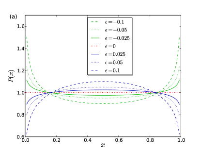
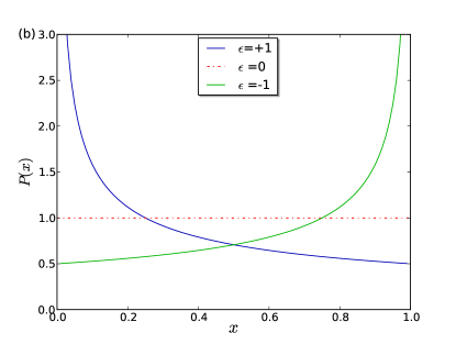
Figure 1: (Color online) Influence of an insufficient posterior on the DIP distribution $P(x)$. The (a) upper [(b) lower] panel shows the effect of calculating $P(x)$ from a posterior with wrong variance [skewness] as described by Eq. (5) [Eq. (7)].

Wrong skewness. Next, we consider the case in which $P(x)$ was calculated from a falsely skewed posterior,

$$P^{\epsilon}(s|d)=\frac{1}{\sqrt{2\pi}\sigma}\exp{\left(-\frac{s^{2}_{d}}{2\sigma^{2}}\right)}\left(1+\text{erf}{\left(\frac{\epsilon s_{d}}{\sqrt{2}\sigma}\right)}\right).$$ (7)

Thus, $x^{\epsilon}$ is given by

$$\begin{split}x^{\epsilon}=&\frac{1}{2}\left[1+\text{erf}{\left(\frac{s_{d}}{\sqrt{2}\sigma}\right)}\right]\\ &-\frac{1}{\pi}\int_{0}^{\epsilon}d\tilde{\epsilon}~{}\frac{\exp{\left(-\frac{1}{2}\left(\frac{s_{d}}{\sigma}\right)^{2}\left(1+\tilde{\epsilon}^{2}\right)\right)}}{1+\tilde{\epsilon}^{2}}\\ =:&\frac{1}{2}\left[1+\text{erf}{\left(\frac{s_{d}}{\sqrt{2}\sigma}\right)}\right]-2T{\left(\frac{s_{d}}{\sigma},\epsilon\right)},\end{split}$$ (8)

where $T{\left(\frac{s_{d}}{\sigma},\epsilon\right)}$ is the Owen’s function Owen (1956), and $\epsilon$ denotes the dimensionless skewness parameter. Now we focus on $|\epsilon|=1$ for simplicity, for which $2T{\left(\frac{s_{d}}{\sigma},\pm 1\right)}=\pm\frac{1}{4}\left(1-\text{erf}^{2}{\left(\frac{s_{d}}{\sqrt{2}\sigma}\right)}\right)$. Applying Eq. (28) yields

$$P(x)=\left\{\begin{array}[]{cc}\left(2\sqrt{x}\right)^{-1}&~{}~{}~{}~{}~{}~{}~{}~{}~{}~{}\text{if}~{}\epsilon=1\\ \left(2\sqrt{1-x}\right)^{-1}&~{}~{}~{}~{}~{}~{}~{}~{}~{}~{}\text{if}~{}\epsilon=-1\end{array}\right..$$ (9)

The effect of an incorrectly skewed posterior is an enhancement of values close to $x=0$ or $x=1$ [Fig. 1(b)] and means that the $68\%$ confidence interval around the expectation value (maximum of the Gaussian PDF) is falsely calculated to be asymmetric. Here, we restricted ourselves to the cases $\epsilon=\pm 1$ due to their analytic treatability. Smaller deviations with $|\epsilon|<1$ will lead to qualitatively similar but less pronounced distortions of the sampled distribution $P(x)$.

Wrong maximum position. In the case in which $P(x)$ was calculated from a posterior whose maximum has a wrong position, we consider

$$\begin{split}P^{\epsilon}(s|d)&=\frac{1}{\sqrt{2\pi}\sigma}\exp{\left(-\frac{(s_{d}-\epsilon)^{2}}{2\sigma^{2}}\right)},\\ x^{\epsilon}&=\frac{1}{2}\left[1+\text{erf}{\left(\frac{s_{d}-\epsilon}{\sqrt{2}\sigma}\right)}\right].\end{split}$$ (10)

Applying again Eq. (28) yields

$$P(x)=\exp{\left(-\frac{1}{2}\left(\frac{\epsilon}{\sigma}\right)^{2}-\sqrt{2}\left(\frac{\epsilon}{\sigma}\right)~{}\text{erf}^{-1}{\left(2x-1\right)}\right)},$$ (11)

with the limit $P(x)\stackrel{{\scriptstyle\epsilon\rightarrow 0}}{{\longrightarrow}}1$. The resulting distribution of $x$ for $\sigma=1$ is shown in Fig. 2. Here, the $x$ abundances near $x=0$ or $x=1$ are enhanced, similarly to the case of incorrect skewness. However, the slope of $P(x)$ at the suppressed end differs significantly from the former case.

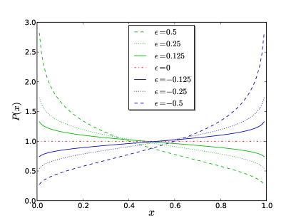
Figure 2: (Color online) Influence of an insufficient posterior on the DIP distribution $P(x)$. The panel is showing the effect of calculating $P(x)$ from a posterior with wrong maximum position as described by Eq. (10).

Wrong normalization. Lastly, we consider the case in which $P(x)$ was calculated from a posterior with wrong normalization,

$$\begin{split}P^{\epsilon}(s|d)&=\frac{1}{\sqrt{2\pi}\sigma(1+\epsilon)}\exp{\left(-\frac{s_{d}^{2}}{2\sigma^{2}}\right)},\\ x^{\epsilon}&=\frac{1}{2(1+\epsilon)}\left[1+\text{erf}{\left(\frac{s_{d}}{\sqrt{2}\sigma}\right)}\right],\end{split}$$ (12)

which yields [Eq. (28)]

$$P(x)=1+\epsilon~{}~{}~{}~{}~{}~{}\text{for}~{}x\in[0,1-\epsilon].$$ (13)

This means the value of $\epsilon$ can be determined precisely from the $x$ interval.

II.2.2 DIP – overview

Table 1 summarizes typical error signatures that can easily be detected by visual inspection of the DIP test.

Table 1: Summary of the DIP test scenarios. The table shows the connection between the numerical (or caused by approximations) error type and the graphical effect.

Graphical effect	Error type
Flat distribution	–
“$\cup$ ($\cap$)shape”	Variance under-(over)estimated
$x=0$ ($x=1$) enhanced,
concave	Too neg. (pos.) skewed
$x=0$ ($x=1$) enhanced,
concave and convex	Too large (low) max. postition
$x$-interval smaller
(greater) than one	Too large (low) normalization

Note that any combination of the errors mentioned in Table 1 could appear, translating into a superposition of the particular graphical effects. An asymmetric “$\cup$ shape”, for instance, where abundances near $x=0$ are slightly enhanced would illustrate an underestimation of the variance combined with a too positive skewness or a too large maximum position. However, in practice often one error dominates. In that case the fitting formulas of Sec. II.B.1 are applicable.

II.3 Numerical example of an insufficient posterior

Next, we demonstrate the effects of insufficient posteriors with a numerical example. For this we generate mock data according to

$$d=s+n,$$ (14)

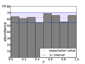
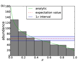
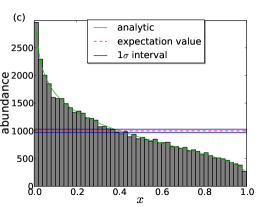
Figure 3: (Color online) Distributions of the numerically calculated $x$-values. The (a) left [(b) middle, (c) right] histogram shows the unnormalized distribution of 500 [500, 50000] $x$-values within eight [eight, fifty] bins as calculated from the posterior with correct [wrong, wrong] maximum position. The standard deviation interval (1$\sigma$) around the expectation value as calculated from Poissonian statistics is also shown.

where $s$ and $n$ are zero-centered Gaussian random numbers with covariance $S=1$ and $N=0.1$, respectively. To reconstruct $s$ optimally from the data we apply a Wiener filter Wiener (1949) on $d$,

$$m=\underbrace{\left(S^{-1}+N^{-1}\right)^{-1}}_{=:D}N^{-1}d.$$ (15)

After that, the posterior for $s$ is given by

$$P(s|d)=\mathcal{G}(s-m,D).$$ (16)

To investigate the accuracy of our implementation we go through the DIP validation procedure. For that purpose we sample $s_{\text{gen}}$ values from the distribution $\mathcal{G}(s,S)$. Next, we generate data according to Eq. (14) and calculate a posterior curve according to Eq. (16). Subsequently, we numerically determine the posterior probability for $s<s_{\text{gen}}$, which is denoted by $x$. Now this procedure is repeated $500$ times to sample $P(x)$.

In order to demonstrate the effect of an insufficient posterior we falsely include a wrong maximum position with $\epsilon=0.15$, i.e. our wrong test posterior is given by

$$P^{\epsilon=0.15}(s|d)=\mathcal{G}(s-m-0.15,D),$$ (17)

and apply the validation procedure once again. Figure 3 shows the distributions of $x$ for the correct and incorrect posterior.

The results are in agreement with the analytical considerations.

II.4 Application to an actual physical problem

An application of the DIP test in precision cosmology and its implications is given in Dorn et al. (2013). There, a new way to calculate the posterior for the local primordial non-Gaussianity parameter $f_{\text{nl}}$ from cosmic microwave background observations is presented and validated via the DIP test. Thereby a numerical problem in the implementation of the posterior could be detected and classified.

III DIP in higher dimensions

Although we have presented the DIP test in one dimension ($s\in\mathds{R}$), this approach can in principle be extended to arbitrary dimensions ($t\in\mathds{R}^{m},~{}m\in\mathds{N}$) by mapping this multidimensional posterior $P(t|d)$ onto one dimension, $s=s(t)\in\mathds{R}$, by the usage of a marginalization, $P(s|d)=\int\mathcal{D}t~{}P(s|t,d)P(t,d)$. Now it is possible to apply the DIP test for the remaining coordinate, $P(s|d)$. Because there are infinitely many ways to perform the mapping, $t\mapsto s=s(t)$, a suite of tests can be constructed to probe $P(t|d)$ in various ways. A combination of these tests then yields a multidimensional posterior test.

In the following two two-dimensional examples should illustrate this.

III.1 Analytical example in two dimensions

The following analytical example should demonstrate the DIP test in higher dimensions. Within this example we choose mappings onto one dimension (parametrized by $\phi$), which are not the most suitable ones to detect an error. We will show, however, that the DIP test is still able to detect and classify an error. For this purpose we assume a correct posterior distribution, given by a two-dimensional Gaussian with zero mean,

$$\begin{split}P&(t|d)=\frac{1}{\sqrt{(2\pi)^{2}}\sigma_{x}\sigma_{y}}\\ \times&\exp\left(-\frac{1}{2}\left(\begin{array}[]{c}t_{x}\\ t_{y}\end{array}\right)^{T}\left(\begin{array}[]{cc}\sigma_{x}^{-2}&0\\ 0&\sigma_{y}^{-2}\end{array}\right)\left(\begin{array}[]{c}t_{x}\\ t_{y}\end{array}\right)\right),\end{split}$$ (18)

and falsely manipulate the variance by setting $\sigma_{x}\rightarrow\sigma_{x}(1+\epsilon)$, i.e., we consider a wrong distribution, $P^{\epsilon}(t|d)$, with too large standard deviation along the $t_{x}$ axis. From now on we set $\sigma_{x}=\sigma_{y}=:\sigma$ for simplicity. Next, we have to map the test distribution, $P^{\epsilon}(t|d)$, onto one dimension to apply the DIP test. One way to do this is to consider the intersection of $P^{\epsilon}(t|d)$ with the hypersurface given by $t_{y}=t_{x}\tan(\phi)$, where $\phi\in[0,2\pi]$ denotes the usual azimuth in the $t_{y}$-$t_{x}$ plane. After this mapping (and choice of a proper normalization) we obtain

$$\begin{split}P_{\text{1d}}(t|d)=&~{}\frac{1}{\sqrt{2\pi}\sigma_{\phi}}~{}\exp\left(-\frac{1}{2}\frac{t_{x}^{2}}{\sigma_{\phi}^{2}}\right),\\ P_{\text{1d}}^{\epsilon}(t|d)=&~{}\frac{1}{\sqrt{2\pi}\sigma_{\phi}^{\epsilon}}~{}\exp\left(-\frac{1}{2}\frac{t_{x}^{2}}{\left(\sigma_{\phi}^{\epsilon}\right)^{2}}\right),\end{split}$$ (19)

with

$$\begin{split}\sigma_{\phi}:=&~{}\frac{\sigma}{\sqrt{1+\tan^{2}(\phi)}},\\ \sigma_{\phi}^{\epsilon}:=&~{}\frac{\sigma}{\sqrt{\frac{1}{(1+\epsilon)^{2}}+\tan^{2}(\phi)}}.\end{split}$$ (20)

The determination of the $\phi$ dependent $P(x)$, $P_{\phi}(x)$, works analogous to the wrong variance section of II.B.1 and yields

$$P_{\phi}(x)=\frac{\sigma_{\phi}^{\epsilon}}{\sigma_{\phi}}\exp\left(-\left[\text{erf}^{-1}{\left(2x-1\right)}\right]^{2}\left[\left(\frac{\sigma_{\phi}^{\epsilon}}{\sigma_{\phi}}\right)^{2}-1\right]\right),$$ (21)

with the limits

$$\begin{split}\frac{\sigma_{\phi}^{\epsilon}}{\sigma_{\phi}}\bigg{|}_{\phi=0,\pi}=&~{}1+\epsilon,\\ \lim_{\phi\rightarrow\frac{\pi}{2},\frac{3\pi}{2}}\left(\frac{\sigma_{\phi}^{\epsilon}}{\sigma_{\phi}}\right)=&~{}1.\end{split}$$ (22)

Figure 4 illustrates this result for an overestimation of the variance, $\epsilon=0.3$, and $\phi\in[0,\frac{\pi}{2}]$. In this case the DIP test shows significant deviations from an accurate posterior within a finite $\phi$ range. That means the DIP test indicates the insufficiency of the posterior even without hitting the exact parameter constellation (here, $\phi=0$). Thus, in this example it is sufficient to perform at most two DIP tests (even though one can construct infinitely many) with $\Delta\phi=\frac{\pi}{2}$ to get an indication of the insufficiency of the posterior.

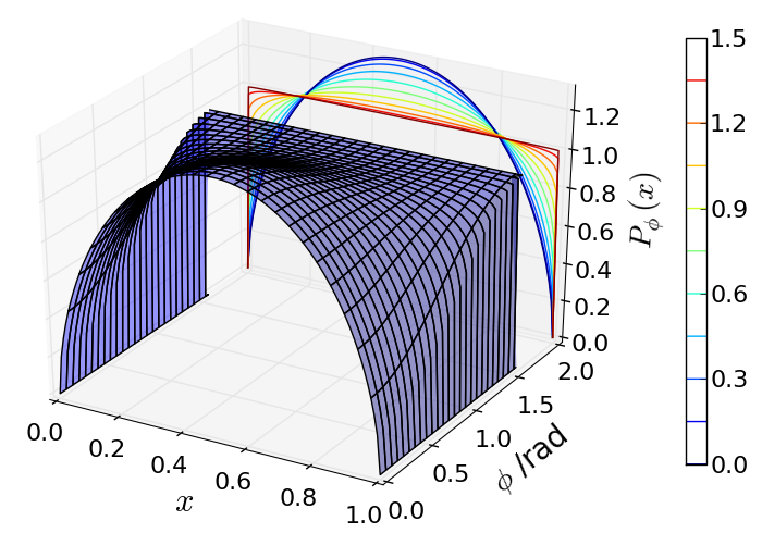
Figure 4: (Color online) DIP test in two dimensions with related contour plot, according to Eq. (21). $\phi$ denotes the azimuth (of the $t_{x}$-$t_{y}$ plane), where the two-dimensional posterior $P^{\epsilon}(s|d)$ intersects with a plane, given by $t_{y}=t_{x}\tan(\phi)$. The DIP distribution of the resulting one-dimensional posterior is denoted by $P_{\phi}(x)$. The labeling of the color bar refers to the $\phi$ coordinate.

III.2 Numerical example of a Bayesian hierarchical model

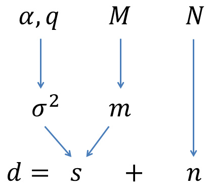
Figure 5: (Color online) Scheme of the Bayesian hierarchical model.

To demonstrate the practical relevance in posterior computation we consider a Bayesian hierarchical model, where the data $d\in\mathds{R}$ are given by $d=s+n$, with $n$ a white Gaussian noise. The signal $s$ itself depends on a mean $m\in\mathds{R}$, drawn from the Gaussian $\mathcal{G}(m,M)$ with related variance $M$ and on a signal variance, $\sigma^{2}\in\mathds{R}$. The signal variance is drawn from an inverse-Gamma distribution,

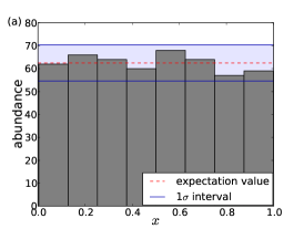
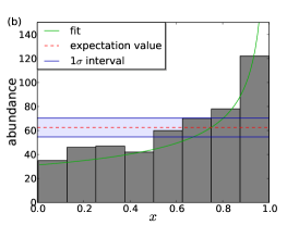
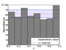
Figure 6: (Color online) Distributions of the numerically calculated $x$ values. The (a) left [(b) middle, (c) right] histogram shows the unnormalized distribution of 500 $x$ values within eight bins as calculated from the $m$- [$m$-, $\sigma^{2}$-] marginalized posterior with correct [wrong, wrong] $\alpha$ parameter. The standard deviation interval (1$\sigma$) around the expectation value as calculated from Poissonian statistics is also shown.

$$\mathcal{I}{\left(\sigma^{2};\alpha,q\right)}:=\frac{q^{\alpha}}{\Gamma(\alpha)}\sigma^{2-\alpha-1}\exp{\left(-\frac{q}{\sigma^{2}}\right)},$$ (23)

with $\Gamma$ the Gamma function and shape parameters $\alpha,~{}q$. Figure 5 illustrates the constituents of the data. Furthermore, we assume the following reasonable relations:

$$\begin{split}P{\left(m,\sigma^{2}\right)}=&~{}\mathcal{G}(m,M)~{}\mathcal{I}{\left(\sigma^{2};\alpha,q\right)},\\ P{\left(s|m,\sigma^{2}\right)}=&~{}\mathcal{G}{\left(s-m,\sigma^{2}\right)},~{}\text{and}\\ P(d|s)=&~{}\mathcal{G}(d-s,N),\end{split}$$ (24)

where $N$ denotes the noise covariance. In this example we want to reconstruct $m$ and $\sigma^{2}$ from given data $d$ (a similar problem is stated in Jaynes and Bretthorst (2003)), i.e. we want to determine the posterior,

$$\begin{split}P&{\left(m,\sigma^{2}|d\right)}\\ =&~{}\frac{1}{\mathcal{N}}~{}\mathcal{G}(m,M)~{}\mathcal{I}{\left(\sigma^{2};\alpha,q\right)}\\ &\times\int ds~{}\mathcal{G}(d-s,N)~{}\mathcal{G}{\left(s-m,\sigma^{2}\right)}\\ =&~{}\frac{\mathcal{G}(m,M)~{}\mathcal{I}{\left(\sigma^{2};\alpha,q\right)}~{}\mathcal{G}{\left(d-m,\sigma^{2}+N\right)}}{\int_{0}^{\infty}d\sigma^{2}~{}\mathcal{I}{\left(\sigma^{2};\alpha,q\right)}~{}\mathcal{G}{\left(d,\sigma^{2}+M+N\right)}},\end{split}$$ (25)

where $\mathcal{N}$ denotes the normalization. In the implementation of Eq. (25) we falsely include an error by setting $\alpha\rightarrow\alpha(1+\epsilon)$ and apply afterwards the DIP test to investigate the accuracy of the posterior, $P^{\epsilon}{\left(m,\sigma^{2}|d\right)}$. For this purpose we have to map the posterior onto one dimension. We choose two natural mappings, given by an $m$- or $\sigma^{2}$ marginalization of the posterior,

$$\begin{split}P{\left(\sigma^{2}|d\right)}=&\int dm~{}P{\left(m,\sigma^{2}|d\right)}\\ =&~{}\frac{1}{\mathcal{N}}~{}\mathcal{G}{\left(d,\sigma^{2}+M+N\right)}~{}\mathcal{I}{\left(\sigma^{2};\alpha,q\right)},\end{split}$$ (26)

or

$$\begin{split}P{\left(m|d\right)}=&\int_{0}^{\infty}d\sigma^{2}~{}P{\left(m,\sigma^{2}|d\right)}\\ =&~{}\frac{1}{\mathcal{N}}~{}\mathcal{G}(m,M)~{}\\ &\times\int_{0}^{\infty}d\sigma^{2}~{}\mathcal{I}{\left(\sigma^{2};\alpha,q\right)}~{}\mathcal{G}{\left(d-m,\sigma^{2}+N\right)}.\end{split}$$ (27)

The results of the DIP test from 500 data realizations for $\alpha=2,~{}q=1,~{}M=1,~{}N=0.1$ and $\epsilon=0.3$ are shown by Fig. 6, where the (a) left histogram shows the accuracy of the posterior implementation for $\epsilon=0$. The (b) middle histogram shows the DIP test for $P^{\epsilon=0.3}{\left(\sigma^{2}|d\right)}$ according to Eq. (26). Here, the wrong implementation of the $\alpha$ parameter transfers into a wrong posterior, whose inaccuracy is mainly dominated by an incorrect, too positive, skewness. The fit illustrates Eq. (9) with $\epsilon=-1$. The (c) right histogram shows the DIP test for $P^{\epsilon=0.3}(m|d)$ according to Eq. (27). In this case the wrong implementation does not transfer into a significant deviation from a uniform distribution, since the mean is almost unattached.

To summarize, the DIP tests shows significant insufficiencies for $P(\sigma^{2}|d)$, even though it might not be the most suitable mapping to detect insufficiencies of the $\alpha$ parameter. For $P(m|d)$ the DIP test cannot detect insufficiencies. However, although one can construct infinitely many mappings onto one dimension, two natural marginalizations of the posterior onto one dimension have been sufficient to reveal the insufficiency of the implementation.

IV Conclusion and outlook

With the help of the introduced DIP test tools of error diagnosis it is possible to detect not only the presence of the inaccuracy but also to get an indication of its nature and the size of impact on the posterior distribution.

Furthermore, it is theoretically possible to do not only a qualitative error diagnosis, but also a quantitative study. One possibility is to consider the intersection of the distribution $P(x)$ of an insufficient posterior with the expectation value, $P(x)=1$, which encodes [in combination with the shape and slope of $P(x)$] the value of $\epsilon$. However, in reality there are combinations of different error types and numerically determined distributions are not as precise as the theoretical ones so that one might want to construct a Bayesian test for this.

We leave the development of fully automated error detection and classification methods for future work. Inspection of the results of the DIP test by eye is already a powerful way to diagnose posterior imperfections, as we show in Dorn et al. (2013).

Appendix A Uniformity of $P(x)$

Proof. We show here analytically that $P(x)=1$ if $\tilde{P}(s|d)=P(s|d)$:

$$\begin{split}P(x)&=\int_{-\infty}^{\infty}ds\int\mathcal{D}d~{}P(x,d,s)\\ &=\int_{-\infty}^{\infty}ds\int\mathcal{D}d~{}P(x|d,s)P(d,s)\\ &=\int_{-\infty}^{\infty}ds\int\mathcal{D}d~{}P(d,s)~{}\delta\left(x-\int_{-\infty}^{s}ds^{\prime}~{}P(s^{\prime}|d)\right)\\ &=\int_{-\infty}^{\infty}ds\int\mathcal{D}d~{}P(d)P(s|d)~{}\delta(x-x_{d}(s)),\end{split}$$ (28)

where $x_{d}(s):=\int_{-\infty}^{s}ds^{\prime}~{}P(s^{\prime}|d)$ and $\int\mathcal{D}d$ denotes a path integral over all possible realizations of $d$. Now we show $P(x)=1$ for $x\in[0,1]$:

$$\begin{split}P&(x)=\partial_{x}\int_{0}^{x}dx^{\prime}P(x^{\prime})\\ &=\partial_{x}\int\mathcal{D}d~{}P(d)\int_{-\infty}^{\infty}ds~{}P(s|d)\underbrace{\int_{0}^{x}dx^{\prime}~{}\delta(x^{\prime}-x_{d}(s))}_{\Theta(x-x_{d}(s))}\\ &=\partial_{x}\int\mathcal{D}d~{}P(d)\int_{-\infty}^{s_{d}(x)}ds~{}P(s|d)\\ &=\partial_{x}\int\mathcal{D}d~{}P(d)\underbrace{x_{d}(s_{d}(x))}_{=x}=\partial_{x}x\int\mathcal{D}d~{}P(d)\\ &=\partial_{x}x=1\end{split}$$ (29)

Here $s_{d}(x)~{}\text{is the inverse of}~{}x_{d}(s)$ and $\Theta$ the Heaviside step function. This inverse exists because $x_{d}(s)$ is strictly monotonous, unless $P(s|d)=0$ exactly for some $s$ range. $\blacksquare$

Appendix B Mapping to a Gaussian

We assume $P(x)$ to be an arbitrary one-dimensional probability distribution with related cumulative distribution, $F(X)=\int_{0}^{X}dx~{}P(x)$, and $\mathcal{G}(x,1)$ to be a one-dimensional Gaussian with related cumulative distribution, $G(X)$.

Here, we prove that $P(y)=\mathcal{G}(y,1)$ if the coordinate transformation is given by $y(x)=G^{-1}{\left(F(x)\right)}$:

$$\begin{split}P(y)dy=&~{}P(x)dx\\ &\Leftrightarrow\\ P(y)=&~{}P(x)\bigg{|}\frac{dx}{dy}\bigg{|}_{x=F^{-1}{\left(G(y)\right)}}\\ =&~{}P{\left(F^{-1}{\left(G(y)\right)}\right)}\frac{\partial F^{-1}{\left(G(y)\right)}}{\partial y}\\ =&~{}P{\left(F^{-1}{\left(G(y)\right)}\right)}\left(\frac{\partial F{\left(F^{-1}{\left(G(y)\right)}\right)}}{\partial y}\right)^{-1}\frac{\partial G(y)}{\partial y}\\ =&~{}\frac{P{\left(F^{-1}{\left(G(y)\right)}\right)}}{P{\left(F^{-1}{\left(G(y)\right)}\right)}}~{}\mathcal{G}(y,1)=\mathcal{G}(y,1)\hskip 28.45274pt\blacksquare\end{split}$$ (30)

References

• Bennett et al. (2012) C. L. Bennett, D. Larson, J. L. Weiland, N. Jarosik, G. Hinshaw, N. Odegard, K. M. Smith, R. S. Hill, B. Gold, M. Halpern, et al., ArXiv e-prints (2012), eprint 1212.5225.
• Planck Collaboration et al. (2013) Planck Collaboration, P. A. R. Ade, N. Aghanim, C. Armitage-Caplan, M. Arnaud, M. Ashdown, F. Atrio-Barandela, J. Aumont, C. Baccigalupi, A. J. Banday, et al., ArXiv e-prints (2013), eprint 1303.5076.
• Geweke (2004) J. Geweke, Journal of the American Statistical Association 99, 799 (2004).
• Cook et al. (2006) S. R. Cook, A. Gelman, and D. B. Rubin, Journal of Computational and Graphical Statistics 15, 675 (2006).
• Bayes (1763) T. Bayes, Phil. Trans. of the Roy. Soc. 53, 370 (1763).
• Dorn et al. (2013) S. Dorn, N. Oppermann, R. Khatri, M. Selig, and T. A. Enßlin, ArXiv e-prints (2013), eprint 1307.3884.
• Casella and Berger (2002) G. Casella and R. Berger, Statistical inference, Duxbury advanced series in statistics and decision sciences (Thomson Learning, 2002), ISBN 9780534243128.
• Owen (1956) D. B. Owen, Ann. Math. Statist. 27, 1075 (1956).
• Wiener (1949) N. Wiener, Extrapolation, Interpolation, and Smoothing of Stationary Time Series (New York: Wiley, 1949), ISBN 9780262730051.
• Jaynes and Bretthorst (2003) E. Jaynes and G. Bretthorst, Probability Theory: The Logic of Science, Chapter 12.4 (Cambridge University Press, 2003), ISBN 9781139435161.