A detailed description of the experimental realisation of quantum illumination protocol

Abstract

In the last years the exploitation of specific properties of quantum states has disclosed the possibility of realising tasks beyond classical limits, creating the new field of quantum technologies [1, 2, 3, 4, 5, 6, 7, 8, 9]. Among them, quantum metrology and imaging aim to improve the sensitivity and/or resolution of measurements exploiting non-classical features such as squeezing and quantum correlations (entanglement and discordant states) [10, 11, 12, 13, 14]. Nevertheless, in most of the realistic scenarios losses and noise are known to nullify the advantage of adopting quantum strategies [15]. In this paper we describe in detail the first experimental realization of quantum illumination protocol aimed to target detection in a noisy environment, that preserves a strong advantage over the classical counterparts even in presence of large amount of noise and losses. The experiment, inspired by the theoretical ideas elaborated in [16, 17, 18, 19] (see also [20, 21]), has been performed exploiting only photon number correlations in twin beams. Thus, for its simplicity it can find widespread use. Even more important by challenging the common believe that real application of quantum technologies is limited by their fragility to noise and losses, it paves the way to their real application.

1 Introduction

In our scheme [22] for target detection a probe beam of a bipartite correlated state may be partially reflected by an object towards a camera, which also receives a thermal field acting as noisy unknown background (thermal bath). Our goal is to investigate the performances of the quantum protocol, in a detection framework in which only photon numbers (i.e. intensities) are measured, with respect to the best classical counterpart, namely a classically-correlated-light based protocol. We show as the use of simple second order correlation measurements already suffices in guaranteeing strong advantages to the quantum protocol. This is a fundamental progress toward a practical realisation respect to some previous similar theoretical proposals [17, 18, 23], stemming from the “quantum illumination” scheme of [16], where the discrimination strategy, based on quantum Chernoff bound [24, 25], was very challenging from an experimental point of view. We realise quantum target detection both by using quantum illumination (QI), specifically twin beams (TWB), and by using classical illumination (CI), e.g. correlated thermal beams (THB), representing the best classical state in the specific detection framework, pointing out unequivocally the experimental advantage of the quantum protocol in mesoscopic regime, independently on the noise level. The realisation of QI protocol, beyond paving the way to future practical application, also provides a significant example of ancilla assisted quantum protocol besides the few previous ones, e.g.[13, 26, 27, 28]. As a first application of quantum illumination to QKD, with a different detection scheme, refer to the recent paper [29].

2 An experimental setup

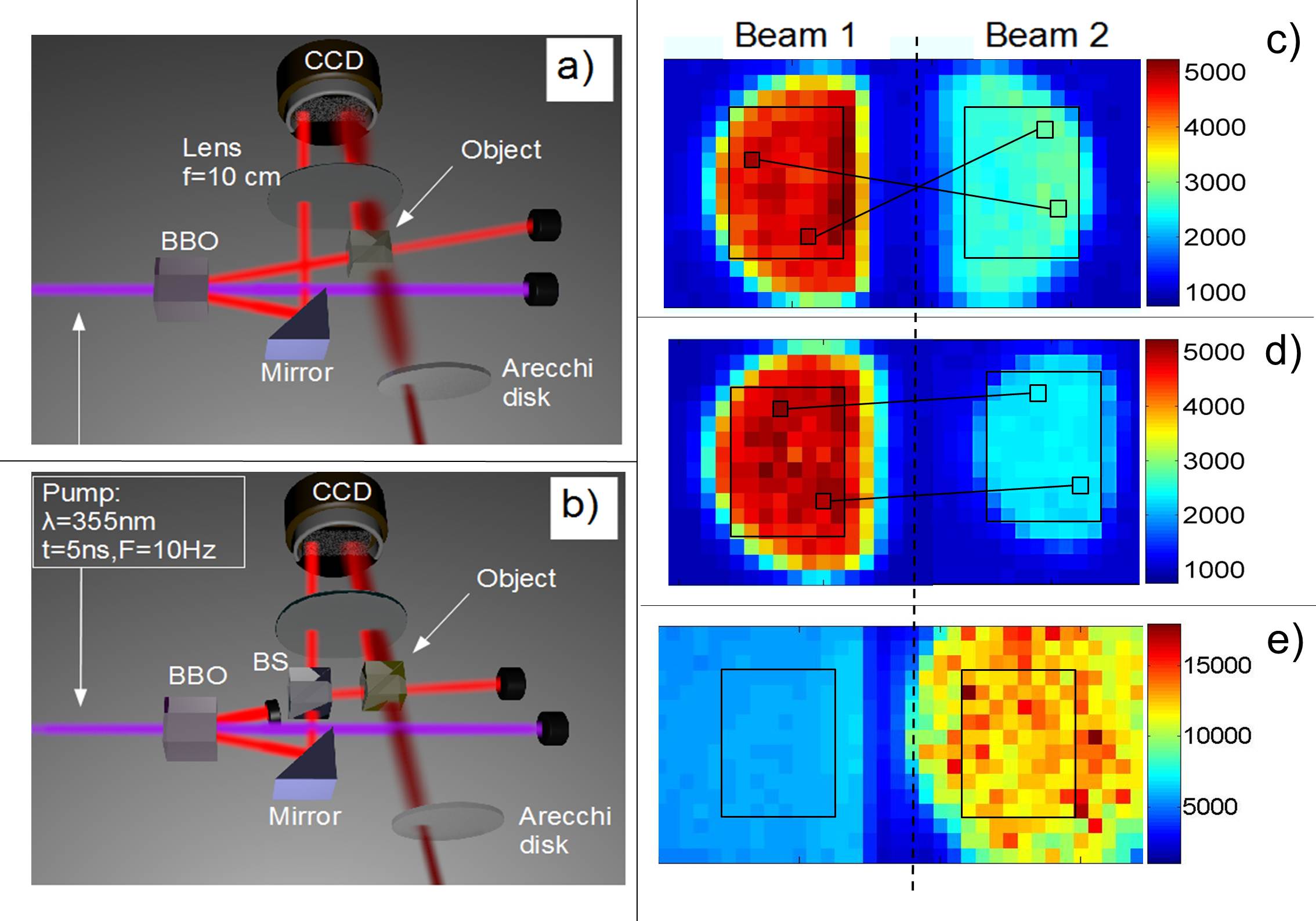
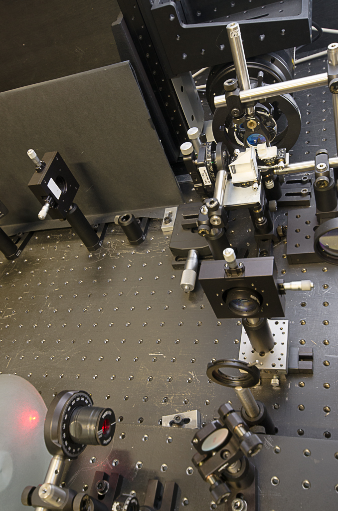
In our setup (Figure 1) correlated photon pairs in orthogonal polarisations are generated in Parametric Down Conversion (PDC) process by pumping a BBO (Beta-Barium-Borate) non-linear crystal with the third harmonic (355 nm) of a Q-switched Nd-Yag laser (repetition rate of 10 Hz, 5 ns pulse width) after spatial filtering. The correlated emissions are then addressed to a high quantum efficiency (about 80 % at 710 nm) CCD camera ($N_{\rm pix}=80$ pixels of size $A_{\rm pix}=(480~{}\mu\hbox{m})^{2}$). The exposure time of the camera is set to collect in a single image the emission generated by a single laser shot. For QI protocol (Figure 1a) after the BBO crystal, where TWB are generated, one of the beam (the “ancilla”) is reflected towards the detection system. The correlated beam is partially detected, together with the thermal field from the Arecchi’s disk, when the object (actually a beam splitter) is present, otherwise it is lost (not showed). Low-pass filter (95 % of transmission at 710nm) and UV-reflecting mirror are used to minimize the background noise while maintaining low losses. A lens, placed at the focal length from the crystal and the CCD camera, realizes the Fourier transform of the field at the output face of the crystal. The PDC light is then combined at the CCD with a thermal background produced by scattering a laser beam on an Arecchi’s rotating ground glass. When the object is removed, only the thermal bath reaches the detector. In order to implement CI protocol (Figure 1b), the TWB are substituted with classical correlated beams. These are obtained by splitting a multi-thermal beam (single arm of PDC) and by setting the pump intensity to ensure equivalent intensity, time and spatial coherence properties for the quantum and the classical sources.

We note that traveling wave PDC generates a spatially multimode emission in the far field, where each mode corresponds to the transverse component of a specific wavevector. Each pair of correlated modes, corresponding to opposite transverse component of the wavevector with respect to the pump direction, are found in symmetric positions [30]. Thus, we choose two correlated regions of interests (ROIs) on the CCD array (showed in Figure 1 c-d-e). The proper sizing of the pixels and the centering of the 2-dimensional array with sub-mode precision, allows to maximize the collection of the correlated photons for each pair of pixels and at the same time to minimize the possible presence of uncorrelated ones [31, 32]. In our experiment, the correlation in the photon number, even at the quantum level for QI, is realized independently for each pair of symmetrical (translated) pixels that belong to the ROIs of the TWB (THB). Therefore, a single image is enough to evaluate correlation parameters, like covariance, averaging over the $N_{\rm pix}$ pairs. Albeit not strictly necessary, this is practically effective because reduces the measurement time (less images are needed) and avoids to deal with the power instability of the pump laser from pulse to pulse, which is very destructive in this kind of application [33]. The number of spatio-temporal modes collected is estimated to be $M=9\cdot 10^{4}$ by fitting a multithermal statistics. The average number of PDC photon per mode is $\mu=0.075$. We measured separately the size of the spatial mode, as the FWHM of the correlation function between the two beams, $A_{\rm corr}=(120\pm 20\mu\hbox{m})^{2}$. Thus, the number of spatial modes is about $M_{\rm sp}=A_{\rm pix}/A_{\rm corr}=16\pm 5$ and the number of temporal modes $M_{\rm t}=M/M_{\rm sp}=(6\pm 2)\cdot 10^{3}$, the last one being consistent with the ratio between the pump pulse duration and the expected PDC coherence time, i.e. 1 ps.

3 The model of the measurement

In our approach, the ability to distinguish the presence/absence of the object depends on the possibility of distinguishing between the two corresponding values of covariance $\Delta_{1,2}$, evaluated experimentally as

$$\Delta_{1,2}=E[N_{1}N_{2}]-E[N_{1}]E[N_{2}],$$ (1)

where the quantity $E[X]=\frac{1}{\mathcal{K}}\sum^{\mathcal{K}}_{k=1}X^{(k)}$ represents the average over the set of $\mathcal{K}$ realizations corresponding in our experiment to the pixels of the ROI, i.e. $\mathcal{K}=N_{\rm pix}$. Therefore, each image provides a determination of the covariance. Then we define the signal to noise ratio (SNR) of counting base QI protocol as the ratio of the mean “contrast” to its standard deviation (mean fluctuation):

$$f_{\rm SNR}\equiv\frac{\left|\left\langle\Delta_{1,2}^{\rm(in)}-\Delta_{1,2}^{\rm(out)}\right\rangle\right|}{\sqrt{\left\langle\delta^{2}\left(\Delta_{1,2}^{\rm(in)}\right)\right\rangle+\left\langle\delta^{2}\left(\Delta_{1,2}^{\rm(out)}\right)\right\rangle}},$$ (2)

where “in” and “out” refer to the presence and absence of the object, respectively and $\langle\cdots\rangle$ is the quantum expectation value. From Eq. (1) follows that $\langle\Delta_{1,2}\rangle=(1-\mathcal{K}^{-1})\langle\delta N_{1}\delta N_{2}\rangle$ and, for $\mathcal{K}>>1$, $\langle\delta^{2}\Delta_{1,2}\rangle\simeq\langle\delta^{2}[\delta N_{1}\delta N_{2}]\rangle/\mathcal{K}$. These expressions allow calculating $f_{\rm SNR}$ theoretically. In particular the denominator can be calculated as

$$\mathcal{K}\left\langle\delta^{2}\Delta_{1,2}\right\rangle\simeq\left\langle\delta^{2}(\delta N_{1}\delta N_{2})\right\rangle\equiv\left\langle\left(\delta N_{1}\delta N_{2}\right)^{2}\right\rangle-\left\langle\delta N_{1}\delta N_{2}\right\rangle^{2}.$$ (3)

By replacing $\delta N_{2}\mapsto\delta N^{(in)}_{2}+\delta N_{b}$ where $N^{(in)}_{2}$ is the number of detected photons that has been reflected by the target, and $N_{b}$ is the uncorrelated background, the right hand side of (3) can be rewritten as

$$\mathcal{K}\langle\delta^{2}\Delta_{1,2}\rangle \simeq \left\langle\left(\delta N_{1}\delta N^{(in)}_{2}+\delta N_{1}\delta N_{b}\right)^{2}\right\rangle-\left\langle\delta N_{1}\delta N^{(in)}_{2}+\delta N_{1}\delta N_{b}\right\rangle^{2}$$

$$= \left\langle\left(\delta N_{1}\delta N^{(in)}_{2}\right)^{2}\right\rangle-\left\langle\delta N_{1}\delta N^{(in)}_{2}\right\rangle^{2}+\left\langle\delta^{2}N_{1}\right\rangle\left\langle\delta^{2}N_{b}\right\rangle$$

$$= \left\langle\delta^{2}(\delta N_{1}\delta N^{(in)}_{2})\right\rangle+\left\langle\delta^{2}N_{1}\right\rangle\left\langle\delta^{2}N_{b}\right\rangle,$$

where we used the statistical independence of $N_{b}$ and the fact that $\langle\delta N_{b}\rangle=0$. It is clear that in the absence of the target (situation labeled with the superscript ”out”), $N^{(in)}_{2}=0$, thus $\langle\delta^{2}\Delta^{(out)}_{1,2}\rangle=\left\langle\delta^{2}N_{1}\right\rangle\left\langle\delta^{2}N_{b}\right\rangle$, since nothing is reflected to the detector. However, if the the background fluctuations $\left\langle\delta^{2}N_{b}\right\rangle$ is the largest contribution to the noise, also when the target is present (indicated with superscript ”in”) we can write $\langle\delta^{2}\Delta^{(in)}_{1,2}\rangle\simeq\left\langle\delta^{2}N_{1}\right\rangle\left\langle\delta^{2}N_{b}\right\rangle$. Under this assumption representing a realistic situation of a very noisy environment, the SNR becomes

$$f_{\rm SNR}\simeq\frac{\langle\delta N_{1}\delta N_{2}\rangle}{\sqrt{2\left\langle\delta^{2}N_{1}\right\rangle\left\langle\delta^{2}N_{b}\right\rangle}}.$$ (5)

We underline that (5) holds for a dominant background, irrespective of its statistics (e.g. multi-thermal or Poissonian).

In our experiment we consider background with multi-thermal statistics. For a generic multi-thermal statistics with number of spatiotemporal modes $M$, mean photon number number per mode $\mu$, the total number of detected photons is $\left\langle N\right\rangle=M\eta\mu$ and the mean squared fluctuation is $\left\langle\delta^{2}N\right\rangle=M\eta\mu(1+\eta\mu)=\left\langle N\right\rangle\left(1+\left\langle N\right\rangle/M\right)$ [see for example [34], where $\eta$ is the detection efficiency.

Thus, the amount of noise introduced by the background can be increased by boosting its total number of photons $\left\langle N_{b}\right\rangle$ or by varying the number of modes $M_{b}$.

Moreover, both TWB and correlated THB present locally the same multi-thermal statistics, but with a number of spatiotemporal modes $M=9\cdot 10^{4}$ much larger than the one used for the background beam ($M_{b}=57$ in one case and, $M_{b}=1.3\cdot 10^{3}$ in the other). This contributes to make the condition of preponderant background effective in our realization, even for a relatively small value of $N_{b}$.

However, we point out that all the theoretical curves reported in all the Figures are evaluated by the exact analytical calculation of the four order (in the number of photons) quantum expectation values appearing on the right hand side of (3), even if the whole expressions are far more complex than the ones obtained with the assumption of preponderant background.

Starting from (5) and considering the same local resources for classical and quantum illumination beams (in particular the same local variance $\left\langle\delta^{2}N_{i}\right\rangle_{CI}=\left\langle\delta^{2}N_{i}\right\rangle_{QI}$ ($i=1,2$)) the enhancement of the quantum protocol can be easily obtained as

$$R=\frac{f^{(QI)}_{\rm SNR}}{f^{(CI)}_{\rm SNR}}\approx\frac{\langle\delta N_{1}\delta N_{2}\rangle_{QI}}{\langle\delta N_{1}\delta N_{2}\rangle_{CI}}=\frac{\varepsilon^{(QI)}}{\varepsilon^{(CI)}}.$$ (6)

with $\varepsilon=\langle:\delta N_{1}\delta N_{2}:\rangle~{}/~{}\sqrt{\langle:\delta^{2}N_{1}:\rangle\langle:\delta^{2}N_{2}:\rangle}$ being the generalized Cauchy-Schwarz parameter, where $\langle:~{}:\rangle$ is the normally ordered quantum expectation value. This parameter is interesting since it does not depends on the losses and it quantifies non-classicality being $\varepsilon\leq 1$ for classical state of light (with positive $P$-function). The covariance of two correlated beams obtained by splitting a single thermal beam is $\langle\delta N_{1}\delta N_{2}\rangle_{TH}=M\eta_{1}\eta_{2}\mu_{TH}^{2}$, while the one of TWB is $\langle\delta N_{1}\delta N_{2}\rangle_{TW}=M\eta_{1}\eta_{2}\mu_{TW}(1+\mu_{TW})$ (see for example [35]). By using this relation with the assumption of the same local resources, $\mu_{TH}=\mu_{TW}=\mu$ we can derive explicitly $R\approx(1+\mu)/\mu$, which is insensitive to the amount of noise and loss. On the other side the generalized Cauchy-Schwarz parameter for a split thermal beam is $\varepsilon_{0}^{(CI)}=1$, where the subscript ”$0$” stands for ”in absence of background”, as it can be easily derived from the equations of covariance and single beam fluctuations used previously. Therefore the comparison with split thermal beams represents the comparison with the ”best” classical case.

4 The results

First of all we evaluate the noise reduction factor (NRF) defined as [13, 32, 36, 37]:

$$\sigma\equiv\frac{\left\langle\delta^{2}(N_{1}-N_{2})\right\rangle}{\left\langle N_{1}+N_{2}\right\rangle},$$ (7)

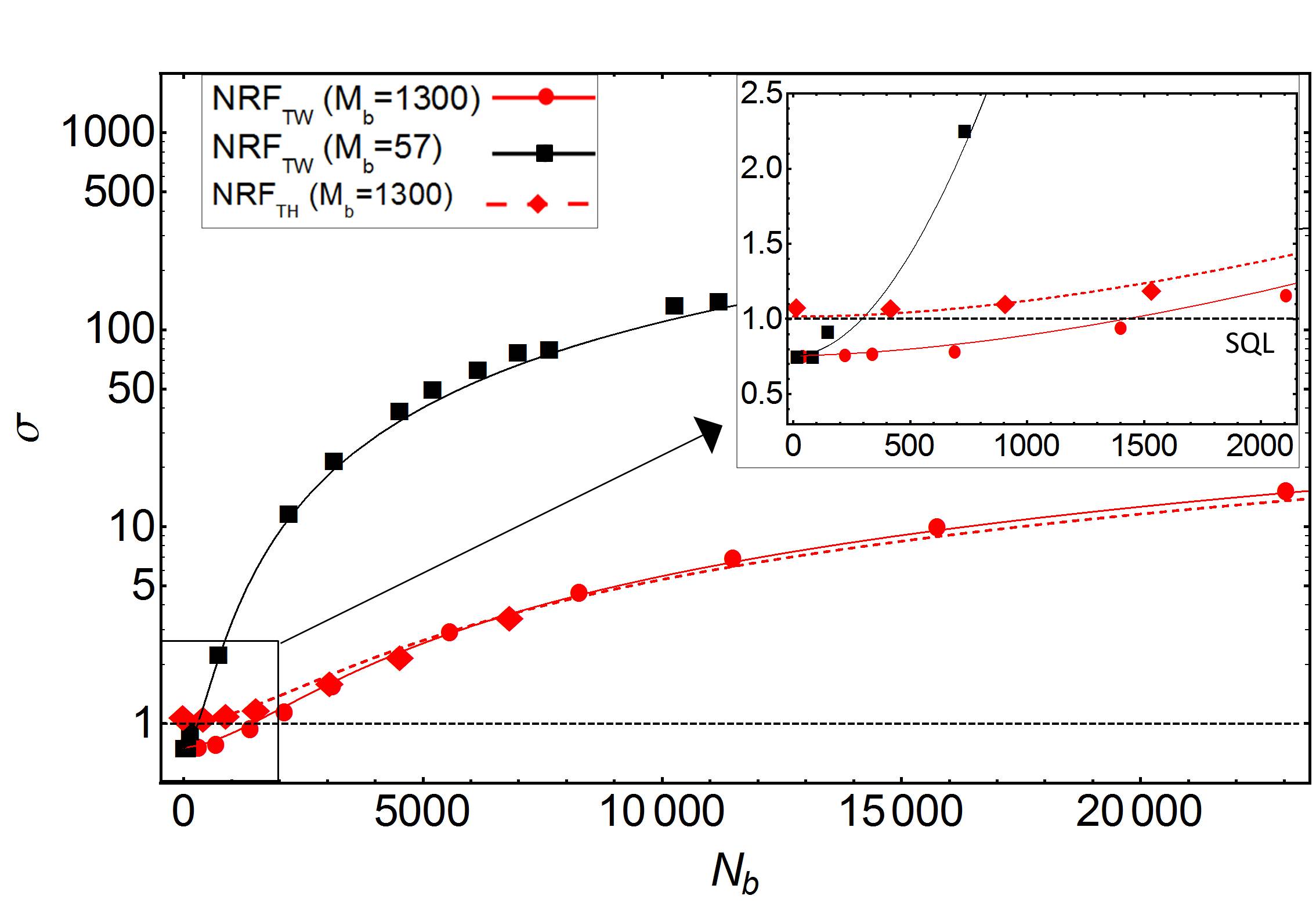
where $\langle N_{i}\rangle$ is the mean value, and $\delta^{2}N_{i}=(N_{i}-\langle N_{i}\rangle)^{2}$ is the fluctuation of the photon number $N_{i}$, $i=1,2$, detected by correlated pixels. It represents the noise of the photon number difference normalized to the shot noise level (SNL) or standard quantum limit (SQL) [32]. For classical states $\sigma\geq 1$, while it is always smaller than 1 for TWB. In particular, when the thermal bath is off, we have $\sigma_{0}=1-\overline{\eta}+(\eta_{1}-\eta_{2})^{2}\left(1/2+\mu\right)/(2\overline{\eta})$, with $\overline{\eta}=(\eta_{1}+\eta_{2})/2$, and $\eta_{i}$ is the overall detection efficiency of beam $i=1,2$[33, 32]. It includes all the transmission-detection losses, thus $\eta_{1}=2\eta_{2}$ due to the presence of the half reflecting object in the path of the second beam. In Figure 2 we report the measured NRF and the theoretical prediction. From the inset one can observe that the NRF is actually in the quantum regime ($\sigma<1$) for small values of the thermal bath, and in absence of it we obtain $\sigma_{0}=0.76$ corresponding to $\eta_{1}=0.4$. While, as soon as the contribution of the bath to the fluctuation of $N_{2}$ becomes dominant, NRF increases quite fast well above the classical threshold. As expected from the multi-thermal character of the bath, the number of modes $M_{b}$ determines the noise level introduced, and it can be tuned easily according to the spin velocity of the ground-glass disk and/or the acquisition time. We also note that, for THB, the NRF is always in the classical regime.

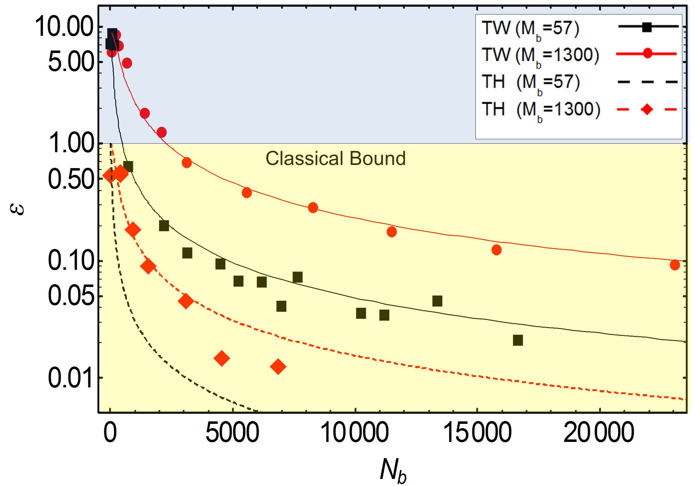
As a second figure of merit, more appropriate for quantifying the quantum resources exploited by our QI strategy we consider the generalized Cauchy-Schwarz parameter $\varepsilon$ introduced in Sec. 3. In Figure 2 we report the measured $\varepsilon$ and the theoretical prediction. One observes that for TWB $\varepsilon^{(QI)}$ is actually in the quantum regime ($\varepsilon^{(QI)}>1$) for small values of the thermal background $\langle N_{b}\rangle$ ($\varepsilon^{(QI)}_{0}\simeq 10$ when $\langle N_{b}\rangle=0$). Also here, $\varepsilon^{(QI)}$ decreases quite fast, well below the classical threshold with the intensity of the background. As expected, for THB $\varepsilon^{(CI)}$ is always in the classical regime(being one for $\langle N_{b}\rangle=0$).

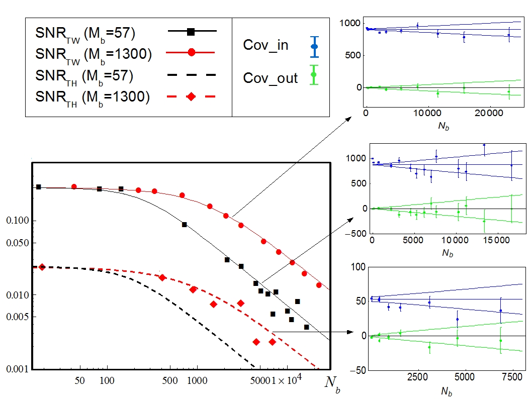
In Figure 3, the $f_{\rm SNR}/\sqrt{\mathcal{K}}$ is compared with the experimental data, where the estimation of quantum mean values of (2) are obtained by performing averages of $\Delta_{1,2}^{\rm(in/out)}$ over a set of $N_{\rm img}$ acquired images. While the SNR unavoidably decreases with the added noise for both QI and CI, the ratio between them is almost constant ($R\gtrsim 10$) regardless the value of $N_{b}$, in agreement with the results of Sec. 3. In turn, the measurement time, i.e., the number of repetitions $N_{\rm img}$ needed for discriminating the presence/absence of the target, is dramatically reduced (for instance, to achieve $f_{\rm SNR}=1$, $N_{\rm img}$ is 100 times smaller when quantum correlations are exploited). Furthermore, Figure 3 shows that the mean value of the covariance does not depend on the quantity of environmental noise, because, as expected, only the correlated components survives to this operation. However, the added noise influences drastically the uncertainty on the measurement for a certain fixed number of images $N_{\rm img}$ and thus the ability to assert the presence of the object.

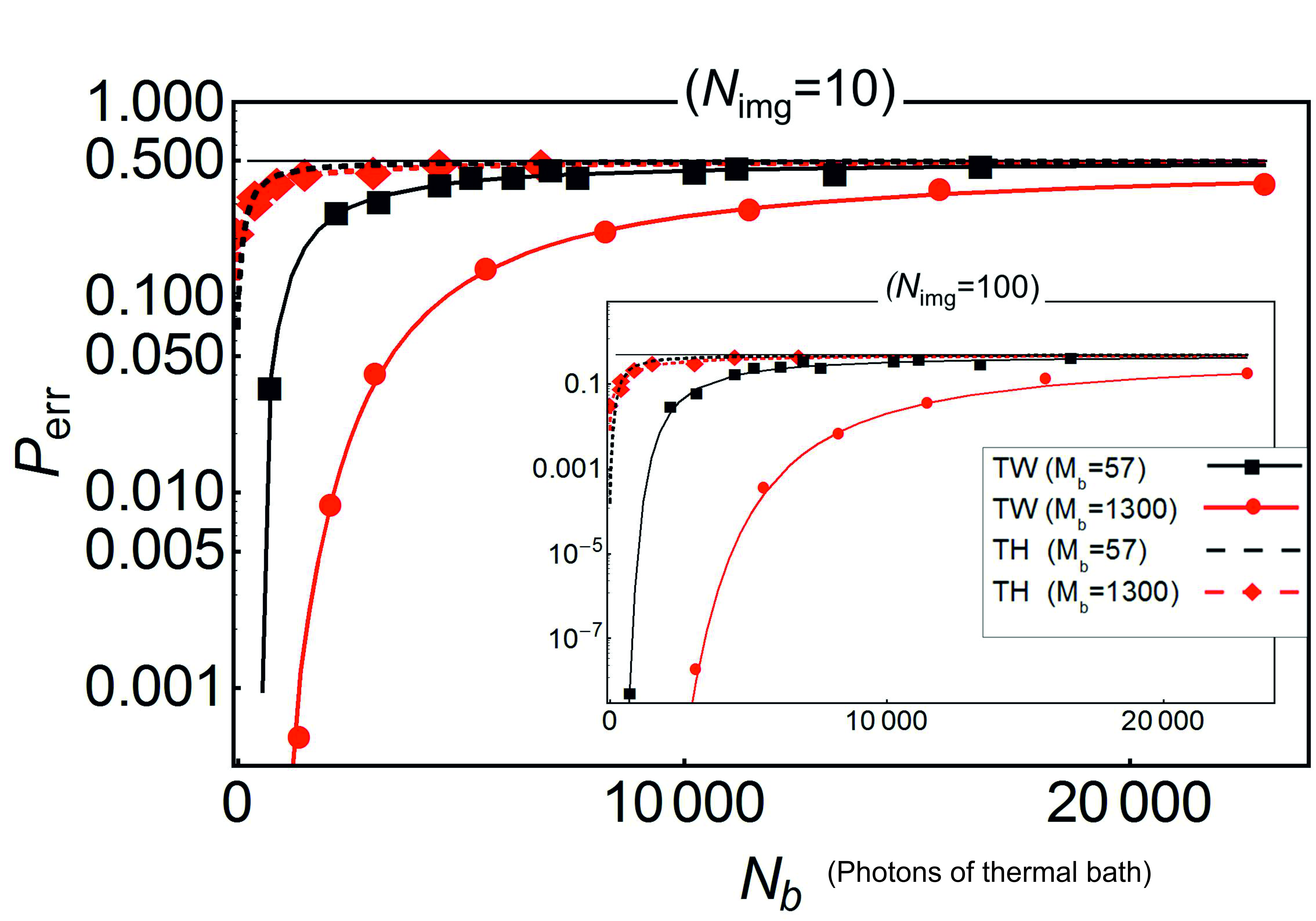
In order to show that the quantum strategy outperforms the classical one, in Figure 4 we report the error probability in the discrimination, $P_{\mathrm{err}}$, versus the number of photons of the thermal bath $N_{b}$. The statement on the presence/absence of the object is performed on the basis of the covariance value obtained for a fixed number of images $N_{\rm img}=10$. Thus, $P_{\mathrm{err}}$ is estimated fixing the threshold value of the covariance that minimizes the error probability itself. Figure 4 shows a remarkable agreement between the theoretical predictions (lines) and the experimental data (symbols), both for QI and CI strategy. Furthermore, the $P_{\mathrm{err}}$ in the case of QI is several orders of magnitude below the CI one and, in terms of background photons, the same value of the error probability is reached for a value of $N_{b}$ at least 10 times larger than in the QI case.

5 Conclusions

We have described in detail the model and the experiment addressed to quantum enhancement in detecting a target in a thermal radiation background in a relevant and realistic measurement scenario. Our system shows quantum correlation with no external noise ($\sigma=0.76$) even in the presence of the losses introduced by the only partially reflective target. Remarkably, even after the transition to the classical regime ($\sigma\gg 1$), the scheme preserves the same strong advantage with respect its natural classical counterpart based on classically correlated beams, as also suggested in [17]. This apparent contradiction is explained by considering that quantum correlations actually survive unchanged up to the detector, where they are simply added to a independent noisy background. Moreover the quantum resources and the quantum enhancement achieved by the protocol can be precisely quantified by the generalized Cauchy-Schwarz parameter that is only related to the source properties $\varepsilon$.

Unlike other quantum enhanced measurement protocols, based on the experimental estimation of the first-moments of the photon number distribution, our scheme, which is based on the measurement of the second order momenta, is impressively robust against losses. This derives from the fact that it does not require high level of two-mode squeezing ($\sigma_{0}=0.76$ in our experiment). For instance the quantum imaging protocol [13], where the signal is given by $\langle N_{1}-N_{2}\rangle$, provides a maximum improving factor of $1/\sqrt{\sigma_{0}}$ over classical techniques, that would correspond to 1.14 in our working condition in the absence of thermal background. Also in exemplar quantum enhanced schemes, such as detection of small beam displacement [11] and phase estimation by interferometry [14], it is well known that losses and noise can rapidly decrease the advantage of using quantum light [15], and typically high level of squeezing is necessary. This enforced inside the generic scientific community the common belief that the advantages of entangled and quantum state are hardly applicable in a real context, and they will remain limited to proofs of principle experiments in highly controlled laboratories, and/or to mere academic discussions. Our work challanges this belief by demonstrating an advantage of orders of magnitude respect to CI protocol, independently on the amount of thermal noise and using devices available nowadays. In summary, we believe that the photon counting based QI protocol has a huge potentiality to foster the exploitation of quantum light based technologies in real lossy and noisy environment.

The research leading to these results has received funding from the EU FP7 under grant agreement n. 308803 (BRISQ2), Fondazione SanPaolo and MIUR (FIRB “LiCHIS” - RBFR10YQ3H, Progetto Premiale “Oltre i limiti classici di misura”).

References

Figure 1: Experimental setup. a) Quantum illumination: b) Classical illumination c) Detected TWB, in the presence of the object, without thermal bath. The region of interest is selected by an interference filter centered around the degeneracy wavelength (710 nm) and bandwidth of 10 nm. After selection the filter is removed. d) Detected field for split thermal beams in the presence of the object, without thermal bath. e) A typical frame used for the measurement, where the interference filter has been removed and a strong thermal bath has been added on the object branch. The color scales on the right correspond to the number of photons per pixel. On the right hand there is the photo of the set-up.

Figure 2: Up, NRF in the case of TWB, NRF_TW, and of the correlated thermal beams, NRF_TH, as a function of the average number of background photons $N_{b}$ for $M_{b}=57$ (black series) and $M_{b}=1300$ (red). The lines represent the theoretical prediction for $\eta_{1}=2\eta_{2}=0.4$ and $\mu=0.075$ (the last estimated independently). For $N_{b}=0$, NRF_TW is $\sigma=0.761\pm 0.006$. Statistical uncertainty bars are too small for being visible. Bottom, generalized Cauchy-Schwarz parameter $\varepsilon$ in the case of twin beams, $\varepsilon^{(\rm TW)}$, and of the correlated thermal beams, $\varepsilon^{(\rm TH)}$, as a function of the average number of background photons $N_{b}$ for a number of background modes $M_{b}=57$ (black series) and $M_{b}=1300$ (red). The lines represent the theoretical prediction at $\mu=0.075$ (the last estimated independently).

Figure 3: SNR versus $N_{b}$ normalized by the square root of number of realization. The red (black) markers refer to $M_{b}=1300$ ($M_{b}=57$) and the solid (dashed) theoretical curve corresponds to quantum (classical) illuminating beams. The lowest curve of the classical protocol has not been compared with the experimental data because the SNR is so low that a very large number of images (out of the possibility of the actual setup) is required to have reliable points. The insets on the left present the covariance in the presence, $\Delta_{1,2}^{\rm(in)}$ (blue), or absence, $\Delta_{1,2}^{\rm(out)}$ (green), of the target. a) and b) refer to QI and CI, respectively, for the same number of bath modes $M_{b}=1300$; c) refers to QI with a a lower number of modes, $M_{b}=57$. Uncertainty bars represent the uncertainty on the mean values of the covariance obtained averaging over the $N_{\rm img}$ images (from the top to bottom: $N_{\rm img}=2000,6000$ and $4000$). Horizontal lines are the theoretical values $\langle\Delta_{1,2}^{\rm(in/out)}\rangle$, while the uncertainty bars should be compared with the gap between the dashed lines, corresponding to the theoretically evaluated $\langle\delta^{2}\Delta_{1,2}^{\rm(in/out)}\rangle/\sqrt{N_{\rm img}}$.

Figure 4: Error probability $P_{\rm err}$ of the target detection versus the total number of photons of the thermal bath $N_{b}$ evaluated with $N_{\rm img}=10$ ($N_{\rm img}=100$ in the inset). The black squares and red circles are the data for QI with $M_{b}=57$ and $M_{b}=1300$, respectively, while red diamonds referes to the data for the CI with $M_{b}=1300$. The curves are the corresponding theoretical predictions.

References

- [1] Bouwmeester D, Pan J W, Mattle K, Eibl M, Weinfurter H and Zeilinger A 1997 et al. Nature 390 575
- [2] Ursin R, Jennewein T, Aspelmeyer M, Kaltenbaek R, Lindenthal M, Walther P and Zeilinger A 2004 Nature 430 849
- [3] Boschi D, Branca S, De Martini F, Hardy L and Popescu S 1998 Phys. Rev. Lett. 80 1121
- [4] O’Brien J L 2007 Science 318 1567
- [5] Yao X C et al 2012 Nature 482 489
- [6] Yamamoto T, Koashi M, Özdemir S K and Imoto N 2003 Nature 421 343
- [7] Pan J W, Simon C, Brukner C and Zeilinger A 2001 Nature 410 1067
- [8] Pan J W, Gasparoni S, Ursin R, Weihs G and Zeilinger A 2003 Nature 417, 4174
- [9] Ruo Berchera I, Degiovanni I P, Olivares S and Genovese M 2013 Phys. Rev. Lett. 110 213601
- [10] Kolobov M I 2007 Quantum Imaging (New York: Springer)
- [11] Treps N, Grosse N, Bowen W P, Fabre C, Bachor H A and Lam P K 2003 Science 301 5635 940
- [12] Boyer V, Marino A M, Pooser R C and Lett P D 2008 Science 321 544
- [13] Brida G, Genovese M and Ruo Berchera I 2010 Nature Photonics 4 227
- [14] Giovannetti V, Lloyd S and Maccone L 2011 Nat. Phot. 5 222-229
- [15] Thomas-Peter N, Smith B J, Datta A, Zhang L, Dorner U and Walmsley I A 2011 Phys. Rev. Lett. 107 113603
- [16] Lloyd S 2008 Science 321 1463
- [17] Tan S-H, Erkmen B I, Giovannetti V, Guha S, Lloyd S, Maccone L, Pirandola S and Shapiro J H 2008 Phys. Rev. Lett. 101 253601
- [18] Shapiro J H and Lloyd S 2009 New Journ. of Phys. 11 063045
- [19] Guha S and Erkmen B I 2009 Phys. Rev. A 80, 052310
- [20] Sacchi M F 2005 Phys. Rev. A 71 062340
- [21] Sacchi M F 2005 Phys. Rev. A 72 014305
- [22] Lopaeva E D, Ruo Berchera I, Degiovanni I P, Olivares S, Brida G and Genovese M 2013 Phys. Rev. Lett. 110 153603
- [23] Shapiro J 2009 Phys. Rev. A 80 022320
- [24] Audenaert K M R, Calsamiglia J, Muñoz-Tapia R, Bagan E, Masanes L, Acín A and Verstraete F 2007 Phys. Rev. Lett. 98 160501
- [25] Calsamiglia J, Muñoz-Tapia R, Masanes L, Acin A and Bagan E 2008 Phys. Rev. A 77 032311
- [26] Brida G, Ciavarella L, Degiovanni I P, Genovese M, Migdall A, Mingolla M G, Paris M G A, Piacentini F and Polyakov S V 2012 Phys. Rev. Lett. 108 253601
- [27] Takahashi H, Wakui K, Suzuki S, Takeoka M, Hayasaka K, Furusawa A and Sasaki M 2008 Phys. Rev. Lett. 101 233605
- [28] Altepeter J B, Branning D, Jeffrey E, Wei T C, Kwiat P G, Thew R J, O’Brien J L, Nielsen M A and White A G 2003 Phys. Rev. Lett. 90 193601
- [29] Zhang Z, Tengner M, Zhong T, Wong F N C and Shapiro J H 2013 Phys. Rev. Lett. accepted for publication
- [30] Brambilla E, Gatti A, Bache M and Lugiato L A 2004 Phys. Rev. A 69 023802
- [31] Pinel O, Fade J, Braun D, Jian P, Treps N and Fabre C 2012 Phys. Rev. A 85 010101(R)
- [32] Brida G, Genovese M, Meda A and Ruo Berchera I 2011 Phys. Rev. A 83 033811
- [33] Brida G, Degiovanni I P, Genovese M, Rastello M L and Ruo Berchera I 2010 Opt. Exp. 18 20572
- [34] Mandel L and Wolf E 1995 Optical Coherence and Quantum Optics (Cambridge University Press)
- [35] Brida G, Chekhova M V, Fornaro G A, Genovese M, Lopaeva E D and Ruo Berchera I 2011 Phys. Rev. A 83 063807
- [36] Bondani M, Allevi A, Zambra G, Paris M G A and Andreoni A 2007 Phys. Rev. A 76 013833
- [37] Iskhakov T, Chekhova M V and Leuchs G 2009 Phys. Rev. Lett. 102 183602