On the instabilities of the Walker propagating domain wall solution

Abstract

A powerful mathematical method for front instability analysis that was recently developed in the field of nonlinear dynamics is applied to the 1+1 (spatial and time) dimensional Landau-Lifshitz-Gilbert (LLG) equation. From the essential spectrum of the LLG equation, it is shown that the famous Walker rigid body propagating domain wall (DW) is not stable against the spin wave emission. In the low field region only stern spin waves are emitted while both stern and bow waves are generated under high fields. By using the properties of the absolute spectrum of the LLG equation, it is concluded that in a high enough field, but below the Walker breakdown field, the Walker solution could be convective/absolute unstable if the transverse magnetic anisotropy is larger than a critical value, corresponding to a significant modification of the DW profile and DW propagating speed. Since the Walker solution of 1+1 dimensional LLG equation can be realized in experiments, our results could be also used to test the mathematical method in a controlled manner.

I I. INTRODUCTION

The past century witnessed the quantum leap of the semiconductor industries which gave birth to the computer science and information technology. We are now in an era in which information keeps being generated at a skyrocketing pace such that the net volume of information produced per day might be comparable to that accumulated after years one century ago. As an important participant, magnetic data recording now has assumed the major task of information documentation, through video tapes, hard disks, etc. In order to cope with the exponentially growing information volume, the need to develop data storage devices with higher capacity and faster read/write operation speed is demanded. This intrigue the development of spintronics-the pursuit to employ, in addition to the charge of electrons, their spin properties into applications. As one major branch, magnetic domain wall (DW) propagation along nanowires has attracted considerable attention in recent years due to its potential in achieving, for instance, high-intensity information storage, nonvolatile random access memory and DW logic circuit [1, 2, 3, 4, 5, 6, 7].

It has already been known for almost 40 years that the 1+1 (spatial and time) dimensional Landau-Lifshitz-Gilbert (LLG) equation [8], which universally governs magnetization dynamics, admits a well-known exact Walker propagating DW solution for a biaxial nanowire. It predicts that, in the presence of an external magnetic field, the DW subjects to a rigid-body translational motion which is valid when the magnetic field is in a proper regime. Despite its attractive simplicity and elegance, and the fact that this Walker solution has played a pivotal role in our current understanding of both current-driven and field-driven DW propagation in magnetic nanowires [9, 10, 11, 12, 13], whether or not this solution is genuine, i.e., describing a realistic physical system, is still an open question. As one necessary touchstone, genuine solution of a physical system must be stable against small perturbations. By now there is no proof of the stability of the Walker solution and the validity of it for a 1D wire is always taken as self-evident. Any deviation in experiments or numerical simulations are assumed to be attributed to the quasi-1D nature or other effects [10]. However, there are signs [12, 13] that this solution may be unstable. For instance, in Reference [12], it is shown that under a huge hard-axis anisotropy, a DW motion damped by spin-wave emission occurs after the field exceeds a critical value. In addition, only stern waves were observed therein. In Reference [13], a propagating DW dressed with spin-waves was also captured both in the absence and presence of the Gilbert damping, and unlike [12], the spin-waves observed emit both stern and bow waves. Moreover, apparent deviation of DW velocity and deformation of DW profile from Walker predicted values were also observed. Unlike the microscopic DW profile which is sensitive to any errors incurred in simulations, the speed of DW manifests collective behavior of spins composing the DW; thus it is capable of reflecting the macroscopic physics that are invulnerable to the self-averaging microscopic perturbations when a large number of spins are involved. Therefore, this velocity deviation, as a more conspicuous fingerprint of the DW s destabilization, shall also be addressed in regards to its origin in order for a deep understanding of DW propagation in nanowires. On the other hand, applications of spintronics devices require accurate description of DW motion [14, 15, 16, 17]. Thus, the stability of the Walker propagating DW solution becomes vital in our understanding of DW propagation along a magnetic wire.

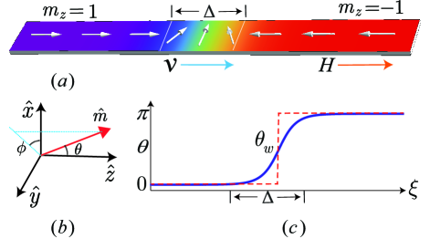
Figure 1: (Color online) (a) Illustration of transverse head-to-head DW of width $\Delta$ in a nanowire, with easy axis along $\hat{z}$ and hard axis along $\hat{x}$. In the absence of external magnetic field (upper), a static DW exists between two domains with $m_{z}=\pm 1$. Under a field parallel to the easy axis, the Walker propagating DW moves towards the energy minimum state ($m_{z}=-1$) at a speed $v$ while the DW profile is preserved. (b) Illustration of coordinate system. (c) Solid line:DW profile $\theta_{w}$ vs. $\xi$ that varies noticeably around the DW center. Dashed line: local perturbation to $\theta_{w}$.

However, unlike stability analysis of solutions of linear and nonlinear ordinary differential equations which can be easily done by using the linearization techniques and Lyapunov-exponent concept [18, 19], it is hard in general for nonlinear partial differential equations like the LLG equation. Although numerical approaches can provide clues and hints, an analytical approach is lack for Walker solution until recently the progress of traveling wave analysis suggests a feasible way. In this paper, we shall present in detail the method and results of our stability analysis of the Walker exact propagating DW solution of a 1+1 dimensional LLG equation [20]. It is shown that a propagating DW is always dressed with spin waves so that the Walker solution is not stable against spin-wave emission. In the low field region, only stern spin waves are emitted while both stern and bow waves emerge under high field. When the transverse magnetic anisotropy is larger than a critical value and the external field is sufficiently high, the solution is convective or absolute unstable, corresponding to severe distortion of the propagating DW profile. This shall lead to noticeable deviation of DW speed from the Walker formula besides that the DW is dressed with spin waves. The paper is organized as follows. The model and theoretical formulation are explained in the next section. Section III is the results and discussions, and the conclusion is in Section IV.

II II. MODEL AND THEORETIC FORMULATION

To study the stability of Walker exact propagating DW solution under an external field, we consider the dimensionless LLG equation [7],

$$\frac{\partial\vec{m}}{\partial t}=-\vec{m}\times{\vec{h}_{eff}}+\alpha\vec{m}\times\frac{{\partial\vec{m}}}{{\partial t}}.$$ (1)

This LLG equation describes the dynamics of the magnetization $\vec{M}$ of a magnetic nanowire schematically shown in Fig. 1. With the easy axis along the wire ($\hat{z}$ direction) and the width and thickness being smaller than the exchange interaction length, exchange interaction dominates the stray field energy caused by magnetic charges on the edges; the DW structure tends to be homogeneous in the transverse direction [21], i.e., behaves effectively 1D. We are interested in the behavior of a head-to-head DW under an external field shown in Fig. 1. In Eq. (1), $\vec{m}$ is the unit direction of the local magnetization $\vec{M}=\vec{m}M_{s}$ with saturation magnetization $M_{s}$ and $\alpha$ is the phenomenological Gilbert damping constant. The effective field (in units of $M_{s}$) is $\vec{h}_{eff}=K_{\parallel}m_{z}\hat{z}-K_{\perp}m_{x}\hat{x}+A\partial^{2}\vec{m}/\partial z^{2}+H\hat{z}$ where $K_{\parallel}$, $K_{\perp}$, and $A$ are respectively the easy axis anisotropy coefficient, the hard axis anisotropy coefficient, and the exchange coefficient. $H$ is the external magnetic field parallel to $\hat{z}$. The time unit is $(\gamma M_{s})^{-1}$, where $\gamma$ is the gyromagnetic ratio. Using polar angle $\theta$ and azimuthal angle $\varphi$ for $\vec{m}$ as shown in Fig. 1, this LLG equation has a well known Walker propagating DW solution [1],

$$\begin{split}\sin 2{{\varphi_{w}(z,t)}}=\frac{H}{H_{c}},\quad\ln\tan\frac{1}{2}{\theta_{w}(z,t)}=\frac{z-vt}{\Delta}.\end{split}$$ (2)

Here $H_{c}=\alpha K_{\perp}/2$ is the Walker breakdown field and $\Delta={(K_{\parallel}/A+{\cos^{2}}{\varphi_{w}}K_{\perp}/A)^{-1/2}}$ is the DW width which will be used as the length unit ($\Delta=1$) in the analysis below. $v=\Delta H/\alpha$ is the Walker rigid-body DW speed that is linear in the external field and the DW width, and inversely proportional to the Gilbert damping constant. Solution (2) is exact for $H<H_{c}$.

In the following analysis, the meaning of stability/instability of the DW is confined to Lyapunov definition, i.e., the DW is stable if any other solution of Eq. (1) starting close enough to the Walker solution will remain close to it forever; otherwise it is unstable. We will prove the instability of solution (2) against spin-wave emission by performing a spectrum analysis according to a recent developed theory for a general travelling front, such as a propagating head-to-head DW shown in Fig. 1. To prove the instability of solution (2), we follow a recently developed theory (Sandstede and Scheel [23] and Fiedler and Scheel [24]) for stability of a general traveling front, that is, a solution connecting two homogeneous states, such as a propagating head-to-head DW shown in Fig. 1. A modus operandi is to perturb Eq. (1) by a small deviation $\vec{\delta}$ from the solution (2) via which an evolution equation governing this deviation can be derived. Note that if we directly perturb Eq. (1) by $m_{x}^{w}+\delta_{x}$, $m_{y}^{w}+\delta_{y}$ and $m_{z}^{w}+\delta_{z}$, with $|\delta_{x,y,z}|\ll 1$ ($m_{x}^{w}$, $m_{y}^{w}$ and $m_{z}^{w}$ are components of Eq. (2) in the Cartesian coordinates), the three components of $\vec{\delta}$ were not independent due to the preservation of $\text{ }\!\!|\!\!\text{ }\vec{M}\text{ }\!\!|\!\!\text{ }$. A convenient way to circumvent this problem is, instead of analyzing in the Cartesian space, to work with the polar-coordinate form of Eq. (1) in which the two variables $\theta$ and $\phi$ satisfy [1]:

$$\begin{array}[]{l}\dot{\theta}-\alpha\sin\theta\dot{\varphi}=-2{K_{\bot}}\sin\theta\sin\varphi\cos\varphi+4A\theta^{\prime}\varphi^{\prime}\\ \;\;\;\;\;\;\;\;\;\;\;\;\;\;\;\;\;\;{\rm{+}}2A\sin\theta\varphi^{\prime\prime},\\ \sin\theta\dot{\varphi}+\alpha\dot{\theta}=-2{K_{\bot}}\sin\theta\cos\theta{\cos^{2}}\varphi+2{K_{//}}\sin\theta\cos\theta\\ \;\;\;\;\;\;\;\;\;\;\;\;\;\;\;\;\;\;+H\sin\theta{\rm{+}}2A\sin\theta\cos\theta{{\varphi^{\prime}}^{2}}-2A\theta^{\prime\prime},\end{array}$$ (3)

where single and double prime denote the first and the second derivatives with respect to $z$. By assuming $\theta_{w}+\theta$ and $\varphi_{w}+\varphi$ the solution of Eq. (3) with $|\theta|$, $|\varphi|\ll 1$, and by keeping only the terms of the first order in $\theta$ and $\varphi$, the linearized equations of $\theta$ and $\varphi$ in the moving DW frame of velocity $v$ (with the coordinate transformation $z\to\xi$ and $t\to t$, where $\xi=z-vt$) are, in a two-component form of $\Lambda\equiv{{(\theta,\ \varphi)}^{T}}$ (superscript $T$ means transpose),

$$\frac{{d\Lambda}}{{dt}}={L_{0}}\Lambda+{L_{1}}\frac{{\partial\Lambda}}{{\partial\xi}}+{L_{2}}\frac{{{\partial^{2}}\Lambda}}{{\partial{\xi^{2}}}},$$ (4)

where $L_{0}$, $L_{1}$, and $L_{2}$ are $2\times 2$ matrices that depend on $\xi$ through ${{\theta}_{w}}$. $L_{0}$ has the following matrix elements: $L_{0,11}=\{\alpha K_{\parallel}\cos[2G(\xi)]+K_{\bot}(\sqrt{1-{\rho^{2}}}-1)\cos[2G(\xi)]/2+(H\alpha-K_{\bot}\rho/2)\tanh\xi\}/(1+\alpha^{2})$, $L_{0,21}=\{K_{\parallel}\cosh\xi\cos[2G(\xi)]+K_{\bot}(\sqrt{1-\rho^{2}}-1)\cosh\xi\cos[2G(\xi)]/2+(H+K_{\bot}\alpha\rho/2)\sinh\xi\}/(1+\alpha^{2})$, $L_{0,12}=$sesh$\xi K_{\bot}(-\sqrt{1-\rho^{2}}+\alpha\rho\tanh\xi)/(1+\alpha^{2})$, $L_{0,22}=K_{\bot}(\alpha\sqrt{1-\rho^{2}}+\rho\tanh\xi)/(1+\alpha^{2})$. Here $G(\xi)$ is the Gudermannian function and $\rho=H/H_{c}$. $L_{1}$, $L_{2}$ can be expressed explicitly in terms of $\xi$ as:

$$\begin{array}[]{l}L_{1}{\rm{=}}\left({\begin{array}[]{*{20}{c}}v&{-\frac{{2A}}{{(1+{\alpha^{2}})\cosh\xi}}}\\ 0&{v+\frac{{2A\alpha}}{{(1+{\alpha^{2}})}}}\end{array}}\right),\\ L_{2}{\rm{=}}\frac{1}{{(1+{\alpha^{2}})}}\left({\begin{array}[]{*{20}{c}}{A\alpha}&{-\frac{A}{{\cosh\xi}}}\\ {A\cosh\xi}&{A\alpha}\end{array}}\right).\end{array}$$

Eq. (4) is a linearized equation, and its general solutions are linear combinations of basic solutions of the form,

$$\Lambda(\xi,t)={\Lambda_{1}}(\xi){e^{\lambda t}},$$ (5)

where $\lambda$ is a proper complex number that supports nontrivial solutions (not constant zero) for equation

$$(L-\lambda){\Lambda_{1}}\left(\xi\right)=0,$$ (6)

where $L=L_{0}+L_{1}\partial/\partial\xi+L_{2}\partial^{2}/\partial\xi^{2}$. Then all such $\lambda$ define the spectrum of $L$. It is straightforward to verify that, due to translational invariance of solution (2), $\lambda=0$ always belongs to the spectrum, with the corresponding eigenfunction ${\Lambda_{1}}={({{\partial{\theta_{w}}}}/{{\partial\xi}},{{\partial{\varphi_{w}}}}/{{\partial\xi}})^{T}}.$ If none of $\lambda$ in the spectrum has positive real part, the spectrum is said to be stable; otherwise it is unstable. For a stable spectrum, any moderate deviations from the Walker solution must either decay exponentially with time [$\operatorname{Re}(\lambda)<0$] or undergo periodic motion by retaining its amplitude [$\operatorname{Re}(\lambda)$$=0$]. When the spectrum encroaches the left half plane, exponentially growing modes ($\operatorname{Re}(\lambda)$$>0$) exist. We shall use so-called essential and absolute spectra of $L(\xi)$ to decide the stabilities/instabilities of domains and DW profile.

III III. RESULTS AND DISCUSSIONS

III.1 A. ESSENTIAL INSTABILITY

In order to compute the spectrum of $L(\xi)$, it is convenient to rewrite Eq. (6) in the first order differential form by using $\Omega\equiv(\theta,\;\varphi,\;\partial\theta/\partial\xi,\;\partial\varphi/\partial\xi)^{T}$,

$$\frac{d}{{d\xi}}\Omega=\Gamma(\lambda,\xi)\Omega,$$ (7)

where

$$\Gamma(\lambda)=\left({\begin{array}[]{*{20}{c}}0&I\\ L_{2}^{-1}(\lambda-L_{0})&-L_{2}^{-1}L_{1}\end{array}}\right).$$ (8)

$I$ is the $2\times 2$ identity matrix. All $\lambda$ that supports nontrivial solutions to Eq. (7) form its spectrum. Eq. (6) and Eq. (7) have the same spectrum because they are equivalent. We shall focus hereafter on the spectrum of Eq. (7). To do so, we need to obtain the conditions under which Eq. (7) has nontrivial solutions. Let us first divide $\xi$ axis into four regions: $\xi\leq-l$, $-l\leq\xi\leq 0$, $0\leq\xi\leq l$ and $\xi\geq l$ with $l\gg\Delta$. Notice that $\Gamma$ depends on $\xi$ only through $\theta_{w}$ that varies with $\xi$ only within the DW, Eq. (7) is essentially,

$$\frac{d}{d\xi}\Omega=\Gamma^{-}(\lambda)\Omega.$$ (9)

in region $-\infty<\xi\leq-l$ and

$$\frac{d}{d\xi}\Omega=\Gamma^{+}(\lambda)\Omega.$$ (10)

in region $l\leq\xi<\infty$. The two asymptotic matrices $\Gamma^{\pm}$ are,

$$\Gamma^{\pm}\left(\lambda\right)=\lim_{\xi\to\pm\infty}\Gamma(\lambda,\xi).$$ (11)

$\Gamma^{\pm}$ can be directly obtained from Eq. (8) by replacing $\theta_{w}(\xi)$ with $\pi$ for $+$ and with $0$ for $-$. In region $-\infty<\xi\leq-l$ ($l\leq\xi<\infty$) and for each given $\lambda$, $\Gamma^{\pm}(\lambda)$ has 4 eigenvalue and eigenvector pairs, $(\kappa^{\pm}_{i},\mu^{\pm}_{i})$ $i=1,\ldots,4$, and Eq. (9) ((10)) has solution of form $\mu_{i}^{-}e^{\kappa_{i}^{-}\xi}$ ($\mu_{i}^{+}e^{\kappa_{i}^{+}\xi}$). $\lambda$ can then be denoted by $(n^{\pm}_{+},n^{\pm}_{-})$ for $n^{\pm}_{+}$ ($n^{\pm}_{-}$) being the number of $\kappa^{\pm}(\lambda)$ with positive (negative) real parts. Obviously, we have $n^{+}_{+}+n^{+}_{-}=n^{-}_{+}+n^{-}_{-}=4$ except on the so-called Fredholm borders explained below in detail. $\kappa^{\pm}$ can then be ordered descending by their real parts as ${\mathop{\rm Re}\nolimits}(\kappa_{1}^{\pm})\geq...\geq{\mathop{\rm Re}\nolimits}(\kappa_{n_{+}^{\pm}}^{\pm})>0>{\mathop{\rm Re}\nolimits}(\kappa_{n_{+}^{\pm}+1}^{\pm})\geq...\geq{\mathop{\rm Re}\nolimits}(\kappa_{4}^{\pm})$. Each solution $\mu_{i}^{-}e^{\kappa_{i}^{-}\xi}$ ($\mu_{i}^{+}e^{\kappa_{i}^{+}\xi}$) in region $-\infty<\xi\leq-l$ ($l\leq\xi<\infty$) can be continued into region $-l\leq\xi\leq 0$ ($0\leq\xi\leq l$) as $\Omega_{i}^{(}\xi)$ ($\Omega_{i}^{+}(\xi)$). Suppose we are interested in a nontrivial bounded solution $\Omega$ of Eq. (7), i.e., $\Omega(\pm\infty)=0$, then $\Omega$ must be the linear superposition of those $\Omega_{i}^{-}(\xi)$ [$\Omega_{i}^{+}(\xi)$] in $-l\leq\xi\leq 0$ ($0\leq\xi\leq l$) whose corresponding eigenvalues $\kappa_{i}^{-}$ ($\kappa_{i}^{+}$) have positive (negative) real parts. Note that the number of $\kappa_{i}^{-}$ ($\kappa_{i}^{+}$) with Re$(\kappa_{i}^{-})>0$ (Re$(\kappa_{i}^{+})<0$) is $n^{-}_{+}$ ($n^{+}_{-}$), whether or not such $\Omega$ exists is equivalent to whether or not we can find nontrivial solution $(a_{i},b_{j})$ satisfying

$$\sum\nolimits_{i=n_{+}^{+}+1}^{4}a_{i}\Omega_{i}^{+}(0)=\sum\nolimits_{j=1}^{n_{+}^{-}}b_{j}\Omega_{i}^{-}(0).$$ (12)

This is the condition of the continuation of $\Omega$ at $\xi=0$. The spectrum of Eq. (7) is the set of all $\lambda$ such that Eq. (12) has at least one nonzero solution of $(a_{i},b_{j})$ for $i=n_{+}^{-}+1\ldots 4$ and $j=1\ldots n_{+}^{-}$. Obviously, there are $n_{-}^{+}+n_{+}^{-}$ variables and 4 equations. The existence of such a solution is then $n_{-}^{+}+n_{+}^{-}>4$. The explict solutions of $(a_{i},b_{j})$ require the knowledge of $\Omega_{i}^{\pm}(0)$ that is normally not known analytically because of the complicate $\xi$-dependence of $\Gamma(\lambda,\xi)$. Numerical method such as the shooting algorithm used in the Schrodinger equation may be use here by numerically integrating Eq. (7) starting from $\xi=\pm l$ (where all linear independent solutions of Eqs. (9) and (10) are known) and ending at $\xi=0$. Correct set of $(a_{i},b_{j})$ shall make the shooting of $\Omega$ from $\xi=\pm l$ end with the same value at $\xi=0$. The shooting algorithm, proved to be efficient for the Schrodinger equation whose spectrum is on the real line, may become excessively arduous for the LLG Eq. where the spectrum extends to the whole complex plane. As we shall see, this formidable task can be partly dodged as far as only the essential instability is considered which is pertinent to spin wave emissions.

Similar to the energy spectrum of a quantum system, the spectrum $\lambda$ of Eq. (7) can be discrete and continuum. The continuum $\lambda$ is also called the essential spectrum. The essential spectrum is not sensitive to the so called relatively compact perturbations to Eq. (7). Here a relatively compact perturbation can be understood, in some senses, as a local perturbation to a Schrodinger equation

$$[-\frac{{{d^{2}}}}{{d{x^{2}}}}+V(x)]\psi=E\psi.$$

This continuous spectrum will not be changed by a $V(x)$ of finite potential range, such as a potential well or barrier, although wave functions are altered and point spectrum may be introduced. According to [26, 25, 24, 23], a similar local perturbation to Eq. (7) (or in general to any linearized equation of a system around a front solution) preserve the essential spectrum so that we can replace $\theta_{w}$ (Fig. 1 (c)) by $\pi H(\xi)$, where $H(\xi)$ is the Heaviside step function. The new equation with the same essential spectrum as that of Eq. (7) is

$$\frac{d}{{d\xi}}\Omega=\Gamma^{\infty}\Omega,$$ (13)

where

$${\Gamma^{\infty}}\equiv\left\{\begin{array}[]{l}{\Gamma^{+}(\lambda)},\;\;\;\;\;\;\xi\geq 0\\ {\Gamma^{-}(\lambda)},\;\;\;\;\;\;\xi<0\end{array}\right.$$ (14)

$\Gamma^{\pm}(\lambda)$ have already been defined in Eq. (11). Since $\Gamma^{\infty}$ is constant in each region of $(-\infty,0)$ and $(0,\infty)$, the corresponding $\Omega_{i}^{\pm}$ in Eq. (12) are just eigenvectors $\mu_{i}^{\pm}$ of $\Gamma^{\pm}$. Therefore Eq. (12) becomes

$$\sum\nolimits_{i=n_{+}^{+}+1}^{4}a_{i}\mu_{i}^{+}=\sum\nolimits_{j=1}^{n_{+}^{-}}b_{j}\mu_{j}^{-}.$$ (15)

Eq. (15) have nonzero solution if the number of variables $a_{i}$ and $b_{j}$, $n_{-}^{+}-n_{+}^{-}$, is greater than 4. Thus, Eq. (13) has nontrivial solution bounded at $\xi=\pm\infty$ for all $\lambda$ whose $n_{-}^{+}+n_{+}^{-}>4$. If one allow other types of solutions at $\xi=\pm\infty$, then the general condition is $n_{-}^{+}+n_{+}^{-}\neq 4$. Indeed according to the theory of Refs. [23, 22, 25, 24, 26], the essential spectrum of $L$ (also of Eq. (7) and/or Eq. (13)) is the union of all closed sets of $\lambda$ (boundaries included) whose indices $n_{-}^{+}$ and $n_{+}^{-}$ satisfy $n^{+}_{-}+n^{-}_{+}\neq 4$. The boundaries of each region, known as the Fredholm borders, must be those lines crossing which either $n^{+}_{-}$ or $n^{-}_{+}$ changes its value by 1. Then along each Fredholm border, either $\Gamma^{+}$ or $\Gamma^{-}$ must possess pure imaginary eigenvalue (not a hyperbolic matrix); thus these lines can be determined by $\det[\Gamma^{\pm}(\lambda)+ik]=0$ with $k\in(-\infty,\infty)$ [23, 22, 24]. Each of the two equations has two branches of allowed $\lambda$ denoted as $\lambda_{1,2}^{\pm}(k)$. Note that Eqs. (9) and (10) admit pure plane wave solution $\Omega_{0}e^{ik\xi}$ when $\lambda$ is on $\lambda_{1,2}^{+}(k)$ ($\lambda_{1,2}^{-}(k)$). Therefore an encroachment of these borders to the right half plane implies spin wave emission. We refer to the type of instability characterized by the presence of essential spectrum on the right half plane as the essential instability.

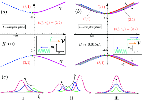
Figure 2: (Color online) Left are the essential spectrum (shadowed regions) for $H=0$ (a) and $H\approx 0.015H_{c}$ (b). The Fredholm borders are $\lambda_{1,2}^{\pm}(k)$. Solid border lines correspond to spin waves with negative group velocities while the dashed border lines are for the spin waves with positive group velocities. Propagating DW wall emit stern waves in low fields [right of (a)], and stern and bow waves in higher field ($0.015H_{c}<H<H_{c}$) [right of (b)]. The green dots are zero group velocity modes. $K_{\perp}=0.4$ is used. (c) Illustration of transient instability (i) in which the unstable mode travels to only one direction; convective instability (ii) in which the unstable mode travels to both directions; and the absolute instability (iii) in which the unstable mode does not travel (stationary in the moving frame).

In order to understand numerical results in Ref. [13], parameters of yttrium iron garnet (YIG) [17] are assumed in our analysis with $A=3.84\times 10^{-12}J/m$, $K_{\parallel}=2\times 10^{3}J/m^{3}$, $\gamma=35.1kHz/(A/m)$, and $M_{s}=1.94\times 10^{5}A/m$. $\alpha=0.001$ is used and $K_{\perp}$ is a varying parameter. Fig. 2 plots the essential spectrum for $K_{\perp}=0.4$ (in units of $\mu_{0}M_{s}^{2}$ that is about 10 times larger than $K_{\parallel}$). The qualitative results are very similar to the early results [20]: In the absence of an external field, the two branches of the spectrum of $\Gamma^{\pm}$ are the same, $\lambda_{1,2}^{+}(k)=\lambda_{1,2}^{-}(k)$, shown in Fig. 2(a). Since the spectrum encroaches the right half plane, unstable plane waves shall exist and spin wave emission are expected. Similar conclusion was also obtained in early study [27], but for $H>H_{c}$. Solid lines are for negative group velocity [determined by Im$({\partial\lambda}/{\partial k})$], thus these are stern modes. The dashed lines indicate positive group velocity, corresponding to bow modes. The green dots are zero group velocity points. According to Fig. 2(a), all unstable modes have negative group velocities so that DW can only emit stern waves in the low fields. As the external field increases, $\lambda_{1,2}^{+}(k)$ and $\lambda_{1,2}^{-}(k)$ will separate, and the area of essential spectrum in $\lambda$-plane becomes bigger and bigger (shadowed regimes in Fig. 2(b). The green dots also moves toward Im$(\lambda)$-axis and cross it at $H\approx 0.015H_{c}$ [Fig. 2(b)]. Upon further increase of $H$, the unstable modes have both positive and negative group velocities although the most of them have the negative ones. One shall have propagating DW to emit both stern and bow waves. The stern waves should be stronger than the bow waves as schematically shown in the right figure of Fig. 2(b). This is exactly what were observed in numerical simulations for stern wave emission in low field [12] and stern-and-bow wave emission in high field [13]. In a realistic wire with damping, emitted spin waves will be dissipated after a short distance, and are hard to be observed in experiments.

III.2 B. TRANSIENT/CONVECTIVE/ABSOLUTE INSTABILITY

The essential spectrum decides the instability of domains. DW propagation will generate spin waves in domains when the essential spectrum encroaches the right half of the $\lambda$ plane. The fact that the essential spectrum is not affected by the variation of DW profile means that the essential spectrum cannot determine the instability of DW profile that is important for many quantities such as the DW velocity. Interestingly, DW instability is determined by the so-called absolute spectrum explained below. It can be classified into three categories. Absolute instability [AI, Fig. 2(c)iii] occurs when at each fixed point on the $\xi$-axis, the disturbance grows exponentially with time. It is associated with the emergence of nontraveling unstable modes in the absolute frame (the moving frame that we adopted); thus coins its name. This point-wise growth feature of AI is in sharp contrast with the other two types of instability, which albeit grows in the total norm, decays locally at each fixed point on the $\xi$-axis. They happens when all unstable modes are transported to infinities at fast enough velocities. It is called a transient instability (TI, Fig. 2(c)i) if the disturbance generated locally in the DW region transports to infinity in one direction (either towards $\infty$ or $-\infty$), while it is called convective (CI, Fig. 2(c)ii) if it can transport in both directions. Intuitively, transient instability shall have the least influence on the DW property since once generated, it will leave the DW region quickly and will not interact with the DW hereafter. Convective instability is stronger than the transient one since although transported outside the DW region, it could influence the DW through second order effect in which new bidirectional unstable modes excited by the convecting wave packets can collide and interact with the DW again. Absolute instability is the most severe one in the sense that once a nontraveling disturbance is generated, it can stay within and keep interacting with the DW, leading to dramatic modification on the DW profile. For this reason, physical quantities depending on DW profile, such as the DW velocity, are expected to be strongly affected.

The three types of transportation behavior, either unidirectional, bidirectional or non-travelling, are determined by the so-called absolute spectrum and the branching points [23, 22, 25, 24, 26, 30, 28, 29]. To introduce the absolute spectrum and the branching points, we recall that, for each $\lambda$ in the complex plane, there are four $\kappa_{i}^{\pm}$ ($i=1,2,3,4$) for $\Gamma^{\pm}$, ordered by their real parts as $\hbox{Re}(\kappa_{1}^{\pm})\geq\hbox{Re}(\kappa_{2}^{\pm}\geq\hbox{Re}(\kappa_{3}^{\pm})\geq\hbox{Re}(\kappa_{4}^{\pm})$. Then $\lambda$ is said to belong to the absolute spectrum ($\lambda_{abs}$) if and only if $\hbox{Re}[\kappa_{2}^{+}(\lambda)]=\hbox{Re}[\kappa_{3}^{+}(\lambda)]$ or $\hbox{Re}[\kappa_{2}^{-}(\lambda)]=\hbox{Re}[\kappa_{3}^{-}(\lambda)]$. The branching points are special points in the absolute spectrum, denoted as $\lambda_{sd}$, satisfying $\kappa_{2}^{\pm}(\lambda_{sd})=\kappa_{3}^{\pm}(\lambda_{sd})$. To have a better feeling about the absolute spectrum and differences in unidirectional/bidirectional transportation and nontraveling modes of a wave $\Lambda(z,t)$, we introduce the concept of pointwise decay and growth. A wave $\Lambda(z,t)$ is said to be pointwise decay iff $\lim_{t\to\infty}\Lambda(z_{0})=0$ for any fixed $z_{0}$. The opposite ($\infty$ instead of 0) is said to be pointwise growth. Let us first consider a wavelet that may exemplify a transient disturbance transporting to the right along the z axis:

$$\Lambda=e^{\lambda t}\hbox{sech}(z-vt).$$ (16)

This is an unstable mode if $\hbox{Re}(\lambda)>0$. At each fixed point $z_{0}$, $\lim_{t\to\infty}\Lambda(z_{0})=0$ ($\infty$) if $v>\hbox{Re}(\lambda)$ ($v<\hbox{Re}(\lambda)$). In another word, an unstable disturbance moving fast enough can lead to pointwise decay (vanish in a long time at each fixed point) although its norm $\|\Lambda\|=\int_{-\infty}^{\infty}\left|\Lambda\right|^{2}dz=\pi e^{\lambda t}$ increases exponentially with time. Interestedly, (16) can be brought to be stable when $v>\hbox{Re}(\lambda)$ if an exponential weight $e^{\eta z}$ is used

$$\|\Lambda\|_{\eta}=\int_{-\infty}^{\infty}\left|e^{\eta z}\Lambda\right|^{2}dz=e^{\lambda^{\prime}t}C_{0},$$ (17)

where

$$\lambda^{\prime}=2(\lambda+\eta v)$$

and

$$C_{0}=\int_{-\infty}^{\infty}e^{2\eta z^{\prime}}{\mathop{\rm sech}\nolimits}^{2}(z^{\prime})dz^{\prime}.$$

Note that the integral $C_{0}$ is finite whenever $|\eta|<1$. Therefore any $-1<\eta<-[\hbox{Re}(\lambda)/v]$ makes $\hbox{Re}(\lambda^{\prime})<0$ such that the new norm (17) decay exponentially with time. However, if $v<\hbox{Re}(\lambda)$, either (17) diverges with time or $C_{0}$ is infinity for any $\eta$. In another word, the mode becomes stable under a proper exponential weight $\|.\|_{\eta}$ for $v>\hbox{Re}(\lambda)$, and a transient disturbance traveling towards $-\infty$ fast enough can be stabilized by a positive $\eta$ since then the multiplier $e^{\eta z}$ balance the growing modes at $-\infty$.

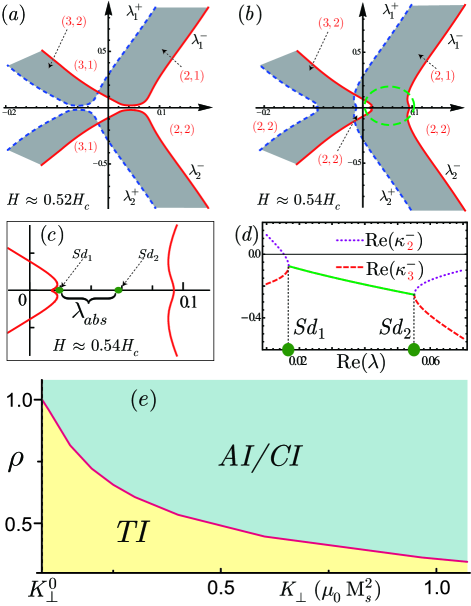
Figure 3: (Color online) Essential spectra and $(n^{+}_{-},n^{-}_{+})$ in regions divided by $\lambda^{\pm}_{1,2}$ for $K_{\perp}=0.4$, $\rho=0.52$ (a) and $0.54$ (b). No absolute spectrum presents before $\lambda^{\pm}_{1,2}$ tangents at the real axis while in (b), unstable absolute spectrum presents in the region enclosed by the solid circle. (c) Enlarged description of the region enclosed by the solid circle in (b). The absolute spectrum is between the two branching points $Sd_{1}$ and $Sd_{2}$ (green dots). (d) Plot of $\hbox{Re}(\kappa^{-}_{2})$ and $\hbox{Re}(\kappa^{-}_{3})$ vs. $\lambda$ between $Sd_{1}$ and $Sd_{2}$. At $Sd_{1,2}$, $\kappa^{-}_{2}=\kappa^{-}_{3}$. (e) Phase diagram of transient (TI) and absolute/convective (AI/CI) instabilities. The boundary is the bifurcation line between TI/CI-and-CI instabilities in $K_{\perp}$ and $\rho=H/H_{c}$ plane. The bifurcation line is only plotted for $K_{\perp}\geq K_{\perp}^{0}$ here $K_{\perp}^{0}\approx 0.085$ at which $H_{2}=H_{c}$ ($\rho=1$). Noted that our analysis is valid for fields below the Walker breakdown value.

In general, the exponentially weighted norm denoted by $\left\|\cdot\right\|_{\eta}$ for a real number $\eta$ is defined as

$$\left\|\Lambda\right\|_{\eta}\equiv\int_{-\infty}^{\infty}\left|e^{\eta\xi}\Lambda\right|^{2}d\xi.$$ (18)

The transient and convective instabilities behave very differently under the norm. For a given $\lambda$, its eigenmode is transient unstable if it has an exponentially growing factor that travels towards $-\infty$ (or $\infty$). Under an exponentially weighted norm with a proper choice of $\eta>0$ ($\eta<0$) for mode traveling to $-\infty$ ($\infty$), the growth at $-\infty$ ($\infty$) can be absorbed by the multiply $e^{\eta\xi}$. Therefore the essential spectrum calculated under the exponential norm With $\eta>0$ ($\eta<0$) can be transferred to the left half of the $\lambda$ plane for the unidirectional modes traveling towards $-\infty$ ($\infty$). Mathematically, this corresponds to a proper choice of the origin of the $\lambda$ plane in some sense. Thus, with the proper definition of the norm by choosing a large enough $|\eta(\lambda)|$, all unstable unidirectional eigenmodes of eigenvalues $\lambda$ (essential spectrum in the right half of the $\lambda$ plane) are removable because all such $\lambda$ can be transferred to the left half of the $\lambda$ plane. This treatment fail to the modes traveling to both directions of $\xi=\pm\infty$ (bidirectional eigenmodes). They are not removable since an exponential weight can only suppress the growth in one direction and blow up in the other direction. The ability/inability of using an exponential weight (18) to stabilize/destabilize transient/convective modes leads to the following properties: TI occurs if all unstable essential spectrum can be move to the left half $\lambda$ plane under a proper exponentially weighted norm while it is CI or AI if part of the unstable essential spectrum cannot be stabilized by the norm. A naturally raised question then is which part of the essential spectrum cannot be removed by this weight.

The answer is quite simple: The absolute spectrum cannot be moved around in the $\lambda$ plane by introducing an exponential weight. It must locate to the left of the rightmost Fredholm border. If it encroaches the right half of the $\lambda$ plane, then the essential spectrum cannot be stabilize no matter how one chose the exponential weight $\eta$. To see why this is so, it is noticed that we need to introduce a weight $\eta^{-}(\lambda)$ [$\eta^{+}(\lambda)$] in order to move the Fredholm border determined by Eq. (9) [(10)]. Thus, by using the exponential weight of $\eta^{\pm}$, it is equivalent to shift the eigenvalues of $\Gamma^{\pm}$ [23, 22, 25, 24, 26, 30, 28, 29] by

$$\kappa_{i}^{\pm}\to\tilde{\kappa}_{i}^{\pm}\equiv\kappa_{i}^{\pm}-{\eta^{\pm}},$$ (19)

and accordingly the indices of the $\lambda$ are transformed as

$$(n_{-}^{+},n_{+}^{-})\to(\tilde{n}_{-}^{+},\tilde{n}_{+}^{-}),$$ (20)

Now suppose $\lambda$ with $\hbox{Re}(\lambda)>0$ belongs to the Essential spectrum but not on the Fredholm border, which means $n_{-}^{+}+n_{+}^{-}\neq 4$. For the LLG equation and independent of the norm we use, $\lambda$ in the right hand side of the rightmost Fredholm border has the indices of $n_{-}^{+}=n_{+}^{-}=2$, then all possible combinations of $(n_{-}^{+},n_{+}^{-})$ in the regions right after passing through the rightmost Fredholm border can only be one of the four cases: $(1,2)$, $(2,1)$, $(2,3)$, $(3,2)$. Consider for instance $(n_{-}^{+},n_{+}^{-})=(1,2)$, then obviously $\hbox{Re}(\kappa^{-}_{2})>0>\hbox{Re}(\kappa^{-}_{3})$ and $\hbox{Re}(\kappa^{+}_{2}),\ \hbox{Re}(\kappa^{+}_{3})>0$. If we also have $\hbox{Re}(\kappa^{+}_{2})\neq\hbox{Re}(\kappa^{+}_{3})$, i.e. $\lambda\notin\lambda_{abs}$, we could always find the aforementioned proper weight as, for instance:

$${\eta^{\pm}}=\left\{\begin{array}[]{l}{\eta^{\rm{+}}}{\rm{=}}\frac{{{\mathop{\rm Re}\nolimits}(\kappa_{2}^{+}){\rm{+}}{\mathop{\rm Re}\nolimits}(\kappa_{3}^{+})}}{2},\\ {\eta^{-}}=0,\end{array}\right.$$ (21)

which means that, for essential spectrum calculated under this norm, $\lambda$ is well to the right of the essential spectrum. We can thus remove all unstable $\lambda$ (i.e., $\hbox{Re}(\lambda)>0$) in this way if there is no $\lambda_{abs}$ on the right half of the $\lambda$ plane. However, if $\lambda$ belongs to $\lambda_{abs}$ such that $\hbox{Re}(\kappa^{+}_{2})=\hbox{Re}(\kappa^{+}_{3})$, it is easy to verify that no such pair of $\eta^{\pm}$ exist. This absolute spectrum is exactly the set of $\lambda$ which could not be stabilized by the aforementioned proper weights $\eta^{\pm}$. Therefore we conclude that the absence of $\lambda_{abs}$ in the right half of the $\lambda$ plane indicate Transient instability in which all eigenmodes are unidirectional while the presence of the absolute spectrum means emergence of bidirectional eigenmodes.

Finally, the presence of unstable non-traveling modes is associated with the branching points’s presence on the right half plane. It is straightforward to verify that the eigenmodes associated with these branching points have zero group velocity, as follows. Denote the secular polynomial of $\Gamma^{\pm}(\lambda)$ as: $F(\lambda,\kappa)\equiv\det[\Gamma^{\pm}(\lambda)-\kappa I].$ Then for $\lambda_{sd}$ satisfying $\kappa_{2}^{\pm}({\lambda_{sd}})=\kappa_{3}^{\pm}({\lambda_{sd}})$, it must hold that:

$$F({\lambda_{sd}},\kappa)={(\kappa-\bar{\kappa})^{2}}(\kappa-{\kappa_{1}})(\kappa-{\kappa_{4}}),$$ (22)

where $\bar{\kappa}\equiv{\kappa_{2}}{\rm{=}}{\kappa_{3}}$. Then the group velocity $v$ of modes associated with $\lambda_{sd}$ is

$$v={\mathop{\rm Im}\nolimits}\left({\frac{\partial\lambda}{\partial\kappa}}\right)\left|{}_{\kappa{\rm{=}}\bar{\kappa},\\ \lambda=\lambda_{sd}}\right.={\mathop{\rm Im}\nolimits}\left(-\frac{\partial_{k}F}{\partial_{\lambda}F}\right)\left|{}_{\kappa{\rm{=}}\bar{\kappa},\lambda=\lambda_{sd}}\right.=0.$$ (23)

Thus, branching points $\lambda_{sd}$ are non-travelling eigenmode [30, 33]. For $K_{\perp}=0.4$, the absolute spectrum in the right half of the $\lambda$ plane is generated by $\Gamma^{-}$. Fig. 3(a) shows two branches $\lambda_{1,2}^{-}$. They are well separated by the real axis for $\rho=0.52$ and no absolute spectrum could be found in the right half plane. As the field increases, the two branches get closer with each other and at an onset field $H_{2}$, depending on $K_{\perp}$, two branches tangent at the real axis and then separate again in horizontal direction as shown in Fig. 3(b) for $\rho=0.54$. At this moment, unstable absolute spectrum begins to emerge on the real axis (enclosed by the dashed circle). Fig. 3(c) is the enlarged vision showing the absolute spectrum (the segment between two branching points $Sd_{1,2}$ (green solid dots)). The dependence of $\hbox{Re}(\kappa_{2}^{-})$ or $\hbox{Re}(\kappa_{3}^{-})$ on $\hbox{Re}(\lambda)$ between these two points is shown in Fig. 3(d).

According to Refs. [30, 28, 29], wavepackets would be emitted if the essential spectrum encroaches the right half $\lambda$-plane. There are three types of instability [23, 22, 24, 25, 30, 28, 29]. The instability is called transient (TI) if the essential spectrum encroaches the right half plane and absolute spectrum are either in the left half plane or does not exist. The propagating DW emits stern waves shown in Fig. 2(c)i. The instability is called convective if both essential and absolute spectrum encroaches the right half $\lambda$-plane. In this case, the emitted waves can propagate in both direction as shown by Fig. 2(c)ii. For an convective instability, if any branching point is also in the right half $\lambda$-plane, the instability is called absolute. An absolute instability can then emit non-traveling (zero group velocity) waves as illustrated in Fig. 2(c)iii. For LLG equation, since the absolute spectrum is the segment connecting two branching points $Sd_{1}$ and $Sd_{2}$ [Fig. 3 (c), (d)], the absolute instability (AI) and convective instability (CI) co-exist. It is known that transient instability is very weak that can be removed under proper mathematical treatment [23, 32]. Thus, we should not expect to have great physical consequences. On the other hand, the absolute instability move with the DW, and cause the change of DW profile [31, 30, 32]. It is known [7] that field-induced DW propagating speed is proportional to the energy damping rate that is sensitive to DW profile. Therefore absolute instability, which deform propagating DW profile, shall substantially alter DW speed. This may explain why the field-induced DW speed start to deviate from the Walker result only when the field is large enough to emit both stern and bow waves in simulations [13].

Fig. 3(e) is the calculated phase diagram in $K_{\perp}$ and $\rho=H/H_{c}$ plane. A transition from transient instability (denoted as TI in the figure) to absolute/convective instability (AI/CI) occur at a critical field $H_{2}$ as lng as $K_{\perp}>K_{\perp}^{0}\approx 0.085$ at which $H_{2}=H_{c}$. It means no absolute/convective instability exist for $K_{\perp}<K_{\perp}^{0}$, and one shall not see noticeable change in famous Walker propagation speed mentioned early. This may explain why many previous numerical simulations on permalloy, which have small transverse magnetic anisotropy, are consistent with Walker formula. A snapshot of the convecting wavepackets could be identified in Fig. 2 in Reference [13] where wavepackets can be seen in the vicinity of the traveling DW and travel to both directions.

It should be noticed that the effects of point spectrum have not been analyzed. In principle, it can also affect the stability of the Walker solution, and should be a very interesting subject too. Unfortunately, there are not many theorems on the point spectrum yet. Thus, one can only rely on a numerical method to find a point spectrum of operator $L$ and to find out whether it can also induce any instability on a propagating DW.

IV IV. CONCLUSIONS

In conclusion, we present a powerful recipe for analyzing the stability of a front of partial differential equation. For the Walker propagating DW solution of the LLF equation in 1+1 dimension, it is found that DW will always emit stern waves in a low field, and both stern and bow waves in a higher field. Thus the exact Walker solution of LLG equation is not stable. The true propagating DW is always dressed with spin waves. In a real experiment. the emitted spin waves shall be damped away during their propagation, and make them hard to be detected in realistic wires. For a realistic wire with its transverse magnetic anisotropy larger than a critical value and when the applied external field is larger than certain value, a propagating DW may undergo simultaneous convective and absolute instabilities. As a consequence, the propagating DW will not only emit both spin waves and spin wavepackets, but also change significantly its profile. Thus, the corresponding Walker DW propagating speed will deviate from its predicted value, agreeing very well with recent simulations.

V ACKNOWLEDGEMENTS

This work is supported by Hong Kong RGC Grants (604109 and 605413).

References

- [1] N.L. Schryer and L.R. Walker, J. Appl. Phys. 45, 5406 (1974).
- [2] S.S.P. Parkin, M. Hayashi, and L. Thomas, Science 320, 190 (2008).
- [3] D. A. Allwood et al., Science 309, 1688 (2005).
- [4] V. CROS et al., WO Patent 2,006,064,022, (2006).
- [5] D.A. Allwood, G. Xiong, C.C. Faulkner, D. Atkinson, D. Petit, and R.P. Cowburn, Science 309, 1688 (2005).
- [6] G.S.D. Beach, C. Knutson, C. Nistor, M. Tsoi, and J.L. Erskine, Phys. Rev. Lett. 97, 057203 (2006).
- [7] X.R. Wang, P. Yan, J. Lu and C. He, Ann. Phys. (N.Y.) 324, 1815 (2009); X.R. Wang, P. Yan, and J. Lu, EPL 86, 67001 (2009).
- [8] L. Landau, and E. Lifshitz, Phys. Z. Sowjetunion 8, 153 (1953); T.L. Gilbert, Phys. Rev. 100, 1243 (1955).
- [9] Z. Li and S. Zhang, Phys. Rev. Lett. 92, 207203 (2004).
- [10] A. Thiaville1, S. Rohart, Ju.V. Cros and A. Fert, EPL 100, 57002 (2012).
- [11] J. Linder, Phys. Rev. B 87, 054434 (2013).
- [12] R. Wieser, E.Y. Vedmedenko, and R. Wiesendanger, Phys. Rev. B 81, 024405 (2010).
- [13] X.S. Wang, P. Yan, Y.H. Shen, G.E.W. Bauer, and X.R. Wang, Phys. Rev. Lett. 109, 167209 (2012).
- [14] J. Stöhr and H.C. Siegmann, Magnetism: From Fundamentals to Nanoscale Dynamics, (Springer-Verlag, Berlin, 2006).
- [15] M. Hatami, G.E.W. Bauer, Q. Zhang, and P.J. Kelly, Phys. Rev. Lett. 99, 066603 (2007).
- [16] D.S. Han, S.K. Kim, J.Y. Lee, S.J. Hermsdoerfer, H. Schultheiss, B. Leven, and B. Hillebrands, Appl. Phys. Leet. 94, 112502 (2009).
- [17] P. Yan, X.S. Wang, and X.R. Wang, Phys. Rev. Lett. 107, 177207 (2011).
- [18] B. Hu and X.R. Wang, Phys. Rev. B 87, 035311 (2013).
- [19] X.R. Wang, J.N. Wang, B.Q. Sun, and D.S. Jiang, Phys. Rev. B 61, 7261 (2000); Z.Z. Sun, H.T. He, J.N. Wang, S.D. Wang, and X.R. Wang, Phys. Rev. B 69, 045315 (2004).
- [20] B. Hu and X.R. Wang, Phys. Rev. Lett. 111, 027205 (2013).
- [21] D.G. Porter and M.J. Donahue, J. Appl. Phys. 95, 6729 (2004).
- [22] K.J. Palmer, Proc. Am. Math. Soc. 104, 149 (1988).
- [23] B. Sandstede and A. Scheel, Dynam. Syst. 16, 1 (2001); B. Sandstede, and A. Scheel, Math. Nachr. 232, 39 (2001).
- [24] B. Fiedler and A. Scheel, inTrends in Nonlinear Analysis, edited by M. Kirkilionis, S. Kromker, R. Rannacher, and F. Toni (Springer, 2003).
- [25] D. Henry, Geometric Theory of Semilinear Parabolic Equations, (Springer, 1981).
- [26] L. Perko, Differential Equations and Dynamical Systems, (Springer, 2001); T. Kato, Perturbation Theory for Linear Operators, (Springer, 1995).
- [27] D. Bouzidi and H. Suhl, Phys. Rev. Lett. 65, 2587 (1990).
- [28] J.M. Chomaz, Phys. Rev. Lett. 69, 1931 (1992); A. Couairon, and J.M. Chomaz, Physica D 108, 236 (1997).
- [29] L. Brevdo and T. J. Bridges, Philos. Trans. R. Soc. London, Ser. A 354, 1027 (1996).
- [30] B. Sandstede, Handbook of Dynamical Systems II, (North-Holland, 2002); B. Sandstede and A. Scheel, Phys. Rev. E. 62, 7708 (2000).
- [31] R.L. Pego and M.I. Weinstein, Commun. Math. Phys. 164, 305 (1994).
- [32] J. Humpherys, B. Sandstede, and K. Zumbrun, Numer. Math. 103, 631 (2006); J. Humpherys and K. Zumbrun, Physica D 220, 116 (2006).
- [33] J.D.M. Rademacher, J. Appl. Dyn. Syst. 5, 634 (2006)