Single Neutralino Production at the LHC

Abstract

We consider that the direct production of a single neutralino in proton-proton collision at the CERN Large Hadron Collider focusing on the lightest neutralino is possibly a candidate for the dark matter and escapes detection. We present a comprehensive investigation of the dependence of total cross sections of the processes $pp(q\overline{q})\rightarrow\widetilde{\chi}_{i}^{0}\widetilde{\text{g}}$, $pp(q\text{g})\rightarrow\widetilde{\chi}_{i}^{0}\widetilde{q}_{L,R}$, $pp(q\overline{q}^{\prime})\rightarrow\widetilde{\chi}_{i}^{0}\widetilde{\chi}_{j}^{+}$ at tree-level and $pp(\text{g}\text{g})\rightarrow\widetilde{\chi}_{i}^{0}\widetilde{\text{g}}$ at one-loop level, on the center-of-mass energy, on the $M_{2}$-$\mu$ mass plane, on the squark mass and on the $\tan\beta$ for the Constrained Minimal Supersymmetric Standard Model and the three extremely different scenarios in the Minimal Supersymmetric Standard Model. In particular, the cross section of the process $pp\to\widetilde{\chi}_{2}^{0}\widetilde{\chi}_{1}^{+}$ in the gaugino-like scenario can reach about 0.6 (1.7) pb at a center-of-mass energy of $\sqrt{s}=$ 7 (14) TeV. We derive therefrom that our results might lead to new aspects corresponding to experimental explorations, and these dependencies might be used as bases of experimental research of the single neutralino production at hadron colliders.

I Introduction

The supersymmetric (SUSY) theories 1971 have long been one of the leading candidates for new physics beyond the Standard model (SM). They postulate the existence of SUSY particles (sparticles) whose spin differ by one-half unit with respect to that of their SM partner Haber ; Nilles ; Kazakov , and introducing these new particles provides solutions to the hierarchy problem. The existence of these supersymmetric particles can be determined at the Large Hadron Collider (LHC) and the International Linear Collider (ILC), who might supply the experimental facilities. However, even if most of the supersymmetric particles are produced at colliders, they will not be detected because they will eventually decay into the lightest supersymmetric particle (LSP) on condition that the R-parity Fayet ; Martin is conserved. As consequences of the R-parity conservation, sparticles can only be created (or destroyed) in pairs and the LSP is absolutely stable, which is generally assumed to be a weakly interacting massive particle, and so making it an excellent candidate for astrophysical dark matter DarkMatter ; DarkMatter2 that is one of the attractive features of SUSY. In the majority of SUSY breaking models, the LSP is the lightest neutralino, and it occurs at the end of the decay chain of each supersymmetric particle. For these purposes, a detailed study of the lightest neutralino is of great importance for the theoretical and phenomenological aspects of SUSY.

Among all the supersymmetric models, the Minimal Supersymmetric Standard Model (MSSM), which is almost the direct version of the supersymmetric of the SM, has an extra Higgs doublet and general SUSY breaking soft terms. The superpartners of the Higgs doublets (Higgsinos) mix with the superpartners of the gauge bosons (gauginos) to form four Majorana mass eigenstates called neutralino $\widetilde{\chi}_{i}^{0}$, $i=1,2,3,4$ and two charged mass eigenstates called charginos $\widetilde{\chi}_{j}^{\pm}$, $j=1,2$ in the MSSM. The gaugino-Higgsino decomposition of the neutralinos and charginos includes significant knowledge regarding the mechanism of the supersymmetry breaking and plays an essential role in the establishing the relic density of the dark matter DarkMatter3 .

The experimental explorations of the supersymmetric particles are among the main tasks of the experimental program at hadron colliders, especially at the LHC. Up to now, the ATLAS and CMS collaborations have chiefly concentrated on seeking the production of the strongly interacting squarks and gluinos. As a result, bounds on the masses of the squarks and gluinos are pushed to higher scales ATLAS ; CMS , and the experimental attention starts to go towards the production of the electroweak slepton, neutralino and chargino.

The lower limit on the lightest neutralino mass ($m_{\widetilde{\chi}_{1}^{0}}$) is given about 46 GeV at 95$\%$ confidence level, which can be obtained from the experimental bound on chargino mass in the MSSM at the large electron positron Abdallah . However, this limit increases to well above 100 GeV from the strong restrictions set by the recent LHC data in the framework of the constrained MSSM (CMSSM) containing both gaugino and sfermion mass unification PDG .

In this paper, taking into account the allowed parameter space of the MSSM, we present numerical results for the single neutralino production processes in proton-proton collision at the LHC including a neutralino in the final state as follows: the associated subprocesses $q\overline{q}\rightarrow\widetilde{\chi}_{i}^{0}\widetilde{\text{g}}$, $q\text{g}\rightarrow\widetilde{\chi}_{i}^{0}\widetilde{q}_{L,R}$, $q\overline{q}^{\prime}\rightarrow\widetilde{\chi}_{i}^{0}\widetilde{\chi}_{j}^{+}$ at tree-level and $\text{g}\text{g}\rightarrow\widetilde{\chi}_{i}^{0}\widetilde{\text{g}}$ at one-loop level. There have been many works devoted to the study of these processes in literature. For example, Refs. Baer ; Berger focus on gluon/squark produced in association with charginos and neutralinos at proton-proton collision; Ref. Allanach discusses the feasibility of SUSY monojet production at the LHC for measuring the neutralino-squark-quark coupling; the automized the next-to-leading-order QCD and SUSY-QCD corrections to the squark-neutralino production are the focus of Ref. Binoth ; Refs. Beenakker ; Debove search for associated production of charginos and neutralinos, and Ref. Gounaris focuses on single neutralino production.

One of the important approaches of our scenario consists of the mechanism of choosing the input parameters. Unlike the above works, in our study we have recovered the SUSY Lagrangian parameters as direct analytical expressions of suitable physical masses without constraining any of them in the MSSM so that we have principally concentrated on the algebraically nontrivial inversion for the gaugino mass parameters. In other words, using two chargino masses and $tan\beta$ as input parameters, we obtain the other parameters, which are gaugino/Higgsino mass parameters, the masses and mixing matrix of neutralino as outputs.

The neutralino mass eigenstates $\widetilde{\chi}_{i}^{0}$ (i=1,..,4) are the linear superposition of the gauginos $\widetilde{B}$, $\widetilde{W}^{3}$ and the Higgsinos $\widetilde{H}_{1}^{0}$, $\widetilde{H}_{2}^{0}$ in the MSSM. In our case, the relative importance of the production mechanisms ($\widetilde{q}_{L,R}$ and $W^{+}$) depends on the strengths of the $\widetilde{B}$, $\widetilde{W}^{3}$ and the Higgsinos $\widetilde{H}_{1}^{0}$, $\widetilde{H}_{2}^{0}$ components of the $\widetilde{\chi}_{i}^{0}$; thus, significant differences in the cross sections are to be expected for the case of a gaugino-like, higgsino-like and mixing neutralino, respectively. As we know, a supersymmetric neutralino is the standard candidate for weakly interacting massive particles dark matter. Despite this, it is still an open problem in SUSY.

By taking this information into account, it may be argued that the calculation and analysis of the single neutralino production at proton-proton collisions within the chosen scenarios is significant from both theoretical and experimental points of view. Accordingly, we investigate the dependence of total cross sections of the single neutralino production processes on the center-of-mass energy, the $M_{2}$-$\mu$ mass plane, the squark mass and the $\tan\beta$ for CMSSM, and the three extremely different scenarios in the MSSM.

The layout of the paper is as follows: In Section II, we provide analytical expressions of the amplitudes and the cross sections of the relevant subprocesses and also the corresponding couplings. In Section III, we present detailed numerical results of the cross sections for each scenario and discuss the dependence of the cross section on the MSSM model parameters. Our conclusions are presented in Section IV. Finally, we summarize general information about the neutralino/chargino sector in the MSSM and present formulas related to obtaining neutralino masses in Appendix A.

II Analytic Results of the Cross Sections for The Single Neutralino Production

In this section, we present succinct definitions of generalized corresponding to couplings in SUSY, and analytically expressions of the relating partonic cross sections for single neutralino production. Supplemental information about neutralinos at proton-proton collisions can be acquired from the single neutralino production triggered by the following subprocesses:

$$a^{k}(p_{1})~{}b^{l}(p_{2})\rightarrow\begin{cases}&\widetilde{\chi}_{i}^{0}(k_{1},E_{1},m_{i})~{}\widetilde{\text{g}}^{m}(k_{2},E_{2},m_{j})\\ &\widetilde{\chi}_{i}^{0}(k_{1},E_{1},m_{i})~{}\widetilde{q}_{L,R}^{m}(k_{2},E_{2},m_{j})\\ &\widetilde{\chi}_{i}^{0}(k_{1},E_{1},m_{i})~{}\widetilde{\chi}_{j}^{\pm}(k_{2},E_{2},m_{j})\\ \end{cases}$$ (1)

These are presented for the initial partons $a,b=q,\overline{q},\text{g}$ whose masses can be neglected. Here, $p_{1}$ and $p_{2}$ denote the four-momentum of the initial partons, $k_{1}$ and $k_{2}$ represent the four-momentum of the two final states of a neutralino together with a gluino (or squark or chargino), respectively. We represent by $k,l,m$ the color indices for the corresponding particles.

The Mandelstam variables for subprocesses (1) are given as

$$\hat{s}=(p_{1}+p_{2})^{2},\quad\hat{t}=(p_{1}-k_{1})^{2},\quad\hat{u}=(p_{1}-k_{2})^{2}.$$ (2)

Denoting by ($p,\theta$) the momentum and scattering angle in the center-of-mass frame of the final states, we get center-of-mass energy and momentums as follows:

$$\begin{split}&p=\frac{1}{2\sqrt{\hat{s}}}\sqrt{(\hat{s}-m_{i}^{2}-m_{j}^{2})^{2}-4m_{i}^{2}m_{j}^{2}},\\ &E_{1}=\frac{\hat{s}+m_{i}^{2}-m_{j}^{2}}{2\sqrt{\hat{s}}},~{}E_{2}=\frac{\hat{s}+m_{j}^{2}-m_{i}^{2}}{2\sqrt{\hat{s}}},\\ &p_{1}=\frac{\sqrt{\hat{s}}}{2}(1,0,0,1),~{}p_{2}=\frac{\sqrt{\hat{s}}}{2}(1,0,0,-1),\\ &k_{1}=(E_{1},p\sin\theta,0,p\cos\theta),~{}k_{2}=(E_{2},-p\sin\theta,0,-p\cos\theta).\end{split}$$ (3)

We give generalized electroweak couplings for the corresponding single neutralino production in the MSSM. The square of the weak coupling constant $g^{2}=e^{2}/\sin^{2}\theta_{W}$ is defined in terms of the electromagnetic fine structure constant $\alpha=e^{2}/4\pi$ and electroweak mixing angle $c_{W}=\cos\theta_{W},s_{W}=\sin\theta_{W}$. Following the standard notation, the $W$-chargino-neutralino interaction vertices are proportional to couplings as follows Haber :

$$\begin{split}&O_{ij}^{L}=-\frac{c_{W}}{\sqrt{2}}N_{i4}V_{j2}^{*}+c_{W}N_{i2}V_{j1}^{*},\\ &O_{ij}^{R}=\frac{c_{W}}{\sqrt{2}}N_{i3}^{*}U_{j2}+c_{W}N_{i2}^{*}U_{j1}.\\ \end{split}$$ (4)

We neglect masses of the initial partons and generational mixing in the (s)quark sectors, the gaugino-squark-quark interaction vertices are proportional to the corresponding neutralino-squark-quark couplings Gunion ; Rosiek ,

$$\begin{split}&C_{\widetilde{\chi}_{i}^{0}\widetilde{q}q}^{L}=\bigl{[}(e_{q}-I_{q}^{3})s_{W}N_{i1}+I_{q}^{3}c_{W}N_{i2}\bigr{]},\\ &C_{\widetilde{\chi}_{i}^{0}\widetilde{q}q}^{R}=-e_{q}s_{W}N_{i1}^{*},\\ \end{split}$$ (5)

and the corresponding chargino-squark-quark couplings (for $q,q^{\prime}=u,d$ quarks)

$$\begin{split}&C_{\widetilde{\chi}_{j}^{+}\widetilde{q}q^{\prime}}^{L}=\frac{c_{W}}{\sqrt{2}}(U_{j1}~{}\delta_{q^{\prime}u}+V_{j1}^{*}~{}\delta_{q^{\prime}d})-\frac{c_{W}(m_{d}U_{j2}~{}\delta_{q^{\prime}u}+m_{u}V_{j2}^{*}~{}\delta_{q^{\prime}d})}{2m_{W}(\cos\beta~{}\delta_{q^{\prime}u}+\sin\beta~{}\delta_{q^{\prime}d})},\\ &C_{\widetilde{\chi}_{j}^{+}\widetilde{q}q^{\prime}}^{R}=-\frac{m_{q^{\prime}}c_{W}(V_{j2}^{*}~{}\delta_{q^{\prime}u}+U_{j2}~{}\delta_{q^{\prime}d})}{2m_{W}(\sin\beta~{}\delta_{q^{\prime}u}+\cos\beta~{}\delta_{q^{\prime}d})},\\ \end{split}$$ (6)

where $I_{q}^{3}$ is the weak isospin quantum number such that $I_{q}^{3}=\pm 1/2$ for left-handed and $I_{q}^{3}=0$ for right-handed up- and down-type quarks, $e_{q}$ denotes their fractional electromagnetic charge, and the matrices $N,U$ and $V$ are neutralino and chargino mixing matrices, respectively. The couplings of the neutralino to quark, squark, chargino and $W$ boson are determined by the corresponding elements of the mixing matrices ($N_{ij},U_{ij},V_{ij}$), as shown in the above relations. The relevant couplings of the particles for single neutralino production are derived from the following interaction Lagrangians of the MSSM Haber :

$$\begin{split}&L_{\widetilde{\chi}_{i}^{0}\widetilde{q}q}=-\frac{\sqrt{2}g}{c_{W}}\overline{q}\left[C_{\widetilde{\chi}_{i}^{0}\widetilde{q}q}^{L*}P_{L}+C_{\widetilde{\chi}_{i}^{0}\widetilde{q}q}^{R*}P_{R}\right]\widetilde{\chi}_{i}^{0}\widetilde{q}_{L,R},\\ &L_{q\widetilde{q}\widetilde{\text{g}}}=-\sqrt{2}g_{s}T_{jk}^{a}\left[\overline{\widetilde{\text{g}}}_{a}P_{L}q^{k}\widetilde{q}_{L}^{j*}+\overline{q}^{j}P_{R}\widetilde{\text{g}}_{a}\widetilde{q}^{k}_{L}-\overline{\widetilde{\text{g}}}_{a}P_{R}q^{k}\widetilde{q}_{R}^{j*}-\overline{q}^{j}P_{L}\widetilde{\text{g}}_{a}\widetilde{q}^{k}_{R}\right],\\ &L_{\widetilde{q}\widetilde{q}\text{g}}=-ig_{s}G_{\mu}^{a}\left[\widetilde{q}^{j*}T_{jk}^{a}\partial^{\mu}\widetilde{q}^{k}-\partial^{\mu}\widetilde{q}^{j*}T_{jk}^{a}\widetilde{q}^{k}\right],\\ &L_{W^{+}\widetilde{\chi}_{i}^{0}\widetilde{\chi}_{j}^{+}}=\frac{g}{c_{W}}W_{\mu}\overline{\widetilde{\chi}_{i}^{0}}\gamma^{\mu}\left[O_{ij}^{L}P_{L}+O_{ij}^{R}P_{R}\right]\widetilde{\chi}_{j}^{+},\\ &L_{\widetilde{\chi}_{j}^{+}\widetilde{q}q^{\prime}}=-\frac{\sqrt{2}g}{c_{W}}\overline{q}\left[C_{\widetilde{\chi}_{j}^{+}\widetilde{q}q^{\prime}}^{L*}P_{L}+C_{\widetilde{\chi}_{j}^{+}\widetilde{q}q^{\prime}}^{R*}P_{R}\right]\widetilde{\chi}_{j}^{+}\widetilde{q}_{L,R},\\ \end{split}$$ (7)

where $\widetilde{\chi}_{i}^{0},\widetilde{\chi}_{j}^{+},q,\widetilde{q}_{L,R}$ and $\widetilde{\text{g}}$ are four-component spinor fields, $P_{R,L}=\frac{1}{2}(1\pm\gamma^{5})$, $T_{jk}^{a}$ is a color generator, and strong coupling $g_{s}=\sqrt{4\pi\alpha_{s}}$. The running strong coupling constant $\alpha_{s}$ is given as follows:

$$\alpha_{s}(Q^{2})=\frac{4\pi}{(11-\frac{2}{3}n_{f})ln(Q^{2}/\Lambda^{2})},$$ (8)

where $\Lambda$ is the QCD scale parameter, and $n_{f}$ is the number of active flavors at the energy scale $Q$ that can be chosen as the average of the final particle masses.

The total cross sections for subprocesses can be obtained by using the following formula Greiner :

$$\hat{\sigma}(\hat{s})=\int_{\hat{t}^{-}}^{\hat{t}^{+}}d\hat{t}~{}\frac{d\hat{\sigma}}{d\hat{t}},$$ (9)

where $\hat{t}^{\pm}=1/2\bigl{[}(m_{i}^{2}+m_{j}^{2}-\hat{s})\pm\sqrt{(\hat{s}-m_{i}^{2}-m_{j}^{2})^{2}-4m_{i}^{2}m_{j}^{2}}\bigr{]}$. With the results from Eq. (9) for the relevant subprocess, the total unpolarized hadronic cross sections in proton-proton collisions at center-of-mass energy can be calculated by

$$\sigma(s)=\int_{(m_{i}+m_{j})^{2}/s}^{1}d\tau~{}\frac{d\mathcal{L}^{pp}_{ab}}{d\tau}~{}\hat{\sigma}(\text{{subprocess, at}}~{}\hat{s}=\tau s),$$ (10)

with the parton luminosity

$$\frac{d\mathcal{L}^{pp}_{ab}}{d\tau}=\int_{\tau}^{1}\frac{dx_{1}}{x_{1}}\frac{1}{1+\delta_{ab}}\biggl{[}G_{a/h_{1}}(x_{1},\mu_{F})G_{b/h_{2}}(\frac{\tau}{x_{1}},\mu_{F})+G_{b/h_{1}}(x_{1},\mu_{F})G_{a/h_{2}}(\frac{\tau}{x_{1}},\mu_{F})\biggr{]},$$ (11)

where $G_{a/h_{1}}$ and $G_{b/h_{2}}$ are universal parton densities of the partons $a,b$ in the hadrons $h_{1},h_{2}$, which depend on the longitudinal momentum fractions of the two partons $x_{1},x_{2}$ ($\tau=x_{1}x_{2}$) at the unphysical factorization scale $\mu_{F}$. We fix the factorization scale to the average mass of the final state particles, $\mu_{F}=(m_{i}+m_{j})/2$.

Considering each subprocess separately, we now present analytic expressions of the amplitudes and the differential cross sections for the single neutralino production in the following subsections.

II.1 The subprocess $\bm{q\overline{q}\rightarrow\widetilde{\chi}_{i}^{0}\widetilde{\text{g}}}$

The production of neutralino-gluino originates from quark-antiquark initial states through the tree-level Feynman diagrams shown in Fig. 1 and can be expressed as

$$q^{k}(p_{1})\overline{q}^{l}(p_{2})\rightarrow\widetilde{\chi}_{i}^{0}(k_{1})\widetilde{\text{g}}^{m}(k_{2}),$$ (12)

where $p_{1},p_{2},k_{1}$ and $k_{2}$ denote the four-momentum of the quark, antiquark, and the two final-state neutralino and gluino, respectively. Here, the color indices of the quark, antiquark, and gluino are denoted by $k,l$ and $m$, respectively. The mass $m_{j}$ now denotes the mass of the gluino in Eq. (3) where the kinematic is defined.

Figure 1: Feynman diagrams of the subprocess $q\overline{q}\rightarrow\widetilde{\chi}_{i}^{0}\widetilde{\text{g}}$ to leading level.

In this case, the production occurs by quark-antiquark scattering via $t$-channel and $u$-channel squark exchange in a semi-strong reaction. The tree-level contributions to the amplitude result from the two channels are

$$\begin{split}T_{\hat{t}}=&\frac{2g_{s}gT_{lj}^{m}}{(\hat{t}-m_{\widetilde{q}_{L}}^{2})c_{W}}\biggl{[}\overline{v}(p_{2})P_{R}u_{\widetilde{\text{g}}}^{c}(k_{2})\biggr{]}\cdot\biggl{[}\overline{u}_{\widetilde{\chi}_{i}^{0}}(k_{1})C_{\widetilde{\chi}_{i}^{0}\widetilde{q}q}^{L}P_{L}u(p_{1})\biggr{]}\\ &-\frac{2g_{s}gT_{lj}^{m}}{(\hat{t}-m_{\widetilde{q}_{R}}^{2})c_{W}}\biggl{[}\overline{v}(p_{2})P_{L}u_{\widetilde{\text{g}}}^{c}(k_{2})\biggr{]}\cdot\biggl{[}\overline{u}_{\widetilde{\chi}_{i}^{0}}(k_{1})C_{\widetilde{\chi}_{i}^{0}\widetilde{q}q}^{R}P_{R}u(p_{1})\biggr{]},\end{split}$$ (13)

$$\begin{split}T_{\hat{u}}=&-\frac{2g_{s}gT_{kj}^{m}}{(\hat{u}-m_{\widetilde{q}_{L}}^{2})c_{W}}\biggl{[}\overline{v}(p_{2})C_{\widetilde{\chi}_{i}^{0}\widetilde{q}q}^{L*}P_{R}u_{\widetilde{\chi}_{i}^{0}}^{c}(k_{1})\biggr{]}\cdot\biggl{[}\overline{u}_{\widetilde{\text{g}}}(k_{2})P_{L}u(p_{1})\biggr{]}\\ &+\frac{2g_{s}gT_{kj}^{m}}{(\hat{u}-m_{\widetilde{q}_{R}}^{2})c_{W}}\biggl{[}\overline{v}(p_{2})C_{\widetilde{\chi}_{i}^{0}\widetilde{q}q}^{R*}P_{L}u_{\widetilde{\chi}_{i}^{0}}^{c}(k_{1})\biggr{]}\cdot\biggl{[}\overline{u}_{\widetilde{\text{g}}}(k_{2})P_{R}u(p_{1})\biggr{]},\end{split}$$ (14)

where the superscript $c$ denotes “charge conjugate spinor” defined by $\psi^{c}\equiv C\overline{\psi}^{T}$. In order to do the spin sums, we use the spinor completeness relations given as $u=C\overline{v}^{T}$ and $v=C\overline{u}^{T}$ for Majorana fermions Haber . The relevant couplings for this subprocess are given in Eq. (5). After averaging over spins and colors in the initial state, the analytic form of the partonic differential cross section for this subprocess is obtained from these amplitudes by using the following formula:

$$\frac{d\hat{\sigma}}{d\hat{t}}(q\overline{q}\rightarrow\widetilde{\chi}_{i}^{0}\widetilde{\text{g}})=\frac{1}{576\pi\hat{s}^{2}}\left(M_{\hat{t}\hat{t}}+M_{\hat{u}\hat{u}}-2M_{\hat{t}\hat{u}}\right),$$ (15)

where

$$M_{\hat{t}\hat{t}}=\frac{16g_{s}^{2}g^{2}}{c_{W}^{2}}\biggl{[}\frac{|C_{\widetilde{\chi}_{i}^{0}\widetilde{q}q}^{L}|^{2}}{(\hat{t}-m_{\widetilde{q}_{L}}^{2})^{2}}+\frac{|C_{\widetilde{\chi}_{i}^{0}\widetilde{q}q}^{R}|^{2}}{(\hat{t}-m_{\widetilde{q}_{R}}^{2})^{2}}\biggr{]}(m_{\widetilde{\chi}_{i}^{0}}^{2}-\hat{t})(m_{\widetilde{\text{g}}}^{2}-\hat{t}),$$ (16)

$$M_{\hat{u}\hat{u}}=\frac{16g_{s}^{2}g^{2}}{c_{W}^{2}}\biggl{[}\frac{|C_{\widetilde{\chi}_{i}^{0}\widetilde{q}q}^{L}|^{2}}{(\hat{u}-m_{\widetilde{q}_{L}}^{2})^{2}}+\frac{|C_{\widetilde{\chi}_{i}^{0}\widetilde{q}q}^{R}|^{2}}{(\hat{u}-m_{\widetilde{q}_{R}}^{2})^{2}}\biggr{]}(m_{\widetilde{\chi}_{i}^{0}}^{2}-\hat{u})(m_{\widetilde{\text{g}}}^{2}-\hat{u}),$$ (17)

$$M_{\hat{t}\hat{u}}=\frac{16g_{s}^{2}g^{2}}{c_{W}^{2}}\biggl{[}\frac{C_{\widetilde{\chi}_{i}^{0}\widetilde{q}q}^{L}C_{\widetilde{\chi}_{i}^{0}\widetilde{q}q}^{L}}{(\hat{t}-m_{\widetilde{q}_{L}}^{2})(\hat{u}-m_{\widetilde{q}_{L}}^{2})}+\frac{C_{\widetilde{\chi}_{i}^{0}\widetilde{q}q}^{R}C_{\widetilde{\chi}_{i}^{0}\widetilde{q}q}^{R}}{(\hat{t}-m_{\widetilde{q}_{R}}^{2})(\hat{u}-m_{\widetilde{q}_{R}}^{2})}\biggr{]}(m_{\widetilde{\chi}_{i}^{0}}m_{\widetilde{\text{g}}}\hat{s}).$$ (18)

II.2 The subprocess $\bm{q\text{g}\rightarrow\widetilde{\chi}_{i}^{0}\widetilde{q}_{L,R}}$

The associated production of neutralino and squark, which can be produced via quark-gluon scattering, can be expressed through the following subprocess:

$$q^{k}(p_{1})\text{g}^{l}(p_{2})\rightarrow\widetilde{\chi}_{i}^{0}(k_{1})\widetilde{q}_{L,R}^{m}(k_{2}),$$ (19)

where $p_{1}$ and $p_{2}$ denote the four-momentum of the two initial-state quark and gluon, and $k_{1}$ and $k_{2}$ denote the four-momentum of neutralino and squark in the final state, respectively. We denote by $k,l$ and $m$ the color indices of the quark, gluon and squark, respectively. In Eq. (3), the mass $m_{j}$ now describes the squark mass.

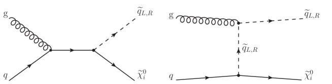
Figure 2: Feynman diagrams of the subprocess $q\text{g}\rightarrow\widetilde{\chi}_{i}^{0}\widetilde{q}_{L,R}$ to leading level.

The tree-level Feynman diagrams of the subprocess are displayed in Fig. 2. This subprocess receives $s$-channel contribution from exchange of quark, as well as $t$-channel contribution via exchange of the left- and right-handed squark $\widetilde{q}_{L,R}$. The leading-level contributions to the amplitude arising from the two diagrams in Fig. 2 are

$$T_{\hat{s}}=-\frac{\sqrt{2}g_{s}gT_{kj}^{l}}{\hat{s}c_{W}}\biggl{[}\overline{u}_{\widetilde{\chi}_{i}^{0}}(k_{1})(C_{\widetilde{\chi}_{i}^{0}\widetilde{q}q}^{L}P_{L}+C_{\widetilde{\chi}_{i}^{0}\widetilde{q}q}^{R}P_{R})(\not{p}_{1}+\not{p}_{2})\not{\epsilon}_{2}u(p_{1})\biggr{]},$$ (20)

$$T_{\hat{t}}=-\frac{\sqrt{2}g_{s}gT_{mj}^{l}}{c_{W}}\biggl{[}\overline{u}_{\widetilde{\chi}_{i}^{0}}(k_{1})\biggl{\{}\frac{C_{\widetilde{\chi}_{i}^{0}\widetilde{q}q}^{L}P_{L}}{(\hat{t}-m_{\widetilde{q}_{L}}^{2})}+\frac{C_{\widetilde{\chi}_{i}^{0}\widetilde{q}q}^{R}P_{R}}{(\hat{t}-m_{\widetilde{q}_{R}}^{2})}\biggr{\}}u(p_{1})\biggr{]}(2\epsilon_{2}\cdot k_{2}),$$ (21)

where $\epsilon_{2}$ denotes the polarization vector of the initial gluon. The relevant couplings are given in Eq. (5). After averaging over spins and colors in the initial state, the parton-level differential cross section for this subprocess takes the form

$$\frac{d\hat{\sigma}}{d\hat{t}}(q\text{g}\rightarrow\widetilde{\chi}_{i}^{0}\widetilde{q}_{L,R})=\frac{1}{1536\pi\hat{s}^{2}}\left(M_{\hat{s}\hat{s}}+M_{\hat{t}\hat{t}}+2M_{\hat{s}\hat{t}}\right),$$ (22)

where

$$M_{\hat{s}\hat{s}}=\frac{16g_{s}^{2}g^{2}}{\hat{s}^{2}c_{W}^{2}}\biggl{[}|C_{\widetilde{\chi}_{i}^{0}\widetilde{q}q}^{L}|^{2}+|C_{\widetilde{\chi}_{i}^{0}\widetilde{q}q}^{R}|^{2}\biggr{]}(m_{\widetilde{\chi}_{i}^{0}}^{2}-\hat{u})\hat{s},$$ (23)

$$M_{\hat{t}\hat{t}}=\frac{32g_{s}^{2}g^{2}}{c_{W}^{2}}\biggl{[}\frac{|C_{\widetilde{\chi}_{i}^{0}\widetilde{q}q}^{L}|^{2}m_{\widetilde{q}_{L}}^{2}}{(\hat{t}-m_{\widetilde{q}_{L}}^{2})^{2}}+\frac{|C_{\widetilde{\chi}_{i}^{0}\widetilde{q}q}^{R}|^{2}m_{\widetilde{q}_{R}}^{2}}{(\hat{t}-m_{\widetilde{q}_{R}}^{2})^{2}}\biggr{]}(\hat{t}-m_{\widetilde{\chi}_{i}^{0}}^{2}),$$ (24)

$$M_{\hat{s}\hat{t}}=\frac{8g_{s}^{2}g^{2}}{c_{W}^{2}}\biggl{[}\frac{|C_{\widetilde{\chi}_{i}^{0}\widetilde{q}q}^{L}|^{2}}{(\hat{t}-m_{\widetilde{q}_{L}}^{2})\hat{s}}+\frac{|C_{\widetilde{\chi}_{i}^{0}\widetilde{q}q}^{R}|^{2}}{(\hat{t}-m_{\widetilde{q}_{R}}^{2})\hat{s}}\biggr{]}\biggl{[}(m_{\widetilde{\chi}_{i}^{0}}^{2}-\hat{u})(m_{\widetilde{\chi}_{i}^{0}}^{2}-\hat{t})-\hat{s}(m_{\widetilde{\chi}_{i}^{0}}^{2}-\hat{t})-\hat{s}m_{\widetilde{\chi}_{i}^{0}}^{2}\biggr{]}.$$ (25)

II.3 The subprocess $\bm{q\bar{q}^{\prime}\rightarrow\widetilde{\chi}_{i}^{0}\widetilde{\chi}_{j}^{+}}$

The neutralino and chargino production, which can dominantly be produced by annihilation of quarks and antiquarks at hadron colliders as follows:

$$q(p_{1})\overline{q}^{\prime}(p_{2})\rightarrow\widetilde{\chi}_{i}^{0}(k_{1})\widetilde{\chi}_{j}^{+}(k_{2}),$$ (26)

where particle labels denote the corresponding four-momentum. The kinematic is defined in Eq. (3), with $m_{i}$ denoting the neutralino mass and $m_{j}$ the chargino mass. The neutralino-chargino production occurs via the Feynman diagrams shown in Fig. 3.

Figure 3: Feynman diagrams of the subprocess $u\overline{d}\rightarrow\widetilde{\chi}_{i}^{0}\widetilde{\chi}_{j}^{+}$ to leading level.

This subprocess proceeds at tree level via the vector boson $W^{+}$ exchange in the $s$-channel, and via $t$- and $u$-channel exchange of the left squark $\widetilde{u}_{L}$ and $\widetilde{d}_{L}$. The tree-level contributions to the amplitude arising from the three diagrams in Fig. 3 are

$$\begin{split}T_{\hat{s}}=-&\frac{g^{2}}{c_{W}^{2}}D_{W}(\hat{s})\biggl{[}\overline{u}_{i}(k_{1})\gamma_{\mu}\left(O^{L}_{ij}P_{L}+O^{R}_{ij}P_{R}\right){v}_{j}(k_{2})\biggr{]}\\ &\cdot\biggl{[}\overline{v}(p_{2})\gamma^{\mu}\left(L_{Wqq^{\prime}}P_{L}+R_{Wqq^{\prime}}P_{R}\right)u(p_{1})\biggr{]},\end{split}$$ (27)

$$\begin{split}T_{\hat{t}}=&\frac{2g^{2}}{(\hat{t}-m_{\widetilde{q}_{L}}^{2})c_{W}^{2}}\biggl{[}\overline{u}_{i}(k_{1})\left(C_{\widetilde{\chi}_{i}^{0}\widetilde{q}q}^{L*}P_{L}+C_{\widetilde{\chi}_{i}^{0}\widetilde{q}q}^{R*}P_{R}\right)u(p_{1})\biggr{]}\\ &\cdot\biggl{[}\overline{v}(p_{2})\gamma^{\mu}\left(C_{\widetilde{\chi}_{j}^{+}\widetilde{q}q^{\prime}}^{L}P_{L}+C_{\widetilde{\chi}_{j}^{+}\widetilde{q}q^{\prime}}^{R}P_{R}\right)v_{j}(k_{2})\biggr{]},\end{split}$$ (28)

$$\begin{split}T_{\hat{u}}=&\frac{2g^{2}}{(\hat{u}-m_{{\widetilde{q}}^{\prime}_{L}}^{2})c_{W}^{2}}\biggl{[}\overline{u}_{j}(k_{2})\left(C_{\widetilde{\chi}_{j}^{+}{\widetilde{q}}^{\prime}q}^{L*}P_{L}+C_{\widetilde{\chi}_{j}^{+}{\widetilde{q}}^{\prime}q}^{R*}P_{R}\right)u(p_{1})\biggr{]}\\ &\cdot\biggl{[}\overline{v}(p_{2})\gamma^{\mu}\left(C_{\widetilde{\chi}_{i}^{0}{\widetilde{q}}^{\prime}q^{\prime}}^{L}P_{L}+C_{\widetilde{\chi}_{i}^{0}{\widetilde{q}}^{\prime}q^{\prime}}^{R}P_{R}\right)v_{i}(k_{1})\biggr{]}.\end{split}$$ (29)

In order to obtain the cross section for this subprocess, one would have to calculate the couplings of the neutralino-quark-squark, chargino-quark-squark and neutralino-chargino-$W^{+}$ boson. We summarize these couplings in Eqs.(4)-(6). The analytic form of the partonic differential cross section after spin and color averaging reads

$$\frac{d\hat{\sigma}}{d\hat{t}}(q\overline{q}^{\prime}\rightarrow\widetilde{\chi}_{i}^{0}\widetilde{\chi}_{j}^{+})=\frac{1}{192\pi\hat{s}^{2}}\left(M_{\hat{s}\hat{s}}+M_{\hat{t}\hat{t}}+M_{\hat{u}\hat{u}}-2M_{\hat{s}\hat{t}}+2M_{\hat{s}\hat{u}}-2M_{\hat{t}\hat{u}}\right),$$ (30)

where

$$\begin{split}M_{\hat{s}\hat{s}}=&\frac{4g^{2}|D_{W}(\hat{s})|^{2}}{c_{W}^{4}}\biggl{\{}\biggl{[}L_{Wqq^{\prime}}^{2}+R_{Wqq^{\prime}}^{2}\biggr{]}\biggl{[}O^{L}_{ij}O^{R*}_{ij}+O^{L*}_{ij}O^{R}_{ij}\biggr{]}m_{\widetilde{\chi}_{i}^{0}}m_{\widetilde{\chi}_{j}^{+}}\hat{s}\\ &+\biggl{[}|O^{L}_{ij}|^{2}L_{Wqq^{\prime}}^{2}+|O^{R}_{ij}|^{2}R_{Wqq^{\prime}}^{2}\biggr{]}(m_{\widetilde{\chi}_{i}^{0}}^{2}-\hat{u})(m_{\widetilde{\chi}_{j}^{+}}^{2}-\hat{u})\\ &+\biggl{[}|O^{L}_{ij}|^{2}R_{Wqq^{\prime}}^{2}+|O^{R}_{ij}|^{2}L_{Wqq^{\prime}}^{2}\biggr{]}(m_{\widetilde{\chi}_{i}^{0}}^{2}-\hat{t})(m_{\widetilde{\chi}_{j}^{+}}^{2}-\hat{t})\biggr{\}},\end{split}$$ (31)

$$M_{\hat{t}\hat{t}}=\frac{4g^{2}}{(\hat{t}-m_{\widetilde{q}_{L}}^{2})^{2}c_{W}^{4}}\biggl{[}|C_{\widetilde{\chi}_{i}^{0}\widetilde{q}q}^{L}|^{2}+|C_{\widetilde{\chi}_{i}^{0}\widetilde{q}q}^{R}|^{2}\biggr{]}\biggl{[}|C_{\widetilde{\chi}_{j}^{+}\widetilde{q}q^{\prime}}^{L}|^{2}+|C_{\widetilde{\chi}_{j}^{+}\widetilde{q}q^{\prime}}^{R}|^{2}\biggr{]}(m_{\widetilde{\chi}_{i}^{0}}^{2}-\hat{t})(m_{\widetilde{\chi}_{j}^{+}}^{2}-\hat{t}),$$ (32)

$$M_{\hat{u}\hat{u}}=\frac{4g^{2}}{(\hat{u}-m_{\widetilde{q}^{\prime}_{L}}^{2})^{2}c_{W}^{4}}\biggl{[}|C_{\widetilde{\chi}_{j}^{+}\widetilde{q}^{\prime}q}^{L}|^{2}+|C_{\widetilde{\chi}_{j}^{+}\widetilde{q}^{\prime}q}^{R}|^{2}\biggr{]}\biggl{[}|C_{\widetilde{\chi}_{i}^{0}\widetilde{q}^{\prime}q^{\prime}}^{L}|^{2}+|C_{\widetilde{\chi}_{i}^{0}\widetilde{q}^{\prime}q^{\prime}}^{R}|^{2}\biggr{]}(m_{\widetilde{\chi}_{i}^{0}}^{2}-\hat{u})(m_{\widetilde{\chi}_{j}^{+}}^{2}-\hat{u}),$$ (33)

$$M_{\hat{t}\hat{u}}=\frac{4g^{2}}{(\hat{t}-{m}_{\widetilde{q}_{L}}^{2})(\hat{u}-m_{\widetilde{q}^{\prime}_{L}}^{2})c_{W}^{4}}\biggl{\{}\frac{1}{2}\left[C_{\widetilde{\chi}_{i}^{0}\widetilde{q}q}^{L*}C_{\widetilde{\chi}_{i}^{0}\widetilde{q}^{\prime}q^{\prime}}^{L*}C_{\widetilde{\chi}_{j}^{+}\widetilde{q}^{\prime}q}^{L}C_{\widetilde{\chi}_{j}^{+}\widetilde{q}q^{\prime}}^{L}+C_{\widetilde{\chi}_{i}^{0}\widetilde{q}q}^{R*}C_{\widetilde{\chi}_{i}^{0}\widetilde{q}^{\prime}q^{\prime}}^{R*}C_{\widetilde{\chi}_{j}^{+}\widetilde{q}^{\prime}q}^{R}C_{\widetilde{\chi}_{j}^{+}\widetilde{q}q^{\prime}}^{R}\right]$$

$$\times\left[(m_{\widetilde{\chi}_{i}^{0}}^{2}-\hat{u})(m_{\widetilde{\chi}_{j}^{+}}^{2}-\hat{u})+(m_{\widetilde{\chi}_{i}^{0}}^{2}-\hat{t})(m_{\widetilde{\chi}_{j}^{+}}^{2}-\hat{t})-\hat{s}(\hat{s}-m_{\widetilde{\chi}_{i}^{0}}^{2}-m_{\widetilde{\chi}_{j}^{+}}^{2})\right]$$ (34)

$$+m_{\widetilde{\chi}_{i}^{0}}m_{\widetilde{\chi}_{j}^{+}}\hat{s}\left[C_{\widetilde{\chi}_{i}^{0}\widetilde{q}q}^{L*}C_{\widetilde{\chi}_{i}^{0}\widetilde{q}^{\prime}q^{\prime}}^{R*}C_{\widetilde{\chi}_{j}^{+}\widetilde{q}^{\prime}q}^{L}C_{\widetilde{\chi}_{j}^{+}\widetilde{q}q^{\prime}}^{R}+C_{\widetilde{\chi}_{i}^{0}\widetilde{q}q}^{R*}C_{\widetilde{\chi}_{i}^{0}\widetilde{q}^{\prime}q^{\prime}}^{L*}C_{\widetilde{\chi}_{j}^{+}\widetilde{q}^{\prime}q}^{R}C_{\widetilde{\chi}_{j}^{+}\widetilde{q}q^{\prime}}^{L}\right]\biggr{\}},$$

$$M_{\hat{s}\hat{u}}=\frac{-4g^{4}(Re[D_{W}(\hat{s})])}{(\hat{u}-m_{\widetilde{q}^{\prime}_{L}}^{2})c_{W}^{4}}\biggl{\{}\left[L_{Wqq^{\prime}}O^{R}_{ij}C_{\widetilde{\chi}_{i}^{0}\widetilde{q}^{\prime}q^{\prime}}^{L*}C_{\widetilde{\chi}_{j}^{+}\widetilde{q}^{\prime}q}^{L}+R_{Wqq^{\prime}}O^{L}_{ij}C_{\widetilde{\chi}_{i}^{0}\widetilde{q}^{\prime}q^{\prime}}^{R*}C_{\widetilde{\chi}_{j}^{+}\widetilde{q}^{\prime}q}^{R}\right]\\$$

$$\times(m_{\widetilde{\chi}_{i}^{0}}^{2}-\hat{u})(m_{\widetilde{\chi}_{j}^{+}}^{2}-\hat{u})+m_{\widetilde{\chi}_{i}^{0}}m_{\widetilde{\chi}_{j}^{+}}\hat{s}\\$$ (35)

$$\times\left[L_{Wqq^{\prime}}O^{L}_{ij}C_{\widetilde{\chi}_{i}^{0}\widetilde{q}^{\prime}q^{\prime}}^{L*}C_{\widetilde{\chi}_{j}^{+}\widetilde{q}^{\prime}q}^{L}+R_{Wqq^{\prime}}O^{R}_{ij}C_{\widetilde{\chi}_{i}^{0}\widetilde{q}^{\prime}q^{\prime}}^{R*}C_{\widetilde{\chi}_{j}^{+}\widetilde{q}^{\prime}q}^{R}\right]\biggr{\}},$$

$$M_{\hat{s}\hat{t}}=\frac{-4g^{4}(Re[D_{W}(\hat{s})])}{(\hat{t}-m_{\widetilde{q}_{L}}^{2})c_{W}^{4}}\biggl{\{}\left[L_{Wqq^{\prime}}O^{R}_{ij}C_{\widetilde{\chi}_{i}^{0}\widetilde{q}q}^{L}C_{\widetilde{\chi}_{j}^{+}\widetilde{q}q^{\prime}}^{L*}+R_{Wqq^{\prime}}O^{L}_{ij}C_{\widetilde{\chi}_{i}^{0}\widetilde{q}q}^{R}C_{\widetilde{\chi}_{j}^{+}\widetilde{q}q^{\prime}}^{R*}\right]\\$$

$$\times(m_{\widetilde{\chi}_{i}^{0}}^{2}-\hat{t})(m_{\widetilde{\chi}_{j}^{+}}^{2}-\hat{t})+m_{\widetilde{\chi}_{i}^{0}}m_{\widetilde{\chi}_{j}^{+}}\hat{s}\\$$ (36)

$$\times\left[L_{Wqq^{\prime}}O^{L}_{ij}C_{\widetilde{\chi}_{i}^{0}\widetilde{q}q}^{L}C_{\widetilde{\chi}_{j}^{+}\widetilde{q}q^{\prime}}^{L*}+R_{Wqq^{\prime}}O^{R}_{ij}C_{\widetilde{\chi}_{i}^{0}\widetilde{q}q}^{R}C_{\widetilde{\chi}_{j}^{+}\widetilde{q}q^{\prime}}^{R*}\right]\biggr{\}}.$$

In the above relations, the following abbreviation has been used $D_{W}(\hat{s})=\frac{1}{\hat{s}-m_{W}^{2}+im_{W}\Gamma_{W}}$, which is the $W$-boson propagator denominator. We get $m_{W}$ = 80.385 GeV and the width of this boson is $\Gamma_{W}=2.085$ GeV for calculations.

II.4 The subprocess $\bm{\text{g}\text{g}\rightarrow\widetilde{\chi}_{i}^{0}\widetilde{\text{g}}}$

The associated production of neutralino and gluino can be produced via the collision of gluon-gluon as follows:

$$\text{g}^{k}(p_{1})\text{g}^{l}(p_{2})\rightarrow\widetilde{\chi}_{i}^{0}(k_{1})\widetilde{\text{g}}^{m}(k_{2}),$$ (37)

where $p_{1}$ and $p_{2}$ denote the four-momentum of the initial gluons, and $k_{1}$ and $k_{2}$ represent the four-momentum of the two final-state neutralino and gluino, respectively. We denote by $k,l$ and $m$ the color indices of gluons and gluino, respectively. This subprocess first emerges at the one-loop level. We have performed the numerical evaluation for the subprocess $\text{g}\text{g}\to\widetilde{\chi}_{i}^{0}\widetilde{\text{g}}$ at one-loop using the Mathematica packages FeynArts Feynarts to calculate corresponding amplitudes, FormCalc Hahn ; Hahn2 to produce a complete Fortran code containing the squared matrix elements, and LoopTools loop to perform the evaluation of the necessary loop integrals. Also, the Feynman diagrams depicted in Fig. 4 have been generated by using FeynArts. In general, the one-loop corrections to subprocess $\text{g}\text{g}\rightarrow\widetilde{\chi}_{i}^{0}\widetilde{\text{g}}$ could be classified as vertex contributions and box contributions.

Figure 4: Feynman diagrams of the subprocess $\text{g}\text{g}\rightarrow\widetilde{\chi}_{i}^{0}\widetilde{\text{g}}$ to one-loop level. Also, this subprocess contains diagrams which are obtained by the replacements $u_{m}\rightarrow d_{m}$ and $\widetilde{u}_{m}^{w}\rightarrow\widetilde{d}_{m}^{w}$ in the above diagrams. Here, m and w indices denote the generation of (s)quark and the mass eigenstate of squark, respectively.

The calculations of this subprocess have been carried out in the ’t Hooft-Feynman gauge in which the gluon polarization sum is $\sum_{\lambda}\epsilon_{\mu}^{*}(k,\lambda)\epsilon_{\nu}(k,\lambda)=-g_{\mu\nu}$. For regularization of the ultraviolet divergences, we have used the constrained differential renormalization (CDR) CDR , which has been shown to be equivalent to regularization by dimensional reduction DR ; DR2 at the one-loop level. Therefore, a supersymmetry-preserving regularization scheme is ensured via the implementation given in Ref. DR3 . We do not display the analytical results of this process due to the fact that these are too long to be included here.

III Numerical analysis and discussions

We now present numerical predictions for the cross sections of the single neutralino production in $pp$ collisions at the LHC energies. We investigate the direct production of a single neutralino $\widetilde{\chi}_{i}^{0}$ for first-generation quarks at hadron colliders focusing on the $\widetilde{\chi}_{1}^{0}$ is likely to be the LSP and $\widetilde{\chi}_{2}^{0}$. The relevant subprocesses are $q\bar{q}\to\widetilde{\chi}_{i}^{0}\widetilde{\text{g}}$, $q\text{g}\to\widetilde{\chi}_{i}^{0}\widetilde{q}_{L,R}$ and $q\bar{q}^{\prime}\to\widetilde{\chi}_{i}^{0}\widetilde{\chi}_{j}^{\pm}$ at tree-level, while $\text{g}\text{g}\to\widetilde{\chi}_{i}^{0}\widetilde{\text{g}}$ at one-loop level, which could lead to the first detection of the supersymmetric particles at the LHC. In the numerical calculations, we just limit the values of the mass parameters $M_{1}$, $M_{2}$ and $\mu$ to be real, positive and below 1 TeV, and get $\tan\beta$= 45, $m_{\widetilde{u}_{R}}$= 799.2 GeV, $m_{\widetilde{u}_{L}}$= 798.2 GeV, $m_{\widetilde{d}_{R}}$= 802.3 GeV, $m_{\widetilde{d}_{L}}$= 800.3 GeV and $m_{\widetilde{g}}$= 1400 GeV. For the other parameters, we use the values given by the Particle Data Group, such as $m_{Z}$= 91.1876 GeV, $m_{W}$= 80.399 GeV PDG . By using Eqs. (50) and (51) with two chargino masses, one could have three choices of parameter sets for the gaugino/Higgsino mass parameters $M_{2}$ and $\mu$ in three different cases, which are the gaugino-like, the higgsino-like and the mixture-case, respectively. We fix masses of the charginos as $m_{\widetilde{\chi}_{1}^{\pm}}=168.51$ GeV and $m_{\widetilde{\chi}_{2}^{\pm}}=295.01$ GeV for gaugino and higgsino-like scenarios, and $m_{\widetilde{\chi}_{1}^{\pm}}=173.66$ GeV and $m_{\widetilde{\chi}_{2}^{\pm}}=289.86$ GeV for mixture-case. For each scenario, neutralino masses are calculated by inserting the values of $M_{2}$ and $\mu$ into Eq. (45). Table 1 shows the gaugino/Higgsino and neutralino masses.

Table 1: The gaugino/Higgsino mass parameters and neutralino masses for each scenario.

[in GeV]	$M_{2}$	$\mu$	$M_{1}$	$m_{\widetilde{\chi}_{1}^{0}}$	$m_{\widetilde{\chi}_{2}^{0}}$	$m_{\widetilde{\chi}_{3}^{0}}$	$m_{\widetilde{\chi}_{4}^{0}}$
Higgsino like	250.00	200.00	119.33	109.59	174.50	209.65	294.88
Gaugino like	200	250.00	95.46	91.50	169.50	259.40	293.85
Mixture case	225.00	225.00	107.39	101.42	176.13	234.52	289.37
CMSSM 40.2.2	391.24	698.59	210.84	208.23	397.26	702.97	711.31

For comparison, we have also worked out the cross sections in the CMSSM 40.2.2 benchmark point CMSSM4022 in the framework of the CMSSM CMSSM ; CMSSM2 ; CMSSM3 with five input parameters, namely, $m_{0}=$ 600 GeV, $m_{1/2}=$ 500 GeV, $A_{0}=-$ 500 GeV, $\tan\beta=$ 40 and $\mu>0$, where the parameters $m_{0}$ and $m_{1/2}$ are the universal scalar and gaugino mass parameters, $A_{0}$ is the universal trilinear soft SUSY breaking parameter, $\tan\beta$ is the ratio of the vacuum expectation values of the two Higgs doublets and sign($\mu$) is the sign of the Higgs mixing parameter. The universal parameters $m_{0}$, $m_{1/2}$ and $A_{0}$ are thought to appear by means of some gravity-mediated mechanism and are defined at the grand unified theories scale, whereas $\tan\beta$ and sign of the Higgs mixing parameter sign($\mu$) are defined at the electroweak scale. All the masses and couplings of the model from these five parameters are obtained by the evolution from the grand unified theories scale down to the electroweak scale Drees . In this case, we have computed the SUSY particle spectrum by using SoftSusy-3.3.4 package softsusy . For the CMSSM 40.2.2 benchmark point, the gaugino masses $M_{2}$ and $M_{1}$, the Higgsino mass $\mu$, and neutralino masses are given in Table 1, and the other parameters are obtained as $m_{\widetilde{\chi}_{1}^{+}}=397.33$ GeV, $m_{\widetilde{\chi}_{2}^{+}}=711.85$ GeV, $m_{\widetilde{u}_{L}}=1199.95$ GeV, $m_{\widetilde{d}_{L}}=1202.41$ GeV, $m_{\widetilde{u}_{R}}=1167.94$ GeV, $m_{\widetilde{d}_{R}}=1165.21$ GeV, and $m_{\widetilde{\text{g}}}=1170.38$ GeV.

We use the MSTW2008 parton distribution functions MSTW for the quark/gluon distributions inside the proton and fix the renormalization and factorization scales to the average final-state mass in our numerical calculations. For each scenario given above, we have numerically evaluated the hadronic cross sections of the single neutralino production processes involving a neutralino $\widetilde{\chi}_{1}^{0}$ or $\widetilde{\chi}_{2}^{0}$ in the final state, as a function of the center-of-mass energy from Figs. 5 to 8, the $M_{2}$-$\mu$ mass plane from Figs. 9 to 12, the squark mass from Figs. 13 to 16, and $\tan\beta$ from Figs. 17 to 20. In some of the figures, we use abbreviations as follows: higgsino-like $\rightarrow$ HL(solid line), gaugino-like $\rightarrow$ GL(dashed line), mixture-case $\rightarrow$ MC(dotted-line) and CMSSM 40.2.2 benchmark point $\rightarrow$ CMSSM(dot-dashed line), respectively. We now offer the following analysis of these figures in detail, separately.

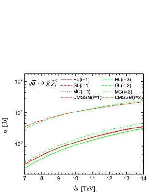
Figure 5: (color online). Total cross sections of the process $pp\to\widetilde{\text{g}}\widetilde{\chi}_{i}^{0}$ (i=1,2) versus the center-of-mass energy of $pp$ collider $\sqrt{s}$.

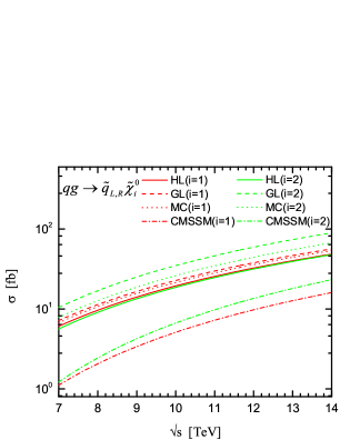
Figure 6: (color online). Total cross sections for the process $pp\to\widetilde{q}_{L,R}\widetilde{\chi}_{i}^{0}$ (i=1,2) versus the center-of-mass energy of $pp$ collider $\sqrt{s}$.

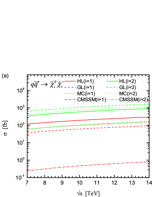
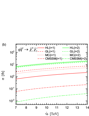
Figure 7: (color online). Total cross sections of the processes $pp\to\widetilde{\chi}_{i}^{0}\widetilde{\chi}_{1}^{+}$ (left) and $\widetilde{\chi}_{i}^{0}\widetilde{\chi}_{2}^{+}$ (right) (i=1,2) versus the center-of-mass energy of $pp$ collider $\sqrt{s}$.

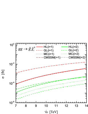
Figure 8: (color online). Total cross sections of the process $pp(\text{g}\text{g})\to\widetilde{\text{g}}\widetilde{\chi}_{i}^{0}$ (i=1,2) versus the center-of-mass energy of $pp$ collider $\sqrt{s}$.

In Figs. 5, 6, 7 and 8, we plot the dependence of the total cross sections for the single neutralino processes of the center-of-mass energy. These figures indicate that the total cross sections increase slowly and smoothly with increasing the beam energy from 7 TeV to 14 TeV for each scenario. The CMSSM 40.2.2 benchmark point and gaugino-like scenario are dominant for $pp\rightarrow\widetilde{\chi}_{i}^{0}\widetilde{\text{g}}$ and $pp\rightarrow\widetilde{\chi}_{i}^{0}\widetilde{q}_{L,R}$, respectively; however, in the associated production of a chargino with $\widetilde{\chi}_{i}^{0}$, these dominancies vary such that the gaugino-like scenario is dominant for $pp\to\widetilde{\chi}_{1}^{+}\widetilde{\chi}_{2}^{0}$ and $\widetilde{\chi}_{2}^{+}\widetilde{\chi}_{1}^{0}$ while the higgsino-like and mixture-case scenarios are dominant for $pp\to\widetilde{\chi}_{1}^{+}\widetilde{\chi}_{1}^{0}$ and $\widetilde{\chi}_{2}^{+}\widetilde{\chi}_{2}^{0}$ because of contributions to cross section from not only neutralino mixing matrix but also chargino mixing matrixes. The difference of the cross sections in scenarios comes only from the change of the couplings given in Eqs. (4)-(6) where the mixing matrices are changed. For cross sections of the process $\text{g}\text{g}\to\widetilde{\chi}_{i}^{0}\widetilde{\text{g}}$ at one-loop, higgsino-like scenario is larger than other scenarios. As shown in Fig. 5, the cross section of the process $pp\to\widetilde{\chi}_{1}^{0}\widetilde{\text{g}}$ in the CMSSM 40.2.2 benchmark point is about 9 times larger than in the gaugino-like, higgsino-like and mixture-case scenarios. Also, the cross section of the process $pp\to\widetilde{\chi}_{2}^{0}\widetilde{\text{g}}$ in the the CMSSM 40.2.2 benchmark point is 7, 9 and 11 times larger than in the gaugino-like, mixture-case and higgsino-like scenarios, respectively. As seen from Fig. 6, the cross section of the process $pp\to\widetilde{\chi}_{1}^{0}\widetilde{q}_{L,R}$ in the gaugino-like scenarios is about 17%, 6%, and 4 times larger than in the higgsino-like scenario, mixture-case scenario and CMSSM 40.2.2 benchmark point, respectively. Also, the cross section of the process $pp\to\widetilde{\chi}_{2}^{0}\widetilde{q}_{L,R}$ in the gaugino-like scenario is 87%, 34% and 5 times larger than in the higgsino-like scenario, mixture-case scenarios and CMSSM 40.2.2 benchmark point, respectively. It can be seen from in Fig. 7(a) that the cross section of the process $pp\to\widetilde{\chi}_{1}^{0}\widetilde{\chi}_{1}^{+}$ in the higgsino-like scenario is 3.2 times, 96% and 3 orders of magnitude larger than in the gaugino-like scenario, mixture-case scenario and CMSSM 40.2.2 benchmark point, respectively. The cross section of the process $pp\to\widetilde{\chi}_{2}^{0}\widetilde{\chi}_{1}^{+}$ in the gaugino-like scenario is roughly 2 times, 44% and 1 orders of magnitude larger than in the higgsino-like scenario, mixture-case scenario and CMSSM 40.2.2 benchmark point, respectively. Also, as shown in Fig. 7(b), the cross section of the process $pp\to\widetilde{\chi}_{1}^{0}\widetilde{\chi}_{2}^{+}$ in the gaugino-like scenario is roughly 3.6 times, 1.4 times and 1 orders of magnitude larger than in the higgsino-like scenario, mixture-case scenario and CMSSM 40.2.2 benchmark point, respectively. The cross section of the process $pp\to\widetilde{\chi}_{2}^{0}\widetilde{\chi}_{2}^{+}$ in the mixture-case scenario is roughly 11%, 27% and 3 orders of magnitude larger than in the higgsino-like scenario, in the gaugino-like scenario and the CMSSM 40.2.2 benchmark point, respectively. As shown in Fig. 8, the cross section of the process $\text{g}\text{g}\to\widetilde{\chi}_{1}^{0}\widetilde{\text{g}}$ in the CMSSM 40.2.2 benchmark point is about 7.4, 7.1 and 7 times larger than in the gaugino-like scenario, higgsino-like scenario and mixture-case scenario, respectively. The cross section for $\text{g}\text{g}\to\widetilde{\chi}_{2}^{0}\widetilde{\text{g}}$ in the CMSSM 40.2.2 benchmark point is about 6.7 times, 2.8 times and 10% larger than in the gaugino-like scenario, mixture-case scenario and higgsino-like scenario, respectively.

Table 2: Total cross sections (in fb) for the single neutralino production at center-of-mass energy $\sqrt{s}=$ 7 and 14 TeV.

	Higgsino like		Gaugino like		Mixture case		CMSSM 40.2.2
$\sigma$(process) [fb]	7 TeV	14 TeV	7 TeV	14 TeV	7 TeV	14 TeV	7 TeV	14 TeV
$\sigma(pp\to\widetilde{\chi}_{1}^{0}\widetilde{\text{g}})$	0.22	3.70	0.22	3.61	0.23	3.75	3.66	22.44
$\sigma(pp\to\widetilde{\chi}_{2}^{0}\widetilde{\text{g}})$	0.17	3.13	0.25	4.80	0.21	3.97	3.15	24.79
$\sigma(pp\to\widetilde{\chi}_{1}^{0}\widetilde{q}_{L,R})$	6.07	48.66	7.18	56.59	6.75	53.67	1.11	16.07
$\sigma(pp\to\widetilde{\chi}_{2}^{0}\widetilde{q}_{L,R})$	5.63	47.82	10.50	89.95	7.84	67.33	1.22	23.31
$\sigma(pp\to\widetilde{\chi}_{1}^{0}\widetilde{\chi}_{1}^{+})~{}~{}$	117.92	296.75	37.83	93.53	60.10	150.75	0.24	0.80
$\sigma(pp\to\widetilde{\chi}_{2}^{0}\widetilde{\chi}_{1}^{+})~{}~{}$	346.94	922.03	629.53	1654.78	434.16	1157.26	59.10	163.32
$\sigma(pp\to\widetilde{\chi}_{1}^{0}\widetilde{\chi}_{2}^{+})~{}~{}$	0.64	2.24	2.56	7.67	1.78	5.52	0.06	0.22
$\sigma(pp\to\widetilde{\chi}_{2}^{0}\widetilde{\chi}_{2}^{+})~{}~{}$	6.54	19.11	5.78	16.64	7.31	21.11	0.01	0.04
$\sigma(pp\to\widetilde{\chi}_{1}^{0}\widetilde{\text{g}})_{\text{one-loop}}$	$\mathscr{O}(10^{-4})$	$\mathscr{O}(10^{-3})$	$\mathscr{O}(10^{-4})$	$\mathscr{O}(10^{-3})$	$\mathscr{O}(10^{-4})$	$\mathscr{O}(10^{-3})$	$\mathscr{O}(10^{-3})$	0.02
$\sigma(pp\to\widetilde{\chi}_{2}^{0}\widetilde{\text{g}})_{\text{one-loop}}$	$\mathscr{O}(10^{-5})$	$\mathscr{O}(10^{-4})$	$\mathscr{O}(10^{-6})$	$\mathscr{O}(10^{-4})$	$\mathscr{O}(10^{-6})$	$\mathscr{O}(10^{-4})$	$\mathscr{O}(10^{-5})$	$\mathscr{O}(10^{-4})$

In Table 2, the cross sections of single neutralino associated production at center-of-mass energy $\sqrt{s}=$ 7 TeV and 14 TeV are given for each scenario. It is clear from this table that the cross section of the process $pp\to\widetilde{\chi}_{2}^{0}\widetilde{\chi}_{1}^{+}$ in the gaugino-like scenario yields cross sections of $\thicksim$600 to 1700 fb for $\sqrt{s}=$ 7 TeV and 14 TeV, which is larger than the remaining ones. Moreover, the cross section for $pp\to\widetilde{\chi}_{1}^{0}\widetilde{q}_{L,R}(\widetilde{\chi}_{2}^{0}\widetilde{q}_{L,R})$ reaches about 57(90) fb at $\sqrt{s}=$ 14 TeV in the gaugino-like. However, the process $pp(\text{g}\text{g})\to\widetilde{\chi}_{i}^{0}\widetilde{\text{g}}$ is suppressed by the others. The magnitudes of the cross sections are at a visible level of $10^{0}$ fb for $pp\rightarrow\widetilde{\chi}_{i}^{0}\widetilde{\text{g}}$, $10^{1}$ fb for $pp\rightarrow\widetilde{\chi}_{i}^{0}\widetilde{q}_{L,R}$, $10^{-1}$-$10^{3}$ fb for $pp\rightarrow\widetilde{\chi}_{i}^{0}\widetilde{\chi}_{j}^{+}$, and $10^{-4}$-$10^{-2}$ fb for $pp(\text{g}\text{g})\rightarrow\widetilde{\chi}_{i}^{0}\widetilde{\text{g}}$ at $\sqrt{s}=$ 14 TeV. Additionally, it can be easily seen that the cross section for the associated production of the next-to-lightest neutralino $\widetilde{\chi}_{2}^{0}$ is generally much larger than the cross section for associated production the lightest neutralino $\widetilde{\chi}_{1}^{0}$ for each scenario.

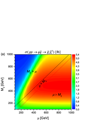
Figure 9: (color online). Contour plots of the total cross sections of the process $pp\to\widetilde{\text{g}}\widetilde{\chi}_{i}^{0}$ (i=1,2) in the $M_{2}-\mu$ plane for $\sqrt{s}=8$ TeV. We choose $\tan\beta=45$ and fix $M_{1}=\frac{5}{3}M_{2}\tan^{2}\theta_{W}$.

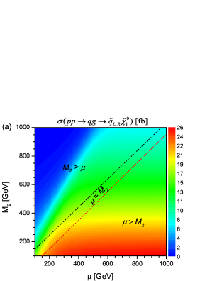
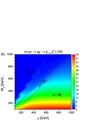
Figure 10: (color online). Contour plots of the total cross sections of the process $pp\to\widetilde{q}_{L,R}\widetilde{\chi}_{i}^{0}$ (i=1,2) in the $M_{2}-\mu$ plane for $\sqrt{s}=8$ TeV. We choose $\tan\beta=45$ and fix $M_{1}=\frac{5}{3}M_{2}\tan^{2}\theta_{W}$.

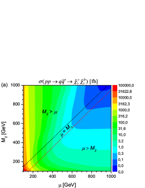
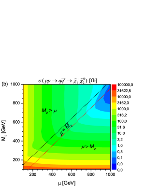
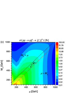
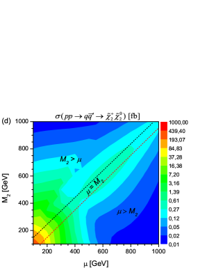
Figure 11: (color online). Contour plots of the total cross sections of the process $pp\to\widetilde{\chi}_{i}^{0}\widetilde{\chi}_{j}^{+}$ (i,j=1,2) in the $M_{2}-\mu$ plane for $\sqrt{s}=8$ TeV. We choose $\tan\beta=45$ and fix $M_{1}=\frac{5}{3}M_{2}\tan^{2}\theta_{W}$.

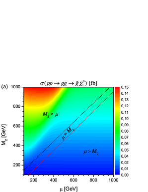
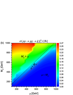
Figure 12: (color online). Contour plots of the total cross sections of the process $pp(\text{g}\text{g})\to\widetilde{\text{g}}\widetilde{\chi}_{i}^{0}$ (i=1,2) in the $M_{2}-\mu$ plane for $\sqrt{s}=8$ TeV. We choose $\tan\beta=45$ and fix $M_{1}=\frac{5}{3}M_{2}\tan^{2}\theta_{W}$.

The masses and mixing matrices of neutralino/chargino depend on the parameters $M_{2}$ and $\mu$; therefore, it is so important to study the dependence of the cross section of the single neutralino production on these parameters. Accordingly, we plot the dependence of the total cross section of the associated process in the $M_{2}$-$\mu$ mass plane with varying $M_{2}$ and $\mu$ in the range from 100 to 1000 GeV in steps of 50 GeV at center-of-mass energy 8 TeV for $\tan\beta=$ 45, as shown in Figs. 9, 10, 11 and 12. In these figures, the region above the black dashed-line corresponds to $M_{2}>\mu$ (higgsino-like) , the region below the red dashed-line corresponds to $M_{2}<\mu$ (gaugino-like) and the region between the two dashed lines corresponds to $\mu=M_{2}$ (mixture-case). One can note that these figures reconfirm the dominant scenarios which appear in the dependence of the cross sections on the center-of-mass energy. We can see from Figs. 9 and 10 that the cross sections of the processes $pp\rightarrow\widetilde{\chi}_{i}^{0}\widetilde{\text{g}}$ and $pp\rightarrow\widetilde{\chi}_{i}^{0}\widetilde{q}_{L,R}$ in the $M_{2}$-$\mu$ mass plane increase during both increasing $\mu$ and decreasing $M_{2}$. In particular, the maximum values are obtained in the region 200 $\lesssim\mu\lesssim$ 1000 GeV and $M_{2}\lesssim$ 400 GeV into the scan region. This case corresponds to the gaugino-like scenario. As a result, one can note that the cross section of these processes can be measured experimentally in some scenarios for a lower value of $M_{2}$. However, as illustrated in Fig. 11, the cross sections for $pp\to\widetilde{\chi}_{i}^{0}\widetilde{\chi}_{j}^{+}$ in the $M_{2}$-$\mu$ mass plane increase during both decreasing $\mu$ and $M_{2}$. Here, the maximum values are obtained in the region $\mu\lesssim$ 400 GeV and any value of $M_{2}$ for processes $pp\to\widetilde{\chi}_{1}^{0}\widetilde{\chi}_{1}^{+}$ ($M_{2}>\mu$) and $\widetilde{\chi}_{2}^{0}\widetilde{\chi}_{1}^{+}$ ($\mu>M_{2}$), while in the region 100 $\lesssim M_{2}\lesssim$ 400 GeV and 100 $\lesssim\mu\lesssim$ 400 GeV for processes $pp\to\widetilde{\chi}_{1}^{0}\widetilde{\chi}_{2}^{+}$ ($\mu>M_{2}$) and $\widetilde{\chi}_{2}^{0}\widetilde{\chi}_{2}^{+}$ ($\mu=M_{2}$). Note that, as mentioned before, the process of contributions to cross section from not only neutralino mixing matrix, but also chargino mixing matrixes. One can see from Fig. 12 that the dependence of the cross section of the process $\text{g}\text{g}\to\widetilde{\chi}_{i}^{0}\widetilde{\text{g}}$ in the $M_{2}$-$\mu$ mass plane increases with increasing $M_{2}$ and any value of $\mu$. In particular, the cross section of process $\text{g}\text{g}\to\widetilde{\chi}_{i}^{0}\widetilde{\text{g}}$ indicates the maximum values in the region 600 $\lesssim M_{2}\lesssim$ 1000 GeV and $\mu\lesssim$ 600 GeV as illustrated in Figs. 12(a) and 12(b). This case corresponds to higgsino-like scenario ($M_{2}>\mu$).

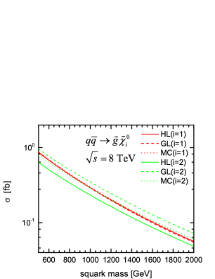
Figure 13: (color online). Total cross sections for the process $pp\to\widetilde{\text{g}}\widetilde{\chi}_{i}^{0}$ (i=1,2) depending on the squark mass at $\sqrt{s}=8$ TeV.

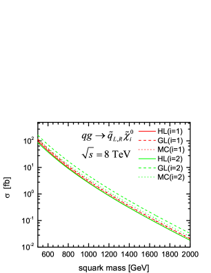
Figure 14: (color online). Total cross sections of the process $pp\to\widetilde{q}_{L,R}\widetilde{\chi}_{i}^{0}$ (i=1,2) depending on the squark mass at $\sqrt{s}=8$ TeV.

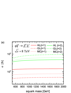
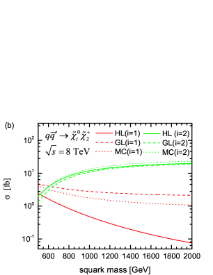
Figure 15: (color online). Total cross sections of the processes $pp\to\widetilde{\chi}_{i}^{0}\widetilde{\chi}_{1}^{+}$ (left) and $\widetilde{\chi}_{i}^{0}\widetilde{\chi}_{2}^{+}$ (right) (i=1,2) depending on the squark mass at $\sqrt{s}=8$ TeV.

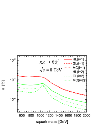
Figure 16: (color online). Total cross sections of the process $pp(\text{g}\text{g})\to\widetilde{\text{g}}\widetilde{\chi}_{i}^{0}$ (i=1,2) depending on the squark mass at $\sqrt{s}=8$ TeV.

In Figs. 13, 14, 15 and 16 we present the cross section as a function of squark mass for single neutralino production at $\sqrt{s}=$ 8 TeV. The total cross section for the single neutralino production processes apart from $pp\to\widetilde{\chi}_{i}^{0}\widetilde{\chi}_{j}^{+}$ are essentially determined by the squark masses so that it decreases with increasing the squark mass between 500 and 2000 GeV for each scenario. When the squark mass increases by a factor of 4, the cross section is pulled down by about 1, 3 and 2 orders of magnitude for the processes $pp\rightarrow\widetilde{\chi}_{i}^{0}\widetilde{\text{g}}$, $pp\rightarrow\widetilde{\chi}_{i}^{0}\widetilde{q}_{L,R}$ and $pp(\text{g}\text{g})\to\widetilde{\chi}_{i}^{0}\widetilde{\text{g}}$, respectively. On the other hand, for the process $pp\to\widetilde{\chi}_{i}^{0}\widetilde{\chi}_{j}^{+}$, the cross section is less affected with respect to variation in the squark mass because the s-channel of this process is dominant and together t- and u-channel terms are suppressed for large squark masses. The cross sections of the single neutralino production for the squark mass 1 and 2 TeV at $\sqrt{s}=$ 8 TeV so as to facilitate precise comparisons with the experimental results are summarized in Table 3. As seen from this table, the dependence of cross section on the squark mass is dominated by one of the processes, $pp\to\widetilde{\chi}_{2}^{0}\widetilde{\chi}_{1}^{+}$ appears 0.95 pb for the squark mass 2 TeV in the gaugino-like scenario.

Table 3: Total cross sections (in fb) for the single neutralino production processes in a function of the squark mass at $\sqrt{s}=$ 8 TeV.

	$m_{\widetilde{q}}$ [GeV]	$\widetilde{\chi}_{1}^{0}\widetilde{\text{g}}$	$\widetilde{\chi}_{2}^{0}\widetilde{\text{g}}$	$\widetilde{\chi}_{1}^{0}\widetilde{q}$	$\widetilde{\chi}_{2}^{0}\widetilde{q}$	$\widetilde{\chi}_{1}^{0}\widetilde{\chi}_{1}^{+}$	$\widetilde{\chi}_{2}^{0}\widetilde{\chi}_{1}^{+}$	$\widetilde{\chi}_{1}^{0}\widetilde{\chi}_{2}^{+}$	$\widetilde{\chi}_{2}^{0}\widetilde{\chi}_{2}^{+}$	$~{}\widetilde{\chi}_{1}^{0}\widetilde{\text{g}}_{\text{one-loop}}$	$\widetilde{\chi}_{2}^{0}\widetilde{\text{g}}_{\text{one-loop}}$
HL	1000	0.29	0.23	2.72	2.62	144.90	447.40	0.48	11.85	2.07$\cdot 10^{-5}$	4.16$\cdot 10^{-6}$
	2000	0.06	0.05	0.02	0.02	148.73	484.43	0.08	19.92	2.61$\cdot 10^{-7}$	4.93$\cdot 10^{-8}$
GL	1000	0.29	0.35	3.19	4.87	46.78	838.21	2.79	10.86	1.95$\cdot 10^{-5}$	1.96$\cdot 10^{-6}$
	2000	0.05	0.07	0.02	0.03	49.01	954.97	2.13	18.99	2.36$\cdot 10^{-7}$	0.86$\cdot 10^{-8}$
MC	1000	0.30	0.29	3.01	3.65	74.26	573.41	1.77	13.53	2.08$\cdot 10^{-5}$	2.45$\cdot 10^{-6}$
	2000	0.06	0.06	0.02	0.03	77.10	642.44	1.07	23.31	2.57$\cdot 10^{-7}$	2.02$\cdot 10^{-8}$

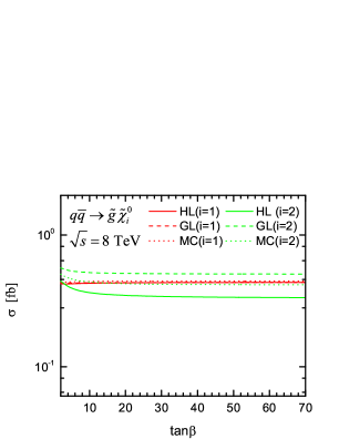
Figure 17: (color online). Total cross sections of the process $pp\to\widetilde{\text{g}}\widetilde{\chi}_{i}^{0}$ (i=1,2) as a function of $\tan{\beta}$ at $\sqrt{s}=8$ TeV.

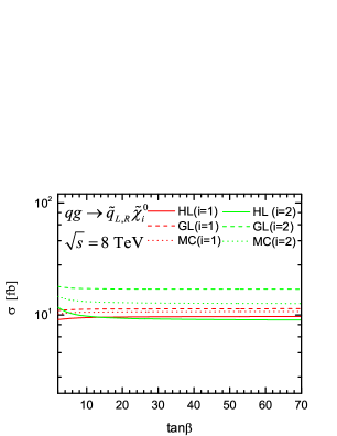
Figure 18: (color online). Total cross sections of the process $pp\to\widetilde{q}_{L,R}\widetilde{\chi}_{i}^{0}$ (i=1,2) as a function of $\tan{\beta}$ at $\sqrt{s}=8$ TeV.

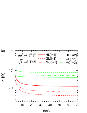
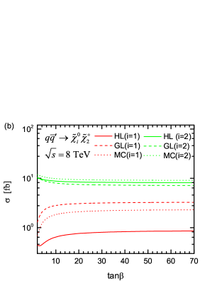
Figure 19: (color online). Total cross sections of the processes $pp\to\widetilde{\chi}_{i}^{0}\widetilde{\chi}_{1}^{+}$ (left) and $\widetilde{\chi}_{i}^{0}\widetilde{\chi}_{2}^{+}$ (right) (i=1,2) as a function of $\tan{\beta}$ at $\sqrt{s}=8$ TeV.

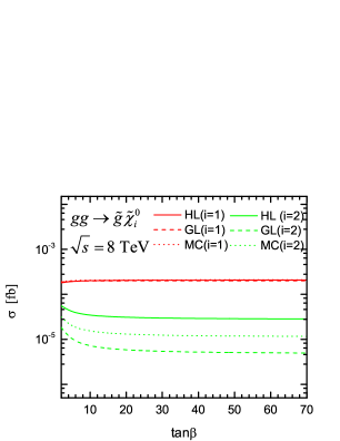
Figure 20: (color online). Total cross sections of the process $pp(\text{g}\text{g})\to\widetilde{\text{g}}\widetilde{\chi}_{i}^{0}$ (i=1,2) as a function of $\tan{\beta}$ at $\sqrt{s}=8$ TeV.

Finally, the $\tan\beta$ dependence of the cross sections for the single neutralino processes are depicted in Figs. 17, 18, 19 and 20. From these figures we can clearly see that cross sections of the processes $pp\to\widetilde{\chi}_{i}^{0}\widetilde{\text{g}}$, $pp\to\widetilde{\chi}_{i}^{0}\widetilde{q}_{L,R}$ and $\text{g}\text{g}\to\widetilde{\chi}_{i}^{0}\widetilde{\text{g}}$ increase (decrease) slowly for $i=1$ ($i=2$) when $\tan\beta$ goes up from 2 to 10, and vary smoothly when $\tan\beta>$ 10 for each scenario. However, the cross sections of the processes $pp\to\widetilde{\chi}_{i}^{0}\widetilde{\chi}_{j}^{+}$ apart from $pp\to\widetilde{\chi}_{1}^{0}\widetilde{\chi}_{2}^{+}$ decrease with increasing the $\tan\beta$ from 2 to 70. Moreover, there appear the same dominant scenarios as in the dependence of the cross sections on the center-of-mass energy.

The possible contributions to the background in the signal regions come from the Standard Model processes, as $pp\to WW$, $pp\to ZZ$, $pp\to WZ$ and $pp\to t\bar{t}$. If we are interested in signals with leptons in the final state, then in the case of $1l+\not{E}_{T}+jets$ mode, the background appears from $pp\to WW$, $pp\to WZ$ and $pp\to t\bar{t}$. Also, the processes $pp\to ZZ$, $pp\to WW$, and $pp\to t\bar{t}$ can yield background for the $2l+\not{E}_{T}+jets$ mode. The process $pp\to WZ$ can yield background for the $3l+\not{E}_{T}+0jets$ decay mode. Of course, all background channels could have large cross sections, but despite this it needs some additional cutoff mechanism that will help for the extraction, as mentioned above. An analysis of our calculations is shown since those background channels can have large cross sections. It should be noted that, in our case, the background cross section is about 1-3 orders of magnitude larger than the signal. We hope the at $\sqrt{s}=$ 14 TeV with integrated luminosity $L_{int}=100$ fb^-1, total cross section of single neutralino production in the gaugino-like case could be observable at the LHC. It should be noted that some problems within $E_{6}$ model are discussed in Ref. Frank

IV Conclusion

In the present paper, we have concentrated on the single neutralino production processes $pp\rightarrow\widetilde{\chi}_{i}^{0}\widetilde{\text{g}}$, $pp\rightarrow\widetilde{\chi}_{i}^{0}\widetilde{q}_{L,R}$, $pp\rightarrow\widetilde{\chi}_{i}^{0}\widetilde{\chi}_{j}^{+}$ at tree level and one loop $pp(\text{g}\text{g})\rightarrow\widetilde{\chi}_{i}^{0}\widetilde{\text{g}}$ at the LHC. Cross sections of these processes have been calculated by the CMSSM 40.2.2 benchmark point and three different scenarios as named higgsino-like, gaugino-like and mixture cases. From our calculations, we have obtained that in this cases, the gaugino-like scenario was more dominant relative to the other scenarios. Additionally, the processes $pp\rightarrow\widetilde{\chi}_{1}^{0}\widetilde{\chi}_{1}^{+}$ and $\widetilde{\chi}_{2}^{0}\widetilde{\chi}_{1}^{+}$ dominated over the other single neutralino production processes by roughly 2-3 orders of magnitude. In particular, the cross section of the process $pp\to\widetilde{\chi}_{2}^{0}\widetilde{\chi}_{1}^{+}$ in the gaugino-like scenario ($\widetilde{\chi}_{1}^{0}\widetilde{\chi}_{1}^{+}$ in the higgsino-like scenario) appeared in the range of $\thicksim$0.63 (0.12) pb to $\thicksim$1.65 (0.30) pb with increasing centre-of-mass energy from 7 to 14 TeV. One may argue that the investigation of these two processes for the single neutralino production at proton-proton collisions is significant in both experimental and theoretical research. According to our opinion, these may be used as a probe for an experimental search on the single neutralino production in the LHC and also in the future colliders. It is clear that the results discussed in the parameter scan depend strongly on the assumptions take into consideration, like the $M_{2}$ and $\mu$ parameters. The CMSSM scenario have different character, which is more like the higgsino-like and mixture cases. In general, our scenarios dominate over the CMSSM 40.2.2 benchmark scenario. Thus, taking into account the predictions of our study in the LHC, single neutralino production processes are more likely to be observed. Observables should then be constructed addressing gluino, squark and neutralino decay channels to various numbers of leptons and jets; as such, the $\widetilde{q}\to q\widetilde{\chi}_{1}^{0}$ and $\widetilde{g}\to q\bar{q}\widetilde{\chi}_{1}^{0}$ cascade decays to weakly interacting neutralino which escape the detector unseen. Also, we hope our results will help explain the expectation results in the LHC and future linear collider.

Appendix A The neutralino/chargino sector of the MSSM

The neutralino mass eigenstates $\widetilde{\chi}_{i}^{0}$ ($i=1,..,4$) are the linear superposition of the gauginos $\widetilde{B}$, $\widetilde{W}^{3}$ and the Higgsinos $\widetilde{H}_{1}^{0}$, $\widetilde{H}_{2}^{0}$ in the MSSM. The neutralinos mass term in the MSSM Lagrangian is expressed as Haber

$$\mathcal{L}=-\frac{1}{2}(\psi^{0}_{i})^{T}\mathcal{M}\psi^{0}_{j}+h.c.,$$ (38)

which is bilinear in the fermion fields ${\psi}_{j}^{0}=(-i\widetilde{B},-i\widetilde{W}^{3},\widetilde{H}_{1}^{0},\widetilde{H}_{2}^{0})^{T}$ with $j=1,..,4$. The neutralino mass matrix, which is generally a complex and symmetric matrix, is explicitly given by

$$\mathcal{M}=\left(\begin{array}[]{cccc}M_{1}&0&-m_{Z}c_{\beta}s_{W}&m_{Z}s_{\beta}s_{W}\\ 0&M_{2}&m_{Z}c_{\beta}c_{W}&-m_{Z}s_{\beta}c_{W}\\ -m_{Z}c_{\beta}s_{W}&m_{Z}c_{\beta}c_{W}&0&-\mu\\ m_{Z}s_{\beta}s_{W}&-m_{Z}s_{\beta}c_{W}&-\mu&0\end{array}\right),$$ (39)

where $M_{1}$ and $M_{2}$ are the gaugino mass parameters corresponding to the $U(1)$ and $SU(2)$ subgroups, separately, $\mu$ is the Higgsino mass parameter, and $tan\beta=v_{2}/v_{1}$ equal to the ratio of the vacuum expectation values $v_{1,2}$ of the two Higgs doublets, which break the electroweak symmetry. These mass parameters are complex in CP-noninvariant theories. The mass parameter $M_{2}$ could be achieved by the reparametrization of the fields as real and positive without any loss of generality so that the two remaining nontrivial phases, which are reparametrization invariant, could be associated with $M_{1}$ and $\mu$ as follows: $M_{1}=|M_{1}|e^{i\phi_{1}}$ and $\mu=|\mu|e^{i\phi_{\mu}},(0\leq\phi_{1},\phi_{\mu}<2\pi)$.

The neutralino mass matrix $\mathcal{M}$ is diagonalized by a $4\times 4$ unitary matrix $N$, which is adequate to transform from the gauge eigenstate basis ($\widetilde{B},\widetilde{W}^{3},\widetilde{H}_{1}^{0},\widetilde{H}_{2}^{0}$) to the mass eigenstate basis of the Majorana fields $\widetilde{\chi}_{i}^{0}$ such that,

$$\mathcal{M}_{D}=N^{T}\mathcal{M}N=\sum_{j=1}^{4}m_{\widetilde{\chi}_{j}^{0}}E_{j}.$$ (40)

The relation between the weak and physical neutralinos’ eigenstates is expressed by $\chi_{i}^{0}=N_{ij}{\psi}_{j}^{0}$. For determining of the mixing matrix $N$, we get the square of the Eq. (40) as follows:

$$\mathcal{M}_{D}^{2}=N^{-1}\mathcal{M}^{+}\mathcal{M}N=\sum_{j=1}^{4}m_{\widetilde{\chi}_{j}^{0}}^{2}E_{j},$$ (41)

where $(E_{j})_{ik}=\delta_{ji}\delta_{jk}$. The neutralino mass eigenvalues $m_{\widetilde{\chi}_{j}^{0}}$ in $\mathcal{M}_{D}$ could be gotten as reel and positive by an appropriate definition of the unitary matrix $N$. From Eq. (41), we get

$$(\mathcal{M}^{+}\mathcal{M})N-N\mathcal{M}_{D}^{2}=0,$$ (42)

and then considering the following relation

$$|N_{1j}|^{2}+|N_{2j}|^{2}+|N_{3j}|^{2}+|N_{4j}|^{2}=1,$$ (43)

the unitary matrix $N_{ij}$ is determined from the system of equations in Eq. (42) (see Ref. Ahmadov for details). Moreover, the neutralino masses are solutions of the characteristic equation related to this system, which is

$$X^{4}-aX^{3}+bX^{2}-cX+d=0.$$ (44)

After solution Eq. (44), one is able to get the exact analytical expressions for the neutralino masses as follows:

$$\begin{split}&m_{\widetilde{\chi}_{1}^{0}}^{2},m_{\widetilde{\chi}_{2}^{0}}^{2}=\frac{a}{4}-\frac{f}{2}\mp\frac{1}{2}\sqrt{r-w-\frac{p}{4f}},\\ &m_{\widetilde{\chi}_{3}^{0}}^{2},m_{\widetilde{\chi}_{4}^{0}}^{2}=\frac{a}{4}+\frac{f}{2}\mp\frac{1}{2}\sqrt{r-w+\frac{p}{4f}},\end{split}$$ (45)

where

$$\begin{split}&f=\sqrt{\frac{r}{2}+w},~{}~{}r=\frac{a^{2}}{2}-\frac{4b}{3},~{}~{}w=\frac{q}{(3\cdot 2^{1/3})}+\frac{(2^{1/3}\cdot h)}{3\cdot q},\\ &p=a^{3}-4ab+8c,~{}~{}q=(k+{\sqrt{k^{2}-4h^{3}}})^{1/3},\\ &k=2b^{3}-9abc+27c^{2}+27a^{2}d-72bd,~{}~{}h=b^{2}-3ac+12d.\end{split}$$ (46)

The chargino mass eigenstates $\widetilde{\chi}_{j}^{\pm}$ ($j=1,2$) are the linear superposition of the gauginos $\widetilde{W}^{\pm}$ and the Higgsinos $H_{2,1}^{\pm}$. In terms of two-component Weyl spinors, the chargino mass term in the Lagrangian can be written as Haber

$$\mathcal{L}=-\frac{1}{2}\left(\begin{array}[]{cc}\psi^{+}&\psi^{-}\end{array}\right)\left(\begin{array}[]{cc}0&\mathcal{M}_{C}^{T}\\ \mathcal{M}_{C}&0\end{array}\right)\left(\begin{array}[]{c}\psi^{+}\\ \psi^{-}\end{array}\right)+h.c.,$$ (47)

which is bilinear in the fermionic fields ${\psi}_{j}^{\pm}=(-i\widetilde{W}^{\pm},\widetilde{H}_{2,1}^{\pm})^{T}$. The chargino mass matrix $\mathcal{M}_{C}$ is given by

$$\mathcal{M}_{C}=\left(\begin{array}[]{cc}M_{2}&{\sqrt{2}}m_{W}c_{\beta}\\ \sqrt{2}m_{W}s_{\beta}&|\mu|e^{i\phi_{\mu}}\end{array}\right).$$ (48)

As seen from Eq. (48), the matrix $\mathcal{M}_{C}$ isn’t symmetric; it can be diagonalized analytically by two different unitary matrices $V$ and $U$ such that these satisfy the relation $U^{*}\mathcal{M}_{C}V^{-1}=\text{diag}\left\{m_{\widetilde{\chi}_{1}^{\pm}},m_{\widetilde{\chi}_{2}^{\pm}}\right\}$ with the chargino mass eigenvalues as follows:

$$\begin{split}m^{2}_{\widetilde{\chi}_{1,2}^{+}}=&\frac{1}{2}\bigl{\{}M_{2}^{2}+{|\mu|}^{2}+2m^{2}_{W}\mp\bigl{[}(M_{2}^{2}-{|\mu|}^{2}-2m^{2}_{W}\cos 2\beta)^{2}\\ &+8m^{2}_{W}(M_{2}^{2}c^{2}_{\beta}+{|\mu|}^{2}s^{2}_{\beta}+M_{2}|\mu|\sin 2\beta\cos\phi_{\mu})\bigr{]}^{1/2}\bigr{\}}.\end{split}$$ (49)

In this paper, we take into consideration the gaugino/Higgsino sector with the following assumptions: We set $\phi_{1}=\phi_{\mu}=0$ for CP conservation. The physical signs between $\mu$, $M_{1}$ and $M_{2}$ are relative, which could be absorbed into phases $\phi_{1}$ and $\phi_{\mu}$ by rearranging of fields. Therefore, $\mu$, $M_{1}$ and $M_{2}$ are chosen to be real and positive, which are usually assumed to be related via the relation $M_{1}=\frac{5}{3}M_{2}\tan^{2}\theta_{W}\simeq 0.5M_{2}$. Using these assumptions, there appear several scenarios for the choice of the SUSY parameters. On account of the fact that SUSY parameters should be obtained from physical quantities, it is also possible that we choose an alternative way to diagonalize the mass matrix $\mathcal{M}$ by taking any two chargino masses together with $\tan\beta$ as inputs. In this case, the two mass parameters $M_{2}$ and $\mu$ can be calculated from the chargino masses for given $tan\beta$ Choi2 ; Moultaka . By taking appropriate sums and differences of the chargino masses, one can obtain the following solutions for $M_{2}$ and $\mu$:

$$M_{2}^{2}=\frac{1}{2}((m_{\widetilde{\chi}_{1}^{+}}^{2}+m_{\widetilde{\chi}_{2}^{+}}^{2}-2m_{W}^{2})\mp\sqrt{(m_{\widetilde{\chi}_{1}^{+}}^{2}+m_{\widetilde{\chi}_{2}^{+}}^{2}-2m_{W}^{2})^{2}-\Delta_{\pm}}),$$ (50)

$$|\mu|^{2}=\frac{1}{2}((m_{\widetilde{\chi}_{1}^{+}}^{2}+m_{\widetilde{\chi}_{2}^{+}}^{2}-2m_{W}^{2})\pm\sqrt{(m_{\widetilde{\chi}_{1}^{+}}^{2}+m_{\widetilde{\chi}_{2}^{+}}^{2}-2m_{W}^{2})^{2}-\Delta_{\pm}}),$$ (51)

with

$$\Delta_{\pm}=4\left[m_{\widetilde{\chi}_{1}^{+}}^{2}m_{\widetilde{\chi}_{2}^{+}}^{2}+m_{W}^{4}cos2\phi_{\mu}sin^{2}{2{\beta}}\pm 2m_{W}^{2}cos\phi_{\mu}sin2\beta\times\right.$$

$$\left.\sqrt{m_{\widetilde{\chi}_{1}^{+}}^{2}m_{\widetilde{\chi}_{2}^{+}}^{2}-m_{W}^{4}sin^{2}{2{\beta}}sin^{2}{\phi_{\mu}}}\right],$$

where the lower (upper) signs correspond to the $M_{2}>|\mu|$ ($M_{2}<|\mu|$) regime. So, for given $tan\beta$, $\mu$ and $M_{2}$ , terms of the two chargino masses $m_{\widetilde{\chi}_{1}^{+}}$ and $m_{\widetilde{\chi}_{2}^{+}}$ are obtained by using Eqs. (50) and (51) from which one can derive four solutions corresponding to different physical scenarios. For $|\mu|<M_{2}$, the lightest chargino has a stronger higgsino-like component and so it is named higgsino-like Choi ; Moultaka . Furthermore, the solution $|\mu|>M_{2}$, corresponding to the gaugino-like situation could be easily gotten by the replacements as follows: $\mu\to$ sign($\mu$)$M_{2}$ and $M_{2}\to|\mu|$ Kneur ; Choi .

References

(1) Y. A. Golfand and E. P. Likhtman, JETP Lett. 13 (1971)
323-326; A. Neveu and J. H. Schwartz, Nucl. Phys. B31
(1971) 86-112; A. Neveu and J. H. Schwartz, Phys. Rev. D4
(1971) 1109-1111; P. Ramond, Phys. Rev. D3 (1971)
2415-2418; J. Wess and B. Zumino, Nucl. Phys. B70 (1974)
39-50.
(2) H. P. Nilles, Phys. Rep. 110 (1984) 1.
(3) H. E. Haber and G. L. Kane, Phys. Rep. 117 (1985) 75.
(4) D. I. Kazakov, Phys. Rep. 344 (2001) 309.
(5) G. R. Farrar and P. Fayet, Phys. Lett. B76 (1978) 575-579.
(6) S. P. Martin, Phys. Rev. D46
(1992) 2769; E. Diehl, G. L. Kane, C. Kolda, and J. D. Wells, Phys. Rev. D52 (1995) 4223.
(7) H. Goldberg, Phys. Rev. Lett. 50 (1983) 1419; J. Ellis, J. S. Hagelin, D. V. Nanopoulos, K. A. Olive, and M. Srednicki, Nucl. Phys. B238 (1984) 453.
(8) G. Bertone, D. Hooper, and J. Silk, Phys. Rep. 405 (2005) 279, arXiv:hep-ph/0404175.
(9) H. Baer, A. Mustafayev, H. Summy, and X. Tata, J. High Energy Phys. 10 (2007) 088 and references therein;
B. Herrmann and M. Klasen, Phys. Rev. D76 (2007) 117704.
(12) J. Abdallah et al. (DELPHI Collaboration), Eur. Phys. J. C31 (2003) 421-479, arXiv:hep-ex/0311019.
(13) J. Beringer et al. (Particle Data Group), Phys. Rev. D86 (2012) 010001.
(14) H. Baer, D. D. Karatas, and X. Tata, Phys. Rev. D42 (1990) 2259.
(15) E. L. Berger, M. Klasen, and T. M. P. Tait, Phys. Rev. D62 (2000) 095014, arXiv:hep-ph/0005196.
(16) B. C. Allanach, S. Grab, and H. E. Haber, J. High Energy Phys. 01 (2011) 138; [Erratum-ibid.07, 087 (2011)], [Erratum-ibid.09, 027 (2011)], arXiv:1010.4261.
(17) T. Binoth, D. G. Netto, D. Lopes-Val, K. Mawatari, T. Plehn, and I. Wigmore, Phys. Rev. D84 (2011) 075005.
(18) W. Beenakker, M. Klasen, M. Krämer, T. Plehn, M. Spira, and P. M. Zerwas, Phys. Rev. Lett. 83
(1999) 3780.
(19) J. Debove, B. Fuks, and M. Klasen, Phys. Rev. D78 (2008) 074020.
(20) G. J. Gounaris, J. Layssac, P. I. Porfyriadis, and F. M. Renard, Phys. Rev.
D71 (2005) 075012.
(21) J. F. Gunion and H. E. Haber, Nucl. Phys. B272 (1986) 1 [Erratum-ibid.B 402,567(1993)].
(22) J. Rosiek, Phys. Rev. D41 (1990) 3464; arXiv:hep-ph/9511250 [Erratum].
(23) W. Greiner, S. Schramm, and E. Stein, Quantum Chromodynamics (Springer, Berlin, 2007), 3rd edn.
(24) J. Küblbeck, M. Böhm, and A. Denner, Comput. Phys. Commun. 60 (1990)
165; J. Küblbeck, H. Eck, and R. Merting, Nucl. Phys. Proc. Suppl.
29A (1992) 204; T. Hahn, Comput. Phys. Commun. 140 (2001) 418, arXiv:hep-ph/0012260.
(25) T. Hahn and C. Schappacher, Comput. Phys. Commun. 143 (2002) 54-68, arXiv:hep-ph/0105349.
(26) T. Hahn, Comput. Phys. Commun. 178 (2008) 217-221,
arXiv:hep-ph/0611273; S. Agrawal, T. Hahn, and E. Mirabella, Proc. Sci., LL2012 (2012) 046, arXiv:1210.2628.
(27) T. Hahn and M. Perez-Victoria, Comput. Phys. Commun. 118 (1999) 153-165, arXiv:hep-ph/9807565.
(28) F. del Aguila, A. Culatti, R. Munoz Tapia, and M. Perez-Victoria, Nucl. Phys. B537 (1999) 561-585.
(29) W. Siegel, Phys. Lett. B84 (1979) 193.
(30) D. Capper, D. Jones, and P. van Nieuwenhuizen, Nucl. Phys. B167 (1980) 479.
(31) D. Stöckinger, J. High Energy Phys. 03 (2005) 076, arXiv:hep-ph/0503129.
(32) S. S. AbdusSalam, B. C. Allanach et al., Eur. Phys. J. C71 (2011) 1835, arXiv:1109.3859.
(33) A. H. Chamseddine, R. L. Arnowitt, and P. Nath, Phys. Rev. Lett. 49 (1982) 970.
(34) R. L. Arnowitt and P. Nath, Phys. Rev. Lett. 69 (1992) 725.
(35) G. L. Kane, C. Kolda, L. Roszkowski, and J. D. Wells, Phys. Rev. D49 (1994) 6173.
(36) M. Drees and S. P. Martin, Report No. MADPH-95-879, arXiv:hep-ph/9504324.
(37) B. C. Allanach, Comput. Phys. Commun. 143 (2002) 305-331, arXiv:hep-ph/0104145.
(38) A. D. Martin, W. J. Stirling, R. S. Thorne, and G. Watt, Eur. Phys. J. C63 (2009) 189, arXiv:0901.0002.
(39) M. Frank, L. Selbuz and I. Turan, arXiv:1212.4428.
(40) A. I. Ahmadov, I. Boztosun, R. K. Muradov, A. Soylu, and E. A. Dadashov, Int. J. Mod.
Phys. E15 (2006) 1183.
(41) S. Y. Choi, A. Djouadi, M. Guchait, J. Kalinowski, H. S. Song, and P. M. Zerwas, Eur. Phys.
J. C14 (2000) 535, arXiv:hep-ph/0002033.
(42) G. Moultaka, in Proceedings of the 29th International Conference on High-Energy Physics (ICHEP 98), Vancouver, Canada, 1998 [Vancouver High Energy Phys. 2, 1703 (1998)], arXiv:hep-ph/9810214.
(43) S. Y. Choi, J. Kalinowski, G. Moortgat-Pick, and P. M. Zerwas, Eur. Phys.
J. C22 (2001) 563 [Addendum-ibid. C 23, 769 (2002)], arXiv:hep-ph/0108117.
(44) J. L. Kneur and G. Moultaka, Phys. Rev. D59 (1998) 015005, arXiv:hep-ph/9807336.