A Minimal Six-Point Auto-Calibration Algorithm

Abstract.

A non-iterative auto-calibration algorithm is presented. It deals with a minimal set of six scene points in three views taken by a camera with fixed but unknown intrinsic parameters. Calibration is based on the image correspondences only. The algorithm is implemented and validated on synthetic image data.

1. Introduction

The problem of camera calibration is a necessary part of computer vision applications such as path-planning and navigation for robots, self-parking systems, camera based industrial detection and recognition, etc. At present, a great deal of calibration algorithms and techniques have been developed. Some of them require to observe a planar pattern viewed at several different orientations [6, 15]. Other methods use the 3-dimensional calibration objects consisting of two or three pairwise orthogonal planes, whose geometry is known with good accuracy [14]. In contrast with the just mentioned methods, the auto-calibration does not require any special calibration objects [3, 4, 7, 8, 10, 13], so only point correspondences in several uncalibrated views are required. This provides the auto-calibration approach with a great flexibility and makes it indispensable in some real-time applications.

In this paper we give a new non-iterative solution to the auto-calibration problem in a minimal case of six scene points in three views, provided that the intrinsic parameters of a moving camera are fixed. Our method consists of two major steps. First, we use the efficient six-point three-view algorithm from [11] to solve for projective reconstruction. Then, using the well-known constraints on the absolute dual quadric [5, 13], we produce a system of non-linear polynomial equations, and resolve it in a numerically stable way by a series of Gauss-Jordan eliminations with partial pivoting.

The rest of the paper is organized as follows. In Section 2, we briefly recall how to construct a projective reconstruction from six matched scene points in three uncalibrated views. In Section 3, an algorithm of metric upgrading of the projective reconstruction is described. In Section 4, we test the algorithm on a set of synthetic data. Section 5 concludes.

1.1. Notation

We use $\mathbf{a},\mathbf{b},\ldots$ for column vectors, and $\mathbf{A},\mathbf{B},\ldots$ for matrices. For a matrix $\mathbf{A}$, the entries are $A_{ij}$ or $(\mathbf{A})_{i,j}$, the transpose is $\mathbf{A}^{\mathrm{T}}$, and the determinant is $\det(\mathbf{A})$. For two vectors $\mathbf{a}$ and $\mathbf{b}$, the vector product is $\mathbf{a}\times\mathbf{b}$, and the scalar product is $\mathbf{a}^{\mathrm{T}}\mathbf{b}$. We use $\mathbf{I}_{n}$ for identical matrix of size $n\times n$ and $\mathbf{0}_{n}$ for zero $n$-vector.

2. Projective Reconstruction

First of all, to avoid any degeneracies, we restrict ourselves to the “general position case” both for scene points and camera motions, i.e., the sequence of camera motions is assumed to be non-critical and all the observed points do not lie on critical surfaces in a sense of [12]. In particular, this means that the scene is non-planar and the motion is not a pure translation or rotation around the same axis.

Given three uncalibrated images of six points of a rigid scene, we first produce a projective reconstruction of the cameras applying the minimal 3-view algorithm from [11]. Recall that the output of this algorithm is either one or three real solutions for the homogeneous coordinates of the sixth scene point $\mathbf{X}_{6}$, whereas the first five points are chosen to be the vectors of standard basis of the projective 3-space. The twelve entries of the camera matrix $\mathbf{P}_{i}$ are then recovered by solving the twelve linearly independent equations (for each $i=1,2,3$):

$$\mathbf{x}_{ij}\times\mathbf{P}_{i}\mathbf{X}_{j}=\mathbf{0}_{3},\quad j=1,\ldots,6,$$

where $\mathbf{x}_{ij}$ is the image of $\mathbf{X}_{j}$ under the projection $\mathbf{P}_{i}$. Thus we found

$$\mathbf{P}_{i}=\begin{bmatrix}\mathbf{A}_{i}&\mathbf{a}_{i}\end{bmatrix},\quad i=1,2,3.$$

Using the projective ambiguity [5], we transform the obtained camera matrices to

$$\begin{split}\mathbf{P}^{\prime}_{1}&=\mathbf{P}_{1}\mathbf{H}_{0}=\begin{bmatrix}\mathbf{I}_{3}&\mathbf{0}_{3}\end{bmatrix},\\ \mathbf{P}^{\prime}_{2}&=\mathbf{P}_{2}\mathbf{H}_{0}=\begin{bmatrix}\mathbf{B}_{2}&\mathbf{b}_{2}\end{bmatrix},\\ \mathbf{P}^{\prime}_{3}&=\mathbf{P}_{3}\mathbf{H}_{0}=\begin{bmatrix}\mathbf{B}_{3}&\mathbf{b}_{3}\end{bmatrix},\end{split}$$ (1)

where

$$\mathbf{H}_{0}=\begin{bmatrix}\mathbf{A}_{1}^{-1}&-\mathbf{A}_{1}^{-1}\mathbf{a}_{1}\\ \mathbf{0}_{3}^{\mathrm{T}}&1\end{bmatrix}.$$

3. Metric Reconstruction

The projective reconstruction (1) is the starting point for our auto-calibration algorithm. Let the metric camera matrices be represented as

$$\begin{split}\mathbf{P}_{1}^{M}&=\mathbf{K}\begin{bmatrix}\mathbf{I}_{3}&\mathbf{0}_{3}\end{bmatrix},\\ \mathbf{P}_{2}^{M}&=\mathbf{K}\begin{bmatrix}\mathbf{R}_{2}&\mathbf{t}_{2}\end{bmatrix},\\ \mathbf{P}_{3}^{M}&=\mathbf{K}\begin{bmatrix}\mathbf{R}_{3}&\mathbf{t}_{3}\end{bmatrix},\end{split}$$ (2)

where $\mathbf{R}_{i}$ and $\mathbf{t}_{i}$ are the rotation matrix and translation vector respectively, and $\mathbf{K}$ is an upper triangular matrix called the calibration matrix of the camera. It is assumed to be identical for all three views. Our goal is to estimate $\mathbf{K}$ and then upgrade the projective cameras to the metric ones.

Auto-calibration determines a $4\times 4$ projective matrix $\mathbf{H}$, that transforms the projective camera $\mathbf{P}^{\prime}_{i}$ from (1) into a metric camera $\mathbf{P}_{i}^{M}$ from (2), i.e.,

$$\mathbf{P}_{i}^{M}=\mathbf{P}^{\prime}_{i}\mathbf{H},\quad i=1,2,3.$$ (3)

The matrix $\mathbf{H}$ must have the form [5]:

$$\mathbf{H}=\begin{bmatrix}\mathbf{K}&\mathbf{0}_{3}\\ -\mathbf{p}^{\mathrm{T}}\mathbf{K}&1\end{bmatrix}$$

for some 3-vector $\mathbf{p}$. Then the entries of $\mathbf{H}$ are constrained by [1, 5]

$$\begin{split}\lambda\boldsymbol{\omega}^{*}&=\mathbf{P}^{\prime}_{2}\mathbf{Q}^{*}_{\infty}{\mathbf{P}^{\prime}_{2}}^{\mathrm{T}},\\ \mu\boldsymbol{\omega}^{*}&=\mathbf{P}^{\prime}_{3}\mathbf{Q}^{*}_{\infty}{\mathbf{P}^{\prime}_{3}}^{\mathrm{T}},\end{split}$$ (4)

where $\boldsymbol{\omega}^{*}=\mathbf{K}\mathbf{K}^{\mathrm{T}}$ is the dual image of the absolute conic, $\lambda$, $\mu$ are scalars and $4\times 4$ matrix

$$\mathbf{Q}^{*}_{\infty}=\begin{bmatrix}\boldsymbol{\omega}^{*}&\mathbf{q}\\ \mathbf{q}^{\mathrm{T}}&r\end{bmatrix},$$

with $\mathbf{q}=-\boldsymbol{\omega}^{*}\mathbf{p}$, $r=\mathbf{p}^{\mathrm{T}}\boldsymbol{\omega}^{*}\mathbf{p}$, is called the absolute dual quadric [13].

Thus, constraints (4) give $12$ equations in $11$ variables: $r$, $q_{1}$, $q_{2}$, $q_{3}$, five components of $\boldsymbol{\omega}^{*}$ (recall that $\omega^{*}_{33}=1$), $\lambda$ and $\mu$. Let us rewrite these equations in form

$$\mathbf{C}\,\mathbf{x}=\mathbf{0}_{12},$$ (5)

where

$$\mathbf{C}=\mathbf{C}(\lambda,\mu)=\begin{bmatrix}\mathbf{0}_{6\times 4}&\lambda\mathbf{I}_{6}\\ \mathbf{0}_{6\times 4}&\mu\mathbf{I}_{6}\end{bmatrix}-\mathbf{D},$$ (6)

$\mathbf{D}$ is a $12\times 10$ scalar matrix, and

$$\mathbf{x}=\begin{bmatrix}r&q_{1}&q_{2}&q_{3}&\omega^{*}_{11}&\omega^{*}_{12}&\omega^{*}_{13}&\omega^{*}_{22}&\omega^{*}_{23}&1\end{bmatrix}^{\mathrm{T}}$$

is a monomial vector.

It follows that the determinant of any $10\times 10$ submatrix of $\mathbf{C}$ must vanish. Denote by $S_{i}(\lambda,\mu)$ the determinant of a submatrix of $\mathbf{C}$ obtained by eliminating the rows with numbers $i$ and $i+6$ for $i=1,\ldots,6$. Hence we get the system $S_{i}=0$ of polynomial equations in only two variables $\lambda$ and $\mu$.

Remark 1.

Due to the form (6) of matrix $\mathbf{C}$, we do not need to compute a $10\times 10$ functional determinant here. Each polynomial $S_{i}$ can be found as

$$\det(\mathbf{C}_{1}+\lambda\mathbf{C}_{2}+\mu\mathbf{C}_{3}),$$

where the $5\times 5$ scalar matrices $\mathbf{C}_{j}$ are obtained by a patrial Gauss-Jordan elimination on matrix $\mathbf{C}$.

Let us rewrite the system $S_{i}=0$, $i=1,\ldots,6$, in form:

$$\mathbf{F}_{0}\,\mathbf{y}=\mathbf{0}_{6},$$ (7)

where $\mathbf{F}_{0}$ is a $6\times 18$ coefficient matrix, and

$$\mathbf{y}=\left[\lambda^{4}\mu\quad\lambda^{3}\mu^{2}\quad\lambda^{2}\mu^{3}\quad\lambda\mu^{4}\quad\lambda^{4}\quad\mu^{4}\quad\lambda^{3}\mu\quad\lambda^{2}\mu^{2}\right.\\ \left.\lambda\mu^{3}\quad\lambda^{3}\quad\lambda^{2}\mu\quad\lambda\mu^{2}\quad\mu^{3}\quad\lambda^{2}\quad\lambda\mu\quad\mu^{2}\quad\lambda\quad\mu\right]^{\mathrm{T}}$$ (8)

is a monomial vector. To solve the system (7) in a numerically stable way, we perform the following sequence of matrix transformations:

$$\mathbf{F}_{0}\to\tilde{\mathbf{F}}_{0}\to\mathbf{F}_{1}\to\tilde{\mathbf{F}}_{1}\to\mathbf{F}_{2}\to\tilde{\mathbf{F}}_{2}\to\mathbf{F}_{3}\to\tilde{\mathbf{F}}_{3},$$ (9)

where each $\tilde{\mathbf{F}}_{i}$ is obtained from $\mathbf{F}_{i}$ by the Gauss-Jordan elimination with partial pivoting.

The matrix $\mathbf{F}_{1}$ of size $8\times 18$ is obtained from $\tilde{\mathbf{F}}_{0}$ by adding two new rows: first one corresponds to the last row of $\tilde{\mathbf{F}}_{0}$ multiplied by $\lambda$, second one — to the next to last row of $\tilde{\mathbf{F}}_{0}$ multiplied by $\mu$.

The matrix $\mathbf{F}_{2}$ of size $12\times 18$ is obtained from $\tilde{\mathbf{F}}_{1}$ by adding four new rows corresponding to the last two rows of $\tilde{\mathbf{F}}_{1}$ multiplied by $\lambda$ and $\mu$.

The matrix $\mathbf{F}_{3}$ of size $17\times 18$ is obtained from $\tilde{\mathbf{F}}_{2}$ by adding five new rows. We multiply the last two rows of $\tilde{\mathbf{F}}_{2}$ by $\lambda$ and $\mu$, and thus get four additional rows. One more row is obtained by multiplying the 10th row of $\tilde{\mathbf{F}}_{2}$ by $\mu$.

Finally we get

$$\mu=-(\tilde{\mathbf{F}}_{3})_{16,18},\quad\lambda=-\mu\,(\tilde{\mathbf{F}}_{3})_{17,18}.$$

Remark 2.

From algebraic point of view, the above sequence (9) interreduces the ideal $J=\langle S_{i}\mid i=1,\ldots,6\rangle$. The result is the Gröbner basis of $J$ with respect to the graded lexicographic order. It consists of two polynomials represented by the last two rows of matrix $\tilde{\mathbf{F}}_{3}$.

Having found $\lambda$ and $\mu$, we compute the entries of $\boldsymbol{\omega}^{*}$ performing the Gauss-Jordan elimination with partial pivoting on matrix $\mathbf{C}$ in (6). Finally, we compute the calibration matrix by the Cholesky decomposition of $\boldsymbol{\omega}^{*}=\mathbf{K}\mathbf{K}^{\mathrm{T}}$, and then find (up to scale) the metric camera matrices $\mathbf{P}_{i}^{M}$ by (3).

Remark 3.

Note that the matrices $\mathbf{R}_{i}$ estimated from (2) are not in general rotations and thus need to be corrected [15]. We used the singular value decomposition $\mathbf{R}_{i}=\mathbf{U}_{i}\mathbf{D}_{i}\mathbf{V}_{i}^{\mathrm{T}}$ and then replaced $\mathbf{R}_{i}$ by $\tilde{\mathbf{R}}_{i}=\mathbf{U}_{i}\mathbf{V}_{i}^{\mathrm{T}}$. It is well-known that the rotation matrix $\tilde{\mathbf{R}}_{i}$ is the closest to $\mathbf{R}_{i}$ with respect to Frobenius norm.

4. Experiments on Synthetic Data

Figure 1. Numerical error distribution. Median error is $2.8\times 10^{-9}$.

Figure 2. Rotational and translational errors relative to noise level.

The algorithm has been implemented in C/C++. All computations were performed in double precision. Synthetic data setup is given in Table 1, where the baseline length is the distance between the first and third camera centers. The second camera center varies randomly around the baseline middle point with amplitude $0.025$.

Distance to the scene	1
Scene depth	0.5
Baseline length	0.1
Image dimensions	$352\times 288$
Calibration matrix	$\begin{bmatrix}425&0&176\\ 0&425&144\\ 0&0&1\end{bmatrix}$

Table 1. Synthetic data setup.

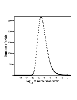
We have measured the numerical error by the value

$$\frac{\|\mathbf{K}-\hat{\mathbf{K}}\|}{\|\hat{\mathbf{K}}\|},$$

where $\hat{\mathbf{K}}$ is the ground truth calibration matrix, $\|\cdot\|$ is the Frobenius norm. The distribution of the numerical error is reported in Figure 1, where the total number of trials is $10^{6}$.

The running time information for our implementation of the algorithm is given in Table 2.

Step	Projective reconstr.	Metric reconstr.
$\mu s$	7.9	28.4/root

Table 2. Average running times for the algorithm steps on a system with Intel Core i5 2.3 GHz processor.

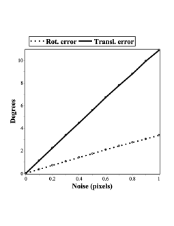
In Figure 2, we demonstrate the stability of the algorithm under increasing image noise. We have added a Gaussian noise with a standard deviation varying from 0 to 1 pixel in a $352\times 288$ image. Each point is a median of $10^{6}$ trials.

4.1. Outliers

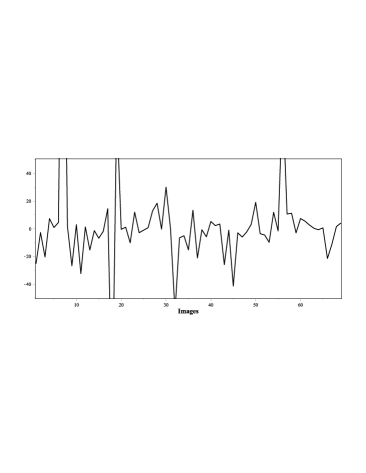
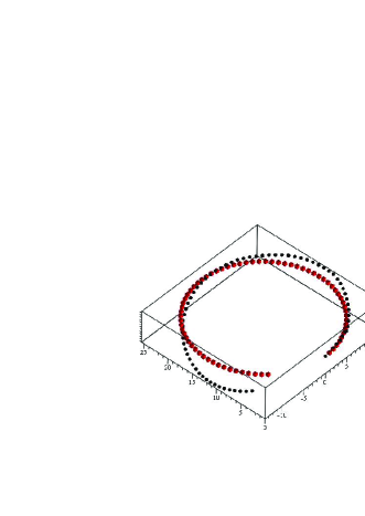
To test the algorithm in presence of outliers (incorrect matches), we have modeled a sequence of 70 cameras with centers on a circle, and 400 scene points viewed by all the cameras. For each image, we have added a Gaussian noise with one pixel standard deviation and $20\%$ of outliers (uniformly distributed points in the image plane).

The auto-calibration algorithm was used as a hypothesis generator within a random sample consensus (RANSAC) framework [2]. For better computational efficiency we used the preemptive RANSAC from [9]. The motion hypotheses were scored by the Sampson approximation to geometric error [5]. The number of hypotheses was set to 400 for each camera position, and the preemption block size was set to 100.

The results are presented in Figure 3 and Figure 4. No iterative refinements were performed in the estimation. The calibration matrix averaged from the image sequence is as follows:

$$\mathbf{K}=\begin{bmatrix}399.52&2.16&161.54\\ 0&405.37&142.14\\ 0&0&1\end{bmatrix}.$$

Figure 3. Skew parameter $K_{12}$ estimated from the sequence of 70 synthetic images. Average value of $K_{12}$ is $2.16$.

Figure 4. The camera track estimated from the sequence of 70 synthetic images. The red solid boxes are the ground truth camera positions.

5. Discussion

A new non-iterative auto-calibration algorithm is presented. It derives the camera calibration from the smallest possible number of views and scene points. A computation on synthetic data confirms its accuracy and high speed performance. The algorithm is quite flexible. It is reliable, for example, even in case of pure rotations (baseline $=0$), if the calibration matrix is only needed.

References

- [1] Faugeras, O. Three-Dimensional Computer Vision: A Geometric Viewpoint. MIT Press, 1993.
- [2] Fischler, M., Bolles, R. Random Sample Consensus: a Paradigm for Model Fitting with Application to Image Analysis and Automated Cartography. Commun. Assoc. Comp. Mach., Vol. 24, 381–395, 1981.
- [3] Hartley R. Estimation of Relative Camera Positions for Uncalibrated Cameras. Proceedings of the 2nd European Conference on Computer Vision, Vol. 588 of Lecture Notes in Computer Science, 579–587, 1992.
- [4] Hartley, R.I. Self-calibration from Multiple Views with a Rotating Camera. Proceedings of the 3rd European Conference on Computer Vision, Vol. 800–801 of Lecture Notes in Computer Science, 471–478, 1994.
- [5] Hartley, R., Zisserman, A. Multiple View Geometry in Computer Vision. Second Edition. Cambridge University Press, 2004.
- [6] Heikkilä, J. Geometric Camera Calibration Using Circular Control Points. IEEE Transactions on Pattern Analysis and Machine Intelligence, Vol. 22, No. 10, 1066–1077, 2000.
- [7] Maybank, S.J., Faugeras, O.D. A Theory of Self Calibration of a Moving Camera. International Journal of Computer Vision, Vol. 8, No. 2, 123- 151, 1992.
- [8] Mendonca, P.R.S., Cipolla, R. A Simple Technique for Self-Calibration. Proceedings of the IEEE International Conference on Computer Vision and Pattern Recognition, 500–505, 1999.
- [9] Nistér, D. Preemptive RANSAC for Live Structure and Motion Estimation. Proceedings of the Ninth IEEE International Conference on Computer Vision, 199–206, 2003.
- [10] Quan, L., Triggs, B. A Unification of Autocalibration Methods. Proceedings of the Fourth Asian Conference on Computer Vision, 917–922, 2000.
- [11] Schaffalitzky, F., Zisserman, A., Hartley, R.I., Torr, P.H.S. A Six Point Solution for Structure and Motion. Proceedings of the European Conference on Computer Vision, Vol. 1, 632–648, 2000.
- [12] Sturm, P. Critical Motion Sequences for Monocular Self-Calibration and Uncalibrated Euclidean Reconstruction. Proceedings of the International Conference on Computer Vision and Pattern Recognition, 1100–1105, 1997.
- [13] Triggs, B. Autocalibration and the Absolute Quadric. Proceedings of the IEEE International Conference on Computer Vision and Pattern Recognition, 609–614, 1997.
- [14] Tsai, R.Y. A Versatile Camera Calibration Technique for High-accuracy 3D Machine Vision Metrology Using Off-the-shelf TV Cameras and Lenses. J. Robotics and Automation, Vol. 3, No. 4, 323–344, 1987.
- [15] Zhang, Z. A Flexible New Technique for Camera Calibration. IEEE Transactions on Pattern Analysis and Machine Intelligence, Vol. 22, No. 11, 1330–1334, 2000.