MCMC Learning

Abstract

The theory of learning under the uniform distribution is rich and deep, with connections to cryptography, computational complexity, and the analysis of boolean functions to name a few areas. This theory however is very limited due to the fact that the uniform distribution and the corresponding Fourier basis are rarely encountered as a statistical model.

A family of distributions that vastly generalizes the uniform distribution on the Boolean cube is that of distributions represented by Markov Random Fields (MRF). Markov Random Fields are one of the main tools for modeling high dimensional data in many areas of statistics and machine learning.

In this paper we initiate the investigation of extending central ideas, methods and algorithms from the theory of learning under the uniform distribution to the setup of learning concepts given examples from MRF distributions. In particular, our results establish a novel connection between properties of MCMC sampling of MRFs and learning under the MRF distribution.

1 Introduction

The theory of learning under the uniform distribution is well developed and has rich and beautiful connections to discrete Fourier analysis, computational complexity, cryptography and combinatorics to name a few areas. However, these methods are very limited since they rely on the assumption that examples are drawn from the uniform distribution over the Boolean cube or other product distributions. In this paper we make a first step in extending ideas, techniques and algorithms from this theory to a much broader family of distributions, namely, to Markov Random Fields.

1.1 Learning Under the Uniform Distribution

Since the seminal work of Linial et al. (1993), the study of learning under the uniform distribution has developed into a major area of research; the principal tool is the simple and explicit Fourier expansion of functions defined on the boolean cube (${\{-1,1\}}^{n}$):

$$f(x)=\sum_{S\subseteq[n]}\hat{f}(S)\chi_{S}(x),\quad\chi_{S}(x)=\prod_{i\in S}x_{i}.$$

This connection allows a rich class of algorithms that are based on learning coefficients of $f$ for several classes of functions. Moreover, this connection allows application of sophisticated results in the theory of Boolean functions including hyper-contractivity, number theoretic properties and invariance, e.g.  (O’Donnell and Servedio, 2007, Shpilka and Tal, 2011, Klivans et al., 2002). On the other hand, the central role of the uniform distribution in computational complexity and cryptography relates learning under the uniform distribution to key themes in theoretical computer science including de-randomization, hardness and cryptography, e.g.  (Kharitonov, 1993, Naor and Reingold, 2004, Dachman-Soled et al., 2008).

Given the elegant theoretical work in this area, it is a little disappointing that these results and techniques impose such stringent assumptions on the underlying distribution. The assumption of independent examples sampled from the uniform distribution is an idealization that would rarely, if ever, be applicable in practice. In real distributions, features are correlated and correlations deem the analysis of algorithms that assume independence useless. Thus, it is worthwhile to ask the following question:
Question 1: Can the Fourier Learning Theory extend to correlated features?

1.2 Markov Random Fields

Markov random fields are a standard way of representing high dimensional distributions (see e.g.  (Kinderman and Snell, 1980)). Recall that a Markov random field on a finite graph $G=(V,E)$ and taking values in a discrete set ${\mathcal{A}}$, is a probability distribution on ${\mathcal{A}}^{V}$ of the form $\Pr[(\sigma_{v})_{v\in V}]=Z^{-1}\prod_{C}\phi_{C}((\sigma_{v})_{v\in C})$, where the product is over all cliques $C$ in the graph, $\phi_{C}$ are some non-negative valued functions and $Z$ is the normalization constant. Here $(\sigma_{v})_{v\in V}$ is an assignment from $V\rightarrow{\mathcal{A}}$.

Markov Random Fields are widely used in vision, computational biology, biostatistics, spatial statistics and several other areas. The popularity of Markov Random Fields as modeling tools is coupled with extensive algorithmic theory studying sampling from these models, estimating their parameters and recovering them. However, to the best of our knowledge the following question has not been studied.
Question 2: For an unknown function $f:{\mathcal{A}}^{V}\to\{-1,1\}$ from a class ${\mathcal{F}}$ and labeled samples from the Markov Random Field, can we learn the function?
Of course the problem stated above is a special case of learning a function class given a general distribution (Valiant, 1984, Kearns and Vazirani, 1994). Therefore, a learning algorithm that can be applied for a general distribution can be also applied to MRF distributions. However, the real question that we seek to ask above is the following: Can we utilize the structure of the MRF to obtain better learning algorithms?

1.3 Our Contributions

In this paper we begin to provide an answer to the questions posed above. We show how methods that have been used in the theory of learning under the uniform distribution can be also applied for learning from certain MRF distributions.

This may sound surprising as the theory of learning under the uniform distribution strongly relies on the explicit Fourier representation of functions. Given an MRF distribution, one can also imagine expanding a function in terms of a Fourier basis for the MRF, the eigenvectors of the transition matrix of the Gibbs Markov Chain associated with the MRF, which are orthogonal with respect to the MRF distribution. It seems however that this approach is naïve since:

1. Each eigenvector is of size $|{\mathcal{A}}|^{|V|}$; how does one store them?

2. How does one find these eigenvectors?

3. How does one find the expansion of a function in terms of these eigenvectors?

MCMC Learning: The main effort in this paper is to provide an answer to the questions above. For this we use Gibbs sampling, which is a Markov chain Monte Carlo (MCMC) algorithm that is used to sample from an MRF. We will use this MCMC method as the main engine in our learning algorithms. The Gibbs MC is reversible and therefore its eigenvectors are orthogonal with respect to the MRF distribution. Also, the sampling algorithm is straightforward to implement given access to the underlying graph and potential functions. There is a vast literature studying the convergence rates of this sampling algorithm; our results require that the Gibbs samplers are rapidly mixing.

In Section 4, we show how the eigenvectors of the transition matrix of the Gibbs MC can be computed implicitly. We focus on the eigenvectors corresponding to the higher eigenvalues. These eigenvectors correspond to the stable part of the spectrum, i.e. the part that is not very sensitive to small perturbation. Perhaps surprisingly, despite the exponential size of the matrix, we show that it is possible to adapt the power iteration method to this setting.

A function from ${\mathcal{A}}^{V}\rightarrow\mathbb{R}$ can be viewed as a $|{\mathcal{A}}|^{|V|}$ dimensional vector and thus applying powers of the transition matrix to it results in another function from ${\mathcal{A}}^{V}\rightarrow\mathbb{R}$. Observe that the powers of a transition matrix define distributions in time over the state space of the the Gibbs MC. Thus, the value of the function obtained by applying powers of a transition matrix can be approximated by sampling using the Gibbs Markov chain. Our main technical result (see Theorem 1) shows that any function approximated by “top” eigenvectors of the transition matrix of the Gibbs MC can be expressed a linear combination of powers of the the transition matrix applied to a suitable collection of “basis” functions, whenever certain technical conditions hold.

The reason for focusing on the part of the spectrum corresponding to stable eigenvectors is twofold. First, it is technically easier to access this part of the spectrum. Furthermore, we think of eigenvectors corresponding to small eigenvalues as unstable. Consider Gibbs sampling as the true temporal evolution of the system and let $\nu$ be an eigenvector corresponding to a small eigenvalue. Then calculating $\nu(x)$ provides very little information on $\nu(y)$ where $y$ is obtained from $x$ after a short evolution of the Gibbs sampler. The reasoning just applied is a generalization of the classical reasoning for concentrating on the low frequency part of the Fourier expansion in traditional signal processing.

Noise Sensitivity and Learning: In the case of the uniform distribution, the noise sensitivity (with parameter $\epsilon$) of a boolean function $f$, is defined as the probability that $f(x)\neq f(y)$, where $x$ is chosen uniformly at random and $y$ is obtained from $x$ by flipping each bit with probability $\epsilon$. Klivans et al. (2002) gave an elegant characterization of learning in terms of noise sensitivity. Using this characterization, they showed that intersections and thresholds of halfspaces can be elegantly learned with respect to the uniform distribution. In Section 4.3, we show that the notion of noise sensitivity and the results regarding functions with low noise sensitivity can be generalized to MRF distributions.

Learning Juntas: We also consider the so-called junta learning problem. A junta is a function that depends only on a small subset of the variables. Learning juntas from i.i.d. examples is a notoriously difficult problem, see (Blum, 1992, Mossel et al., 2004). However, if the learning algorithm has access to labeled examples that are received from a Gibbs sampler, these correlated examples can be useful for learning juntas. We show that under standard technical conditions on the Gibbs MC, juntas can be learned in polynomial time by a very simple algorithm. These results are presented in Section 5.

Relation to Structure Learning: In this paper, we assume that learning algorithms have the ability to sample from the Gibbs Markov Chain corresponding to the MRF. While such data would be hard to come by in practice, we remark that there is a vast literature regarding learning the structure and parameters of MRFs using unlabeled data and that it has recently been established that this can be done efficiently under very general conditions (Bresler, 2014). Once the structure of the underlying MRF is known, Gibbs sampling is an extremely efficient procedure. Thus, the methods proposed in this work could be used in conjunction with the techniques for MRF structure learning. The eigenvectors of the transition matrix could be viewed as features for learning, thus the methods proposed in this paper can be viewed as feature learning.

1.4 Related Work

The idea of considering Markov Chains or Random Walks in the context of learning is not new. However, none of the results and models considered before give non-trivial improvements or algorithms in the context of MRFs. Work of Aldous and Vazirani (1995) studies a Markov chain based model where the main interest was in characterizing the number of new nodes visited. Gamarnik (1999) observed that after the mixing time a chain can simulate i.i.d. samples from the stationary distribution and thus obtained learning results for general Markov chains. Bartlett et al. (1994) and Bshouty et al. (2005) considered random walks on the discrete cube and showed how to utilize the random walk model to learn functions that cannot be easily learned from i.i.d. examples from the uniform distribution on the discrete cube. In this same model, Jackson and Wimmer (2014) showed that agnostic learning parities and PAC-learning thresholds of parities (TOPs) could be performed in quasi-polynomial time.

2 Preliminaries

Let $X$ be an instance space. In this paper, we will assume that $X$ is finite and in particular we are mostly interested in the case when $X={\mathcal{A}}^{n}$, where ${\mathcal{A}}$ is some finite set. For $x,x^{\prime}\in{\mathcal{A}}^{n}$, let $d_{H}(x,x^{\prime})$ denote the Hamming distance between $x$ and $x^{\prime}$, i.e. $d_{H}(x,x^{\prime})=|\{i~{}|~{}x_{i}\neq x^{\prime}_{i}\}|$.

Let $M=\langle X,P\rangle$ denote a time-reversible discrete time ergodic Markov chain with transition matrix $P$. When $X={\mathcal{A}}^{n}$, we say that $M$ has single-site transitions if for any legal transition $x\rightarrow x^{\prime}$ it is the case that $d_{H}(x,x^{\prime})\leq 1$, i.e. $P(x,x^{\prime})=0$ when $d_{H}(x,x^{\prime})>1$. Let $X^{0}=x_{0}$ denote the starting state of a Markov chain $M$. Let $P^{t}(x_{0},\cdot)$ denote the distribution over states at time $t$, when starting from $x_{0}$. Let $\pi$ denote the stationary distribution of $M$. Denote by $\tau_{M}(x_{0})$ the quantity:

$$\tau_{M}(x_{0})=\min\{t:{\|P^{t}(x_{0},\cdot)-\pi\|_{\mbox{\footnotesize{TV}}}}\leq\frac{1}{4}\}$$

Then, define the mixing time of $M$ as $\tau_{M}=\max_{x_{0}\in X}\tau_{M}(x_{0})$. We say that a Markov chain with state space $X={\mathcal{A}}^{n}$ is rapidly mixing if $\tau_{M}\leq\mathrm{poly}(n)$.

While all the results in this paper are general, we describe two basic graphical models that will aid the discussion.

2.1 Ising Model

Consider a collection of nodes, $[n]=\{1,\ldots,n\}$, and for each pair $i,j$, there is an associated interaction energy, $\beta_{ij}$. Suppose $([n],E)$ denotes the graph, where $\beta_{ij}=0$ for $(i,j)\not\in E$. A state $\sigma$ of the system consists of an assignment of spins, $\sigma_{i}\in\{+1,-1\}$, to the nodes $[n]$. The Hamiltonian of configuration $\sigma$ is defined as

$$H(\sigma)=-\sum_{(i,j)\in E}\beta_{ij}\sigma_{i}\sigma_{j}-B\sum_{i\in[n]}\sigma_{i},$$

where $B$ is the external field. The energy of a configuration $\sigma$ is $\exp(-H(\sigma))$.

The Glauber dynamics on the Ising model defines the Gibbs Markov Chain $M=\langle{\{-1,1\}}^{n},P\rangle$, where the transitions are defined as follows:
  (i) In state $\sigma$, pick a node $i\in[n]$ uniformly at random. With probability $1/2$ do nothing, otherwise
  (ii) Let $\sigma^{\prime}$ be obtained by flipping the spin at node $i$. Then, with probability $\exp(-H(\sigma^{\prime}))/(\exp(-H(\sigma)+\exp(-H(\sigma^{\prime})))\}$, the state at the next time-step is $\sigma^{\prime}$. Otherwise the state at the next time-step remains unchanged.

The stationary distribution of the above dynamics is the Gibbs distribution, where $\pi(\sigma)\propto\exp(-H(\sigma))$. It is known that there exists a $\beta(\Delta)>0$ such that for all graphs of maximal degree $\Delta$, if $\max|\beta_{i,j}|<\beta(\Delta)$ then the dynamics above is rapidly mixing (Dobrushin and Shlosman, 1985, Mossel and Sly, 2013).

2.2 Graph Coloring

Let $G=([n],E)$ be a graph. For any $q>0$, a valid $q$-coloring of the graph $G$ is a function $C:V\rightarrow[q]$ such that for every $(i,j)\in E$, $C(i)\neq C(j)$. For a node $i$, let $N(i)=\{j~{}|~{}(i,j)\in E\}$ denote the set of neighbors of $i$. Consider the Markov chain defined by the following transition:
  (i) In state (valid coloring) $C$, choose a node $i\in[n]$ uniformly at random. With probability $1/2$ do nothing, otherwise:
  (ii) Let $S\subseteq[q]$ be the subset of colors defined by $S=\{C(j)~{}|~{}j\in N(i)\}$. Define $C^{\prime}$ to be the coloring obtained by choosing a random color $c\in[q]\setminus S$ and set $C^{\prime}(i)=c$, $C^{\prime}(j)=C(j)$ for $j\neq i$. The state at the next time-step is $C^{\prime}$.

The stationary distribution of the above Markov chain is uniform over the valid colorings of the graph. It is known that the above chain is rapidly mixing when the condition $q\geq 3\Delta$ is satisfied, where $\Delta$ is the maximal degree of the graph (in fact much better results are known (Jerrum, 1995, Vigoda, 1999)).

3 Learning Models

Let $X$ be a finite instance space and let $M=\langle X,P\rangle$ be an irreducible discrete-time reversible Markov chain, where $P$ is the transition matrix. Let $\pi_{M}$ denote the stationary distribution of $M$, $\tau_{M}$ the mixing time. We assume that the Markov chain $M$ is rapidly mixing, i.e. $\tau_{M}\leq\mathrm{poly}(\log(|X|))$ (note that if $X={\mathcal{A}}^{n}$, $\log(|X|)=O(n)$).

We consider the problem of learning with respect to stationary distributions of rapidly mixing Markov chains (e.g. defined by an MRF). The two graphical models described in the previous section serve as examples of such settings. The learning algorithm has access to the one-step oracle, $\mathsf{OS}(\cdot)$, that when queried with a state $x\in X$, returns the state after one step. Thus, $\mathsf{OS}(x)$ is a random variable with distribution $P(x,\cdot)$ and can be used to simulate the Markov chain.

Let ${\mathcal{F}}$ be a class of boolean functions over $X$. The goal of the learning algorithm is to learn an unknown function, $f\in{\mathcal{F}}$, with respect to the stationary distribution $\pi_{M}$ of the Markov chain $M$. As described above, the learning algorithm has the ability to simulate the Markov chain using the one-step oracle. We will consider both PAC learning and agnostic learning. Let $L:X\rightarrow\{-1,1\}$ be a (possibly randomized) labeling function. In the case of PAC learning $L$ is just the target function $f$; in the case of agnostic learning $L$ is allowed to be completely arbitrary. Let $D$ denote the distribution over $X\times{\{-1,1\}}$, where for any $(x,y)\sim D$, $x\sim\pi_{M}$ and $y=L(x)$.
PAC Learning (Valiant, 1984): In PAC learning the labeling function is the target function $f$. The goal of the learning algorithm is to output a hypothesis, $h:X\rightarrow{\{-1,1\}}$, which with probability at least $1-\delta$ satisfies $\operatorname{err}(h)=\Pr_{x\sim\pi_{M}}[h(x)\neq f(x)]\leq\epsilon$.
Agnostic Learning (Kearns et al., 1994, Haussler, 1992): In agnostic the labeling function $L$ may be completely arbitrary. Let $D$ be the distribution as defined above. Let $\mathrm{opt}=\min_{f\in{\mathcal{F}}}\Pr_{(x,y)\sim D}[f(x)\neq y]$. The goal of the learning algorithm is to output a hypothesis, $h:X\rightarrow{\{-1,1\}}$, which with probability at least $1-\delta$ satisfies,

$$\operatorname{err}(h)=\Pr_{(x,y)\sim D}[h(x)\neq y]\leq\mathrm{opt}+\epsilon$$

Typically, one requires that the learning algorithm have time and sample complexity that is polynomial in $n$, $1/\epsilon$ and $1/\delta$. So far, we have not mentioned what access the learning algorithm has to labeled examples. We consider two possible settings.

Learning with i.i.d. examples only: In this setting, in addition to having access to the one-step oracle, $\mathsf{OS}(\cdot)$, the learning algorithm has access to the standard example oracle, which when queried returns an example $(x,L(x))$, where $x\sim\pi_{M}$ and $L$ is the (possibly randomized) labeling function.

Learning with labeled examples from MC: In this setting, the learning algorithm has access to a labeled random walk, $(x^{1},L(x^{1})),(x^{2},L(x^{2})),\ldots,$ of the Markov chain. Here $x^{i+1}$ is the (random) state one time-step after $x^{i}$ and $L$ is the labeling function. Thus, the learning algorithm can potentially exploit correlations between consecutive examples.

The results in Section 4 only require access to i.i.d. examples. Note that these are sufficient to compute inner products with respect to the underlying distribution, a key requirement for Fourier analysis. The result in Section 5 is only applicable in the stronger setting where the learning algorithm receives examples from a labeled Markov chain. Note that since the chain is rapidly mixing, the learning algorithm by itself is able to (approximately) simulate i.i.d. random examples.

4 Harmonic Analysis using Eigenvectors

In this section, we show that the eigenvectors of the transition matrix can be (approximately) expressed as linear combinations of a suitable collection of basis functions and powers of the transition matrix applied to them.

Let $M=\langle X,P\rangle$ be a time-reversible discrete Markov chain. Let $\pi$ be the stationary distribution of $M$. We consider the set of right-eigenvectors of the matrix $P$. The largest eigenvalue of $P$ is $1$ and the corresponding eigenvector has $1$ in each co-ordinate. The left-eigenvector in this case is the stationary distribution. For simplicity of analysis we assume that $P(x,x)\geq 1/2$ for all $x$ which implies that all the eigenvalues of $P$ are non-negative. We are interested in identifying as many as possible of the remaining eigenvectors with eigenvalues less than $1$.

For functions, $f,g:X\rightarrow\mathbb{R}$, define the inner-product, $\langle f,g\rangle=\mathbb{E}_{x\sim\pi}[f(x)g(x)]$, and the norm $\|f\|_{2}=\sqrt{\langle f,f\rangle}$. Throughout this section, we will always consider inner products and norms with respect to the distribution $\pi$.

Since $M$ is reversible, the right eigenvectors of $P$ are orthogonal with respect to $\pi$. Thus, these eigenvectors can be used as a basis to represent functions from $X\rightarrow\mathbb{R}$. First, we briefly show that this approach generalizes the standard Fourier analysis on the Boolean cube, which is commonly used in uniform-distribution learning.

4.1 Fourier Analysis over the Boolean Cube

Let ${\{-1,1\}}^{n}$ denote the boolean cube. For $S\subseteq[n]$, the parity function over $S$ is defined as $\chi_{S}(x)=\prod_{i\in S}x_{i}$. With respect to the uniform distribution $U_{n}$ over ${\{-1,1\}}^{n}$, the set of parity functions $\{\chi_{S}~{}|~{}S\subseteq[n]\}$ form an orthonormal Fourier basis, i.e. for $S\neq T$, $\mathbb{E}_{x\sim U_{n}}[\chi_{S}(x)\chi_{T}(x)]=0$ and $\mathbb{E}_{x\sim U_{n}}[\chi_{S}(x)^{2}]=1$.

We can view the uniform distribution over ${\{-1,1\}}^{n}$ as arising from the stationary distribution of the following simple Markov chain. For $x,x^{\prime}$, such that $x_{i}\neq x_{i}^{\prime}$ and $x_{j}=x^{\prime}_{j}$ for $j\neq i$, let $P(x,x^{\prime})=1/(2n)$; $P(x,x)=1/2$. The remaining values of the matrix $P$ are set to $0$. This chain is rapidly mixing with mixing time $O(n\log(n))$ and the stationary distribution is the uniform distribution over ${\{-1,1\}}^{n}$. It is easy to see and well known that every parity function $\chi_{S}$ is an eigenvector of $P$ with eigenvalue $1-|S|/n$. Thus, Fourier-based learning under the uniform distribution can be seen as a special case of Harmonic analysis using eigenvectors of the transition matrix.

4.2 Representing Eigenvectors Implicitly

As in the case of the uniform distribution over the boolean cube, we would like to find the eigenvectors of the transition matrix of a general Markov chain, $M$, and use these as an orthonormal basis for learning. Unfortunately, in most cases of interest explicit succinct representations of eigenvectors don’t necessarily exist and the size of the set $|X|$ is likely to be prohibitively large, typically exponential in $n$, where $n$ is the length of the vectors in $X$. Thus, it is not possible to use standard techniques to obtain eigenvectors of $P$. Here, we show how these eigenvectors may be computed implicitly.

An eigenvector of the transition matrix $P$ is a function $\nu:X\rightarrow\mathbb{R}$. Throughout this section, we will view any function $g:X\rightarrow\mathbb{R}$ as an $|X|$-dimensional vector with value $g(x)$ at position $x$. As such, even writing down such a vector corresponding to an eigenvector $\nu$ is not possible in polynomial time. Instead, our goal is to show that whenever a suitable collection of basis functions exists, the eigenvectors have a simple representation in terms of these basis functions and powers of the transition matrix applied to them, as long as the underlying Markov chain $M$ satisfies certain conditions. The condition we require is that the spectrum of the transition matrix be discrete, i.e. eigenvalues show sharp drops. Between these drops, the eigenvalues may be quite close to each other, and in fact even equal. Figure 1 shows the spectrum of the transition matrix of the Ising model on a cycle of $10$ nodes for various values of $\beta$, the inverse temperature parameter. The case when $\beta=0$ corresponds to the uniform distribution on $\{-1,1\}^{10}$. One notices that the spectrum is discrete for small values of $\beta$ (high-temperature regime).

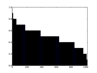
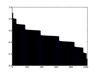
$\beta=0.00$	$\beta=0.02$
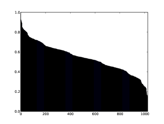
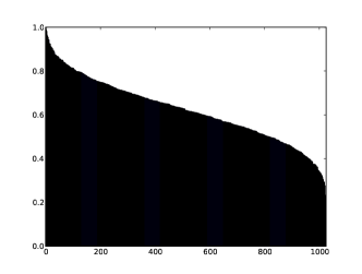
$\beta=0.1$	$\beta=1.00$

Figure 1: Spectrum of the transition matrix of the Gibbs MC for the Ising model on a cycle of length $10$ for various values of $\beta$, the inverse temperature parameter.

Next, we formally define the requirements of a discrete spectrum.

Definition 1 (Discrete Spectrum).

Let $P$ be the transition matrix of a Markov chain and let $\lambda_{1}\geq\lambda_{2}\geq\cdots\geq\lambda_{i}\geq\cdots\geq 0$ be the eigenvalues of $P$ in non-increasing order. We say that $P$ has an $(N,k,\gamma,c)$-discrete spectrum, if there exists a sequence $1\leq i_{1}\leq i_{2}\leq\cdots\leq i_{k}\leq|X|$ such that the following are true

1. Between $\lambda_{i_{j}}$ and $\lambda_{i_{j}+1}$, there is a non-trivial gap, i.e. for $j\in\{i_{1},\ldots,i_{k}\}$, $\frac{\lambda_{j+1}}{\lambda_{j}}\leq\gamma<1$

2. Let $i_{0}=1$, we refer to $S_{j}=\{i_{j-1}+1,\ldots,i_{j}\}$ as the $j{{}^{\textit{th}}}$ block (of eigenvalues and eigenvectors). Then the size of each block, $|S_{j}|\leq N$

3. The eigenvalue $\lambda_{i_{k}}$ is not too small (with respect to the gap at the end of each block), $\lambda_{i_{k}}\geq\gamma^{c}$

In general, the parameter $\gamma$ will depend on $n$ and we require that $\gamma\leq 1-1/\mathrm{poly}(n)$ in order to separate eigenvectors from the various blocks. One would expect $N$ to have dependence on both $n$ and $k$ and $c$ to have some dependence on $k$. As an example, we note that the spectrum corresponding to the Markov chain discussed in Section 4.1 is indeed discrete with the following parameters: $k$ can be any integer, $N=n^{k}$, $\gamma=1-(1/n)$ and $c=O(k)$.

In order to extract eigenvectors of $P$, we start with a collection of functions which have significant Fourier mass on the top eigenvectors. For an eigenvector $\nu$, it’s Fourier coefficient in any function $g:X\rightarrow\mathbb{R}$ is simply $\langle g,\nu\rangle$. Condition 2 in Definition 2 implicitly requires that the inner product $\langle g,\nu\rangle$ be large for $\nu$ with a large eigenvalue for some $g$ in the set. In addition, since eigenvalues corresponding to different eigenvectors may be equal or close together, we require a set of functions where the matrix corresponding to the Fourier coefficients of such eigenvectors is well-conditioned. Formally, we define the notion of a useful basis of functions with respect to a transition matrix $P$ which has an $(N,k,\gamma,c)$-discrete spectrum.

Definition 2 (Useful Basis).

Let ${\mathcal{G}}$ be a collection of functions from $X\rightarrow\mathbb{R}$. We say that ${\mathcal{G}}$ is $\alpha$-useful for an $(N,k,\gamma,c)$-discrete $P$ if the following hold:

1. For every $g\in{\mathcal{G}}$, $\|g\|_{\infty}\leq 1$

2. Let $i_{0}=0$, then for any $1\leq j\leq k$, if $N_{j}=i_{j}-i_{j-1}$ (the size of the $j{{}^{\textit{th}}}$ block), there exist $N_{j}$ functions $g_{1},\ldots,g_{N_{j}}\in{\mathcal{G}}$, such that the $N_{j}\times N_{j}$ matrix $A$ defined by $a_{m,l}=\langle g_{m},\nu_{l}\rangle$, where $m\in\{1,\ldots,N_{j}\}$ and $l\in\{i_{j-1}+1,\ldots,i_{j}\}$, has smallest singular value at least $1/\alpha$. Alternatively, the operator norm of $A^{-1}$, $\|A^{-1}\|_{op}$ is at most $\alpha$.

The parameter $\alpha$ will have dependence on $N$—a polynomial dependence on $N$ would result in efficient algorithms. In general, it is not known which Markov chains admit a useful basis that has a succinct representation. In the case of the uniform distribution, clearly the collection of parity functions already is such a useful basis. However, we observe that there are other useful bases as well. For example if for some $k$, one wished to extract all eigenvectors with eigenvalues at least $1-k/n$ (parities of size at most $k$), one can start with the collection of functions that is disjunctions (or conjunctions) on at most $k$ variables. Note that in this case, there is no contribution from eigenvectors with low eigenvalues (i.e. noise) in the basis functions. However, one would not expect to find such a useful basis without any contributions from eigenvectors with low eigenvalues when the stationary distribution is not product.

We now show how functions from a useful basis for a transition matrix with a discrete spectrum can be used to extract eigenvectors. First by applying powers of $P$ to some function $g$, the contributions of eigenvectors in different blocks can be separated. However, to separate eigenvectors within a block we require an incoherence condition among the various $g_{m}$s (which is the second condition in Definition 2). We first show that the eigenvectors $\nu$ can be approximately represented in the following form:

$$\nu\approx\sum_{t,m}\beta_{t,m}P^{t}g_{m},$$

where $m$ indexes the functions in ${\mathcal{G}}$.

Theorem 1.

Let $P$ be a transition matrix with an $(N,k,\gamma,c)$ discrete spectrum and let ${\mathcal{G}}$ be an $\alpha$-useful basis for $P$. Then for any $\epsilon>0$, there exists $\tau_{\mbox{\footnotesize{max}}}$ and $B$ such that every eigenvector $\nu_{\ell}$ with $\ell\leq i_{k}$ can be expressed as:

$$\nu_{\ell}=\sum_{t,m}\beta^{\ell}_{t,m}P^{t}g_{m}+\eta_{i}$$

where $\|\eta_{i}\|_{2}\leq\epsilon$, $t\leq\tau_{\mbox{\footnotesize{max}}}$ and $\sum_{t,m}|\beta_{t,m}|\leq B$. Furthermore,

$$B =(2\alpha Nk)^{\Theta((1+c)^{k+1})}\epsilon^{-(1+c)^{k}}$$

$$\tau_{max} =O\left(k(1+c)^{k-1}(\log(N)+\log(k)+\log(\alpha)++\frac{1}{\log(1/\gamma)}+\log(\frac{1}{\epsilon}))\right)$$

The proof of the above theorem is somewhat delicate and is provided in Appendix A.1. Notice that the bounds on $B$ and $\tau$ have a relatively mild (polynomial) dependence on most parameters except $k$ and $c$. Thus, when $c$ and $k$ are relatively small, for example both of them constant, both $B$ and $\tau$ are bounded by polynomials in the other parameters. Also, $N$ may be somewhat large, in the case of the uniform distribution $N=\Theta(n^{k})$—though this is still polynomial if $k$ is constant.

We can now use the above Theorem to devise a simple learning algorithm with respect to stationary distribution of the Markov chain. In fact, the learning algorithm does not even need to explicitly estimate the values of $\beta^{\ell}_{t,m}$ in the statement of Theorem 1—the result shows that any linear combination of the eigenvectors can also be represented as a linear combination of the collection of functions $\{P^{t}g_{m}\}_{t\leq\tau_{\mbox{\footnotesize{max}}},g_{m}\in{\mathcal{G}}}$. Thus, we can treat this collection as “features” and simply perform linear regression (either $L_{1}$ or $L_{2}$) as part of the learning algorithm. The algorithm is given in Figure 2. The key idea is to show that $P^{t}g_{m}(x)$ can be approximately computed for any $x\in X$ with blackbox access to $g_{m}$ and the one-step oracle $OS(\cdot)$. This is because $P^{t}g_{m}(x)=\mathbb{E}_{y\sim P^{t}(x,\cdot)}[g(y)]$, where $P^{t}(x,\cdot)$ is the distribution over $X$ obtained by starting from $x$ and taking $t$ steps of the Markov chain. The functions $\phi_{t,m}$ in the algorithm are computing approximations to $P^{t}g_{m}$ and then using them as features for learning. Formally, we can prove the following theorem.

Inputs: $\tau_{\mbox{\footnotesize{max}}},W,T$, blackbox access to $g\in{\mathcal{G}}$ and $\mathsf{OS}(\cdot)$, labeled examples $\langle(x_{i},y_{i})\rangle_{i=1}^{s}$ Preprocessing: For each $t\leq\tau_{\mbox{\footnotesize{max}}}$ and $m$ such that $g_{m}\in{\mathcal{G}}$ • For each $i=1,\ldots,s$, let $\displaystyle\phi_{t,m}(x_{i})=\frac{1}{T}\sum_{j=1}^{T}g_{m}(\mathsf{OS}^{t}_{j}(x_{i})),$ (1) where $\mathsf{OS}^{t}_{j}(x_{i})$ denotes the point obtained by an independent forward simulation of the Markov chain starting at $x_{i}$ for $t$ steps, for each $j$. Linear Program: Solve the following linear program: minimize $\displaystyle\sum_{i=1}^{s}\left|\sum_{t\leq\tau_{\mbox{\footnotesize{max}}},g_{m}\in{\mathcal{G}}}w_{t,m}\phi_{t,m}(x_{i})-y_{i}\right|$ subject to $\displaystyle\sum_{t\leq\tau_{\mbox{\footnotesize{max}}},g_{m}\in{\mathcal{G}}}|w_{t,m}|\leq W$ Output Hypothesis: • Let $h(x)=\displaystyle\sum_{t\leq\tau_{\mbox{\footnotesize{max}}},g_{m}\in{\mathcal{G}}}w_{t,m}\phi_{t,m}(x)$, where $\phi_{t,m}(x)$ are defined as in step (1) above. • Let $\theta\in[-1,1]$ be chosen uniformly at random and output $\operatorname{sign}(h(x)-\theta)$ as prediction

Figure 2: Agnostic Learning with respect to MRF distributions

Theorem 2.

Let $M=\langle X,P\rangle$ be a Markov chain and let $\lambda_{1}\geq\lambda_{2}\geq\cdots\geq 0$ denote the eigenvalues of $P$ and $\nu_{\ell}$ the eigenvector corresponding to $\lambda_{\ell}$. Let $\pi$ be the stationary distribution of $P$. Let ${\mathcal{F}}$ be a class of boolean functions. Suppose for some $\epsilon>0$, there exists $\ell^{*}(\epsilon)$ such that for every $f\in{\mathcal{F}}$,

$$\sum_{\ell>\ell^{*}}\langle f,\nu_{\ell}\rangle^{2}\leq\tfrac{\epsilon^{2}}{4},$$

i.e. every $f$ can be approximated (up to $\epsilon^{2}/4$) by the top $\ell^{*}$ eigenvectors of $P$. Suppose $P$ has a $(N,k,\gamma,c)$-discrete spectrum as defined in Definition 1, with $i_{k}\geq\ell^{*}$ and that ${\mathcal{G}}$ is an $\alpha$-useful basis for $P$. Then, there exists a learning algorithm that with blackbox access to functions $g\in{\mathcal{G}}$, the one-step oracle $\mathsf{OS}(\cdot)$ for Markov chain $M$, and access to random examples $(x,L(x))$ where $x\sim\pi$ and $L$ is an arbitrary labeling function, agnostically learns ${\mathcal{F}}$, up to error $\epsilon$.

Furthermore, the running time, sample complexity and the time required to evaluate the output hypothesis are bounded by a polynomial in $(Nk)^{(1+c)^{k+1}},\epsilon^{-(1+c)^{k}},|{\mathcal{G}}|,n$. In particular, if $\epsilon$ is a constant, $c$ and $k$ depend only on $\epsilon$ (and not on $n$), and $N\leq n^{\zeta(k)}$, where $\zeta$ may be an arbitrary function, the algorithm runs in polynomial time.

We give the proof this theorem in Appendix A.2; the proof uses the $L_{1}$-regression technique of Kalai et al. (2005). We comment that the learning algorithm (Fig. 2) is a generalization of the low-degree algorithm of Linial et al. (1993). Also, when applied to the Markov chain corresponding to the uniform distribution over ${\{-1,1\}}^{n}$, this algorithm works whenever the low-degree algorithm does (albeit with slightly worse bounds). As an example, we consider the algorithm of Klivans et al. (2002) to learn arbitrary functions of halfspaces. As a main ingredient of their work, they showed that halfspaces can be approximated by the first $O(1/\epsilon^{4})$ levels of the Fourier spectrum. The running time of our learning algorithm run with a useful basis consisting of parities, or conjunctions of size $O(1/\epsilon^{4})$ is polynomial (for constant $\epsilon$).

4.3 Noise Sensitivity Analysis

In light of Theorem 2, one can ask which function classes are well-approximated by top eigenvectors and for which MRFs. A generic answer is functions that are “noise-stable” with respect to the underlying Gibbs Markov chain. Below, we generalize the definition of noise sensitivity in the case of product distributions to apply under MRF distributions. In words, the noise sensitivity (with parameter $t$) of a boolean function $f$ is the probability that $f(x)$ and $f(y)$ are different, where $x\sim\pi$ is drawn from the stationary distribution and $y$ is obtained by taking $t$ steps of the Markov chain starting at $x$.

Definition 3.

Let $x\sim\pi$ from the stationary distribution of $P$ and $y\sim P^{t}(x,\cdot)$, the distribution obtained by taking $t$ steps of the Gibbs MC starting at $x$. For a boolean function $f:X\rightarrow\{-1,1\}$, define its noise sensitivity with respect to parameter $t$ and the transition matrix $P$ of the Gibbs MC as

$$\operatorname{NS}_{t}(f)=\Pr_{x\sim\pi,y\sim P^{t}(x,\cdot)}[f(x)\neq f(y)].$$

One can derive an alternative form for the noise sensitivity as follows. Let $\lambda_{1}\geq\lambda_{2}\geq\cdots 0$ denote the eigenvalues of $P$ and $\nu_{1},\nu_{2},\ldots$ the corresponding eigenvectors. Let $\hat{f}_{\ell}=\langle f,\nu_{\ell}\rangle$. Then,

$$\operatorname{NS}_{t}(f) =\Pr_{x\sim\pi,y\sim P^{t}(x,\cdot)}[f(x)\neq f(y)]$$

$$=\frac{1}{2}\mathbb{E}_{x\sim\pi,y\sim P^{t}(x,\cdot)}[1-f(x)f(y)]$$

$$=\frac{1}{2}-\frac{1}{2}\langle f,P^{t}f\rangle$$

$$=\frac{1}{2}-\frac{1}{2}\sum_{\ell}\lambda_{\ell}^{t}\hat{f}^{2}_{\ell}$$ (2)

The notion of noise-sensitivity has been fruitfully used in the theory of learning under the uniform distribution (see for example Klivans et al. (2002)). The main idea is that functions that have low noise sensitivity have most of their mass concentrated on “lower order Fourier coefficients”, i.e. eigenvectors with large eigenvalues. We show that this idea can be easily generalized in the context of MRF distributions. The proof of the following theorem is provided in Appendix A.3.

Theorem 3.

Let $P$ be the transition matrix of the Gibbs MC of an MRF and let $f:X\rightarrow\{-1,1\}$ be a boolean function. Let $\ell^{*}$ be the largest index such that $\lambda_{\ell^{*}}>\rho$, then:

$$\sum_{\ell>\ell^{*}}\hat{f}_{\ell}^{2}\leq\frac{e}{e-1}\operatorname{NS}_{-\frac{1}{\ln{\rho}}}(f)$$

Thus, it is of interest to study which function classes have low noise-sensitivity with respect to certain MRFs. As an example, we consider the Ising model on graphs with bounded degrees; the Gibbs MC in this case is the Glauber dynamics. We show that the class of halfspaces have low noise sensitivity with respect to this family of MRFs. In particular, the noise sensitivity with parameter $t$, only depends on $(t/n)$.

Proposition 1.

For every $\Delta\geq 0$, there exists $\beta(\Delta)>0$ such that the following holds: For every graph $G$ with maximum degree $\Delta$, the Ising model with $\beta<\beta(\Delta)$ and any function of the form $f=\operatorname{sign}(\sum_{i=1}^{n}w_{i}x_{i})$, it holds that $\operatorname{NS}_{t}(f)\leq\exp(-\delta(t/n))$, for some constant $\delta$ that depends only on $\Delta$.

The proof of the above proposition follows from Lemma 1 in Appendix A.4. As a corollary we get.

Corollary 1.

Let $P$ be the transition matrix of the Gibbs MC of an Ising model with bounded degree $\Delta$. Suppose that for some $\epsilon>0$, $P$ has an $(N,k,\gamma,c)$-discrete spectrum such that $k$ depends only on $\epsilon$ and $\Delta$, $\lambda_{i_{k}+1}<\exp(-\tfrac{\delta}{1}\cdot\tfrac{1}{\ln(4/\epsilon^{2})})$ (where $\delta$ is as in Proposition 1), $\gamma=1-1/\mathrm{poly}(n)$, $N$ is $\mathrm{poly}(n)$ and $c$ a constant, for constant $\epsilon,\Delta$. Furthermore, suppose that $P$ admits an $\alpha$-useful basis with $\alpha=\mathrm{poly}(n,1/\epsilon)$, for the parameters $(N,k,\gamma,c)$ as above. Then the class of halfspaces $\{\operatorname{sign}(\sum_{i}w_{i}x_{i})\}$, is agnostically learnable with respect to the stationary distribution $\pi$ of $P$ up to error $\epsilon$.

Proof.

Let $t=\tfrac{n}{\delta}\ln(4/\epsilon^{2})$, where $\delta$ is from Proposition 1. Thus, $\operatorname{NS}_{t}(f)\leq\epsilon^{2}/4$. Let $\rho=\exp(-1/t)$ (as in Theorem 3); by the assumption on $P$, $P$ admits an $(N,k,\gamma,c)$-distribution where $k$ depends only on $\epsilon,\Delta$, such that $\lambda_{i_{k}+1}<\rho$.

Now, the algorithm in Figure 2 together with the parameter settings from Theorems 1, 2 and 3 give the desired result. ∎

4.4 Discussion

In this section, we proposed that approximation using eigenvectors of the transition matrix of an appropriate Markov chain may be better than just polynomial approximation, when learning with respect to distributions defined by Markov random fields (not product). We checked this for a few different Ising models to approximate the majority function. Since the computations required are fairly intensive, we could only do this for relatively small models. However, we point that the methods proposed in this paper are highly-parallelizable and not beyond the reach of large computing systems. Thus, it may be of interest to run methods proposed here on larger datasets and real-world data.

Approximation of Majority: We look at three different graphs: a cycle of length 11, the complete graph on 11 nodes and an Erdős-Rényi random graph with $n=11$ and $p=0.3$. We looked at the Ising model on these graphs with various different values of $\beta$. In each case, we looked at degree-$k$ polynomial approximations for $k=2,4$ and also with using top $n^{k}$ eigenvectors of the majority function. We see that the approximation using eigenvectors is consistently better, except possibly for very low values of $\beta$, where polynomial approximations are also quite good. The values reported in the table are squared error for the approximation.

$\begin{array}[]{ccc}\mbox{ \begin{tabular}[]{|c|c|c|c|}\hline\cr$\beta$&Degree&Poly&Eigen\\ \hline\cr 0.02&2&0.3321&0.3550\\ &4&0.2084&0.1645\\ \hline\cr 0.05&2&0.3184&0.2322\\ &4&0.1937&0.1648\\ \hline\cr 0.1&2&0.2238&0.1417\\ &4&0.1199&0.0687\\ \hline\cr 0.2&2&0.1468&0.0018\\ &4&0.0034&0.0013\\ \hline\cr\end{tabular} }&\mbox{ \begin{tabular}[]{|c|c|c|c|}\hline\cr$\beta$&Degree&Poly&Eigen\\ \hline\cr 0.1&2&0.3330&0.3401\\ &4&0.2092&0.1606\\ \hline\cr 0.2&2&0.3307&0.2229\\ &4&0.2052&0.1538\\ \hline\cr 0.5&2&0.3113&0.1918\\ &4&0.1676&0.0715\\ \hline\cr 1.0&2&0.1857&0.0466\\ &4&0.0344&0.0253\\ \hline\cr\end{tabular} }&\mbox{ \begin{tabular}[]{|c|c|c|c|}\hline\cr$\beta$&Degree&Poly&Eigen\\ \hline\cr 0.05&2&0.3327&0.3404\\ &4&0.2089&0.2172\\ \hline\cr 0.1&2&0.3283&0.2240\\ &4&0.2034&0.1515\\ \hline\cr 0.2&2&0.3017&0.1897\\ &4&0.1757&0.1254\\ \hline\cr 0.5&2&0.0690&0.0326\\ &4&0.0262&0.0108\\ \hline\cr\end{tabular} }\\ \mbox{(a) $K_{11}$}&\mbox{(b) $C_{11}$}&\mbox{(c) $G(11,0.3)$}\end{array}$

Table 1: Approximation of the majority function using polynomials and eigenvectors for different Ising models

5 Learning Juntas

In this section, we consider the problem of learning the class of $k$-juntas. Suppose $X={\mathcal{A}}^{n}$ is the instance space. A $k$-junta is a boolean function that depends on only $k$ out of the $n$ possible co-ordinates of $x\in X$. In this section, we consider the model in which we receive labeled examples from a random walk of a Markov chain (see Section 3.2). In this case the learning algorithm can identify the $k$ relevant variables by keeping track of which variables caused the function to change its value.

For a subset, $S\subseteq[n]$ of the variables and a function $b_{S}:S\rightarrow{\mathcal{A}}$, let $x_{S}=b_{S}$ denote the event, $\bigwedge_{i\in S}x_{i}=b_{S}(x_{i})$, i.e. it fixes the assignment on the variables in $S$ as given by the function $b_{S}$. A set $S$ is the junta of function $f$, if the variables in $S$ completely determine the value of $f$. In this case, for $b_{S}:S\rightarrow{\mathcal{A}}$, every $x$ satisfying $x_{S}=b_{S}$ has the same value $f(x)$ and by slight abuse of notation we denote this common value by $f(b_{S})$.

Figure 3 describes the simple algorithm for learning juntas. Theorem 4 gives conditions under which Algorithm 3 is guaranteed to succeed. Later, we show that the Ising model and graph coloring satisfy these conditions.

Inputs: Access to labeled examples $(x,f(x))$ from Markov Chain $M$ Identifying Relevant Variables 1. ${\mathcal{J}}=\emptyset$ 2. Consider a random walk, $\langle(x^{1},f(x^{1})),\ldots,(x^{T},f(x^{T})\rangle$. 3. For every, $i$, such that $f(x^{i})\neq f(x^{i+1})$, if $j$ is the variable such that $x^{i}_{j}\neq x^{i+1}_{j}$, add $j$ to ${\mathcal{J}}$. Learning $f$ 1. Consider each of the $|{\mathcal{A}}|^{|{\mathcal{J}}|}$ possible assignments $b_{{\mathcal{J}}}\rightarrow{\mathcal{A}}$. We will construct a truth table for a function $h:{\mathcal{A}}^{{\mathcal{J}}}\rightarrow{\mathcal{Y}}$. 2. For a fixed $b_{{\mathcal{J}}}$, let $h(b_{{\mathcal{J}}})$ be the plurality label among the $x^{i}$ in the random walk above for which $x^{i}_{j}=b_{{\mathcal{J}}}(j)$ for all $j\in{\mathcal{J}}$. Output: Hypothesis $h$

Figure 3: Algorithm: Exact Learning $k$-juntas

Theorem 4.

Let $X={\mathcal{A}}^{n}$ and let $M=\langle X,P\rangle$ be a time-reversible rapidly mixing MC. Let $\pi$ denote the stationary distribution of $M$ and $\tau_{M}$ its mixing time. Furthermore, suppose that $M$ has single-site dynamics, i.e. $P(x,x^{\prime})=0$ if $d_{H}(x,x^{\prime})>1$ and that the following conditions hold:
   (i) For any $S\subseteq[n]$, $b_{S}:S\rightarrow{\mathcal{A}}$ either $\pi(x_{S}=b_{S})=0$ or $\pi(x_{S}=b_{S})\geq 1/(c|{\mathcal{A}}|)^{|S|}$, where $c$ is a constant.
   (ii) For any $x,x^{\prime}$ such that $\pi(x)\neq 0$, $\pi(x^{\prime})\neq 0$ and $d_{H}(x,x^{\prime})=1$, $P(x,x^{\prime})\geq\beta$.
Then Algorithm 3 exactly learns the class of $k$-junta functions with probability at least $1-\delta$ and the running time is polynomial in $n,|{\mathcal{A}}|^{k},\tau_{M},1/\beta,\log(1/\delta)$.

Proof.

Let $f$ be the unknown target $k$-junta function. Let $S$ be the set of variables that influence $f$, $|S|\leq k$. The set $S$ is called the junta for $f$. Note that a variable $i$ is in the junta for $f$, if and only if there exist $x,x^{\prime}\in{\mathcal{A}}^{n}$ such that $\pi(x)\neq 0$, $\pi(x^{\prime})\neq 0$, $x$, $x^{\prime}$ differ only at co-ordinate $i$ and $f(x)\neq f(x^{\prime})$. Otherwise, $i$ can have no influence in determining the value of $f$ (under the distribution $\pi$).

We claim that Algorithm 3 identifies every variable in the junta $S$ of $f$. Let $b_{S}:S\rightarrow{\mathcal{A}}$, be any assignment of values to variables in $S$. Since $S$ is the junta for $f$, any $x\in X$ that satisfies $x_{i}=b_{S}(i)$ for all $i\in S$, has the same value $f(x)$. By slight abuse of notation, we denote this common value by $f(b_{S})$.

The fact that $i\in S$ implies that there exist assignments, $b^{1}_{S}$, $b^{2}_{S}$, such that $b^{1}_{S}(i)\neq b^{2}_{S}(i)$, $\forall j\in S$, such that $j\neq i$, $b^{1}_{S}(j)=b^{2}_{S}(j)$ and which satisfy the following: $\pi(x_{S}=b^{1}_{S})\neq 0$, $\pi(x_{S},b^{2}_{S})\neq 0$. Consider the following event: $x$ is drawn from $\pi$, $x^{\prime}$ is the state after exactly one transition, $x$ satisfies the event $x_{S}=b^{1}_{S}$ and $x^{\prime}$ satisfies the event $x^{\prime}_{S}=b^{2}_{S}$. By our assumptions, the probability of this event is at least $\beta/(c|{\mathcal{A}}|)^{|S|}$. Let $\alpha=\beta/(c|{\mathcal{A}}|)^{|S|}$. Then, if we draw $x$ from the distribution $P^{t}(x_{0},\cdot)$ for $t=\tau_{M}\ln(2/\alpha)$, instead of the true stationary distribution $\pi$, the probability of the above event is still at least $\alpha/2$. This is because when $t=\tau_{M}\ln(2/\alpha)$, the ${\|P^{t}(x_{0},\cdot)-\pi\|_{\mbox{\footnotesize{TV}}}}\leq\alpha/2$. Thus, by observing a long enough random walk, i.e. one with $2\tau_{M}\ln(1/\alpha)\log(k/\delta)/\alpha$ transitions, except with probability $\delta/k$, the variable $i$ will be identified as a member of the junta. Since there are at most $k$ such variables, by a union bound all of $S$ will be identified. Once the set $S$ has been identified, the unknown function can be learned exactly by observing an example of each possible assignments to the variables in $S$. The above argument shows that all such assignments with non-zero measure under $\pi$ already exist in the observed random walk. ∎

Remark 1.

We observe that the condition that the MC be rapidly mixing alone is sufficient to identify at least one variable of the junta. However, unlike in the case of learning from i.i.d. examples, in this learning model, identifying one variable of the junta is not equivalent to learning the unknown junta function. In fact, it is quite easy to construct rapidly mixing Markov chains where the influence of some variables on the target function can be hidden, by making sure that the transitions that cause the function to change value happen only on a subset of the variables of the junta.

We now show that the Ising model and graph coloring satisfy the conditions of Theorem 4 as long as the underlying graphs have constant degree.

Ising Model: Recall that the state space is $X={\{-1,1\}}^{n}$. Let $\beta(\Delta)$ be the inverse critical temperature, which is a constant independent of $n$ as long as $\Delta$, the maximal degree, is constant. Let $S\subseteq[n]$ and let $b^{1}_{S}:S\rightarrow{\{-1,1\}}$ and $b^{2}_{S}:S\rightarrow{\{-1,1\}}$ be two distinct assignments to variables in $S$. Let $\sigma^{1},\sigma^{2}$ be two configurations of the Ising system such that for all $i\in S$, $\sigma^{1}_{i}=b^{1}_{S}(i)$, $\sigma^{2}_{i}=b^{2}_{S}(i)$ and for $i\not\in S$, $\sigma^{1}_{i}=\sigma^{2}_{i}$. Let $d^{1}=\sum_{(i,j)\in E:\sigma^{1}_{i}\neq\sigma^{1}_{j}}\beta_{ij}$ and $d^{2}=\sum_{(i,j)\in E:\sigma^{2}_{i}\neq\sigma^{2}_{j}}\beta_{ij}$. Then, since the maximum degree of the graph $\Delta$ is constant and each $\beta_{ij}$ is also bounded by some constant, $|d^{1}-d^{2}|\leq c|S|\Delta$. Then, by definition (see Section 2), $\exp(-c\beta\Delta|S|)\leq\pi(\sigma^{1})/\pi(\sigma^{2})\leq\exp(c\beta\Delta|S|)$. By summing over possible pairs $\sigma^{1},\sigma^{2}$ that satisfy the constraints, we have $\exp(-\beta\Delta|S|)\leq\pi(x_{S}=b^{1}_{S})/\pi(x_{S}=b^{2}_{S})\leq\exp(\beta\Delta|S|)$. But, since there are only $2^{|S|}$ possible assignments of variables in $S$, the first assumption of Theorem 4 follows immediately. The second assumption follows from the definition of the transition rate matrix, i.e. each non-zero entry in the transition rate matrix is at least $\exp(-\beta\Delta)/2n$.

Graph Coloring: Let $q$ be the number of colors. The state space is $[q]^{n}$ and invalid colorings have $0$ mass under the stationary distribution. We assume that $q\geq 3\Delta$, where $\Delta$ is the maximum degree in the graph. This is also the assumption that ensures rapid mixing. Let $S\subseteq[n]$ be an subset of nodes. Let $C^{1}_{S}$ and $C^{2}_{S}$ be two assignments of colors to the nodes in $S$. Let $D_{1}$ and $D_{2}$ be the set of valid colorings such that for each $x\in D_{1}$, $i\in S$, $x_{i}=C^{1}_{S}(i)$ and for each $x\in D_{2}$, $i\in S$, $x_{i}=C^{2}_{S}(i)$. We define a map from $D_{1}$ to $D_{2}$ as follows:

1. Starting from $x\in D_{1}$, first for all $i\in S$, set $x_{i}=C^{2}_{S}(i)$. This may in fact result in an invalid coloring.

2. The invalid coloring is switched to a valid coloring by only modifying neighbors of nodes in $S$. The condition that $q\geq 3\Delta$ ensures that this can always be done.

The above map has the following properties. Let $N(S)=\{j~{}|~{}(i,j)\in E,i\in S\}$. Then, the nodes that are not in $S\cup N(S)$ do not change the color. Thus, even though the map may be a many to one map, at most $q^{|S|+|N(S)|}$ elements in $D_{1}$ may be mapped to a single element in $D_{2}$. Note that $|S|+|N(S)|\leq(\Delta+1)|S|$. Thus, we have $\pi(D_{1})/\pi(D_{2})=|D_{1}|/|D_{2}|\leq q^{(\Delta+1)|S|}$. This implies the first condition of Theorem 4. The second condition follows from the definition of the transition matrix, each non-zero entry is at least $1/(2qn)$.

Appendix A Proofs from Section 4

A.1 Proof of Theorem 1

Proof.

We divide the spectrum of $P$ into blocks. Let $k$ and $i_{1},\ldots,i_{k}$ be as in Definition 1; furthermore define $i_{0}=0$ for notational convenience. For $j=1,\ldots,k$, let $S_{j}=\{i_{j-1}+1,\ldots,i_{j}\}$. Throughout this proof we use the letter $\ell$ to index eigenvectors of $P$—so $\nu_{\ell}$ is an eigenvector with eigenvalue $\lambda_{\ell}$. We want to find $\beta^{\ell}_{t,m}$ in order to (approximately) represent the eigenvector $\nu_{\ell}$ as

$$\nu_{\ell} =\sum_{t,m}\beta^{\ell}_{t,m}P^{t}g_{m}+\eta_{\ell}$$ (3)

Also, we use the notation,

$$\bar{\nu}_{\ell} =\sum_{t,m}\beta^{\ell}_{t,m}P^{t}g_{m},$$ (4)

We will show that such representations exist block by block. To begin define

$$\epsilon_{1} =\left(\frac{\epsilon}{(2\alpha N)^{\frac{1+c}{c}}(Nk)^{\frac{1}{2c}}}\right)^{(1+c)^{k-1}}$$ (5)

and define $$\epsilon_{j}$$ according to the following recurrence,

$$\epsilon_{j} =2\alpha N(Nk)^{\frac{1}{2(1+c)}}\epsilon_{j-1}^{\frac{1}{1+c}}$$ (6)

It is an easy calculation to verify that the solution for $$\epsilon_{j}$$ is given by

$$\epsilon_{j} =\left(2\alpha N(Nk)^{\frac{1}{2(1+c)}}\right)^{\frac{1+c}{c}\left(1-\frac{1}{(1+c)^{j-1}}\right)}\epsilon_{1}^{\frac{1}{(1+c)^{j-1}}}$$ (7)

Also, define

$$B_{1} =(N\alpha)^{c+1}\epsilon_{1}^{-c}$$ (8)

and let $$B_{j}$$ be defined according the following recurrence:

$$B_{j} =2\alpha N(Nk)^{\frac{1}{2(1+c)}}(\epsilon_{j-1})^{-\frac{c}{1+c}}B_{j-1}$$ (9)

It is an easy calculation to verify that the solution for $$B_{j}$$ is given by

$$B_{j} =\left(2N\alpha(Nk)^{\frac{1}{2(1+c)}}\right)^{j-1}\cdot\left(\prod_{j^{\prime}=1}^{j-1}\epsilon_{j^{\prime}}\right)^{-\frac{c}{1+c}}B_{1}$$ (10)

It can be verified that $\epsilon_{j}$ and $B_{j}$ are increasing as a function of $j$ as long as all $\epsilon_{j}$ remain smaller than $1$ (which can be verified by checking that $\epsilon_{k}<1$). We show by induction on $j$ that for any $\ell\in S_{j}$, $\sum_{t,m}|\beta^{\ell}_{t,m}|\leq B_{j}$ and $\|\eta_{\ell}\|_{2}\leq\epsilon_{j}$ (recall that the norm here is with respect to the distribution $\pi$).

Consider some $j$ and suppose that $|S_{j}|=N_{j}$. Denote by $S_{<j}=\displaystyle\bigcup_{j^{\prime}<j}S_{j^{\prime}}$, all the indices that precede those in $S_{j}$ and $S_{>j}=\{\ell^{\prime}~{}|~{}\ell^{\prime}>i_{j}\}$. According to Definition 2, there exist $g_{1},\ldots,g_{N_{j}}\in{\mathcal{G}}$, such that if $A$ is the $N_{j}\times N_{j}$ matrix given by $a_{m,\ell}=\langle g_{m},\nu_{\ell}\rangle$ for $\ell\in S_{j}$ and $1\leq m\leq N_{j}$, then $\|A^{-1}\|_{op}\leq\alpha$. Let $\bar{a}_{\ell,m}$ denote the element in position $(l,m)$ in $A^{-1}$ and let ${\mathcal{G}}_{j}=\{g_{1},\ldots,g_{N_{j}}\}$ be these specific $N_{j}$ functions in ${\mathcal{G}}$. Also, observe that by Definition 1, $N_{j}\leq N$.

Let $g_{m}\in{\mathcal{G}}_{j}$ and for any $\ell^{\prime}$, let $a_{m,\ell^{\prime}}=\langle g_{m},\nu_{\ell^{\prime}}\rangle$. Then, define

$$\tilde{g}_{m} =g_{m}-\sum_{\ell^{\prime}\in S_{<j}}a_{m,\ell^{\prime}}\bar{\nu}_{\ell^{\prime}}$$ (11)

Thus, $$\tilde{g}_{m} g_{m} j{{}^{\textit{th}}} \tilde{g}_{m}$$ is obtained from by (approximately) removing contributions of eigenvectors corresponding to blocks that precede the block. Thus, we may write as follows:

$$\tilde{g}_{m} =\sum_{\ell\in S_{j}}a_{m,\ell}\nu_{\ell}+\sum_{\ell^{\prime}\in S_{<j}}a_{m,\ell^{\prime}}(\nu_{\ell^{\prime}}-\bar{\nu}_{\ell^{\prime}})+\sum_{\ell^{\prime}\in S_{>j}}a_{m,\ell^{\prime}}\nu_{\ell^{\prime}}$$

$$=\sum_{\ell\in S_{j}}a_{m,\ell}\nu_{\ell}+\sum_{\ell^{\prime}\in S_{<j}}a_{m,\ell^{\prime}}\eta_{\ell^{\prime}}+\sum_{\ell^{\prime}\in S_{>j}}a_{m,\ell^{\prime}}\nu_{\ell^{\prime}}$$

To further simplify the above equation, define $$v^{<}_{m}=\sum_{l^{\prime}\in S_{<j}}a_{m,\ell^{\prime}}\eta_{\ell^{\prime}} v^{>}_{m}=\sum_{l^{\prime}\in S_{>j}}a_{m,\ell^{\prime}}\nu_{\ell^{\prime}}$$ and . Then, we have

$$\tilde{g}_{m} =\sum_{\ell\in S_{j}}a_{\ell,m}\nu_{\ell}+v^{<}_{m}+v^{>}_{m}$$ (12)

In the case of $v^{<}_{m}$, a crude bound can be established on its norm $\|v^{<}_{m}\|_{2}$ as follows: for any $\ell^{\prime}\in S_{<j}$, $\|\eta_{\ell^{\prime}}\|_{2}\leq\epsilon_{j-1}$ (induction hypothesis). Using the facts that $\sum_{\ell^{\prime}}(a_{m,\ell^{\prime}})^{2}\leq 1$, and that $|S_{<j}|\leq N(j-1)\leq Nk$, by applying the Cauchy-Schwarz inequality we get $\|v^{<}_{m}\|_{2}\leq\epsilon_{j-1}\sqrt{Nk}$.

For $v^{>}_{m}$, we note that $\|Pv^{>}_{m}\|_{2}\leq\lambda_{i_{j}+1}\|v^{>}_{m}\|_{2}$, since it only contains components corresponding to eigenvectors with eigenvalues at most $\lambda_{i_{j}+1}$. Also, note that $\|v^{>}_{m}\|_{2}^{2}\leq\sum_{\ell^{\prime}\in S_{>j}}(a_{m,\ell^{\prime}})^{2}\leq 1$.

We now complete the proof by induction. For, $j^{\prime}=1,\ldots,j-1$, suppose that all the eigenvectors corresponding to indices in $S_{j^{\prime}}$ have representations of the form in Equation (3) with parameters $B_{j^{\prime}}$ and $\epsilon_{j^{\prime}}$ respectively. Recall that $\bar{a}_{\ell,m}$ is the element in position $(\ell,m)$ of $A^{-1}$, where $A$ is the matrix defined as $a_{m,\ell}=\langle g_{m},\nu_{\ell}\rangle$ for $g_{m}\in{\mathcal{G}}_{j}$ and $\ell\in S_{j}$. Now for any $\ell\in S_{j}$, we can define $\bar{\nu}_{\ell}$ as follows (for the value $\tau_{j}$ to be specified later):

$$\bar{\nu}_{\ell} =\lambda_{\ell}^{-\tau_{j}}\sum_{m=1}^{N_{j}}\bar{a}_{\ell,m}P^{\tau_{j}}\tilde{g}_{m}$$ (13)

Using Equation (12) in the above equation, we get

$$\bar{\nu}_{\ell} =\lambda_{\ell}^{-\tau_{j}}\sum_{m=1}^{N_{j}}\bar{a}_{\ell,m}\sum_{\ell^{\prime}\in S_{j}}a_{m,\ell^{\prime}}P^{\tau_{j}}\nu_{\ell^{\prime}}+\lambda_{\ell}^{-\tau_{j}}\sum_{m=1}^{N_{j}}P^{\tau_{j}}v^{<}_{m}+\lambda_{\ell}^{-\tau}\sum_{m=1}^{N_{j}}\bar{a}_{\ell,m}P^{\tau_{j}}v^{>}_{m}$$

$$=\lambda_{\ell}^{-\tau_{j}}\sum_{\ell^{\prime}\in S_{j}}\lambda_{\ell^{\prime}}^{\tau_{j}}\nu_{\ell^{\prime}}\sum_{m=1}^{N_{j}}\bar{a}_{\ell,m}a_{m,\ell^{\prime}}+\lambda_{\ell}^{-\tau_{j}}\sum_{m=1}^{N_{j}}\bar{a}_{\ell,m}P^{\tau_{j}}v^{<}_{m}+\lambda_{\ell}^{-\tau_{j}}\sum_{m=1}^{N_{j}}\bar{a}_{\ell,m}P^{\tau_{j}}v^{>}_{m}$$

In the first term, we use the fact that $$\sum_{m}\bar{a}_{\ell,m}a_{m,\ell^{\prime}}=\delta_{\ell,\ell^{\prime}} \nu_{\ell}$$ by definition. Thus, the first term reduces to . We apply the triangle inequality to get

$$\|\eta_{\ell}\|_{2}=\|\nu_{\ell}-\bar{\nu}_{\ell}\|_{2} \leq\lambda_{\ell}^{-\tau_{j}}\left\|\sum_{m=1}^{N_{j}}\bar{a}_{\ell,m}P^{\tau_{j}}v^{<}_{m}\right\|_{2}+\lambda_{\ell}^{-\tau_{j}}\left\|\sum_{m=1}^{N_{j}}\bar{a}_{\ell,m}P^{\tau_{j}}v^{>}_{m}\right\|_{2}$$

$$\leq\lambda_{\ell}^{-\tau_{j}}\sqrt{\sum_{m=1}^{N_{j}}(\bar{a}_{\ell,m})^{2}}\cdot\sqrt{\sum_{m=1}^{N_{j}}\|P^{\tau_{j}}v^{<}_{m}\|_{2}^{2}}+\lambda^{-\tau_{j}}\sqrt{\sum_{m=1}^{N_{j}}(\bar{a}_{\ell,m})^{2}}\cdot\sqrt{\sum_{m=1}^{N_{j}}\|P^{\tau_{j}}v^{>}_{m}\|_{2}^{2}}$$ (14)

We use the fact that $$\sqrt{\sum_{i=1}^{m}(\bar{a}_{\ell,m})^{2}}\leq\|A^{-1}\|_{F} N_{j}\leq N \|v^{<}_{m}\|_{2}^{2}\leq Nk(\epsilon_{j-1})^{2} P 1 \|P^{\tau_{j}}v\|_{2}\leq\|v\|_{2} v v^{>}_{m} \|v^{>}_{m}\|_{2}\leq 1 \lambda_{i_{j}+1} \|P^{\tau_{j}}v^{<}_{m}\|_{2}\leq\lambda_{i_{j}+1}^{\tau_{j}}$$ and that , to simplify the above expression. Furthermore, since has largest eigenvalue , for any . In the case of , since the and the largest eigenvalue in it is , . Putting all these together and simplifying the above expression we get

$$\|\eta_{\ell}\|_{2} \leq\|A^{-1}\|_{F}\sqrt{N}\left(\lambda_{\ell}^{-\tau_{j}}\epsilon_{j-1}\sqrt{Nk}+\left(\frac{\lambda_{i_{j}+1}}{\lambda_{\ell}}\right)^{\tau_{j}}\right)$$

Finally, using the fact that $$\lambda_{\ell}\geq\lambda_{i_{j}} \ell\in S_{j} \lambda_{i_{j}+1}/\lambda_{\ell}\leq\gamma 1/\lambda_{\ell}\leq\gamma^{-c} \|A^{-1}\|_{F}\leq\sqrt{N}\|A^{-1}\|_{op}\leq\sqrt{N}\alpha$$ (since ), we have that and that . We also use the fact that . Thus, we get

$$\|\eta_{\ell}\|_{2} \leq\alpha N\left(\gamma^{-c\tau_{j}}\epsilon_{j-1}\sqrt{Nk}+\gamma^{\tau_{j}}\right)$$ (15)

At this point we will deal with the base case $j=1$ separately. In Equation (12) when $g_{m}\in{\mathcal{G}}_{1}$, $v^{<}_{m}=0$, since the set $S_{<1}$ is empty. Thus, in Equation (14), the first term is absent if we are dealing with the case when $\ell\in S_{1}$, since all the $v^{<}_{m}$ in this case are $0$. Thus, for $\ell\in S_{1}$, Equation (15) reduces to:

$$\|\eta_{\ell}\|_{2} \leq\alpha N\gamma^{\tau_{1}}$$ (16)

Thus, by choosing $\tau_{1}=-\frac{\ln(N\alpha/\epsilon_{1})}{\ln(\gamma)}$, we get that for all $\ell\in S_{1}$, $\|\eta_{\ell}\|_{2}\leq\epsilon_{1}$. Now, for $j>1$, we can find $\tau_{j}$ that minimizes the RHS of Equation (15) and this is given by $\tau_{j}=\frac{1}{1+c}\frac{\ln(\epsilon_{j-1}\sqrt{Nk})}{\ln(\gamma)}$. It is not hard to calculate that in this case the RHS of Equation 15 exactly evaluates to $\epsilon_{j}$.

We now prove a bound on $B_{j}$. Again, we look at the base case separately, when $j=1$, $S_{<j}=\emptyset$ and so for the functions $g_{m}\in{\mathcal{G}}_{1}$ as in Equation (11), $\tilde{g}_{m}=g_{m}$. Thus, for $\ell\in S_{1}$, by looking at Equation (13), we can define: $\beta^{\ell}_{\tau_{1},m}=\lambda_{\ell}^{-\tau_{1}}\bar{a}_{\ell,m}$ for $m\in{\mathcal{G}}_{1}$ and the remaining $\beta^{\ell}_{t,m}$ values are set to $0$. Thus,

$$\sum_{t,m}|\beta^{\ell}_{t,m}| \leq\lambda_{\ell}^{-\tau_{1}}\sum_{m=1}^{N_{1}}|\bar{a}_{\ell,m}|\leq\gamma^{-c\tau_{1}}N\alpha$$ (17)

Above we used the fact that $\lambda_{\ell}\geq\lambda_{i_{k}}\geq\gamma^{c}$ and that $|\bar{a}_{\ell,m}|\leq\|A^{-1}\|_{op}$. But, the RHS above is exactly the quantity $B_{1}$ we defined earlier.

Next, we consider the case of $j>1$ and we start from Equation (13).

$$\bar{\nu}_{\ell} =\lambda_{\ell}^{-\tau_{j}}\sum_{m=1}^{N_{j}}\bar{a}_{\ell,m}P^{\tau_{j}}\tilde{g}_{m}$$

$$=\lambda_{\ell}^{-\tau_{j}}\sum_{m=1}^{N_{j}}\bar{a}_{\ell,m}P^{\tau_{j}}\left(g_{m}-\sum_{\ell^{\prime}\in S_{<j}}a_{m,\ell^{\prime}}\bar{\nu}_{\ell^{\prime}}\right)$$

$$=\lambda_{\ell}^{-\tau_{j}}\sum_{m=1}^{N_{j}}\bar{a}_{\ell,m}P^{\tau_{j}}\left(g_{m}-\sum_{\ell^{\prime}\in S_{<j}}a_{m,\ell^{\prime}}\sum_{t,m^{\prime}}\beta^{\ell^{\prime}}_{t,m^{\prime}}P^{t}g_{m^{\prime}}\right)$$

$$=\lambda_{\ell}^{-\tau_{j}}\sum_{m=1}^{N_{j}}\bar{a}_{\ell,m}\left(P^{\tau_{j}}g_{m}-\sum_{\ell^{\prime}\in S_{<j}}a_{m,\ell^{\prime}}\sum_{t,m^{\prime}}\beta^{\ell^{\prime}}_{t,m^{\prime}}P^{t+\tau_{j}}g_{m^{\prime}}\right)$$ (18)

If the above, expression is re-written to be of the form,

$$\bar{\nu}_{\ell}=\sum_{t,m}\beta^{\ell}_{t,m}P^{t}g_{m},$$

we can get a bound on $$\sum_{t,m}|\beta^{\ell}_{t,m}|$$ as follows:

$$\sum_{t,m}|\beta^{\ell}_{t,m}| \leq\gamma^{-c\tau_{j}}\left(\sum_{m=1}^{N_{j}}|\bar{a}_{\ell,m}|\right)\cdot\left(1+B_{j-1}\sum_{\ell^{\prime}\in S_{<j}}|a_{m,\ell^{\prime}}|\right)$$

Above, we use the fact that for $$\ell^{\prime}\in S_{<j} \sum_{t,m}|\beta^{\ell^{\prime}}_{t,m}|\leq B_{j-1} \sum_{m=1}^{N_{j}}|\bar{a}_{\ell,m}|\leq N\alpha \sum_{\ell^{\prime}\in S_{<j}}|a_{m,\ell^{\prime}}|\leq\sqrt{Nk} \sum_{\ell^{\prime}}(a_{m,\ell^{\prime}})^{2}\leq 1 m$$, . Also, note that and (since for all ), so we have

$$\sum_{t,m}|\beta^{\ell}_{t,m}| \leq(\epsilon_{j-1}\sqrt{Nk})^{-\frac{c}{1+c}}N\alpha(1+\sqrt{Nk}B_{j-1})$$

$$\leq 2\sqrt{Nk}N\alpha B_{j-1}(\epsilon_{j-1}\sqrt{Nk})^{-\frac{c}{1+c}}$$

We observe that the expression on the RHS above is exactly the value $B_{j}$ given by the recurrence relation in Equation (9).

Finally, by observing the RHS of Equation (13) we notice that the maximum power $t$, for which $\beta^{\ell}_{t,m}$ is non-zero for any $\ell,m$ is $\sum_{i=1}^{k}\tau_{i}$. Thus, the proof is complete by setting $\tau_{\max}=\sum_{j=1}^{k}\tau_{j}$.

∎

A.2 Proof of Theorem 2

Proof.

Let $f\in F$ be the target function and for any $\ell$, let $\hat{f}_{\ell}=\langle f,\nu_{\ell}\rangle$ denote the Fourier coefficients of $f$. Then the condition in Theorem 2 states that $\sum_{\ell>\ell^{*}(\epsilon)}\hat{f}_{\ell}^{2}\leq\epsilon^{2}/4$.

First, we appeal to Theorem 1. In the rest of this proof, we assume that for all $\ell\leq\ell^{*}$, there exist $\beta^{\ell}_{t,m}$ such that

$$\nu_{\ell}=\sum_{t,m}\beta^{\ell}_{t,m}P^{t}g_{m}+\eta_{\ell},$$

where $g_{m}\in{\mathcal{G}}$, $\|\eta_{\ell}\|_{2}\leq\epsilon_{1}$. Furthermore, let $B$ and $\tau_{\mbox{\footnotesize{max}}}$ be as given by the statement of the theorem.

We first look closely at $P^{t}g_{m}$, since $P$ is an $|X|\times|X|$ matrix and $g_{m}:X\rightarrow\mathbb{R}$ a function, $P^{t}g_{m}$ is also a function from $X\rightarrow\mathbb{R}$. For $x\in X$, let $\mathds{1}_{x}$ denote the indicator function of the point $x$ (it may be viewed as a vector that is $0$ everywhere, except in position $x$ where it has value $1$). Then, we have

$$(P^{t}g_{m})(x) =\mathds{1}_{x}^{T}P^{t}g_{m}=\mathbb{E}_{y\sim P^{t}(x,\cdot)}[g_{m}(y)]$$ (19)

Notice that the quantity on the RHS above can be estimated by sampling. Thus, with black-box access to the oracle $\mathsf{OS}(\cdot)$ and $g_{m}$, we can estimate $(P^{t}g_{m})(x)$. This is exactly what is done in (1) in the algorithm in Figure 2. Also, since $\|g\|_{\infty}\leq 1$, it is also the case that $\|P^{t}g_{m}\|_{\infty}\leq 1$. Thus, by a standard Chernoff-Hoeffding bound, if we set the input parameter $T=\log(\tau_{\mbox{\footnotesize{max}}}\cdot|X|\cdot|{\mathcal{G}}|/\delta)/\epsilon_{2}^{2}$, with probability at least $1-\delta$, it holds for every $x\in X$, for every $t<\tau_{\mbox{\footnotesize{max}}}$ and every $g_{m}\in{\mathcal{G}}$, that $|\phi_{t,m}(x)-(P^{t}g_{m})(x)|\leq\epsilon_{2}$. For the rest of this proof, we will treat the functions $\phi_{t,m}(x)$ as deterministic (rather than randomized) for simplicity. (This can be easily arranged by taking a sufficiently long random string used to simulate the Markov chain and treating it as advice.)

Now, consider the following:

$$\mathbb{E}\left[\left(f(x)-\sum_{\ell\leq\ell^{*}}\hat{f}_{\ell}\sum_{t,m}\beta^{\ell}_{t,m}\phi_{t,m}(x)\right)^{2}\right]$$

$$~{}~{}~{}~{}~{}~{}\leq 2\mathbb{E}\left[\left(f(x)-\sum_{\ell\leq\ell^{*}}\hat{f}_{\ell}\nu_{\ell}(x)\right)^{2}\right]+2\mathbb{E}\left[\left(\sum_{\ell}\hat{f}_{\ell}\left(\nu_{\ell}(x)-\sum_{t,m}\beta^{\ell}_{t,m}\phi_{t,m}(x)\right)\right)^{2}\right]$$ (20)

Note that the first term above is at most $$\epsilon \bar{\nu}_{\ell}$$. We will now bound the second term. (Below is as defined in Equation (13).)

$$\mathbb{E}\left[\left(\sum_{\ell}\hat{f}_{\ell}\left(\nu_{\ell}(x)-\sum_{t,m}\beta^{\ell}_{t,m}\phi_{t,m}(x)\right)\right)^{2}\right]$$

$$~{}~{}~{}~{}~{}~{}\leq 2\mathbb{E}\left[\left(\sum_{\ell\leq\ell^{*}}\hat{f}_{\ell}(\nu(x)-\bar{\nu}(x))\right)^{2}\right]+2\mathbb{E}\left[\left(\sum_{\ell}\hat{f}_{\ell}\left(\sum_{t,m}\beta^{\ell}_{t,m}((P^{t}g_{m})(x)-\phi_{t,m}(x))\right)\right)^{2}\right]$$

$$~{}~{}~{}~{}~{}~{}\leq 2\sqrt{\sum_{\ell\leq\ell^{*}}(\hat{f}_{\ell})^{2}}\cdot\sqrt{\sum_{\ell\leq\ell^{*}}\|\eta_{\ell}\|_{2}^{2}}+2\sqrt{\sum_{\ell\leq\ell^{*}}(\hat{f}_{\ell})^{2}}\cdot\sqrt{\sum_{\ell<\ell^{*}}\left\|\sum_{t,m}\beta^{\ell}_{t,m}(P^{t}g_{m}-\phi_{t,m})\right\|^{2}_{2}}$$

Next we use the following facts, $$\sum_{\ell\leq\ell^{*}}(\hat{f}_{\ell})^{2}\leq 1 \ell^{*}\leq Nk \|\eta_{\ell}\|_{2}\leq\epsilon_{1} \sum_{t,m}|\beta^{\ell}_{t,m}|\leq B \forall x,|(P^{t}g_{m})(x)-\phi_{t,m}(x)|\leq\epsilon_{2} \|\sum_{t,m}\beta^{\ell}_{t,m}(P^{t}g_{m}-\phi_{t,m})\|_{2}\leq B\epsilon_{2}$$, and . Also for the very last term, the fact that and , imply that . Putting everything together we get

$$\mathbb{E}\left[\left(\sum_{\ell}\hat{f}_{\ell}\left(\nu_{\ell}(x)-\sum_{t,m}\beta^{\ell}_{t,m}\phi_{t,m}(x)\right)\right)^{2}\right]\leq 2(\sqrt{Nk\epsilon_{1}}+\sqrt{BNk\epsilon_{2}})$$ (21)

Finally, substituting (21) back into (20), we get

$$\mathbb{E}\left[\left(f(x)-\sum_{\ell\leq\ell^{*}}\hat{f}_{\ell}\sum_{t,m}\beta^{\ell}_{t,m}\phi_{t,m}(x)\right)^{2}\right]\leq 2(\frac{\epsilon^{2}}{4}+\sqrt{Nk\epsilon_{1}}+\sqrt{BNk\epsilon_{2}})$$ (22)

By choosing $$\epsilon_{1}=\epsilon^{2}/(64Nk) \epsilon_{2}=\epsilon^{2}/(64BNk) \epsilon^{2}$$ and we get that the quantity is in fact at most . Thus, we get that

$$\mathbb{E}\left[\left|f(x)-\sum_{\ell\leq\ell^{*}}\hat{f}_{\ell}\sum_{t,m}\beta^{\ell}_{t,m}\phi_{t,m}(x)\right|\right]=\epsilon$$ (23)

Thus, we have essentially shown that $\{\phi_{t,m}\}$ can be used as a suitable feature space and there is a linear form in this feature space that is a good $L_{1}$ approximation to $f$. This is sufficient for agnostic learning as was shown by Kalai et al. (2005). Note that the sum of coefficients on the features is bounded by $B\sqrt{Nk}$ (since $B$ is a bound on $\sum_{t,m}|\beta^{\ell}_{t,m}|$ and $\sum_{\ell<\ell^{*}}|\hat{f}_{\ell}|\leq\sqrt{Nk}$). Thus, in the algorithm in Figure 2, we may set the parameters $\tau_{\mbox{\footnotesize{max}}}$ (as given by Theorem 1), $W=B\sqrt{Nk}$ and $T=\log(\tau_{\mbox{\footnotesize{max}}}\cdot|X|\cdot|{\mathcal{G}}|/\delta)/\epsilon_{2}^{2}$. The sample complexity is polynomial in $W$, $1/\epsilon$ as follows from standard generalization bounds (see for example Kakade et al. (2008)) and the running time of the algorithm is polynomial in $|{\mathcal{G}}|,T,\tau_{\max},W,\frac{1}{\epsilon}$. The bounds given in the statement of the theorem follow from observing the values of the above quantity in the statement of Theorem 1. ∎

A.3 Proof of Theorem 3

Proof.

The proof follows the standard proofs of these types of results. Let $t=-\frac{1}{\ln(\rho)}$

$$\operatorname{NS}_{t}(f) =\frac{1}{2}-\frac{1}{2}\langle f,P^{t}f\rangle$$

$$=\frac{1}{2}-\frac{1}{2}\left(\sum_{\ell}\lambda_{\ell}^{t}\hat{f}^{2}_{\ell}\right)$$

$$\geq\frac{1}{2}-\frac{1}{2}\left(\sum_{\ell\leq\ell^{*}}\hat{f}^{2}_{\ell}+\sum_{\ell>\ell^{*}}\rho^{t}\hat{f}^{2}_{\ell}\right)$$

Using the fact that $$\sum_{\ell\leq\ell^{*}}\hat{f}^{2}_{\ell}=1-\sum_{\ell>\ell^{*}}\hat{f}^{2}_{\ell} f$$ (since is boolean) and rearranging terms, we get

$$\sum_{\ell>\ell^{*}}\hat{f}^{2}_{\ell} \leq\frac{1}{1-\rho^{t}}\operatorname{NS}_{t}(f)$$ (24)

Then substituting the value for $t$ completes the proofs. ∎

A.4 Proof of Proposition 1

Lemma 1.

For any positive integer $\Delta$, there exists $\beta(\Delta)$, such that for all graphs $G$ of maximum degree bounded by $\Delta$, and for all ferromagnetic Ising models with $\beta<\beta(\Delta)$, the following holds. If $f=\operatorname{sign}(\sum_{i}w_{i}x_{i})$, then for all $t\geq n$ it holds that,

$$1-2\operatorname{NS}_{t}(f)\geq\delta^{t/n}$$

for some fixed $\delta>0$ depending only on $\Delta$ and $\beta(\Delta)$.

Note that the above lemma only proves that majorities are somewhat noise stable. While one expects that if $t$ is a very small fraction on $n$, majorities are very noise stable, our proof is not strong enough to prove that.

For the proof we will need to use the following well known result which goes back to Dobrushin and Shlosman (1985). The proof also follows easily from the random cluster representation of the Ising model.

Lemma 2.

For every $\Delta$ and $\eta>0$, there exists a $\beta(\Delta,\eta)>0$ such that for all graphs $G$ of maximum degree bounded by $\Delta$ and for all Ising models where $\beta\leq\beta(\Delta,\eta)$, it holds that under the stationary measure for any $i$ and any subset $S$ of nodes,

$$\mathbb{E}[x_{i}~{}|~{}x_{S}]\leq\eta^{d(i,S)}$$

In particular, for every $i$ and $j$,

$$\mathbb{E}[x_{i}x_{j}]\leq\eta^{d(i,j)},$$

where $d(i,j)$ denotes the graph distance between $i$ and $j$.

We will need a few corollaries of the above lemma.

Lemma 3.

If $\beta<\beta(\Delta,1/(10\Delta))$, then for every set $A$ and any weights $w_{i}$, it holds that if $f(x)=\sum_{i}w_{i}x_{i}$, then:

1. $\frac{4}{5}\sum_{i}w_{i}^{2}\leq\mathbb{E}[f(x)^{2}]\leq\frac{6}{5}\sum_{i}w_{i}^{2}$

2. $\mathbb{E}[(f(x))^{4}]\leq 10\left(\sum_{i}w_{i}^{2}\right)^{2}$

Proof.

For the first claim note that

$$\mathbb{E}[f(x)^{2}] =\sum_{i}w_{i}^{2}+\sum_{i\neq j}w_{i}w_{j}\mathbb{E}[x_{i}x_{j}]$$

$$=\sum_{i}w_{i}^{2}+\sum_{d=1}^{n}\sum_{i,j:d(i,j)=d}w_{i}w_{j}\mathbb{E}[x_{i}x_{j}]$$

Choose $$\eta=1/(10\Delta) \beta<\beta(\Delta,1/(10\Delta)) i\neq j$$ in Lemma 2, and suppose that , then we have that for all ,

$$\mathbb{E}[x_{i}x_{j}] \leq(10\Delta)^{-d(i,j)}.$$

We may thus bound,

$$\left|\sum_{i,j:d(i,j)=d}w_{i}w_{j}\mathbb{E}[x_{i}x_{j}]\right| \leq(10\Delta)^{-d}\sum_{i,j:d(i,j)=d}|w_{i}w_{j}|$$

For each $i$, let $v^{i}_{1},\ldots,v^{i}_{\Delta^{d}}$ be all the nodes that are at distance $d$ from $i$, where if the actual number of such nodes is less than $\Delta^{d}$, we set the remaining $v^{i}_{j}=i$. Then, by applying the Cauchy Schwarz inequality, we can write:

$$\sum_{i,j:d(i,j)=d}|w_{i}w_{j}| \leq\sum_{i}\sum_{j=1}^{\Delta^{d}}|w_{i}w_{v^{i}_{j}}|\leq\Delta^{d}\sum_{i}w_{i}^{2}$$

So, adding up over all $$d$$, we obtain,

$$|\mathbb{E}[f(x)^{2}]-\sum_{i}w_{i}^{2}| \leq\sum_{i}w_{i}^{2}\sum_{d=1}^{n}10^{-d}\leq\frac{1}{5}\sum_{i}w_{i}^{2}$$

This completes the proof of the first part of the lemma.

The second part is proved analogously, however, the calculations are a bit more involved since it involves terms corresponding to four nodes at a time.

∎

We can now complete the proof of Lemma 1.

Proof of Lemma 1.

From the Fourier expression of noise-sensitivity (see Eq. 2) and Jensen’s inequality, it is clear that if $a>1$, then

$$1-2\operatorname{NS}_{at}(f)\geq(1-2\operatorname{NS}_{t}(f))^{a}$$

Therefore it suffices to prove the claim when $t=cn$ for some small constant $c$ (which may depend on $\Delta$). Our goal is therefore to show that:

$$1-2\operatorname{NS}_{cn}(f)\geq\delta>0$$

where $\delta$ is a parameter that depends only on $\Delta$ (but not $n$). To prove this let $X_{1},\ldots,X_{n}$ be the system at time $0$ and let $Y_{1},\ldots,Y_{n}$ be the system at time $t=cn$. Let $A\subset[n]$ be the random subset of spins that have not been updated from time $0$ to time $t$. Then, the noise sensitivity is:

$$\operatorname{NS}_{\delta}(f) =\Pr\left[\operatorname{sign}(\sum_{i\in A}w_{i}X_{i}+\sum_{i\not\in A}w_{i}X_{i})\neq\operatorname{sign}(\sum_{i\in A}w_{i}X_{i}+\sum_{i\not\in A}w_{i}Y_{i})\right]$$

$$\leq 2\Pr\left[\operatorname{sign}(\sum_{i\in A}w_{i}X_{i})\neq\operatorname{sign}(\sum_{i=1}^{n}w_{i}X_{i})\right],$$

where the last inequality uses the fact that $X_{i}$, $i\not\in A$ and $Y_{i}$, $i\not\in A$ are identically distributed given $A$ and $X_{i}$, $i\in A$ (the distribution for both is just the conditional distribution given $x_{i}$ for $i\in A$).

Let $W=\sum_{i}w_{i}^{2}$. By Markov’s inequality, it follows that for $c$ chosen small enough with probability at least $9/10$ (over the random choice of $A$), we have:

$$\sum_{i\not\in A}w_{i}^{2} \leq 10^{-6}\cdot{W}$$

From now on, we will condition on the event that $$\sum_{i\in A}w_{i}^{2}\geq(1-10^{-6})W {\mathcal{E}}$$, which we denote by . Under this conditioning, from Lemma 3, it follows that

$$\mathbb{E}\left[\left(\sum_{i\in A}w_{i}X_{i}\right)^{2}\right] \geq\frac{3}{5}W$$ (25)

Moreover, we claim that with probability at least $1/40$ (conditioned on the event above), it holds that:

$$\left(\sum_{i\in A}w_{i}X_{i}\right)^{2}\geq\frac{W}{10}$$

Let $\rho$ be the (conditioned on ${\mathcal{E}}$) probability of the above event, which we denote by ${\mathcal{E}}^{\prime}$. Note that (25) implies that:

$$\mathbb{E}\left[\left(\sum_{i\in A}w_{i}X_{i}\right)^{2}~{}\left|~{}{\mathcal{E}}^{\prime}\right.\right]\geq\frac{W}{2\rho}$$

But, then we use part two of Lemma 3 to conclude that $\rho\geq 1/40$; if not, we can derive a contradiction as follows.

$$\mathbb{E}\left[\left(\sum_{i\in A}w_{i}X_{i}\right)^{4}\right] \geq\mathbb{E}\left[\left(\sum_{i\in A}w_{i}X_{i}\right)^{4}~{}\left|~{}{\mathcal{E}}^{\prime}\right.\right]\cdot\rho$$

$$\geq\mathbb{E}\left[\left(\sum_{i\in A}w_{i}X_{i}\right)^{2}~{}\left|~{}{\mathcal{E}}^{\prime}\right.\right]^{2}\cdot\rho>10W^{2}$$

Also, conditioned on the event ${\mathcal{E}}$, by Markov’s Inequality, we have:

$$\Pr\left[\left(\sum_{i\not\in A}w_{i}X_{i}\right)^{2}\geq\tfrac{W}{100}\right] \leq 10^{-4}$$

$$\Pr\left[\left(\sum_{i\not\in A}w_{i}Y_{i}\right)^{2}\geq\tfrac{W}{100}\right] \leq 10^{-4}$$

Thus, conditioned on ${\mathcal{E}}$, by a union bound, we have that with probability at least $3/4$:

$$\operatorname{sign}\left(\sum_{i=1}^{n}w_{i}X_{i}\right)=\operatorname{sign}\left(\sum_{i=1}^{n}w_{i}Y_{i}\right)=\operatorname{sign}\left(\sum_{i\in A}w_{i}X_{i}\right)$$

To conclude the proof, we show that when ${\mathcal{E}}$ does not hold, the probability that

$$\operatorname{sign}\left(\sum_{i=1}^{n}w_{i}X_{i}\right)=\operatorname{sign}\left(\sum_{i=1}^{n}w_{i}Y_{i}\right)$$

is at least $1/2$. In fact, we show this conditioned on any $A$ and any values of the random variables $X_{i},i\in A$. Note that conditioned on $A$ and $X_{i}\in A$, the random variables $X_{i}$ and $Y_{i}$ for $i\not\in A$ are positively correlated. (Also, $(X_{i})_{i\not\in A}$ and $(Y_{i})_{i\not\in A}$ are identically distributed.) Thus, if we denote by

$$p_{A}=\Pr\left[\operatorname{sign}\left(\sum_{i=1}^{n}w_{i}X_{i}\right)\neq\operatorname{sign}\left(\sum_{i\in A}w_{i}X_{i}\right)\right]=\Pr\left[\operatorname{sign}\left(\sum_{i=1}^{n}w_{i}Y_{i}\right)\neq\operatorname{sign}\left(\sum_{i\in A}w_{i}X_{i}\right)\right]$$

Then, using the FKG inequality, we see that conditioned on the event ${\mathcal{E}}$ not occurring,

$$\Pr\left[\operatorname{sign}\left(\sum_{i=1}^{n}w_{i}X_{i}\right)\neq\operatorname{sign}\left(\sum_{i=1}^{n}w_{i}Y_{i}\right)\right]\leq 2p_{A}\cdot(1-p_{A})\leq\frac{1}{2}$$

This concludes the proof.

∎

References

• Aldous and Vazirani (1995) David Aldous and Umesh Vazirani. A Markovian extension of Valiant’s learning model. Inf. Comput., 117(2):181–186, 1995.
• Bartlett et al. (1994) Peter L. Bartlett, Paul Fischer, and Klaus-Uwe Höffgen. Exploiting random walks for learning. In Proceedings of the seventh annual conference on Computational learning theory, COLT ’94, pages 318–327, 1994.
• Blum (1992) Avrim Blum. Learning boolean functions in an infinite attribute space. Mach. Learn., 9(4):373–386, 1992.
• Bresler (2014) Guy Bresler. Efficiently learning Ising models on arbitrary graphs. arXiv preprint arXiv:1411.6156, 2014.
• Bshouty et al. (2005) Nader H. Bshouty, Elchanan Mossel, Ryan O’Donnel, and Rocco A. Servedio. Learning DNF from random walks. J. Comput. Syst. Sci., 71(3):250–265, Oct 2005.
• Dachman-Soled et al. (2008) Dana Dachman-Soled, Homin Lee, Tal Malkin, Rocco Servedio, Andrew Wan, and Hoeteck Wee. Optimal cryptographic hardness of learning monotone functions. In ICALP ’08: Proceedings of the 35th international colloquium on Automata, Languages and Programming, Part I, pages 36–47, 2008.
• Dobrushin and Shlosman (1985) R. L. Dobrushin and S. B. Shlosman. Constructive criterion for uniqueness of a Gibbs field. In J. Fritz, A. Jaffe, and D. Szasz, editors, Statistical Mechanics and dynamical systems, volume 10, pages 347–370. 1985.
• Gamarnik (1999) David Gamarnik. Extension of the PAC framework to finite and countable Markov chains. In Proceedings of the twelfth annual conference on Computational learning theory, COLT ’99, pages 308–317, 1999.
• Haussler (1992) David Haussler. Decision theoretic generalizations of the PAC model for neural net and other learning applications. Information and Computation, 100(1):78–150, 1992. ISSN 0890-5401.
• Jackson and Wimmer (2014) Jeffrey C. Jackson and Karl Wimmer. New results for random walk learning. Journal of Machine Learning Research (JMLR), 15:3635–3666, November 2014.
• Jerrum (1995) Mark Jerrum. A very simple algorithm for estimating the number of $k$-colorings of a low-degree graph. Random Structures and Algorithms, 7(2):157–165, 1995.
• Kakade et al. (2008) Sham M. Kakade, Karthik Sridharan, and Ambuj Tewari. On the complexity of linear prediction: Risk bounds, margin bounds, and regularization. In NIPS, 2008.
• Kalai et al. (2005) Adam Tauman Kalai, Adam R. Klivans, Yishay Mansour, and Rocco A. Servedio. Agnostically learning halfspaces. In FOCS, pages 11–20, 2005.
• Kearns et al. (1994) Michael Kearns, Robert E. Schapire, and Linda M. Sellie. Toward efficient agnostic learning. In Machine Learning, pages 341–352, 1994.
• Kearns and Vazirani (1994) Michael J. Kearns and Umesh Vazirani. An Introduction to Computational Learning Theory. The MIT Press, 1994.
• Kharitonov (1993) Michael Kharitonov. Cryptographic hardness of distribution-specific learning. In Proceedings of the twenty-fifth annual ACM symposium on Theory of computing, pages 372–381, 1993.
• Kinderman and Snell (1980) Ross Kinderman and J. Laurie Snell. Markov Random Fields and Their Applications. AMS, 1980.
• Klivans et al. (2002) Adam R. Klivans, Ryan O’Donnell, and Rocoo A. Servedio. Learning intersections and thresholds of halfspaces. In FOCS, 2002.
• Linial et al. (1993) Nathan Linial, Yishay Mansour, and Noam Nisan. Constant depth circuits, Fourier transform, and learnability. J. ACM, 40(3):607–620, 1993.
• Mossel and Sly (2013) Elchanan Mossel and Allan Sly. Exact thresholds for Ising-Gibbs samplers on general graphs. The Annals of Probability, 41(1):294–328, 2013.
• Mossel et al. (2004) Elchanan Mossel, Ryan O’Donnell, and Rocco A. Servedio. Learning functions of k relevant variables. J. Comput. Syst. Sci., 69(3):421–434, 2004.
• Naor and Reingold (2004) Moni Naor and Omer Reingold. Number-theoretic constructions of efficient pseudo-random functions. Journal of the ACM (JACM), 51(2):231–262, 2004.
• O’Donnell and Servedio (2007) Ryan O’Donnell and Rocco A. Servedio. Learning monotone decision trees in polynomial time. SIAM Journal on Computing, 37(3):827–844, 2007.
• Shpilka and Tal (2011) Amir Shpilka and Avishay Tal. On the minimal Fourier degree of symmetric boolean functions. In IEEE Conference on Computational Complexity, pages 200–209, 2011.
• Valiant (1984) Leslie G. Valiant. A theory of the learnable. Commun. ACM, 27(11):1134–1142, Nov 1984.
• Vigoda (1999) E. Vigoda. Improved bounds for sampling coloring. In 40th Annual Symposium on Foundations of Computer Science (FOCS), pages 51–59, 1999.