Criticalities of the transverse- and longitudinal-field fidelity susceptibilities for the $d=2$ quantum Ising model

Abstract

The inner product between the ground-state eigenvectors with proximate interaction parameters, namely, the fidelity, plays a significant role in the quantum dynamics. In this paper, the critical behaviors of the transverse- and longitudinal-field fidelity susceptibilities for the $d=2$ quantum (transverse-field) Ising model are investigated by means of the numerical diagonalization method; the former susceptibility has been investigated rather extensively. The critical exponents for these fidelity susceptibilities are estimated as $\alpha^{(t)}_{F}=0.752(24)$ and $\alpha^{(h)}_{F}=1.81(13)$, respectively. These indices are independent, and suffice for obtaining conventional critical indices such as $\nu=0.624(12)$ and $\gamma=1.19(13)$.

I Introduction

Fidelity Uhlmann76 ; Jozsa94 is defined by the inner product (overlap) between the ground-state eigenvectors

$$F(\Gamma,\Gamma+\Delta\Gamma)=|\langle\Gamma|\Gamma+\Delta\Gamma\rangle|,$$ (1)

for proximate interaction parameters, $\Gamma$ and $\Gamma+\Delta\Gamma$, providing valuable information as to the quantum dynamics Peres84 ; Gorin06 . Meanwhile, the fidelity turned out to be sensitive to the onset of phase transition Quan06 ; Zanardi06 ; Qiang08 ; Vieira10 ; Zhou08 . Clearly, the fidelity suits the numerical-diagonalization calculation, with which an explicit expression for the ground-state eigenvector is available. Because the tractable system size with the numerical diagonalization method is restricted severely, such an alternative scheme for criticality might be desirable to complement traditional ones. At finite temperatures, the above definition, Eq. (1), has to be modified accordingly, and the modified version of $F$ is readily calculated with the quantum Monte Carlo method Schwandt09 ; Albuquerque10 ; Grandi11 .

In this paper, we analyze the critical behavior of the two-dimensional ($d=2$) quantum Ising model [see Eq. (2)] via the transverse- and longitudinal-field fidelity susceptibilities, Eqs. (3) and (4). These critical indices are independent, and suffice for calculating conventional critical indices; as mentioned afterward, these indices are related to conventional critical exponents via the scaling relations, Eqs. (13) and (14). (In the renormalization-group sense, the thermal and symmetry-breaking perturbations are both relevant, and the scaling dimensions characterize the criticality concerned; the former is closely related to $\alpha$ and $\nu$, whereas the latter is relevant to $\beta$ and $\gamma$.) To be specific, the Hamiltonian for the quantum Ising ferromagnet on the triangular lattice is given by

$${\cal H}=-\sum_{\langle ij\rangle}\sigma_{i}^{z}\sigma_{j}^{z}-\Gamma\sum_{i=1}^{N}\sigma_{i}^{x}-H\sum_{i=1}^{N}\sigma_{i}^{z}.$$ (2)

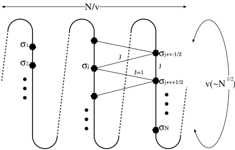
Figure 1: Imposing the screw-boundary condition Novotny90 ; Novotny92 , we construct the finite-size cluster for the triangular-lattice quantum Ising ferromagnet (2) with $N$ spins. As indicated above, the Ising spins constitute a $d=1$-dimensional alignment $\{\sigma_{i}\}$ ($i=1,2,\dots,N$), and the dimensionality is lifted to $d=2$ by the bridges (long-range interactions) over the $(v\pm 1/2)$-th-neighbor pairs ($v\approx\sqrt{N}$). The simulation algorithm is presented in Sec. II.1.

Here, the Pauli matrices $\{\vec{\sigma}_{i}\}$ are placed at each triangular-lattice points $i(\leq N)$, and the summation $\sum_{\langle ij\rangle}$ runs over all possible nearest-neighbor pairs $\langle ij\rangle$. The parameters $\Gamma$ and $H$ denote the transverse- and longitudinal-magnetic fields, respectively. Upon increasing $\Gamma$, there occurs a phase transition separating the ferromagnetic and paramagnetic phases. This phase transition belongs to the same universality class as that of the three-dimensional classical Ising model. The ground-state eigenvector $|\Gamma H\rangle$ was evaluated with the numerical diagonalization method. We imposed the screw-boundary condition Novotny90 ; Novotny92 in order to construct the finite-size cluster with an arbitrary number of spins, $N=14,16,\dots,32$; see Fig. 1.

As mentioned above, the aim of this paper is to investigate the critical behaviors of the transverse- and longitudinal-field fidelity susceptibilities around the critical point $\Gamma=\Gamma_{c}$ ($H=0$). The transverse-field fidelity susceptibility is defined by

$$\chi_{F}^{(t)}=\frac{1}{N}\left.\partial^{2}_{\Delta\Gamma}F\right|_{\Delta\Gamma=H=0}\sim|\Gamma-\Gamma_{c}|^{-\alpha_{F}^{(t)}},$$ (3)

with an extended fidelity $F(\Delta\Gamma,H)=|\langle\Gamma,H=0|\Gamma+\Delta\Gamma,H\rangle|$. The critical exponent $\alpha_{F}^{(t)}$ was estimated as $\alpha_{F}^{(t)}=0.73$ Yu09 and $0.715(20)$ Nishiyama13 with the numerical diagonalization method for the quantum Ising ferromagnet on the square lattice. A large-scale quantum-Monte-Carlo simulation for the finite-temperature fidelity susceptibility yields $\alpha_{F}^{(t)}=0.750(6)$ Albuquerque10 . On the contrary, little attention has been paid to the longitudinal component of the fidelity susceptibility

$$\chi_{F}^{(h)}=\frac{1}{N}\left.\partial^{2}_{H}F\right|_{\Delta\Gamma=H=0}\sim|\Gamma-\Gamma_{c}|^{-\alpha_{F}^{(h)}},$$ (4)

with the critical exponent $\alpha_{F}^{(h)}$. The critical indices $\alpha_{F}^{(t)}$ and $\alpha_{F}^{(h)}$ are independent, and suffice for obtaining conventional critical indices such as $\nu$ and $\gamma$. In this paper, we analyze the critical behavior of the $d=2$ quantum Ising ferromagnet, Eq. (2), via $\chi_{F}^{(t)}$ and $\chi_{F}^{(h)}$. According to Ref. Yu09 , the transverse-field fidelity susceptibility $\chi_{F}^{(t)}$ is less influenced by scaling corrections (the leading singularity $\sim|\Gamma-\Gamma_{c}|^{-\alpha_{F}^{(t)}}$ is dominating), and an analysis of the slope of the $\ln N$-$\ln\chi_{F}^{(t)}|_{\Gamma=\Gamma_{c}}$ plot is sufficient to determine $\alpha_{F}^{(t)}$ reliably as a preliminary survey. In this paper, we pursue this idea, considering (presumably minor) scaling corrections explicitly for both transverse and longitudinal components in a unified manner.

The rest of this paper is organized as follows. In Sec. II, we present the numerical results. The simulation algorithm is presented as well. In Sec. III, we address the summary and discussions.

II Numerical results

In this section, we present the numerical results for the $d=2$ quantum Ising model (2). We implement the screw-boundary condition, namely, Novotny’s method Novotny90 ; Novotny92 , to treat a variety of system sizes $N=14,16,\dots,32$ systematically; see Fig. 1. The linear dimension $L$ of the cluster is given by

$$L=\sqrt{N},$$ (5)

because $N$ spins constitute a rectangular cluster.

II.1 Simulation method: Screw-boundary condition

In this section, we explain the simulation scheme (Novotny’s method) Novotny90 ; Novotny92 to implement the screw-boundary condition; see Fig. 1.

To begin with, we sketch a basic idea of Novotny’s method. We consider a finite-size cluster as shown in Fig. 1. We place an $S=1/2$ spin (Pauli operator $\vec{\sigma}_{i}$) at each lattice point $i(\leq N)$. Basically, the spins constitute a one-dimensional ($d=1$) structure. The dimensionality is lifted to $d=2$ by the long-range interactions over the $(v\pm 1/2)$-th-neighbor distances ($v\approx\sqrt{N}$). Owing to the long-range interaction, the $N$ spins form a $\sqrt{N}\times\sqrt{N}$ rectangular network effectively.

We explain a number of technical details. First, the present simulation algorithm is based on Sec. 2 of Ref. Nishiyama11 . A slight modification has to be made in order to incorporate the longitudinal-field term, which is missing in the formalism of Ref. Nishiyama11 . To cope with this extra contribution, we put a term $-H\sum_{i}\sigma^{x}_{i}$ into Eq. (3) of Ref. Nishiyama11 . Last, as claimed in Ref. Nishiyama11 , the screw pitch $v(\approx\sqrt{N})$ was finely tuned to optimize the finite-size behavior. The optimized $v$ suppresses an oscillatory deviation inherent in the screw-boundary condition; an improvement over a predecessor Nishiyama13 is demonstrated clearly in Fig. 2. The list of the optimized $v$ is presented in Eq. (6) of Ref. Nishiyama11 . The choice of the lattice structure (triangular lattice) may also contribute to the improvement of the finite-size behavior, because the triangular lattice has higher rotational symmetry.

II.2 Analysis of the critical point $\Gamma_{c}$ via $\chi_{F}^{(t)}$

In Fig. 2, we present the transverse-field fidelity susceptivity $\chi_{F}^{(t)}$ (3) for various $\Gamma$, $N=14,16,\dots,32$, and $H=0$. A notable signature of criticality appears around $\Gamma_{c}\approx 4.3$; this critical point separates the paramagnetic ($\Gamma<\Gamma_{c}$) and ferromagnetic ($\Gamma>\Gamma_{c}$) phases.

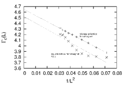
Figure 3: The approximate critical point $\Gamma_{c}(L)$ (plusses) [Eq. (6)] is plotted for $1/L^{2}$. The least-squares fit to these data yields $\Gamma_{c}=4.6478(50)$ in the thermodynamic limit $L\to\infty$. As a comparison, the approximate critical point for the square-lattice ferromagnet (crosses) Nishiyama13 (rather than that of the triangular lattice) is presented; the data are multiplied by a constant factor $\times 1.5$. For the latter model, there emerges an oscillatory deviation, which prohibits us from taking the thermodynamic limit reliably; such an oscillatory behavior is an artifact of the screw-boundary condition Novotny90 . In this paper, the triangular lattice is considered in order to suppress such a lattice artifact; details of the simulation technique are explained in Sec. II.1.

In Fig. 3, we plot the approximate critical point $\Gamma_{c}(L)$ (plusses) for $1/L^{2}$ ($N=14,16,\dots,32$). Here, the approximate critical point $\Gamma_{c}(L)$ denotes the location of maximal $\chi_{F}^{(t)}$ for each $L$; namely, the relation

$$\partial_{\Gamma}\chi_{F}^{(t)}(L)|_{\Gamma=\Gamma_{c}(L)}=0,$$ (6)

holds. The least-squares fit to the data in Fig. 3 yields an estimate $\Gamma_{c}=4.6478(50)$ in the thermodynamic limit $L\to\infty$. In a preliminary survey Nishiyama11 , the critical point is estimated as $\Gamma_{c}\approx 4.6$; see Fig. 4 of Ref. Nishiyama11 . This extrapolated critical point is no longer used in the subsequent analyses; rather, the approximate critical point $\Gamma_{c}(L)$ is fed into the formulas, (7) and (9).

As a comparison, we made a similar analysis for the square-lattice model Nishiyama13 (rather than the triangular lattice), and the approximate critical point $\Gamma_{c}(L)$ (crosses) is presented in Fig. 3; these data are multiplied by a constant factor $\times 1.5$. These data suffer from an oscillatory deviation inherent in the screw-boundary condition Novotny90 . That is, for quadratic values of $N\approx 16$, $25$, the deviation becomes suppressed. This notorious deviation seems to be eliminated satisfactorily for the present data in Fig. 3. Encouraged by this improvement, we analyze the power-law singularities of $\chi_{F}^{(t),(h)}$ in the next section.

II.3 Power-law singularities of the fidelity susceptibilities $\chi_{F}^{(t),(h)}$

In this section, we analyze the power-law singularities for the fidelity susceptibilities. According to the finite-size-scaling theory, at $\Gamma=\Gamma_{c}$, the fidelity susceptibilities $\chi_{F}^{(t),(h)}$ should obey the power law $\sim L^{\alpha_{F}^{(t),(h)}/\nu}$ with the correlation-length critical exponent $\nu$; see Ref. Gu11 . It has to be mentioned that as for the $d=1$ quantum Ising model, a thorough consideration of the finite-size scaling is presented in Ref. Ramski11 ; note that the $d=1$ counterpart is exactly solvable, and the results for considerably large $L$ are available. Moreover, an extended $d=1$ quantum Ising model was analyzed in Ref. Zhou08b , where the Ising universality was confirmed.

In Fig. 4, we plot the approximate critical exponent $\alpha_{F}^{(t)}/\nu(L_{1},L_{2})$ for $[2/(L_{1}+L_{2})]^{2}$ with $14\leq N_{1}<N_{2}\leq 32$ ($L_{1,2}=\sqrt{N_{1,2}}$). The approximate critical exponent is defined by

$$\frac{\alpha_{F}^{(t)}}{\nu}(L_{1},L_{2})=\frac{\ln\chi_{F}^{(t)}(L_{1})|_{\Gamma=\Gamma_{c}(L_{1})}-\ln\chi_{F}^{(t)}(L_{2})|_{\Gamma=\Gamma_{c}(L_{2})}}{\ln(L_{1}/L_{2})}.$$ (7)

The least-squares fit to the data in Fig. 4 yields $\alpha_{F}^{(t)}/\nu=1.205(62)$ in the thermodynamic limit $L\to\infty$. As a reference, we made a similar analysis with the abscissa scale replaced with $[2/(L_{1}+L_{2})]^{3}$. Thereby, we arrive at $\alpha_{F}^{(t)}/\nu=1.167(42)$. This result lies within the error margin, supporting the validity of the former result. As a conclusion, we estimate

$$\alpha_{F}^{(t)}/\nu=1.205(62).$$ (8)

This is a good position to address a number of remarks. First, the present estimate, Eq. (8), is slightly larger than the preceding ones, $\alpha_{F}^{(t)}/\nu=1.02$ Yu09 and $1.113(49)$ Nishiyama13 . Such a tendency toward enhancement should be attributed to the slight negative slope (finite-size drift) in Fig. 4. The validity of the present extrapolation scheme is examined in the next section, where a comparison with the existing values is made. Nevertheless, it is suggested that as for $\chi_{F}^{(t)}$, the leading singularity $\sim|\Gamma-\Gamma_{c}|^{-\alpha_{F}^{(t)}}$ is dominating, and a naive analysis without the $L\to\infty$ extrapolation admits an estimate satisfactory as a preliminary survey. Last, the data in Fig. 4 scatter intermittently around $[2/(L_{1}+L_{2})]^{2}\approx 0.033$ and $0.055$, namely, $L_{1,2}\approx 5.5$ and $4.5$. Such an irregularity is inherent in the screw-boundary condition Novotny90 ; the finite-size behavior exhibits an oscillatory deviation depending on the condition whether the system size $L$ is close to an integer or not. Here, we did not discard irregular data so as to exclude arbitrariness in the data analysis.

We turn to the analysis of the longitudinal-field fidelity susceptibility (4). In Fig. 5, we plot the approximate critical exponent $\alpha_{F}^{(h)}/\nu(L_{1},L_{2})$ for $[2/(L_{1}+L_{2})]^{2}$ with $14\leq N_{1}<N_{2}\leq 32$. The approximate critical exponent is defined by

$$\frac{\alpha_{F}^{(h)}}{\nu}(L_{1},L_{2})=\frac{\ln\chi_{F}^{(h)}(L_{1})|_{\Gamma=\Gamma_{c}(L_{1})}-\ln\chi_{F}^{(h)}(L_{2})|_{\Gamma=\Gamma_{c}(L_{2})}}{\ln(L_{1}/L_{2})}.$$ (9)

As mentioned above, an abrupt irregularity around $[2/(L_{1}+L_{2})]^{2}\approx 0.033$ and $0.055$ is an artifact of the screw-boundary condition. The least-squares fit to the data in Fig. 5 yields $\alpha_{F}^{(h)}/\nu=2.909(80)$. As a reference, we made a similar analysis with the abscissa scale replaced with $[2/(L_{1}+L_{2})]^{3}$. Thereby, we obtain $\alpha_{F}{(h)}/\nu=2.700(53)$. The discrepancy $\approx 0.2$ between different extrapolation schemes seems to be larger than that of the least-squares-fit error $\approx 0.08$; in fact, the slope (finite-size drift) of Fig. 5 is larger than that of Fig. 4. Regarding the discrepancy as an indicator of the error margin, we estimate the critical exponent as

$$\alpha_{F}^{(h)}/\nu=2.9(2).$$ (10)

II.4 Analysis of critical exponents: $\alpha_{F}^{(t)}$, $\alpha_{F}^{(h)}$, $\nu$, and $\gamma$

In the above section, we estimated the critical indices $\alpha_{F}^{(t)}/\nu$, Eq. (8), and $\alpha_{F}^{(h)}/\nu$ , Eq. (10). In this section, we estimate $\alpha_{F}^{(t)}$ and $\alpha_{F}^{(h)}$, separately, through resorting to the scaling relations. As a byproduct, we also provide the estimates for $\nu$ and $\gamma$; here, the index $\gamma$ denotes the critical exponent for the uniform-magnetic-field susceptibility.

Based on the results, Eqs. (8) and (10), we estimate the critical indices

$$\alpha_{F}^{(t)}=0.752(24)$$ (11)

and

$$\alpha_{F}^{(h)}=1.81(13).$$ (12)

Here, we utilized the scaling relations Albuquerque10

$$\alpha_{F}^{(t)} = \alpha+\nu$$ (13)

$$\alpha_{F}^{(h)} = \gamma+\nu.$$ (14)

The index $\alpha$ denotes the specific-heat critical exponent, which satisfies the hyper-scaling relation $\alpha=2-D\nu$ with the spatial and temporal dimensionality $D(=d+1)=3$. (As mentioned above, the $D=2$ Ising universality was analyzed extensively in Ref. Zhou08b .) These scaling relations are closed. Hence, we are able to calculate conventional critical indices

$$(\nu,\gamma)=[0.624(12),1.19(13)].$$ (15)

(Note that the $d=2$ quantum Ising model belongs to the same universality class as that of the $d=3$ classical Ising model.) We stress that critical indices are mutually dependent through scaling relations, and the set of exponents, Eq. (15), is sufficient for inspecting the validity of our analyses.

As for $\alpha_{F}^{(t)}$, our result, Eq. (11), is comparable with the preceding numerical-diagonalization results, $\alpha_{F}^{(t)}=0.73$ Yu09 and $0.715(20)$ Nishiyama13 . As mentioned in Sec. II.3, our result is slightly larger than these preceeding ones possibly because of the finite-size drift (negative slope) shown in Fig. 4. Actually, a large-scale-quantum-Monte-Carlo result $\alpha_{F}^{(t)}=0.750(6)$ for $N\leq 48\times 48$ Albuquerque10 seems to support the present extrapolation scheme.

To the longitudinal component of the fidelity susceptibility, little attention has been paid. Instead, we turn to consider the traditional critical indices $(\nu,\gamma)$ to examine a reliability of our analyses. According to the large-scale Monte Carlo simulation for the classical $d=3$ Ising model Deng03 , the set of critical exponents was estimated as $(\nu,\gamma)=[0.63020(12),1.23721(27)]$. Additionally, the above-mentioned quantum-Monte-Carlo simulation via $\chi_{F}^{(t)}$ readily yields the first component $\nu=0.625(3)$ Albuquerque10 . These results seem to support ours, Eq. (15). In other words, scaling corrections are appreciated properly through the extrapolation schemes in Figs. 4 and 5.

III Summary and discussions

The critical behaviors of the transverse- and longitudinal-field fidelity susceptibilities, Eqs. (3) and (4), for the triangular-lattice quantum Ising ferromagnet (2) were investigated with the numerical diagonalization method. We imposed the screw-boundary condition (Sec. II.1) in order to construct the finite-size cluster flexibly with an arbitrary number of constituent spins $N=14,16,\dots,32$.

We estimated the critical indices as $\alpha_{F}^{(t)}=0.752(24)$, Eq. (11), and $\alpha_{F}^{(h)}=1.81(13)$, Eq. (12), for the transverse- and longitudinal-field fidelity susceptibilities, respectively. As a byproduct, we obtained the conventional critical indices, $(\nu,\gamma)=[0.624(12),1.19(13)]$, Eq. (15). As for the transverse-field fidelity susceptibility, there have been reported a number of pioneering studies. By means of the numerical diagonalization method, the critical exponent was estimated as $\alpha_{F}^{(t)}=0.73$ Yu09 and $0.715(20)$ Nishiyama13 . A slight (seemingly systematic) deviation from ours should be attributed to the finite-size drift (negative slope) shown in Fig. 4. In fact, the quantum-Monte-Carlo simulation for $N\leq 48\times 48$ provides convincing evidence, $\alpha_{F}^{(t)}=0.750(6)$ Albuquerque10 , to validate the extrapolation scheme employed in Fig. 4. So far, little attention has been paid to the longitudinal component $\alpha_{F}^{(h)}$. Through resorting the scaling relations (Sec. II.4), one is able to estimate the conventional indices $(\nu,\gamma)$ straightforwardly from the pair of $\alpha_{F}^{(t)}$ and $\alpha_{F}^{(h)}$. The set of indices was estimated as $(\nu,\gamma)=[0.63020(12),1.23721(27)]$ with the large-scale Monte Carlo simulation for the three-dimensional classical Ising model Deng03 . Again, it is suggested that the scaling corrections are appreciated properly by the extrapolation schemes in Figs. 4 and 5. In other words, the finite-size scaling analysis via $\chi_{F}^{(t),(h)}$ is less influenced by corrections to scaling, and even for restricted system sizes, the critical indices are estimated reliably.

As mentioned in the Introduction, the fidelity susceptibilities are readily calculated with the numerical diagonalization method, with which an explicit expression for the ground state eigenvector is available. It would be tempting to apply the fidelity susceptibilities to a wide class of systems of current interest such as the frustrated quantum magnetism, for which the Monte Carlo method suffers from the negative-sign problem. This problem would be addressed in the future study.

Figure 2: The transverse-field fidelity susceptibility $\chi_{F}^{(t)}$ (3) is plotted for various $\Gamma$, $N=14,16,\dots,32$, and $H=0$. A notable signature of criticality emerges around $\Gamma_{c}\approx 4.3$. The finite-size drift of $\Gamma_{c}$ is analyzed in Fig. 3.

Figure 4: The approximate critical exponent $\alpha_{F}^{(t)}/\nu(L_{1},L_{2})$ (7) is plotted for $[2/(L_{1}+L_{2})]^{2}$ with $14\leq N_{1}<N_{2}\leq 32$ ($L_{1,2}=\sqrt{N_{1,2}}$). The least-squares fit to these data yields $\alpha_{F}^{(t)}/\nu=1.205(62)$ in the thermodynamic limit $L\to\infty$.

Figure 5: The approximate critical exponent $\alpha_{F}^{(h)}/\nu(L_{1},L_{2})$ (9) is plotted for $[2/(L_{1}+L_{2})]^{2}$ with $14\leq N_{1}<N_{2}\leq 32$ ($L_{1,2}=\sqrt{N_{1,2}}$). The least-squares fit to these data yields $\alpha_{F}^{(h)}/\nu=2.909(80)$ in the thermodynamic limit $L\to\infty$. A possible systematic error is considered in the text.

References

- (1) A. Uhlmann, Rep. Math. Phys. 9, 273 (1976).
- (2) R. Jozsa, J. Mod. Opt. 41, 2315 (1994).
- (3) A. Peres, Phys. Rev. A 30, 1610 (1984).
- (4) T. Gorin, T. Prosen, T. H. Seligman, and M. Žnidarič, Phys. Rep. 435, 33 (2006).
- (5) H. T. Quan, Z. Song, X. F. Liu, P. Zanardi, and C. P. Sun, Phys. Rev. Lett. 96, 140604 (2006).
- (6) P. Zanardi and N. Paunković, Phys. Rev. E 74, 031123 (2006).
- (7) H.-Q. Zhou, and J. P. Barjaktarevic̃, J. Phys. A: Math. Theor. 41, 412001 (2008).
- (8) V. R. Vieira, J. Phys: Conference Series 213, 012005 (2010).
- (9) H.-Q. Zhou, R. Orús, and G. Vidal, Phys. Rev. Lett. 100, 080601 (2008).
- (10) D. Schwandt, F. Alet, and S. Capponi, Phys. Rev. Lett. 103, 170501 (2009).
- (11) A. F. Albuquerque, F. Alet, C. Sire, and S. Capponi, Phys. Rev. B 81, 064418 (2010).
- (12) C. De Grandi, A. Polkovnikov, and A. W. Sandvik, Phys. Rev. B 84, 224303 (2011).
- (13) M.A. Novotny, J. Appl. Phys. 67, 5448 (1990).
- (14) M.A. Novotny, Phys. Rev. B 46, 2939 (1992).
- (15) W.-C. Yu, H.-M. Kwok, J. Cao, and S.-J. Gu, Phys. Rev. E 80, 021108 (2009).
- (16) Y. Nishiyama, to appear Physica A; arXiv:1305.3958.
- (17) Y. Nishiyama, J. Stat. Mech.: Theory and Experiment, P08020 (2011).
- (18) S.-J. Gu, H.-M. Kwok, W.-Q. Ning, and H.-Q. Lin, Phys. Rev. B 77, 245109 (2008); ibid. 83, 159905(E) (2011).
- (19) M.M. Rams and B. Damski, Phys. Rev. Lett. 106, 055701 (2011).
- (20) H.-Q. Zhou, J.-H. Zhao, and B. Li, J. Phys. A: Math. Theor. 41, 492002 (2008).
- (21) Y. Deng and H. W. J. Blöte, Phys. Rev. E 68, 036125 (2003).