Oriented Event Shapes at N³LL + $\mathcal{O}(\alpha_{\rm S}^{2})$

Abstract

We analyze oriented event-shapes in the context of Soft-Collinear Effective Theory (SCET) and in fixed-order perturbation theory. Oriented event-shapes are distributions of event-shape variables which are differential on the angle $\theta_{T}$ that the thrust axis forms with the electron–positron beam. We show that at any order in perturbation theory and for any event shape, only two angular structures can appear: $F_{0}=3/8\,(1+\cos^{2}\theta_{T})$ and $F_{1}=(1-3\,\cos^{2}\theta_{T})$. When integrating over $\theta_{T}$ to recover the more familiar event-shape distributions, only $F_{0}$ survives. The validity of our proof goes beyond perturbation theory, and hence only these two structures are present at the hadron level. The proof also carries over massive particles. Using SCET techniques we show that singular terms can only arise in the $F_{0}$ term. Since only the hard function is sensitive to the orientation of the thrust axis, this statement applies also for recoil-sensitive variables such as Jet Broadening. We show how to carry out resummation of the singular terms at N³LL for Thrust, Heavy-Jet Mass, the sum of the Hemisphere Masses and $C$-parameter by using existing computations in SCET. We also compute the fixed-order distributions for these event-shapes at $\mathcal{O}(\alpha_{\rm S})$ analytically and at $\mathcal{O}(\alpha_{\rm S}^{2})$ with the program Event2.

1 Introduction

The experimental collaborations at LEP collected very precise data for event-shape distributions at the $Z$-pole energy (LEP1) and also at higher energies (LEP2) with somewhat larger uncertainties. These data, along with measurements at lower energies from other experiments, have been recently analyzed for the thrust distribution Abbate:2010xh ; Gehrmann:2012sc and moments Gehrmann:2009eh ; Abbate:2012jh using higher-order resummation, three-loop matrix elements and analytic methods to parametrize non-perturbative power corrections. These analyses found rather low values of the strong coupling $\alpha_{\rm S}$ with quite small uncertainties, which are in disagreement with the world average PDG:2012  . Further analysis for $C$-parameter and Heavy-Jet Mass are on the way Hoang:2013 ; Hoang:2013a .

These analyses, and the vast majority of the experimental activity, have focused only on angular-averaged event-shapes. By averaged we want to stress the fact that there was no information recorded on the orientation of the event with respect to the beam axis. The DELPHI collaboration delivered Abreu:2000ck very accurate measurements of eighteen oriented infrared and collinear safe observables at the $Z$-peak from $1.5$ million collected events. Oriented distributions are differential in the event-shape variable, as usual, but also on the polar angle formed by the thrust axis and the beam direction, see Fig. 1 (events are symmetric with respect to the azimuthal angle and hence its dependence is integrated). They also presented a very accurate determination of $\alpha_{\rm S}$ by performing two-parameter fits to $\alpha_{\rm S}$ and $x_{\mu}$, the square of the ratio between the renormalization scale $\mu$ and the center-of-mass energy $Q$. Data was compared to ${\mathcal{O}}(\alpha_{\rm S}^{2})$ theoretical computations Catani:1996jh ; Catani:1996vz ; Rodrigo:1997gy , neglecting QED corrections. Even though they analyzed the effect of NLL resummation, their main analysis relies on fixed-order perturbation theory.

The OPAL collaboration also performed oriented measurements with respect to the thrust axis for both the total cross section and the thrust distribution from $2.1$ million collected events Abbiendi:1998at . Data were presented at the hadron and parton level, corrected with Monte Carlo generators.

In this article we take a first step towards an analysis which uses the most recent theoretical developments: ${\mathcal{O}}(\alpha_{\rm S}^{3})$ matrix elements GehrmannDeRidder:2007bj ; GehrmannDeRidder:2007hr ; Weinzierl:2008iv ; Weinzierl:2009ms and higher-order log resummation. We also show how to treat oriented distributions in a more systematic fashion, demonstrating that there is only one additional piece of information as compared to averaged event-shapes. We compute this new piece analytically at ${\mathcal{O}}(\alpha_{\rm S})$ and extract it numerically at ${\mathcal{O}}(\alpha_{\rm S}^{2})$ using Event2 Catani:1996jh ; Catani:1996vz . We also proof that singular logs can only occur in the angular averaged piece. Fixed-order computations of oriented event-shapes at $\mathcal{O}(\alpha_{s})$ fully differential and for thrust were presented in Ref. Lampe:1992au , together with a numerical determination of the $\mathcal{O}(\alpha_{s}^{2})$ contribution to the integrated longitudinal cross section; an SCET factorization theorem for the longitudinal piece of the thrust distribution was derived in Hagiwara:2010cd , achieving NLL resummation (this term is subleading in the SCET counting). In this article we derive the singular behavior of the various angular structures directly from SCET, without assuming a splitting in transverse and longitudinal parts.

A thorough comparison to experimental data including ${\mathcal{O}}(\alpha_{\rm S}^{3})$ matrix elements, QED and bottom-quark mass effects along with non-perturbative power corrections is left for future work.

The event-shape variables that we consider in this article are:

1. Thrust Farhi:1977sg  :
   Thrust is defined as the sum of the absolute values of the projections of each particle three-momentum on a given direction $\hat{n}$. This direction is chosen such that the sum is maximized, and the result is then normalized to the sum of the magnitudes of the three-momenta of all particles 

   $$T=1-\tau=\dfrac{1}{\sum_{i}|\vec{p}_{i}|}\max_{\hat{n}}\sum_{i}|{\hat{n}}\cdot{\vec{p}}_{i}|\,.$$ (1)

   It is customary to define $\tau=1-T$, since as $\tau\to 0$ one reaches the dijet limit. For simplicity we will use the name thrust also for $\tau$.

2. $C$-parameter Parisi:1978eg ; Donoghue:1979vi  :
   Unlike thrust, $C$-parameter does not require any minimization procedure. It is defined in terms of the eigenvalues of the linearized momentum tensor. It can be written as a double sum over the three-momenta magnitudes and relative angle of pairs of particles, normalized analogously to thrust 

   $$C=\frac{3}{2}\frac{\sum_{i,j}|\vec{p}_{i}||\vec{p}_{j}|\sin^{2}\theta_{ij}}{\left(\sum_{i}|\vec{p}_{i}|\right)^{2}}\,.$$ (2)

3. Hemisphere Masses Clavelli:1979md ; Chandramohan:1980ry ; Clavelli:1981yh  :
   The plane normal to the thrust axis $\hat{n}$ defines two separated hemispheres (see Fig. 1) which shall be denoted by $a$ and $b$. The hemisphere masses are defined as the square of the total four-momentum in each hemisphere

   $$S_{a,b}=\bigg{(}\sum_{i\in a,b}p_{i}^{\mu}\bigg{)}^{2}\,,$$ (3)

   One can define two dijet event-shapes out of the hemisphere masses, Heavy-Jet Mass $\rho$  and the sum of the hemisphere masses $\rho_{S}$, and the non-dijet event-shapes Light-Jet Mass $\rho_{L}$ and the absolute value of the difference of the hemisphere masses $\rho_{D}$, all of them normalized to the square of the center-of-mass energy $Q^{2}$

   $$\rho=\dfrac{1}{Q^{2}}\max(S_{a},S_{b})\,, \quad\quad\rho_{L}=\dfrac{1}{Q^{2}}\min(S_{a},S_{b})\,,$$ (4)

   $$\rho_{S}=\dfrac{S_{a}+S_{b}}{Q^{2}}=\rho+\rho_{L}\,, \quad\quad\rho_{D}=\dfrac{|S_{a}-S_{b}|}{Q^{2}}=\rho-\rho_{L}\,.$$

   The dijet configuration is achieved when both hemisphere masses are small. Heavy-Jet Mass is a dijet event-shape because when $\rho$ is small both hemisphere masses have to be small. The same goes true for $\rho_{S}$. However $\rho_{L}$ can be small when one hemisphere mass is big while the other is small, and $\rho_{D}$ can be small for big hemisphere masses but of similar size. There is a relation between the hemisphere masses and thrust and 2-jettiness:

   $$\tau =1-\dfrac{Q}{\sum_{i}|\vec{p}_{i}|}\sqrt{1-2\,\rho_{S}+\rho_{D}^{2}}~{},$$ (5)

   $$\tau_{2} =1-\sqrt{1-2\,\rho_{S}+\rho_{D}^{2}}~{}.$$

   Expanding at leading order in the dijet limit one has $\tau_{2}=\rho_{S}+{\mathcal{O}}(S_{a,b}^{2})$. The mass of a hemisphere is zero when it is populated by a single massless particle only, hence $\rho_{L}$ is zero for events with two or three massless particles. Plugging $\rho_{L}=0$ into Eqs. (4) and (5) one finds that thrust, $\rho$, $\rho_{S}$ and $\rho_{D}$ are identical for two and three (massless) particles. Hence the ${\mathcal{O}}(\alpha_{\rm S})$ fixed-order computation of Sec. 3 is the same for the three event-shapes, and we will present the results for thrust and $C$-parameter only. At NLO we will present results for $\tau$, $\rho$ and $\rho_{S}$, as well as for $C$-parameter.

This paper is organized as follows: In Sec. 2 we derive an all-orders factorization theorem for oriented event-shapes in Soft-Collinear Effective Theory (SCET) Bauer:2000ew ; Bauer:2000yr ; Bauer:2001ct ; Bauer:2001yt ; Bauer:2002nz , which permits resummation at N³LL; in Sec. 3 we compute the ${\mathcal{O}(\alpha_{\rm S})}$ fixed-order distribution for oriented event-shapes; in Sec. 4 we show that to all orders in perturbation theory and even at the hadronic level, only two angular structures can arise; in Sec. 5 we determine the ${\mathcal{O}(\alpha_{\rm S}^{2})}$ fixed-order distribution for some oriented distributions using Event2, along with the oriented total cross-section; conclusions and outlook can be found in Sec. 6.

2 SCET Factorization Theorem for Oriented Event-Shapes

In this section we derive the SCET factorization theorem for the most singular terms in the oriented event-shape distributions. Factorized expressions in SCET are tremendously useful as they a) allow to carry out resummation of large logarithms to very high accuracy through Renormalization Group Evolution (RGE); as is the case of thrust Becher:2008cf ; Abbate:2010xh , Heavy-Jet Mass Chien:2010kc ; Hoang:2013 , $C$-parameter Hoang:2013a at N³LL, Jet Broadening Rakow:1981qn at N²LL Becher:2011pf ; Becher:2012qc , or angularities Berger:2003iw ; Hornig:2009vb at NLL ; b) simplify the calculation of the necessary ingredients (matrix elements and anomalous dimensions); c) confine non-perturbative effects to specific functions Bauer:2002ie ; Bauer:2003di ; Mateu:2012nk . Factorization of event-shape cross-sections was first performed in QCD in Korchemsky:1998ev ; Korchemsky:1999kt ; Korchemsky:2000kp and was followed by Effective Field Theory techniques in Fleming:2007qr ; Schwartz:2007ib ; Hoang:2007vb . Recently subleading corrections to the thrust distribution have been derived in SCET Freedman:2013vya .

Our proof closely follows the derivation given in Ref. Bauer:2008dt and actually requires only minimal modifications. Let $p_{1}$ and $p_{2}$ be the four-momenta of the incoming electron and positron, respectively, and let $Q$ be the center-of-mass energy.  The leptonic tensor involved in the process $e^{+}e^{-}\to\rm hadrons$ can be split into vector and axial contributions, and is given by 

$$L_{V\,(A)}^{\mu\nu} =\dfrac{16\pi^{2}\alpha^{2}}{Q^{4}}\,\mathcal{V}^{\mu\nu}\,L_{V\,(A)}~{},$$ (6)

$$\mathcal{V}^{\mu\nu} =p_{1}^{\mu}p_{2}^{\nu}+p_{2}^{\mu}p_{1}^{\nu}-\dfrac{Q^{2}}{2}\,g^{\mu\nu}~{},$$

where $L_{V\,(A)}$ are electroweak factors which can be found for instance in Eq. (9) of Ref. Bauer:2008dt . Considering only QED interactions $L_{V}=\sum_{f}Q_{f}^{2}$ and $L_{A}=0$, being $f$ the quark flavor. In full QCD an event shape can be written as

$$~{}\dfrac{\mathrm{d}\sigma}{\mathrm{d}e} =\dfrac{1}{2Q^{2}}\!\int\mathrm{d}^{4}x\,e^{iq\cdot x}\sum_{i=V,A}L^{i}_{\mu\nu}\,\langle\,0\,|\,j_{i}^{\mu\,\dagger}(x)\,\delta(e-{\hat{e}})\,j_{i}^{\nu}(0)\,|\,0\,\rangle\,,$$ (7)

$$j_{i}^{\mu} =\bar{q}_{f}\,\Gamma_{i}^{\mu}\,q_{f}\,,\quad\Gamma_{V}^{\mu}=\gamma^{\mu}\,,\quad\Gamma_{A}^{\mu}=\gamma^{\mu}\gamma_{5}\,,$$

where $\hat{e}$ is an operator that when acting on a state pulls out as an eigenvalue the value of the event shape $e$ : $\hat{e}\,|\,X\,\rangle=e(X)\,|\,X\,\rangle$, and $i=V,A$ labels vector and axial currents. In the second line of Eq. (7) there is an implicit sum over the color of the quarks. In the rest of the proof we omit sums over the quark flavors, which can be trivially inferred. The next step is to match the QCD current $j_{i}^{\mu}$ onto SCET:

$$~{}j_{i}^{\mu} =\sum_{\hat{n}}\sum_{\tilde{p}_{1},\tilde{p}_{2}}C_{n,\bar{n}}(\tilde{p}_{1},\tilde{p}_{2},\mu)\,\mathcal{O}_{n\bar{n}}(x;\tilde{p}_{1},\tilde{p}_{2})\,,$$ (8)

$$\mathcal{O}_{n\bar{n}}(x;\tilde{p}_{1},\tilde{p}_{2}) =e^{i(\tilde{p}_{1}-\tilde{p}_{2})\cdot x}\,\bar{\chi}_{n,\tilde{p}_{1}}(x)Y_{n}(x)\Gamma_{i}^{\mu}\overline{Y}_{\bar{n}}(x)\chi_{{\bar{n}},{\tilde{p}}_{2}}\,.$$

$n^{\mu}$ and ${\bar{n}}^{\mu}$ are light-like vectors in the direction of the primary quark and anti-quark four-momenta. More specifically, if $\hat{n}$ is the direction of the thrust axis, then $n^{\mu}=(1,{\hat{n}})$, ${\bar{n}}^{\mu}=(1,-\,{\hat{n}})$, such that $n^{2}=\bar{n}^{2}=0$ and $n\cdot\bar{n}=2$. Since the SCET spinors have only two components one can simplify the Dirac matrices to $\Gamma_{V}^{\mu}=\gamma_{\perp}^{\mu}$ and $\Gamma_{A}^{\mu}=\gamma_{\perp}^{\mu}\gamma_{5}$, with $\gamma_{\perp}$ the projection of the Dirac matrices into the $x$ – $y$ plane: $\gamma_{\perp}^{\mu}\,=\,\gamma^{\mu}\,-\,n\!\!\!/\,\bar{n}^{\mu}/2\,-\,\bar{n}\!\!\!/\,n^{\mu}/2$. $Y_{n}$ and $\overline{Y}_{\bar{n}}$ are path- and anti-path orderer soft Wilson lines, respectively, in the corresponding light-like directions. $\chi$ represents a jet field, which is the product of a collinear quark field and a collinear Wilson line, making the combination collinear gauge invariant. $\tilde{p}_{j}$ are large label momenta (we use here the label formalism). In Eq. (8) we have used a field redefinition Bauer:2001yt that decouples soft and collinear degrees of freedom at leading order in the SCET Lagrangian. This is the first step to factorize the cross section.

Next one replaces Eq. (8) into (7) and requires label momentum conservation. This fixes $\bar{n}\cdot\tilde{p}_{1}=-\,n\cdot\tilde{p}_{2}=Q$ and makes the label transverse momenta zero. Then the hard function is defined as $H(Q,\mu)\equiv|C_{n,\bar{n}}(Q,Q,\mu)|^{2}$. In the next step towards factorization the event shape delta function is decomposed as follows:

$$\delta(e-{\hat{e}})=\!\int\mathrm{d}e_{n}\,\mathrm{d}e_{\bar{n}}\,\mathrm{d}e_{s}\,\delta(e_{n}-\hat{e}_{n})\,\delta(e_{\bar{n}}-\hat{e}_{\bar{n}})\,\delta(e_{s}-\hat{e}_{s})\,\delta(e-e_{n}-e_{\bar{n}}-e_{s})\,,$$ (9)

where $\hat{e}_{n}$, $\hat{e}_{\bar{n}}$ and $\hat{e}_{s}$ are event-shape operators acting only on the $n$-, $\bar{n}$-collinear and soft sectors, respectively. Then, color conservation and the Fierz identity for Dirac matrices are used to place next to one another fields belonging to the various sectors. After some manipulations of the various matrix elements, as detailed in Ref. Bauer:2008dt , one arrives at

$$\dfrac{\mathrm{d}\sigma}{\mathrm{d}e} =K_{0}\,H(Q,\mu)\sum_{\hat{n}}\dfrac{\mathrm{d}^{2}\vec{k}_{\perp}}{2(2\pi)^{2}}\!\int\!\mathrm{d}e_{n}\,\mathrm{d}e_{\bar{n}}\,\mathrm{d}e_{s}\,\delta(e-e_{n}-e_{\bar{n}}-e_{s})\,J_{n}(e_{n},\mu)\,J_{\bar{n}}(e_{\bar{n}},\mu)\,S_{e}(e_{s},\mu)\,,$$

$$K_{0} =\dfrac{N_{C}}{2Q^{2}}\!\sum_{i=V,A}L_{i}^{\mu\nu}\,{\rm Tr}\Big{[}\dfrac{\bar{n}\!\!\!/}{2}\,\Gamma_{i}^{\mu}\,\dfrac{n\!\!\!/}{2}\,\overline{\Gamma}_{i}^{\nu}\Big{]}\,,$$ (10)

where $J$ and $S$ are the jet and soft functions, respectively. Following Ref. Fleming:2007qr one can work out together the sum over $\hat{n}$ and the integral measure over the transverse momentum to find

$$\sum_{\hat{n}}\dfrac{\mathrm{d}^{2}\vec{k}_{\perp}}{2(2\pi)^{2}}=\dfrac{Q^{2}}{32\pi^{2}}\,\mathrm{d}\Omega\,.$$ (11)

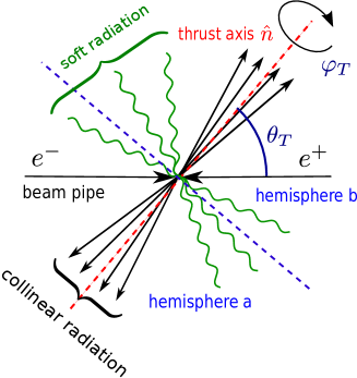
Figure 1: Schematic dijet event. The thrust axis is depicted as a dashed red line. Collinear particles are represented as black arrows around the thrust axis. Soft radiation appears as green wiggly lines and can be emitted in central regions of the phase-space. The two hemispheres $a$ and $b$ are separated by a plane normal to the thrust axis, and in this figure it appears as a blue dashed line. $\theta_{T}$ is defined as the angle between the beam (for example the initial-state electron) and the thrust axis. $\varphi_{T}$ is the orientation of the event in the azimuthal direction around the thrust axis. We average over that angle.

Here $\Omega$ refers to the orientation of the thrust axis with respect to the beam, as illustrated in Fig. 1. Finally, calculating the trace in Eq. (10) and collecting some factors, we find that the most singular contribution to the differential angular distribution of the event-shape $e$ is

$$\dfrac{1}{\sigma_{0}}\dfrac{\mathrm{d}\sigma_{\rm S}}{\mathrm{d}\Omega\,\mathrm{d}e}=\dfrac{3}{16\pi}\dfrac{1}{Q^{2}}(n_{\mu}{\bar{n}}_{\nu}+n_{\nu}{\bar{n}}_{\mu}-2g_{\mu\nu})\mathcal{V}^{\mu\nu}\dfrac{1}{\sigma_{0}}\dfrac{\mathrm{d}\sigma_{\rm S}}{\mathrm{d}e}\,,$$ (12)

where

$$\sigma_{0}=\dfrac{4\pi\alpha^{2}N_{C}}{3Q^{2}}\,(L_{V}+L_{A})\,,$$ (13)

is the Born cross-section. It is straightforward to compute $(n_{\mu}{\bar{n}}_{\nu}+n_{\nu}{\bar{n}}_{\mu}-2g_{\mu\nu})\mathcal{V}^{\mu\nu}=Q^{2}(1+\cos^{2}\theta_{T})$, which leads to our final result:

$$\dfrac{1}{\sigma_{0}}\dfrac{\mathrm{d}\sigma_{\rm S}}{\mathrm{d}\!\cos\theta_{T}\,\mathrm{d}e}=\dfrac{3}{8}\,(1+\cos^{2}\theta_{T})\,\dfrac{1}{\sigma_{0}}\dfrac{\mathrm{d}\sigma_{\rm S}}{\mathrm{d}e}\,.$$ (14)

The form of Eq. (14) is actually very simple: the most singular terms of the oriented event-shape distribution inherit the angular dependence of the lowest order process $e^{+}e^{-}\to q\,\bar{q}$, shown in Fig. 2, identifying the thrust axis with the direction of the produced quark. The structure of singular logarithms and power corrections is completely identical to that of averaged event-shapes. Terms with any other angular dependence cannot contain singular terms. We will explicitly verify this at $\mathcal{O}(\alpha_{\rm S})$ (analytically) in Sec. 3 and at $\mathcal{O}(\alpha_{\rm S}^{2})$ (numerically) in Sec. 5. The same result was found in Fleming:2007xt for the case of doubly differential hemisphere mass distribution.

We close this section by showing the explicit factorized form of the averaged event-shape distribution Bauer:2008dt

$$\dfrac{1}{\sigma_{0}}\dfrac{\mathrm{d}\sigma_{\rm S}}{\mathrm{d}e}=H(Q,\mu)\!\int\!\mathrm{d}e_{n}\,\mathrm{d}e_{\bar{n}}\,\mathrm{d}e_{s}J_{n}(e_{n},\mu)\,J_{\bar{n}}(e_{\bar{m}},\mu)\,S(e_{s},\mu)\,\delta(e-e_{s}-e_{n}-e_{\bar{n}})\,.$$ (15)

The dominant non-perturbative effects are encoded in the soft function. The jet functions describe collinear radiation (black arrows in Fig. 1) and the soft function describes large angle soft radiation (green wiggly lines in Fig. 1).

3 LO Distribution

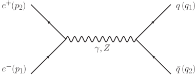
Figure 2: The ${\cal O}(\alpha_{\rm S}^{0})$ contribution to oriented event-shapes.

In this section we explicitly compute the oriented distribution at $\mathcal{O}(\alpha_{\rm S}^{0})$ and $\mathcal{O}(\alpha_{\rm S})$ for any event-shape. Let us start with the tree-level result, which we know is purely singular, and hence from the main result of Sec. 2 is expected to be proportional to $1+\cos^{2}\theta_{T}$. The diagram to be computed is shown in Fig. 2. In this case the thrust axis is obviously aligned with the direction of the (anti-)quark, and the event-shape variable can only take its lowest order value. For most event-shapes this value is simply $0$. Accordingly one only needs to compute the differential cross-section in $\cos\theta_{T}$ and multiply the result by $\delta(e)$. We find

$$\dfrac{1}{\sigma_{0}}\dfrac{\mathrm{d}\sigma^{0}}{\mathrm{d}\!\cos\theta_{T}\,\mathrm{d}e}\,=\,\dfrac{3}{8}\,(1+\cos^{2}\theta_{T})\,\delta(e)\,.$$ (16)

The first non-trivial computation appears at $\mathcal{O}(\alpha_{\rm S})$. It is nevertheless possible to carry out analytically the projection to $\cos\theta_{T}$. The final projection to any particular event-shape can be performed afterwards in the usual fashion. For this exercise, as a first step we find it convenient to parametrize the phase-space in terms of the energies of the quark $E_{1}$ and anti-quark $E_{2}$ and two out of the three angles formed by the incoming electron and the quark ($\theta_{1}$), the anti-quark ($\theta_{2}$) and the gluon ($\theta_{3}$). More specifically we define

$$E_{1}=\dfrac{Qx_{1}}{2}\,,\qquad E_{2}=\dfrac{Qx_{2}}{2}\,,$$ (17)

$$x_{1}+x_{2}+x_{3}=2\,,$$

$$x_{1}\cos\theta_{1}+x_{2}\cos\theta_{2}+x_{3}\cos\theta_{3}=0\,,$$

as it is customary. The second line in (17) follows from energy conservation, the last line from three-momentum conservation in the beam direction. Using these variables and adding the flux factor we find 

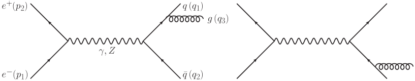
Figure 3: Leading order corrections at ${\cal O}(\alpha_{\rm S})$ to oriented event-shapes.

$$\dfrac{1}{2\,Q^{2}}\,\mathrm{d}\phi_{3}(P;q_{1},q_{2},q_{3}) =\dfrac{1}{512\,\pi^{3}}\,\mathrm{d}x_{1}\mathrm{d}x_{2}\,\mathrm{d}\!\cos\theta_{i}\,\mathrm{d}\!\cos\theta_{j}\,\theta(\sin^{2}\theta_{ij})\,h_{ij}^{-1/2}\,\theta(h_{ij})~{},$$

$$\cos\theta_{ij} =\dfrac{2x_{k}+x_{i}x_{j}-2}{x_{i}x_{j}}~{},$$

$$\sin\theta_{ij} =\dfrac{2}{x_{i}x_{j}}\sqrt{(1-x_{1})(1-x_{2})(1-x_{3})}~{},$$

$$h_{ij} =\sin^{2}\theta_{ij}-\cos^{2}\theta_{i}-\cos^{2}\theta_{j}+2\cos\theta_{ij}\cos\theta_{i}\cos\theta_{j}~{},$$ (18)

where $i\neq j\neq k$ take values $1$, $2$ or $3$. The function $h_{ij}$ can conveniently be written as

$$h_{ij}=(\cos\theta_{ij}^{+}-\cos\theta_{i})(\cos\theta_{i}-\cos\theta_{ij}^{-})~{},$$ (19)

$$\cos\theta_{ij}^{\pm}=\cos\theta_{ij}\cos\theta_{j}\,\pm\,\sin\theta_{ij}\sin\theta_{j}=\cos(\theta_{ij}\mp\theta_{j})~{}.$$

The only integrals involving $h_{ij}$ that one needs contain powers of $\cos^{n}\theta_{i}$ that can be trivially solved

$$\int\!\mathrm{d}\!\cos\theta_{i}\,\mathrm{d}\!\cos\theta_{j}\,h_{ij}^{-1/2}\theta(h_{ij})\cos^{n}\theta_{i}=$$ (20)

$$\sqrt{\pi}\,\sum_{l=0}^{n}\binom{n}{l}\dfrac{(2\sin\theta_{ij}\sin\theta_{j})^{l}\cos^{n-l}\theta_{ij}^{+}}{l!}\,\Gamma\bigg{(}\dfrac{1}{2}+l\bigg{)}\,.$$

Computing the diagrams depicted in Fig. 3 we find

$$\dfrac{1}{\sigma_{0}}\dfrac{\mathrm{d}\sigma^{\rm LO}}{\mathrm{d}x_{1}\mathrm{d}x_{2}\mathrm{d}\!\cos\theta_{i}\mathrm{d}\!\cos\theta_{j}}=\dfrac{3\alpha_{\rm S}}{16\pi^{2}}\,C_{F}\,h_{ij}^{-1/2}\theta(h_{ij})\,\dfrac{(1+\cos^{2}\theta_{1})\,x_{1}^{2}+(1+\cos^{2}\theta_{2})\,x_{2}^{2}}{(1-x_{1})(1-x_{2})}\,.$$ (21)

Integrating over $\cos\theta_{1}$ and $\cos\theta_{2}$ we recover the averaged result of Ref. Ellis:1980nc

$$\dfrac{1}{\sigma_{0}}\dfrac{\mathrm{d}\sigma^{\rm LO}}{\mathrm{d}x_{1}\mathrm{d}x_{2}}=\dfrac{\alpha_{\rm S}}{2\pi}\,C_{F}\,\dfrac{x_{1}^{2}+x_{2}^{2}}{(1-x_{1})(1-x_{2})}\,.$$ (22)

The next step is to project Eq. (21) onto $\cos\theta_{T}$. This is achieved with the following projecting delta function:

$$\delta_{T}^{(3)} =\theta(x_{1}-x_{2})\,\theta(x_{1}-x_{3})\,\delta(\cos\theta_{T}-\cos\theta_{1})$$ (23)

$$+\,\theta(x_{2}-x_{1})\,\theta(x_{2}-x_{3})\,\delta(\cos\theta_{T}-\cos\theta_{2})$$

$$+\,\theta(x_{3}-x_{1})\,\theta(x_{3}-x_{2})\,\delta(\cos\theta_{T}-\cos\theta_{3})\,.$$

The regions delimited by the various pairs of $\theta$ functions are shown in Fig. 4. Let us define the polar-angle phase-space integral that projects onto the thrust axis as

$$\mathrm{d}\Phi_{ij}^{T}=\mathrm{d}\!\cos\theta_{i}\,\mathrm{d}\!\cos\theta_{j}\,h_{ij}^{-1/2}\theta(h_{ij})\,\delta_{T}^{(3)}~{}.$$ (24)

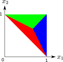
Figure 4: Regions of phase-space with a common thrust axis. In the blue (red) region the thrust axis points into the quark (anti-quark) three-momentum direction; in the green region the thrust axis points into the gluon momentum.

Then the projection of the three different angular-dependent pieces is straightforward:

$$\dfrac{1}{\pi}\int\!\mathrm{d}\Phi_{ij}^{T}= \,1\,,$$ (25)

$$\dfrac{1}{\pi}\int\!\mathrm{d}\Phi_{ij}^{T}\cos^{2}\theta_{1}= \,\cos^{2}\theta_{T}+\dfrac{1}{2}(1-3\cos^{2}\theta_{T})\bigg{[}\theta(x_{2}-x_{1})\,\theta(x_{2}-x_{3})\sin^{3}\theta_{12}$$

$$+\theta(x_{3}-x_{1})\,\theta(x_{3}-x_{2})\sin^{3}\theta_{13}\bigg{]}\,,$$

$$\dfrac{1}{\pi}\int\!\mathrm{d}\Phi_{ij}^{T}\cos^{2}\theta_{2}= \,\cos^{2}\theta_{T}+\dfrac{1}{2}(1-3\cos^{2}\theta_{T})\bigg{[}\theta(x_{1}-x_{2})\,\theta(x_{1}-x_{3})\sin^{3}\theta_{12}$$

$$+\theta(x_{3}-x_{1})\,\theta(x_{3}-x_{2})\sin^{3}\theta_{23}\bigg{]}\,.$$

Using the results of Eq. (25) in (21) we find

$$\dfrac{1}{\sigma_{0}}\dfrac{\mathrm{d}\sigma^{\rm LO}}{\mathrm{d}x_{1}\mathrm{d}x_{2}\,\mathrm{d}\!\cos\theta_{T}}=\dfrac{3}{8}\,(1+\cos^{2}\theta_{T})\,\dfrac{1}{\sigma_{0}}\dfrac{\mathrm{d}\sigma^{\rm LO}}{\mathrm{d}x_{1}\mathrm{d}x_{2}}+\dfrac{3\alpha_{\rm S}}{8\pi}\,C_{F}(1-3\cos^{2}\theta_{T})$$ (26)

$$\times(1-x_{3})\Bigg{[}\dfrac{\theta(x_{1}-x_{2})\,\theta(x_{1}-x_{3})}{x_{1}^{2}}+\dfrac{\theta(x_{2}-x_{1})\,\theta(x_{2}-x_{3})}{x_{2}^{2}}+\dfrac{2\,\theta(x_{3}-x_{1})\,\theta(x_{3}-x_{2})}{x_{3}^{2}}\Bigg{]}\,.$$

The second line in Eq. (26) is in agreement with the results of Ref. Lampe:1992au . Integrating over $\cos\theta_{T}$ one recovers the averaged result of Eq. (22). From Eq. (26) it is obvious that only the term proportional to $(1+\cos^{2}\theta_{T})$ can contain singular terms, as predicted by SCET in Eq. (14). Finally, when projected onto any event-shape $e$ one has the generic form

$$\dfrac{1}{\sigma_{0}}\dfrac{\mathrm{d}\sigma^{\rm LO}}{\mathrm{d}e\,\mathrm{d}\!\cos\theta_{T}}=\dfrac{3}{8}\,(1+\cos^{2}\theta_{T})\,\dfrac{1}{\sigma_{0}}\dfrac{\mathrm{d}\sigma^{\rm LO}}{\mathrm{d}e}+(1-3\cos^{2}\theta_{T})\,\dfrac{1}{\sigma_{0}}\dfrac{\mathrm{d}\sigma_{\rm ang}^{\rm LO}}{\mathrm{d}e}\,.$$ (27)

We shall demonstrate in Sec. 4 that the structure of Eq. (27) holds to any order in perturbation theory and even beyond perturbative QCD.

It turns out that the term proportional to $(1-3\cos^{2}\theta_{T})$ is much smaller that the one proportional to $(1+\cos^{2}\theta_{T})$. This is partially due to the fact that the former is purely non-singular while the latter has singular terms which numerically dominate. However, even if the singular terms are subtracted the second structure is at most $20\%$ ($15\%$ on average) of the first one. This behavior persists at higher orders.

As a final comment, one can calculate the total-oriented cross-section, completely inclusive in the final-state hadrons but still differential in the thrust direction. It again follows the pattern of Eq. (27):

$$\dfrac{1}{\sigma_{0}}\dfrac{\mathrm{d}\sigma}{\mathrm{d}\!\cos\theta_{T}}=\dfrac{3}{8}\,(1+\cos^{2}\theta_{T})\,R_{\rm had}+(1-3\cos^{2}\theta_{T})\,R_{\rm ang}\,,$$ (28)

$$R_{\rm had}=1+\dfrac{\alpha_{S}}{\pi}\,\dfrac{3\,C_{F}}{4}+\mathcal{O}(\alpha_{\rm S}^{2})=1+\dfrac{\alpha_{S}}{\pi}\,R_{1}^{\rm had}+\mathcal{O}(\alpha_{\rm S}^{2})\,,$$

$$R_{\rm ang}=\dfrac{\alpha_{\rm S}}{\pi}\,\dfrac{3\,C_{F}}{8}\,\Big{[}\,8\,\log\Big{(}\dfrac{3}{2}\Big{)}-3\,\Big{]}+\mathcal{O}(\alpha_{\rm S}^{2})=\dfrac{\alpha_{\rm S}}{\pi}\,R_{1}^{\rm ang}+\mathcal{O}(\alpha_{\rm S}^{2})\,,$$

which has been obtained by integrating Eq. (26). Our result agrees with that of Ref. Lampe:1992au . In Eq. (28) we have denoted $R_{\rm had}$ as the averaged total cross-section and $R_{\rm ang}$ as the angular total cross-section. We will compute numerically the $\mathcal{O}(\alpha_{\rm S}^{2})$ contributions in Sec. 5. As a closing remark we compute the angular term for the thrust event-shape:

$$\dfrac{1}{\sigma_{0}}\dfrac{\mathrm{d}\sigma_{\rm ang}^{\rm LO}}{\mathrm{d}\tau}=\dfrac{3\,\alpha_{\rm S}}{8\,\pi}\,C_{F}\,\dfrac{(1-3\,\tau)(1+\tau)}{(1-\tau)^{2}}=\frac{\alpha_{\rm S}}{\pi}\,f_{1}^{\rm ang}(\tau)\,,$$ (29)

result in agreement with Ref. Lampe:1992au . For $C$-parameter the angular distribution can be expressed as the sum of two integrals which can easily be integrated numerically

$$f_{1}^{\rm ang}(C)=\dfrac{C_{F}}{4}\Bigg{[}\int_{s^{-}}^{{\tilde{s}}^{-}}\!\mathrm{d}s\,\dfrac{(s-1)^{3}}{(2-s)}\,\dfrac{1}{[1+2\,\tilde{c}-s\,(1+{\tilde{c}})]^{\frac{3}{2}}\sqrt{(2-s)(1+{\tilde{c}})(s-s_{+})(s-s_{-})}}$$

$$+\int_{\tilde{s}^{-}}^{s^{+}}\!\mathrm{d}s\,\dfrac{2\,(2-s)(s-1)^{3}}{[1+2\,\tilde{c}-s\,(1+{\tilde{c}})]^{\frac{3}{2}}\sqrt{(2-s)(1+{\tilde{c}})(s-s_{+})(s-s_{-})}}$$

$$\qquad\times\dfrac{1}{\Bigg{(}s+\sqrt{\dfrac{(2-s)(1+{\tilde{c}})(s-s_{+})(s-s_{-})}{1+2\,\tilde{c}-s\,(1+{\tilde{c}})}}\,\,\Bigg{)}^{2}}\,\,\Bigg{]}\,,$$

$$s^{\pm}=\dfrac{3\pm\sqrt{1-8\,\tilde{c}}}{2\,(1+\tilde{c})}\,,\qquad{\tilde{s}}^{\pm}=2-\dfrac{1}{2}\,s^{\mp}\,,\qquad\tilde{c}=\dfrac{C}{6}\,.$$ (30)

$f_{1}^{\rm ang}$ for thrust and $C$-parameter are shown, along with the corresponding non-singular distributions, in Fig. 5 .

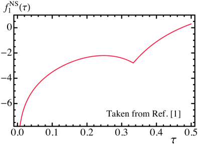
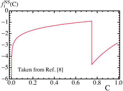
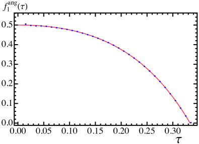
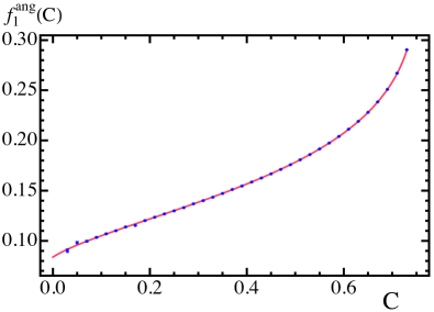
Figure 5: Averaged non-singular and angular distributions at $\mathcal{O}(\alpha_{\rm S})$. The left top panel (a) shows the thrust non-singular averaged distribution and the right top panel (b) shows the $C$-parameter non-singular averaged distribution. The left bottom panel (c) corresponds to the thrust angular distribution and the right bottom panel (d) to the $C$-parameter angular distribution. The solid line is obtained with an analytical computation, whereas blue dots with tiny error bars are the LO output of our Event2 runs. The exact definitions of $f_{1}^{\rm NS}$ and $f_{1}^{\rm ang}$ can be found in Eq. (50). The fact that the angular distributions tend to a finite value for $\tau$ or $C$ tending to zero discards singular terms, as predicted by SCET.

4 Angular Dependence to All Orders

As long as electroweak interactions between the initial and the final state are ignored, at any order (or equivalently for an arbitrary number $n$ of final-state particles) the matrix element is given by the contraction of a leptonic and a hadronic tensor. The leptonic tensor has the same form as in Eq. (6), and the hadronic tensor has the general form 

$$H^{\mu\nu} =A_{0}(q_{r}\cdot q_{s},m_{h})\,g^{\mu\nu}+\sum_{i,j=1}^{n}A_{ij}(q_{r}\cdot q_{s},m_{h})\,(q_{i}^{\mu}q_{j}^{\nu}+q_{i}^{\nu}q_{j}^{\mu})$$

$$+\sum_{i,j,k,l=1}^{n}A_{ijkl}(q_{r}\cdot q_{s},m_{h})(q_{i}^{\mu}q_{j\alpha}q_{k\beta}q_{l\gamma}\varepsilon^{\alpha\beta\gamma\nu}+q_{i}^{\nu}q_{j\alpha}q_{k\beta}q_{l\gamma}\varepsilon^{\alpha\beta\gamma\mu})$$

$$+\sum_{i,j,k=1}^{n}A_{ijk}(q_{r}\cdot q_{s},m_{h})\,q_{i\alpha}\,q_{j\beta}\,q_{k\gamma}\,\varepsilon^{\alpha\beta\gamma\mu}\,q_{i\delta}\,q_{j\rho}\,q_{k\kappa}\,\varepsilon^{\delta\rho\kappa\nu}~{},$$ (31)

where we have used the fact that the hadronic tensor is symmetric when interchanging the indices $\mu$ and $\nu$ (Imaginary parts generated by virtual corrections produce imaginary, antisymmetric tensors, which cancel upon contraction with the leptonic tensor. The symmetric part is real). When contracting leptonic and hadronic tensors one obtains a piece which is independent of the direction of the incoming electron and positron, and a piece which depends of the orientation of the hadrons with respect to the beam. We get

$$L_{\mu\nu}H^{\mu\nu} =A_{0}(q_{r}\cdot q_{s},m_{h})+\sum_{i,j=1}^{n}2\,A_{ij}(q_{r}\cdot q_{s},m_{h})[(p_{1}\cdot q_{i})(p_{2}\cdot q_{j})+(p_{2}\cdot q_{i})(p_{1}\cdot q_{j})]$$

$$+\sum_{i,j,k,l=1}^{n}A_{ijkl}(q_{r}\cdot q_{s},m_{h})[(p_{1}\cdot q_{i})\,q_{j\alpha}\,q_{k\beta}\,q_{l\gamma}\,p_{2\mu}\varepsilon^{\alpha\beta\gamma\mu}+(p_{2}\cdot q_{i})\,q_{j\alpha}\,q_{k\beta}\,q_{l\gamma}\,p_{1\mu}\varepsilon^{\alpha\beta\gamma\mu}]$$

$$+\sum_{i,j,k=1}^{n}A_{ijk}(q_{r}\cdot q_{s},m_{h})\,q_{i\alpha}\,q_{j\beta}\,q_{k\gamma}\,p_{1\mu}\,\varepsilon^{\alpha\beta\gamma\mu}q_{i\delta}\,q_{j\rho}\,q_{k\kappa}\,p_{2\nu}\,\varepsilon^{\delta\rho\kappa\nu}~{}.$$ (32)

We are interested in the dependence on the angles of the final-state particles with the incoming electron. It comes solely from scalar products of the type

$$(p_{1}\cdot q_{i})(p_{2}\cdot q_{j})+(p_{2}\cdot q_{i})(p_{1}\cdot q_{j})=\dfrac{Q^{2}}{2}\,E_{i}\,E_{j}-2\,(\vec{p}_{1}\cdot\vec{q}_{i})(\vec{p}_{1}\cdot\vec{q}_{j})~{},$$ (33)

$$q_{i\alpha}\,q_{j\beta}\,q_{k\gamma}\,p_{1\mu}\,\varepsilon^{\alpha\beta\gamma\mu}q_{i\delta}\,q_{j\rho}\,q_{k\kappa}\,p_{2\nu}\,\varepsilon^{\delta\rho\kappa\nu}=\dfrac{Q^{2}}{4}\big{[}\vec{q}_{i}\cdot(\vec{q}_{j}\times\vec{q}_{k})\big{]}^{2}$$

$$\qquad\qquad\qquad\qquad-\Big{[}\vec{p}_{1}\cdot(E_{i}\,\vec{q}_{j}\times\vec{q}_{k}+E_{j}\,\vec{q}_{k}\times\vec{q}_{i}+E_{k}\,\vec{q}_{i}\times\vec{q}_{j})\Big{]}^{2}~{},$$

$$(p_{1}\cdot q_{i})\,q_{j\alpha}\,q_{k\beta}\,q_{l\gamma}\,p_{2\mu}\,\varepsilon^{\alpha\beta\gamma\mu}+(p_{2}\cdot q_{i})\,q_{j\alpha}\,q_{k\beta}\,q_{l\gamma}\,p_{1\mu}\,\varepsilon^{\alpha\beta\gamma\mu}=\dfrac{Q^{2}}{2}\,\vec{q}_{j}\cdot(\vec{q}_{l}\times\vec{q}_{k})$$

$$\qquad\qquad\qquad\qquad-2\,(\vec{p}_{1}\cdot\vec{q}_{i})\big{[}\,\vec{p}_{1}\cdot(E_{j}\,\vec{q}_{k}\times\vec{q}_{l}+E_{k}\,\vec{q}_{l}\times\vec{q}_{j}+E_{l}\,\vec{q}_{j}\times\vec{q}_{k})\,\big{]}~{}.$$

The expression above is invariant under the transformation $\vec{p}_{1}\to-\,\vec{p}_{1}$. Plugging Eq. (33) into Eq. (4) one gets

$$L_{\mu\nu}H^{\mu\nu} =C_{0}(q_{k}\cdot q_{l},m_{h})+\sum_{i,j=1}^{n}C_{ij}(q_{r}\cdot q_{s},m_{h})\,(\vec{p}_{1}\cdot\vec{q}_{i})(\vec{p}_{1}\cdot\vec{q}_{j})$$ (34)

$$+\sum_{i,j,k}C_{ijk}(q_{r}\cdot q_{s},m_{h})\,(\vec{p}_{1}\cdot\vec{q}_{i})\,[\,\vec{p}_{1}\cdot(\vec{q}_{j}\times\vec{q}_{k})\,]$$

$$+\sum_{i,j,k,l}C_{ijkl}(q_{r}\cdot q_{s},m_{h})\,[\,\vec{p}_{1}\cdot(\vec{q}_{i}\times\vec{q}_{j})\,]\,[\,\vec{p}_{1}\cdot(\vec{q}_{k}\times\vec{q}_{l})\,]\,.$$

The next step is to integrate Eq. (34) with the phase-space of $n$ particles and a delta function that projects out $\cos\theta_{T}$.

In order to proof that the only angular structures that one can find at any order are precisely those found at LO we will make extensive use of two important properties of the thrust axis. From the definition of thrust $T$ one has

$$\Big{(}\sum_{i}|\vec{q}_{i}|\Big{)}\,T =\max_{\hat{n}}\sum_{i}|\hat{n}\cdot\vec{q}_{i}|=\max_{\hat{n}}\bigg{|}\hat{n}\cdot\Big{(}\sum_{i\in a}\vec{q}_{i}\,-\sum_{i\in b}\vec{q}_{i}\Big{)}\bigg{|}$$ (35)

$$=2\max_{\hat{n}}\bigg{|}\hat{n}\cdot\sum_{i\in a}\vec{q}_{i}\bigg{|}\equiv 2\max_{\hat{n}}\big{|}\hat{n}\cdot\vec{P}_{a}\big{|}\,.$$

Where the hemisphere $a$ contains all particles $\vec{q}_{i}$ satisfying $\hat{n}\cdot\vec{q}_{i}>0$, whereas hemisphere $b$ has particles with $\hat{n}\cdot\vec{q}_{i}<0$. In the one-to-last last equality we have used three-momentum conservation. In the last equality we have defined the total four-momentum in one hemisphere

$$P^{\mu}_{a}=\sum_{i\in a}q^{\mu}_{i}\,,\qquad P^{\mu}_{b}=\sum_{i\in b}q^{\mu}_{i}\,,$$ (36)

and of course $\vec{P}_{a}=-\,\vec{P}_{b}$. We use the notation $P_{a,b}^{2}\equiv S_{a,b}$, which are the masses of each hemisphere. The fist important property of the thrust axis is that particles can be clustered together (that is they can substituted by a pseudo-particle whose momentum is the sum of the momenta of the clustered particles) as long as they belong to the same hemisphere. The next step is to find the unitary vector $\hat{n}$ which maximizes $T$. It is obvious that this is achieved if $\hat{n}$ points in the direction of $\vec{P}_{a}$ itself

$$\hat{n}=\dfrac{\vec{P}_{a}}{|\vec{P}_{a}|}\,,\qquad T=\dfrac{2\,|\vec{P}_{a}|}{\sum_{i}|\vec{q}_{i}|}\,.$$ (37)

Hence $T$ can be thought as the length of the longest possible vector that can be formed by clustering particles together, normalized to half of the sum of the magnitudes of the final-state three-momenta.

The phase-space of $n$ particles is

$$\mathrm{d}\phi_{n}(P;\,q_{1},\ldots,q_{n}) =\Bigg{(}\prod_{i=1}^{n}\,\dfrac{\mathrm{d}^{3}\vec{q}_{i}}{2E_{i}(2\pi)^{3}}\Bigg{)}(2\pi)^{4}\,\delta^{(4)}\Big{(}P-\sum_{i=1}^{n}q_{i}\Big{)}\,,$$ (38)

$$E_{i} =\sqrt{\vec{q}_{i}^{\,2}+m_{i}^{2}}\,,$$

$$\mathrm{d}^{3}\vec{q}_{i} =\vec{q}_{i}^{\,2}\,\mathrm{d}|\vec{q}_{i}|\,\mathrm{d}\varphi_{i}\,\mathrm{d}\!\cos\theta_{i}\,.$$

Here $P$ represents the total momentum of the incoming leptons in the center-of-mass frame: $P=(Q,\,\vec{0})$. The phase-space integral can be decomposed in a series of sectors such that the $n$ particles can be clustered into two hemispheres containing $k$ and $n-k$ particles, respectively. This decomposition can be implemented by suitable theta functions which add up to one. For the case of three partons worked out in Sec. 3 these $\theta$’s read

$$\theta(x_{1}-x_{2})\,\theta(x_{1}-x_{3})\,+\,\theta(x_{2}-x_{1})\,\theta(x_{2}-x_{3})\,+\,\theta(x_{3}-x_{1})\,\theta(x_{3}-x_{2})=1\,.$$ (39)

For each one of these sectors the phase-space factorizes in the following way:

$$\!\!\!\!\!\!\mathrm{d}\phi_{n}(P;q_{1},\ldots,q_{n})=\!\int\!\dfrac{\mathrm{d}S_{a}}{2\pi}\dfrac{\mathrm{d}S_{b}}{2\pi}\,\mathrm{d}\phi_{2}(P;P_{a},P_{b})\,\mathrm{d}\phi_{k}(P_{a};q_{1},\ldots,q_{k})\,\mathrm{d}\phi_{n-k}(P_{b};q_{k+1},\ldots,q_{n})\,.$$ (40)

The projecting delta function in this sector reads

$$\delta_{T}=\delta\Bigg{(}\!\cos\theta_{T}-\dfrac{\sum_{i=1}^{k}|\vec{q}_{i}|\cos\theta_{i}}{|\sum_{i=1}^{k}\vec{q}_{i}|}\Bigg{)}.$$ (41)

In Eq. (40), the initial momentum in $\mathrm{d}\phi_{n}$ is used in the center-of-mass frame, $\vec{P}=\vec{0}$ but in $\mathrm{d}\phi_{k}$ and $\mathrm{d}\phi_{n-k}$ is not, $\vec{P}_{a,b}\neq\vec{0}$. Moreover, the azimuthal $\phi$ and polar $\theta$ angles in $\mathrm{d}\phi_{n}$ are measured with respect to the direction of the beam (that is with respect to the incoming electron), whereas for $\mathrm{d}\phi_{k}$ and $\mathrm{d}\phi_{n-k}$ they are measured with respect to $\vec{P}_{a}$. One should integrate a minimal amount of variables such that one can still later project onto any observable. We shall see that one only needs to integrate over one trivial azimuthal angular dependence to show that the pattern of Eq. (27) prevails to all orders.

Next, we integrate $\mathrm{d}^{3}\vec{P}_{b}$, $\mathrm{d}^{3}\vec{p}_{1}$ and $\mathrm{d}^{3}\vec{p}_{k+1}$ with the three corresponding spatial delta functions. This simplifies Eq. (41) to $\delta_{T}=\delta(\cos\theta_{T}-\cos\theta_{a})$ and the two-particle phase-space can be resolved completely

$$\mathrm{d}\phi_{2}(P;P_{a},P_{b})=\dfrac{1}{16\pi}\dfrac{\lambda^{\frac{1}{2}}(Q^{2},S_{a},S_{b})}{Q^{2}}\,\mathrm{d}\!\cos\theta_{a}\,,$$ (42)

where $\lambda(a,b,c)=(a+b-c)^{2}-4\,a\,b$ stands for the completely symmetric Källen function. In the matrix element Eq. (34) one has to make the replacements 

$$\vec{q}_{1}=\vec{P}_{a}-\sum_{i=2}^{k}\vec{q}_{i}\,,$$ (43)

$$\vec{q}_{k+1}=-\,\vec{P}_{a}-\sum_{i=k+2}^{n}\vec{q}_{i}\,,$$

$$\vec{p}_{1}\cdot\vec{P}_{a}=\frac{Q}{2}|\vec{P}_{a}|\cos\theta_{T}\,,$$

$$\vec{p}_{1}\cdot\vec{q}_{i}=\frac{Q}{2}|\vec{q}_{i}|\,(\sin\theta_{T}\sin\theta_{i}\cos\varphi_{i}+\cos\theta_{T}\cos\theta_{i})\,,$$

$$\vec{p}_{1}\cdot(\vec{P}_{a}\times\vec{q}_{i})=-\,\dfrac{Q}{2}|\vec{P}_{a}||\vec{q}_{i}|\sin\theta_{T}\sin\theta_{i}\sin\varphi_{i}\,,$$

$$\vec{p}_{1}\cdot(\vec{q}_{i}\times\vec{q}_{j})=\dfrac{Q}{2}|\vec{q}_{i}||\vec{q}_{j}|[\sin\theta_{T}(\sin\theta_{i}\cos\theta_{j}\sin\varphi_{i}-\sin\theta_{j}\cos\theta_{i}\sin\varphi_{j})$$

$$\qquad\qquad\qquad+\cos\theta_{T}\sin\theta_{i}\sin\theta_{j}\sin\varphi_{ji}]\,,$$

with $\varphi_{ji}=\varphi_{j}-\varphi_{i}$. Here we have taken the beam axis to lie on the $x-z$ plane, hence $\varphi_{T}=0$. An important observation is that $\sin\theta_{T}$ is always multiplied by a single power of $\cos\varphi_{i}$ or $\sin\varphi_{i}$. Now Eq. (34) becomes

$$L_{\mu\nu}H^{\mu\nu}=D^{(0)}(q_{k}\cdot q_{l},m_{h},\cos\varphi_{i},\cos\theta_{j})+\cos^{2}\theta_{T}\,D^{(1)}(q_{k}\cdot q_{l},m_{h},\cos\varphi_{s},\sin\varphi_{t},\cos\theta_{m})$$

$$+\sin\theta_{T}\cos\theta_{T}\Bigg{[}\sum_{i}\cos\varphi_{i}\,D^{(2)}_{i}(q_{k}\cdot q_{l},m_{h},\cos\theta_{m})+\sum_{i}\sin\varphi_{i}\,D^{(3)}_{i}(q_{k}\cdot q_{l},m_{h},\cos\theta_{m})$$

$$+\sum_{ijk}\cos\varphi_{i}\sin\varphi_{jk}\,D^{(4)}_{i}(q_{k}\cdot q_{l},m_{h},\cos\theta_{m})+\sum_{ijk}\sin\varphi_{i}\sin\varphi_{jk}\,D^{(5)}_{i}(q_{k}\cdot q_{l},m_{h},\cos\theta_{m})\Bigg{]}\,,$$ (44)

where we have substituted $\sin^{2}\theta_{T}=1-\cos^{2}\theta_{T}$. Additionally, in $\mathrm{d}\phi_{k}$ and $\mathrm{d}\phi_{n-k}$ one has to make the following replacements:

$$\vec{q}_{1}^{\,2} =\vec{P}_{a}^{\,2}-2\,|\vec{P}_{a}|\sum_{i=2}^{k}|\vec{q}_{i}|\cos\theta_{i}+\sum_{i,j=2}^{k}|\vec{q}_{i}||\vec{q}_{j}|(\sin\theta_{i}\sin\theta_{j}\cos\varphi_{ij}+\cos\theta_{i}\cos\theta_{j})\,,$$ (45)

$$\vec{q}_{k+1}^{\,2} =\vec{P}_{a}^{\,2}+2\,|\vec{P}_{a}|\sum_{i=k+2}^{n}|\vec{q}_{i}|\cos\theta_{i}+\sum_{i,j=k+1}^{n}|\vec{q}_{i}||\vec{q}_{j}|(\sin\theta_{i}\sin\theta_{j}\cos\varphi_{ij}+\cos\theta_{i}\cos\theta_{j})\,.$$

The important observation is that the dependence on the azimuthal angles is always through the difference of two angles. Hence one can make the following change of variables: $\varphi_{i}\to\varphi_{i}+\varphi_{k}$ and completely eliminate the dependence on $\varphi_{k}$ from the phase-space, which can then trivially be integrated. One should choose $\varphi_{k}$ term by term in Eq. (4) such that the term proportional to $\sin\theta_{T}\cos\theta_{T}$ vanishes upon azimuthal angular integration. This works trivially for the terms with a single power of $\sin\varphi_{i}$ or $\cos\varphi_{i}$ by taking $\varphi_{k}=\varphi_{i}$, but also with terms such as $\cos\varphi_{i}\sin\varphi_{jl}$ or $\sin\varphi_{i}\sin\varphi_{jl}$. In the latter case, if $i\neq j\neq l$ one can make $\varphi_{k}=\varphi_{i}$, if $j=l$ then the term is automatically zero, and if $i=j$ then one can choose $\varphi_{k}=\varphi_{l}$. It is important to stress that no event-shape variable can depend on the overall azimuthal angle around the thrust axis, and hence this integral can always be performed completely. In a way we are averaging the event shape distribution with respect to the azimuthal direction around the thrust axis. Similarly, the phase space decomposition does not depend on a global azimuthal orientation either. One would get sensitivity to it only if the beam is polarized. This global azimuthal angle is represented in Fig. 1 as $\varphi_{T}$.

This procedure can be repeated sector by sector in exactly the same way. The outcome is that only $\theta_{T}$-independent structures and terms proportional to $\cos^{2}\theta_{T}$ can arise. These can be conveniently recast into $F_{0}(\cos\theta_{T})=3/8\,(1+\cos^{2}\theta_{T})$ and $F_{1}(\cos\theta_{T})=1-3\cos^{2}\theta_{T}$. One can afterwards project onto any event-shape $e$ by the appropriate delta function, and in full generality the result can be expressed as

$$\dfrac{1}{\sigma_{0}}\dfrac{\mathrm{d}\sigma}{\mathrm{d}\!\cos\theta_{T}\,\mathrm{d}e} =\dfrac{1}{\sigma_{0}}\dfrac{\mathrm{d}\sigma}{\mathrm{d}e}\,F_{0}(\cos\theta_{T})+\dfrac{1}{\sigma_{0}}\dfrac{\mathrm{d}\sigma_{\rm ang}}{\mathrm{d}e}\,F_{1}(\cos\theta_{T})\,,$$ (46)

$$\dfrac{1}{\sigma_{0}}\dfrac{\mathrm{d}\sigma}{\mathrm{d}e} =\int_{-1}^{1}\mathrm{d}\!\cos\theta_{T}\,\dfrac{1}{\sigma_{0}}\dfrac{\mathrm{d}\sigma}{\mathrm{d}\!\cos\theta_{T}\,\mathrm{d}e}\,,$$

$$\dfrac{1}{\sigma_{0}}\dfrac{\mathrm{d}\sigma_{\rm ang}}{\mathrm{d}e} =\dfrac{3}{8}\int_{-1}^{1}\mathrm{d}\!\cos\theta_{T}\,(2-5\cos^{2}\theta_{T})\,\dfrac{1}{\sigma_{0}}\dfrac{\mathrm{d}\sigma}{\mathrm{d}\!\cos\theta_{T}\,\mathrm{d}e}\,.$$

We will refer to the cross-section multiplying $F_{0}$ as the “averaged distribution”, and will refer to the cross-section multiplying $F_{1}$ as the “angular distribution”. As a final comment we would like to emphasize that the proof is valid for partons (massless or massive) as well as for hadrons, and hence the general structure of Eq. (46) “survives” hadronization. In Refs. Lampe:1992au ; Hagiwara:2010cd ; Abbiendi:1998at the oriented distributions are written in terms of transverse ($\sigma_{T}$) and longitudinal ($\sigma_{L}$) distributions. They are related to our notation in a simple manner: $\sigma=\sigma_{T}+\sigma_{L}$ and $\sigma_{\rm ang}=3/8\,\sigma_{L}$.

In Ref. Lampe:1992au it is shown that for three-parton processes the only two possible structures are the same as in Eq. (46). For processes with higher multiplicity the longitudinal cross section is defined as the contraction of the hadronic tensor with the two longitudinal polarization vectors of an intermediate massive vector boson, but no proof is given that this contraction renders the angular structure predicted in Eq. (46). Similarly Ref. Abbiendi:1998at claims that Eq. (46) is the most general result, without proof or quote. Finally, in Ref. Hagiwara:2010cd an alternative proof for Eq. (46) is presented. The proof relies on current conservation (hence it would not apply to production of heavy quarks by an axial current, and hence is not as general as ours). Moreover, their demonstration assumes a particular Lorentz structure for the thrust-oriented hadronic tensor in terms of four-vectors constructed out of the thrust axis direction. This structure is presented without a rigorous proof, and it would certainly not hold for some other choices of the oriented axis. In a sense, our demonstration could be used to proof their proposed hadronic tensor structure.

We finish this section with a discussion of the case in which parity-violating terms can arise. The generalization is straightforward and it only requires to assign a direction to the thrust axis . We will assume that the thrust axis points into he $\vec{P}_{a}$ direction. Parity violating terms and virtual effects induce antisymmetric lepton and hadron tensors, which are purely imaginary. In the lepton case one has antisymmetric terms though axial contributions

$$L_{A}^{\mu\nu}\propto i\,p_{1\alpha}\,p_{2\beta}\,\varepsilon^{\alpha\beta\mu\nu}\,.$$ (47)

Similarly the antisymmetric part of the hadronic tensor would look like

$$H_{A}^{\mu\nu}=\sum_{i,j}\bigg{[}A_{ij}\,q_{i\alpha}\,q_{j\beta}\,\varepsilon^{\alpha\beta\mu\nu}+B_{ij}(q_{i}^{\mu}\,q_{j}^{\nu}-q_{i}^{\nu}\,q_{j}^{\mu})\bigg{]}\,,$$ (48)

when contracting the antisymmetric parts of the leptonic and hadronic tensors one is left with two kind of terms:

$$L_{\mu\nu,A}\,H_{A}^{\mu\nu}\propto Q\sum_{i,j}\bigg{[}A_{ij}\,\vec{p}_{1}\cdot(E_{j}\,\vec{q}_{i}-E_{i}\,\vec{q}_{j})+2\,B_{ij}\,\vec{p}_{1}\cdot(\vec{q}_{i}\times\vec{q}_{j})\bigg{]}\,.$$ (49)

Following the same steps as for the parity-conserving terms one arrives to the conclusion that only terms linear in $\cos\theta_{T}$ can arise (that is there are no terms proportional to $\sin\theta_{T}$, since they cancel upon azimuthal angle integration). These terms contain singular and non-singular terms, and the former can be treated in SCET in the same way as the averaged distribution.

5 NLO Distribution

In this section we present results for the non-singular and angular cross-sections for thrust, $C$-parameter, Heavy-Jet Mass and the sum of Hemisphere Masses . To that end we run the FORTRAN program Event2 Catani:1996jh ; Catani:1996vz with $6\times 10^{11}$ events.

The event-shape cross-section can be expanded in powers of $\alpha_{\rm S}$. Since we carry out resummation for the most singular terms of the averaged distribution, we do not use the fixed-order counting for them, instead we use resummed counting (LL, NLL, etc …). For the non-singular averaged distribution and the angular distribution we use the following expansion :

$$\dfrac{1}{\sigma_{0}}\dfrac{\mathrm{d}\sigma_{\rm NS}}{\mathrm{d}e} =\dfrac{\alpha_{\rm S}(Q)}{\pi}f_{1}^{\rm NS}(e)+\bigg{(}\dfrac{\alpha_{\rm S}(Q)}{\pi}\bigg{)}^{2}f_{2}^{\rm NS}(e)+\bigg{(}\dfrac{\alpha_{\rm S}(Q)}{\pi}\bigg{)}^{3}f_{3}^{\rm NS}(e)+\ldots$$ (50)

$$\dfrac{1}{\sigma_{0}}\dfrac{\mathrm{d}\sigma_{\rm ang}}{\mathrm{d}e} =\dfrac{\alpha_{\rm S}(Q)}{\pi}f_{1}^{\rm ang}(e)+\bigg{(}\dfrac{\alpha_{\rm S}(Q)}{\pi}\bigg{)}^{2}f_{2}^{\rm ang}(e)+\bigg{(}\dfrac{\alpha_{\rm S}(Q)}{\pi}\bigg{)}^{3}f_{3}^{\rm ang}(e)+\ldots$$

Similarly we also expand the averaged and angular total cross-sections as

$$R_{\rm had} =1+\dfrac{\alpha_{\rm S}(Q)}{\pi}R_{1}+\bigg{(}\dfrac{\alpha_{\rm S}(Q)}{\pi}\bigg{)}^{2}R_{2}+\bigg{(}\dfrac{\alpha_{\rm S}(Q)}{\pi}\bigg{)}^{3}R_{3}+\ldots$$ (51)

$$R_{\rm ang} =\dfrac{\alpha_{\rm S}(Q)}{\pi}R_{1}^{\rm ang}+\bigg{(}\dfrac{\alpha_{\rm S}(Q)}{\pi}\bigg{)}^{2}R_{2}^{\rm ang}+\bigg{(}\dfrac{\alpha_{\rm S}(Q)}{\pi}\bigg{)}^{3}R_{3}^{\rm ang}+\ldots$$

Finally one can define the integrated or cumulant cross-section

$$\Sigma_{\rm ang}(e_{c}) =\dfrac{1}{\sigma_{0}}\int_{0}^{e_{c}}\mathrm{d}e\,\dfrac{\mathrm{d}\sigma_{\rm ang}}{\mathrm{d}e}\,,$$ (52)

$$=\dfrac{\alpha_{\rm S}(Q)}{\pi}\,\Sigma_{1}^{\rm ang}(e_{c})+\bigg{(}\dfrac{\alpha_{\rm S}(Q)}{\pi}\bigg{)}^{2}\Sigma_{2}^{\rm ang}(e_{c})+\bigg{(}\dfrac{\alpha_{\rm S}(Q)}{\pi}\bigg{)}^{3}\Sigma_{3}^{\rm ang}(e_{c})+\ldots$$

At ${\mathcal{O}}(\alpha_{\rm S})$ we find the following analytic result for thrust

$$\Sigma_{1}^{\rm ang}(\tau)=-\,\dfrac{3}{8}\,C_{F}\Bigg{[}\dfrac{\tau\,(7-3\tau)}{1-\tau}+8\,\log(1-\tau)\Bigg{]}\,.$$ (53)

The expressions for arbitrary $\mu$ can be trivially obtained by expanding out $\alpha_{\rm S}(Q)$ in terms of $\alpha_{\rm S}(\mu)$ and $\log(\mu/Q)$. The best strategy to obtain the two angular pieces is to directly project them out of the Event2 runs, using the second and third lines of Eq. (46). The corresponding integrals can be performed event by event (that is, one does not need to make a two-dimensional grid in the event-shape and $\cos\theta_{T}$ and integrate later). The cross-section of each event is simply weighted by either $1=P_{0}(\cos\theta_{T}^{i})$ or $3/8\,(2-5\cos^{2}\theta^{i}_{T})=1/8-5/4\,P_{2}(\cos\theta_{T}^{i})$ to project out the averaged and angular pieces respectively. $\theta^{i}_{T}$ is the angle formed by the incoming electron and the thrust axis for the particular event configuration. Since the projecting functions can be expressed in terms of linear combinations of Legendre polynomials of order less than $3$, any hypothetical additional angular structure expressed in terms of higher-order polynomial would be averaged out. Finally events are clustered in histograms according to event-shape values.

As a cross check of the validity of Eq. (46) we try to project out additional angular structures. So we assume that there exist angular terms proportional to higher-order Legendre polynomials. Since we only care about parity-conserving distributions only polynomials $P_{n}$ with even $n$ can appear. We have projected out terms proportional to $P_{4}(\cos\theta_{T})$ and $P_{6}(\cos\theta_{T})$, which are obtained by integrating with $9/2\,P_{4}(\cos\theta_{T})$ and $13/2\,P_{6}(\cos\theta_{T})$, respectively. It is important to note that since $F_{2}(\cos\theta_{T})=1/2+1/8\,P_{2}(\cos\theta_{T})$ and $F_{1}(\cos\theta_{T})=-\,2\,P_{2}(\cos\theta_{T})$ these two additional projections are not affected by the $F_{0}$ and $F_{1}$ terms. We found, as expected, that the projected out terms are compatible with zero for all event-shapes.

In Fig. 6 we show the extracted non-singular term for the sum of Hemisphere Masses. We directly compute the sum of all color structures, for the phenomenologically relevant case of five light flavors. As it is well known, at the partonic level (that is for massless particles) thrust and the sum of Hemisphere Masses are identical in the dijet limit [ see Eq. (5) ], and hence their singular distributions coincide to all orders in perturbation theory. Non-singular terms are however different. The procedure to extract the non-singular terms is identical to that followed in Abbate:2010xh : we use a fit function below $\rho_{S}=0.1$, which is fitted to logarithmically binned Event2 data. Above $\rho_{S}=0.1$, where errors are negligibly small, we use an interpolation function over linearly binned Event2 data. For completeness we also show in Fig. 6 the NLO non-singular distributions for thrust, Heavy-Jet Mass and $C$-parameter.

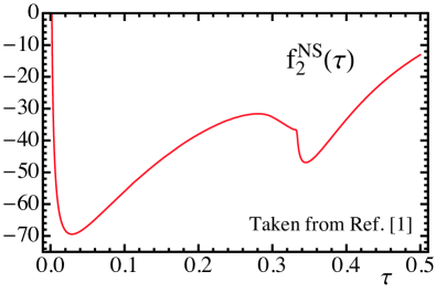
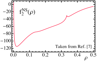
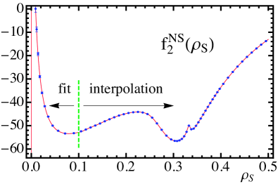
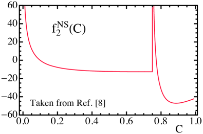
Figure 6: Non-singular distributions at $\mathcal{O}(\alpha_{\rm S}^{2})$ for (a) thrust, (b) Heavy-Jet Mass, (c) the sum of Hemisphere Masses and (d) $C$-parameter. For the sum of Hemisphere Masses, the blue dots correspond to Event2 output, linearly binned to the right of the green dashed line, and logarithmically binned to the left. The red line corresponds to the function that we implement in our numerical code. To the right of the dashed line we use an interpolating function, whereas to the left we use a fit function. The error band corresponding to the fit function is too small to be visible in this plot. For the other event shapes the non-singular function was determined in other publications.

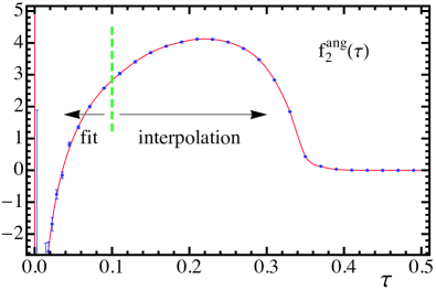
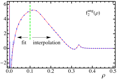
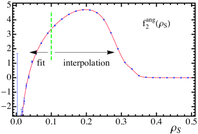
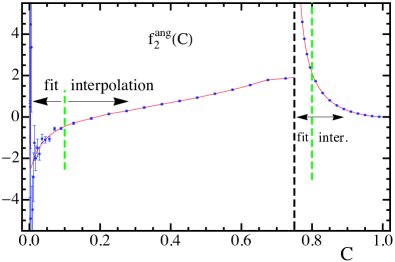
Figure 7: Angular distributions at $\mathcal{O}(\alpha_{\rm S}^{2})$. All the color structures with $n_{f}=5$ are summed. The blue dots show the Event2 output, linearly binned to the right of the green dashed line, and logarithmically binned to the left. The red line corresponds to the determined function. To the right of the dashed line we use an interpolating function, whereas to the right we use a fit function. The error band corresponding to the fit function is too small to be visible in this plot. The panels correspond to thrust (a); Heavy-Jet Mass (b), the sum of the Hemisphere Masses (c) and $C$-parameter (d). In panel (d), the black dashed line shows the position of the “shoulder”, which corresponds to the four-particle threshold. We use a fit function and logarithmically binned Event2 output between the green and black dashed lines, and an interpolation with linearly binned Event2 output above the second green line.

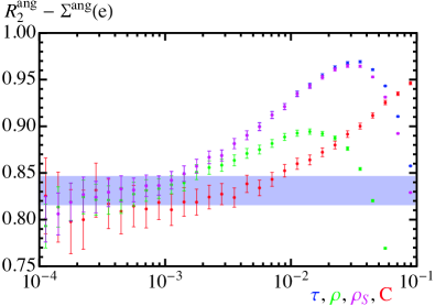
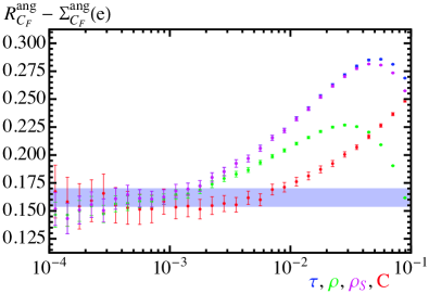
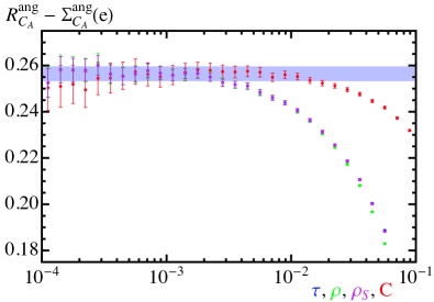
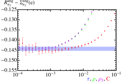
Figure 8: Computation of the angular piece for oriented total cross-section [ see Eqs. (28), (51) and (54) ] from Event2 output. The cross-section is obtained by extrapolating to zero, which is simpler with logarithmic binning. The extrapolation is shown as a blue band. In each plot we show various event-shape variables $e$: thrust in blue, $C$-parameter in red, Heavy-Jet Mass in green and the sum of Hemisphere Masses in magenta. $\Sigma_{2}$ is the cumulant cross section, and it is defined in Eq. (52). In all cases, all event-shapes converge to the same value for small values of the shape variable. In panel (a) the sum of the various color pieces for $n_{f}=5$ is shown; (b) shows the $C_{F}^{2}$ piece, (c) the $C_{F}C_{A}$ piece and (d) the $C_{F}T_{f}n_{f}$ term.

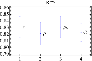
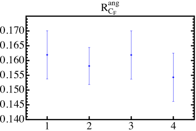
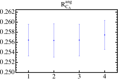
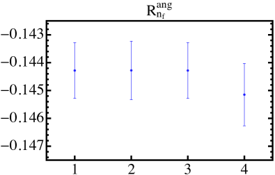
Figure 9: Comparison of the determination of the angular piece for oriented total cross-section. On the horizontal axis $1$ corresponds to Thrust, $2$ to Heavy-Jet Mass, $3$ to the sum of the Hemisphere Masses, and $4$ to $C$-parameter. In panel (a) the sum of the various color pieces for $n_{f}=5$ is shown; (b) shows the $C_{F}^{2}$ piece, (c) the $C_{F}C_{A}$ piece and (d) the $C_{F}T_{f}n_{f}$ term.

In Fig. 7 we show the angular fixed-order distribution at $\mathcal{O}(\alpha_{\rm S}^{2})$ for thrust (a), Heavy-Jet Mass (b), the sum of the Hemisphere Masses (c) and $C$-parameter (d), as extracted from the Event2 program. We have summed all color structures for $n_{f}=5$. Since the angular piece is numerically much smaller than the averaged one, the relative errors are significantly larger. The strategy that we follow is the same as for the non-singular terms of $\rho_{S}$, with a slight modification: the fit function coefficients have an explicit dependence on the value of $R_{2}^{\rm ang}$, which is known only numerically (see below). In this way, if we vary the value of $R_{2}^{\rm ang}$ within errors, the fit function is varied accordingly, in such a way that the total integral is always $R_{2}^{\rm ang}$, and the angular cross-section is exactly normalized to one. The determination of the $C$-parameter deserves further explanation. Since the ${\mathcal{O}}(\alpha_{\rm S})$ fixed-order distribution does not fall off to zero in the completely symmetric configuration in which the three partons have the same energy (that is for $C=3/4$), the cross-sections has a log-integrable singularity at ${\mathcal{O}}(\alpha_{\rm S}^{2})$, located precisely at $C=3/4$. This happens both for the averaged and the angular distributions  . This behavior is known as the shoulder, and a detailed explanation on its physical origin and how to resum the corresponding logs can be found in Ref. Catani:1997xc . We made a dedicated Event2 run for the region above the shoulder, logarithmically binned around $C=3/4$, that is we made histograms in the variable $\log_{10}(C-3/4)$. We use a fit function for the region $3/4>C>0.8$ using the log-binned output, and a fit function on for $C>0.8$ on linearly binned Event2 data.

The last piece of information that one needs to extract from Event2 is the two-loop averaged total cross-section. Unfortunately one cannot simply sum all of the randomly generated events, since Event2 discards events in which partons are too close to each other, which means that the extreme dijet region is not correctly described. This is clearly visible in the histograms since for very small values of the event-shape errors are unnaturally large and central values stop following a natural trend. What one has to do instead is to sum up all events which produce values of a given event-shape $e$ bigger that a small value $e_{\rm min}$, and then extrapolate to $e_{\rm min}\to 0$. To do that we can use any event-shape. The simplest way is using a linearly binned histogram, and linearly (or using a higher-degree polynomial) extrapolate to zero using the last few points. We discard this procedure because the extrapolation is affected by logarithms [ near zero the sum of bins behaves as $R_{2}^{\rm ang}+e\,\sum_{i}\log^{i}(e)$ ]. A better strategy is to use a logarithmically binned histogram. In this case when approaching the dijet limit, the sum of histograms becomes exponentially close to $R_{2}^{\rm ang}$. It is very simple to realize that this regimes has been reached, since graphically the distribution becomes very flat (see Fig. 8). This method was first applied in Ref. Hoang:2008fs . To be more definite, we proceed as follows: first we select a set of points that a) have central values which not show an increasing or decreasing trend (they are flat within statistical fluctuations), this cuts off points with too big value of the event-shape; and b) are not yet affected by cutoff effects, which limits the points with very small value of the event-shape. Given these points, we determine the central value by averaging the central values (we do not make a weighted average since errors are highly correlated). We determine a “statistical” uncertainty by averaging the uncertainties of all the points. We assign a systematic uncertainty by taking half of the maximum difference of central values. We have used $\tau$, $\rho$, $\rho_{S}$ and $C$ to determine $R_{2}^{\rm ang}$ and we find very good agreement in each color structure, as can be seen in Fig. 9.

Defining

$$R_{2}^{\rm ang}=C_{F}^{2}\,R^{\rm ang}_{C_{\!F}}+C_{F}C_{A}R^{\rm ang}_{C_{\!A}}+C_{F}T_{F}\,n_{f}R^{\rm ang}_{n_{\!f}}\,,$$ (54)

we find

$$R_{2}^{\rm ang} \;= 0.831 \;\pm 0.014 \;\pm 0.006\,,$$ (55)

$$R^{\rm ang}_{C_{\!F}} \;= 0.162 \;\pm 0.008 \;\pm 0.002\,,$$

$$R^{\rm ang}_{C_{\!A}} \;= 0.256 \;\pm 0.029 \;\pm 0.001\,,$$

$$R^{\rm ang}_{n_{\!f}} \;= \,-\,0.1443 \;\pm \;0.0008 \;\pm \;0.0006\,,$$

where the first uncertainty is statistic and the second one is systematic. Our results do not agree with those computed in Ref. Lampe:1992au . We find a much bigger correction than they do, and additionally we find an opposite sign for $R^{\rm ang}_{C_{\!F}}$. We will make additional checks of our determination in future work.

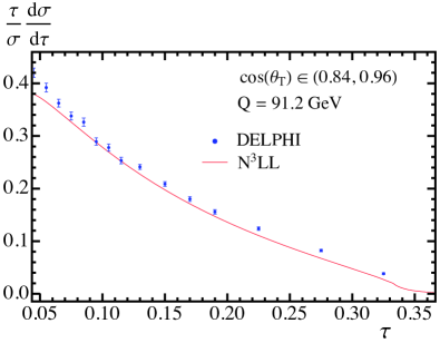
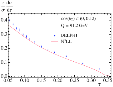
Figure 10: Comparison of our theoretical predictions (red line) with DELPHI data (blue dots) for thrust. Our theoretical prediction contains resummation of singular logs at N³LL and fixed-order matrix elements at $\mathcal{O}(\alpha_{s}^{3})$ and $\mathcal{O}(\alpha_{s}^{2})$ for the total and angular distributions, respectively. No power corrections have been included, which could explain the slight disagreement with data. We use the world average value for $\alpha_{s}(m_{Z})$. We compare to the two bins in $\cos\theta_{T}$ for which the difference between the averaged and oriented distributions is maximal. In panel (a) the oriented distribution is higher than the averaged, whereas in panel (b) the opposite occurs.

In Fig. 10 we compare our theoretical predictions with DELPHI data. We compare the differential thrust distribution for two bins in $\cos\theta_{T}$. We choose these two bins since they have the largest deviation from the averaged cross section in the positive and negative directions. Our theoretical prediction is purely perturbative, and includes resummation of singular logs at N³LL and fixed-order matrix elements up to three loops.

6 Conclusions

We have performed a first theoretical analysis of oriented event-shape observables, which are double differential distributions in the event-shape variable and in the polar angle of the thrust axis with respect to the electron–positron beam, in the context of SCET. The event-shape variables analyzed were thrust, Heavy-Jet Mass, the sum of the Hemisphere Masses and $C$-parameter. We have proven that perturbation theory predicts that the angular dependence of the oriented event-shapes is parameterized in terms of only two angular structures, $F_{0}=3/8\,(1+\cos^{2}\theta_{T})$ and $F_{1}=(1-3\,\cos^{2}\theta_{T})$. The most singular contributions, as predicted by SCET, inherit the angular dependence of the lowest order process $e^{+}e^{-}\to q\bar{q}$, and therefore can arise exclusively in the term which is proportional to $F_{0}$. This general behavior is extensible to recoil-sensitive variables such as Jet Broadening because only the hard function is sensitive to the orientation of the thrust axis, and also from the partonic to the hadron level.

We have extracted from fixed-order calculations the non-singular contributions to the angular averaged cross-section, which is proportional to $F_{0}$, and the new angular contribution of the $F_{1}$ term, at $\mathcal{O}(\alpha_{\rm S})$ analytically and at $\mathcal{O}(\alpha_{\rm S}^{2})$ with the program Event2. These are all the ingredients necessary to perform the determination of the strong coupling $\alpha_{\rm S}$ from oriented event-shapes with resummed theoretical predictions at N³LL and ${\cal O}(\alpha_{\rm S}^{2})$ accuracy.

The validity of the proof in Sec. 4 can be extended to other axes other than the thrust one. In principle any axis which is defined as the sum of the 3-momenta of particles is equally valid, as this would allow to factor the phase space in a way analogous to Eq. (40). For instance, the momentum of the hardest particle, or the momentum of the hardest jet, as long as the momenta of the jet is the sum of the momenta of some of the particles it contains, are valid axes.

If LEP data are preserved Holzner:2009ew ; Akopov:2012bm at the particle level it could be reanalyzed to produce very accurate oriented-event shape distributions at energies other than the $Z$-pole. Actually it would be possible to directly determine the averaged and angular distribution using the projection procedure sketched in Eq. (46). These results would be useful also for the measurement of $\alpha_{\rm S}$ at higher energies at a future Linear Collider.

References

- (1) R. Abbate, M. Fickinger, A. H. Hoang, V. Mateu, and I. W. Stewart, Thrust at N3LL with Power Corrections and a Precision Global Fit for , Phys. Rev. D83 (2011) 074021, [arXiv:1006.3080].
- (2) T. Gehrmann, G. Luisoni, and P. F. Monni, Power corrections in the dispersive model for a determination of the strong coupling constant from the thrust distribution, arXiv:1210.6945.
- (3) T. Gehrmann, M. Jaquier, and G. Luisoni, Hadronization effects in event shape moments, Eur. Phys. J. C67 (2010) 57–72, [arXiv:0911.2422].
- (4) R. Abbate, M. Fickinger, A. H. Hoang, V. Mateu, and I. W. Stewart, Precision Thrust Cumulant Moments at LL, Phys.Rev. D86 (2012) 094002, [arXiv:1204.5746].
- (5) S. Bethke, World Summary of alphas (2011), Nucl. Phys. B Proc. Supp. (to appear) (2012).
- (6) S. Bethke, A. H. Hoang, S. Kluth, J. Schieck, I. W. Stewart, et al., Workshop on Precision Measurements of , arXiv:1110.0016.
- (7) A. H. Hoang, V. Mateu, M. Schwartz, and I. W. Stewart, Heavy Jet Mass Predictions at N3LL with Power Corrections, Work in progress (2013).
- (8) D. W. Kolodrubetz, A. H. Hoang, V. Mateu, and I. W. Stewart, C-parameter distribution at N3LL and a determination of , Work in progress (2013).
- (9) DELPHI Collaboration, P. Abreu et al., Consistent measurements of from precise oriented event shape distributions, Eur. Phys. J. C14 (2000) 557–584, [hep-ex/0002026].
- (10) S. Catani and M. H. Seymour, The Dipole Formalism for the Calculation of QCD Jet Cross Sections at Next-to-Leading Order, Phys. Lett. B378 (1996) 287–301, [hep-ph/9602277].
- (11) S. Catani and M. H. Seymour, A general algorithm for calculating jet cross sections in NLO QCD, Nucl. Phys. B485 (1997) 291–419, [hep-ph/9605323].
- (12) G. Rodrigo, A. Santamaria, and M. S. Bilenky, Do the quark masses run? Extracting m-bar(b) (m(z)) from LEP data, Phys.Rev.Lett. 79 (1997) 193–196, [hep-ph/9703358].
- (13) OPAL Collaboration Collaboration, G. Abbiendi et al., Measurement of the longitudinal cross-section using the direction of the thrust axis in hadronic events at LEP, Phys.Lett. B440 (1998) 393–402, [hep-ex/9808035].
- (14) A. Gehrmann-De Ridder, T. Gehrmann, E. W. N. Glover, and G. Heinrich, Second-order QCD corrections to the thrust distribution, Phys. Rev. Lett. 99 (2007) 132002, [arXiv:0707.1285].
- (15) A. Gehrmann-De Ridder, T. Gehrmann, E. W. N. Glover, and G. Heinrich, NNLO corrections to event shapes in annihilation, JHEP 12 (2007) 094, [arXiv:0711.4711].
- (16) S. Weinzierl, NNLO corrections to 3-jet observables in electron-positron annihilation, Phys. Rev. Lett. 101 (2008) 162001, [arXiv:0807.3241].
- (17) S. Weinzierl, Event shapes and jet rates in electron-positron annihilation at NNLO, JHEP 06 (2009) 041, [arXiv:0904.1077].
- (18) B. Lampe, On the longitudinal cross-section for Z hadrons, Phys.Lett. B301 (1993) 435–439.
- (19) K. Hagiwara and G. Kirilin, Angular distribution of thrust axis with power-suppressed contribution in annihilation, JHEP 1010 (2010) 093, [arXiv:1006.5330].
- (20) E. Farhi, A QCD Test for Jets, Phys. Rev. Lett. 39 (1977) 1587–1588.
- (21) I. W. Stewart, F. J. Tackmann, and W. J. Waalewijn, N-Jettiness: An Inclusive Event Shape to Veto Jets, Phys.Rev.Lett. 105 (2010) 092002, [arXiv:1004.2489].
- (22) V. Mateu, I. W. Stewart, and J. Thaler, Power Corrections to Event Shapes with Mass-Dependent Operators, Phys.Rev. D87 (2013) 014025, [arXiv:1209.3781].
- (23) G. Parisi, Super Inclusive Cross-Sections, Phys.Lett. B74 (1978) 65.
- (24) J. F. Donoghue, F. Low, and S.-Y. Pi, Tensor Analysis of Hadronic Jets in Quantum Chromodynamics, Phys.Rev. D20 (1979) 2759.
- (25) L. Clavelli, Jet Invariant Mass in Quantum Chromodynamics, Phys.Lett. B85 (1979) 111.
- (26) T. Chandramohan and L. Clavelli, Consequences of Second Order QCD for Jet Structure in Annihilation, Nucl.Phys. B184 (1981) 365.
- (27) L. Clavelli and D. Wyler, Kinematica Bounds on Jet Variables and the Heavy Jet Mass Distribution, Phys.Lett. B103 (1981) 383.
- (28) C. W. Bauer, S. Fleming, and M. E. Luke, Summing Sudakov logarithms in in effective field theory, Phys. Rev. D 63 (2001) 014006, [hep-ph/0005275].
- (29) C. W. Bauer, S. Fleming, D. Pirjol, and I. W. Stewart, An effective field theory for collinear and soft gluons: Heavy to light decays, Phys. Rev. D 63 (2001) 114020, [hep-ph/0011336].
- (30) C. W. Bauer and I. W. Stewart, Invariant operators in collinear effective theory, Phys. Lett. B 516 (2001) 134–142, [hep-ph/0107001].
- (31) C. W. Bauer, D. Pirjol, and I. W. Stewart, Soft-Collinear Factorization in Effective Field Theory, Phys. Rev. D65 (2002) 054022, [hep-ph/0109045].
- (32) C. W. Bauer, S. Fleming, D. Pirjol, I. Z. Rothstein, and I. W. Stewart, Hard scattering factorization from effective field theory, Phys. Rev. D 66 (2002) 014017, [hep-ph/0202088].
- (33) T. Becher and M. D. Schwartz, A Precise determination of from LEP thrust data using effective field theory, JHEP 07 (2008) 034, [arXiv:0803.0342].
- (34) Y.-T. Chien and M. D. Schwartz, Resummation of heavy jet mass and comparison to LEP data, JHEP 08 (2010) 058, [arXiv:1005.1644].
- (35) P. E. Rakow and B. Webber, Transverse Momentum Moments of Hadron Distributions in QCD Jets, Nucl.Phys. B191 (1981) 63.
- (36) T. Becher, G. Bell, and M. Neubert, Factorization and Resummation for Jet Broadening, Phys.Lett. B704 (2011) 276–283, [arXiv:1104.4108].
- (37) T. Becher and G. Bell, NNLL Resummation for Jet Broadening, JHEP 1211 (2012) 126, [arXiv:1210.0580].
- (38) C. F. Berger, T. Kúcs, and G. Sterman, Event shape / energy flow correlations, Phys. Rev. D 68 (2003) 014012, [hep-ph/0303051].
- (39) A. Hornig, C. Lee, and G. Ovanesyan, Effective Predictions of Event Shapes: Factorized, Resummed, and Gapped Angularity Distributions, JHEP 05 (2009) 122, [arXiv:0901.3780].
- (40) S. Catani, L. Trentadue, G. Turnock, and B. R. Webber, Resummation of large logarithms in event shape distributions, Nucl. Phys. B407 (1993) 3–42.
- (41) S. Catani and B. Webber, Resummed C parameter distribution in annihilation, Phys.Lett. B427 (1998) 377–384, [hep-ph/9801350].
- (42) S. Catani, G. Turnock, and B. Webber, Jet broadening measures in annihilation, Phys.Lett. B295 (1992) 269–276.
- (43) Y. L. Dokshitzer, A. Lucenti, G. Marchesini, and G. Salam, On the QCD analysis of jet broadening, JHEP 9801 (1998) 011, [hep-ph/9801324].
- (44) A. Banfi, G. P. Salam, and G. Zanderighi, Generalized resummation of QCD final state observables, Phys.Lett. B584 (2004) 298–305, [hep-ph/0304148].
- (45) A. Banfi, G. P. Salam, and G. Zanderighi, Principles of general final-state resummation and automated implementation, JHEP 0503 (2005) 073, [hep-ph/0407286].
- (46) D. de Florian and M. Grazzini, The back-to-back region in energy energy correlation, Nucl. Phys. B704 (2005) 387–403, [hep-ph/0407241].
- (47) C. W. Bauer, A. V. Manohar, and M. B. Wise, Enhanced nonperturbative effects in jet distributions, Phys. Rev. Lett. 91 (2003) 122001, [hep-ph/0212255].
- (48) C. W. Bauer, C. Lee, A. V. Manohar, and M. B. Wise, Enhanced nonperturbative effects in Z decays to hadrons, Phys. Rev. D 70 (2004) 034014, [hep-ph/0309278].
- (49) G. P. Korchemsky, Shape functions and power corrections to the event shapes, hep-ph/9806537.
- (50) G. P. Korchemsky and G. Sterman, Power corrections to event shapes and factorization, Nucl. Phys. B555 (1999) 335–351, [hep-ph/9902341].
- (51) G. P. Korchemsky and S. Tafat, On power corrections to the event shape distributions in QCD, JHEP 10 (2000) 010, [hep-ph/0007005].
- (52) S. Fleming, A. H. Hoang, S. Mantry, and I. W. Stewart, Jets from massive unstable particles: Top-mass determination, Phys. Rev. D77 (2008) 074010, [hep-ph/0703207].
- (53) M. D. Schwartz, Resummation and NLO Matching of Event Shapes with Effective Field Theory, Phys. Rev. D77 (2008) 014026, [arXiv:0709.2709].
- (54) A. H. Hoang and I. W. Stewart, Designing Gapped Soft Functions for Jet Production, Phys. Lett. B660 (2008) 483–493, [arXiv:0709.3519].
- (55) S. M. Freedman, Subleading Corrections To Thrust Using Effective Field Theory, arXiv:1303.1558.
- (56) C. W. Bauer, S. P. Fleming, C. Lee, and G. F. Sterman, Factorization of Event Shape Distributions with Hadronic Final States in Soft Collinear Effective Theory, Phys.Rev. D78 (2008) 034027, [arXiv:0801.4569].
- (57) S. Fleming, A. H. Hoang, S. Mantry, and I. W. Stewart, Top Jets in the Peak Region: Factorization Analysis with NLL Resummation, Phys. Rev. D77 (2008) 114003, [arXiv:0711.2079].
- (58) R. K. Ellis, D. Ross, and A. Terrano, Calculation of Event Shape Parameters in Annihilation, Phys.Rev.Lett. 45 (1980) 1226–1229.
- (59) S. Catani and B. Webber, Infrared safe but infinite: Soft gluon divergences inside the physical region, JHEP 9710 (1997) 005, [hep-ph/9710333].
- (60) A. H. Hoang and S. Kluth, Hemisphere Soft Function at for Dijet Production in Annihilation, arXiv:0806.3852.
- (61) A. G. Holzner, R. Gokieli, P. Igo-Kemenes, M. Maggi, L. Malgeri, et al., Data Preservation at LEP, arXiv:0912.1803.
- (62) DPHEP Study Group Collaboration, Z. Akopov et al., Status Report of the DPHEP Study Group: Towards a Global Effort for Sustainable Data Preservation in High Energy Physics, arXiv:1205.4667.