Extremely Correlated Fermi Liquid study of the $U=\infty$ Anderson Impurity Model

Abstract

We apply the recently developed extremely correlated Fermi liquid theory to the Anderson impurity model, in the extreme correlation limit $U\rightarrow\infty$. We develop an expansion in a parameter $\lambda$, related to $n_{d}$, the average occupation of the localized orbital, and find analytic expressions for the Green’s functions to $O(\lambda^{2})$. These yield the impurity spectral function and also the self-energy $\Sigma(\omega)$ in terms of the two self energies of the ECFL formalism. The imaginary parts of the latter, have roughly symmetric low energy behaviour ($\propto\omega^{2}$), as predicted by Fermi Liquid theory. However, the inferred impurity self energy $\Sigma^{\prime\prime}(\omega)$ develops asymmetric corrections near $n_{d}\to 1$, leading in turn to a strongly asymmetric impurity spectral function with a skew towards the occupied states. Within this approximation the Friedel sum rule is satisfied but we overestimate the quasiparticle weight $z$ relative to the known exact results, resulting in an over broadening of the Kondo peak. Upon scaling the frequency by the quasiparticle weight $z$, the spectrum is found to be in reasonable agreement with numerical renormalization group results over a wide range of densities.

I Introduction and motivation

The Extremely Correlated Fermi Liquids (ECFL) theory has been recently developed to understand the physics of correlations in the limit of infinite $U$- and applied to the  $t$-$J$  model in Ref. (ECFL, ) and in Ref. (Monster, ). Here we apply the ECFL theory to the problem of the spin-$\frac{1}{2}$ Anderson impurity model (AIM) at $U=\infty$. The ECFL theory is based on a systematic expansion of the formally exact Schwinger equations of motion of the model for the (Gutzwiller) projected electrons in powers of a parameter $\lambda$. This parameter is argued to be related to $n$ the density of particles in the  $t$-$J$  model, and in the same spirit, to $n_{d}$ the average impurity level occupancy in the Anderson model considered here. Thus at low enough densities of particles, the complete description of the system, including its dynamics is expected in quantitative terms, with just a few terms in the $\lambda$ expansion. Presently the theory to $O(\lambda^{2})$ has been evaluated for the  $t$-$J$  model Ref. (Monster, ), and higher order calculations in $\lambda$ valid up to higher densities could be carried out in principle. We thus envisage systematically cranking up the density from the dilute limit, until we hit singularities arising from phase transitions near $n\sim 1$ statmech . This represents a possible road map for solving one of the hard problems of condensed matter physics and is exciting for that reason.

We apply the ECFL theory equations to $O(\lambda^{2})$ to the AIM model in this work. This problem was introduced by Anderson Ref. (pwa-aim, ) in 1961, and has been a fertile ground where several fruitful ideas and powerful techniques have been developed, and tested against experiments in Kondo, mixed valency and heavy Fermion systems. These include the renormalization group ideas- from the intuitive poor man scaling of Anderson pwa-pms ; haldane , to the powerful numerical renormalization group (NRG) of Wilson w , Krishnamurthy et.al. kww , and more recent work in alt1 ; logan . A comprehensive review of the AIM and many popular techniques used to study it, such as the large $N$ expansion largeN1 ; largeN2 , slave particles slave and the Bethe ansatz Bethe can be found in Ref. (hewson, ). In the AIM, the Wilson renormalization group method provides an essentially exact solution of the crossover from weak to strong coupling, without any intervening singularity in the coupling constant. As emphasized in yamada ; nozieres ; rpt , the ground state is asymptotically a Fermi liquid at all densities. This implies that as a function of the density $n_{d}$ (at any $U$), the Fermi liquid ground state evolves smoothly without encountering any singularity, from the low density limit (the empty orbital limit) to the intermediate density limit (the mixed valent regime), and finally through to the very high density limit (Kondo regime). In view of the non singular evolution in density, the AIM provides us with an ideal problem to benchmark the basic ECFL ideas discussed above.

The current understanding of the AIM model from kww ; nozieres ; yamada , is that Fermi liquid ground state and its attendant excitation spectrum are reached in the asymptotic sense, i.e. at low enough energies and T. Our present study of this model is somewhat broader. We wish to understand the excitations of the model in an enlarged region, in order to additionally obtain an estimate of the magnitude of corrections to the asymptotic behaviour. To motivate this remark, note that the ECFL formalism yields an asymmetry in the excitations and the spectral functions of the  $t$-$J$  model for sufficiently high densities, with a pronounced skew towards $\omega<0$, arising fundamentally from Gutzwiller projection. This skew can be interpreted as an asymmetric correction to the leading particle-hole symmetric excitation spectrum of that model Ref. (asymmetry, ) (e.g. corrections to $\Sigma^{\prime\prime}(\omega)\sim\{\omega^{2}+(\pi k_{B}T)^{2}\}$ behaviour of the Fermi liquid of the form $\Sigma^{\prime\prime}(\omega)\sim\omega^{3}$). Such corrections have been argued to be of central importance in explaining the anomalous lines shapes in the angle resolved photo emission spectra of High Tc superconductors in the normal state Ref. (asymmetry, ) and Ref. (gweon, ). Therefore it is useful and important to understand the line shape and self-energy asymmetry in controlled calculations of the Anderson model with infinite $U$, which shares the local Gutzwiller constraint with the  $t$-$J$  model on a lattice. A necessary condition for substantial asymmetry of the type seen in ECFL at $U=\infty$, appears to be a large $U$, and hence is difficult to find from a perturbative expansion in $U$ of the type pioneered in Ref. (yamada, ). The study of the infinite $U$ limit of the AIM is therefore particularly interesting in the present context. AIM studies of the spectral functions Frota ; Sakai ; Costi-Hewson ; Costi using NRG have become available in recent years. We will compare our results with some of these calculations later in this paper.

In this paper, we use the ECFL machinery Ref. (Monster, ) to obtain the exact Schwinger equation of motion for the d-electron Green’s function and represent it in terms of two self-energies. These are further expanded in a series in the parameter $\lambda$ mentioned above, and the equations to second order are arrived at. These involve a second chemical potential $u_{0}$ that contributes to a shift in the location of the localized energy level- bringing it closer to the chemical potential of the conduction electrons. The rationale for introducing this second chemical potential is similar to that in the  $t$-$J$  model; the AIM possesses a shift invariance identified in Eq. (11). Maintaining this invariance to different orders in $\lambda$ is possible only if we introduce $u_{0}$. The second order equations are studied numerically, and the solution for the spectral function is compared with the NRG results.

Since we expect some readers to be interested in the AIM more than in the  $t$-$J$  model, we provide a fairly self-contained description of the ECFL method used here for the AIM. In this spirit, it may be useful to point out that the $\lambda$ parameter can be interpreted by writing a partially projected (d-orbital) Fermion operator $\hat{f}^{\dagger}_{\sigma}(\lambda)=(1-\lambda\ f^{\dagger}_{\bar{\sigma}}f_{\bar{\sigma}})f^{\dagger}_{\sigma}$ and its adjoint (here $\bar{\sigma}=-\sigma$). The operator $\hat{f}^{\dagger}_{\sigma}(\lambda)$ interpolates between the unprojected Fermi operator $f^{\dagger}_{\sigma}$ at $\lambda=0$, and the Gutzwiller projected Hubbard operator $X^{\sigma 0}_{i}$ at $\lambda=1$. The Hamiltonian is written in terms of $\hat{f}^{\dagger}_{\sigma}(\lambda),\ \hat{f}_{\sigma}(\lambda)$, and expanding in $\lambda$ gives an effective Hamiltonian that generates the auxiliary Green’s function ${\bf g}$ below. As explained in Ref. (Monster, ), the second (caparison) part also has an expansion in $\lambda$ that follows from the Schwinger equation and the product form Eq. (12).

Below we first define our notations for the model, and arrive at the exact Schwinger equation for the Green’s function ${\cal{G}}$. Using a product ansatz ${\cal{G}}={\bf g}.\mu$, we obtain exact equations for the auxiliary Green’s function ${\bf g}$ and the caparison factor $\mu$. These are expanded in $\lambda$ and the second order equations are solved and compared with the NRG results for the spectral functions.

II ECFL Theory of Anderson Impurity Model

II.1 Model and Equations for the Green’s Function

We consider the Anderson impurity model in the limit $U\rightarrow\infty$ given by the following Hamiltonian:

$$H = \sum_{\sigma}\epsilon_{d}X^{\sigma\sigma}+\sum_{k\sigma}{\epsilon}_{k}n_{k\sigma}$$ (1)

$$+\frac{1}{\sqrt{\Omega}}\sum_{k\sigma}(V_{k}\ X^{\sigma 0}\ c_{k\sigma}+V_{k}^{*}\ c^{\dagger}_{k\sigma}\ X^{0\sigma}),$$

where $\Omega$ is the box volume, and we have set the Fermi energy of the conduction electrons to zero. Here $X^{ab}=|a\rangle\langle b|$ is the Hubbard projected electron operator with $|a\rangle$ describing the empty orbital, and the two singly occupied states $a=0,\pm\sigma$. We study the impurity Green’s function:

$${\cal{G}}_{\sigma_{i}\sigma_{f}}(\tau_{i},\tau_{f})=-\langle\langle\ X^{0\sigma_{i}}(\tau_{i})\;X^{\sigma_{f}0}(\tau_{f})\rangle\rangle,$$ (2)

with $T_{\tau}$ the imaginary time ordering symbol, the definition for an arbitrary time dependent operator $Q$: $\langle\langle Q\rangle\rangle=\langle Tr\ T_{\tau}\ e^{-{\cal A}}Q\rangle/\langle Tr\ T_{\tau}\ e^{-{\cal A}}\rangle$, and with the Schwinger source term ${\cal A}=\int_{0}^{\beta}\ d\tau\ {\cal V}^{\sigma_{1}\sigma_{2}}(\tau)\ X^{\sigma_{1}\sigma_{2}}(\tau)$, involving a Bosonic time dependent potential ${\cal V}$. Often we abbreviate ${\cal V}(\tau_{i})\to{\cal V}_{i}$. As usual this potential is set to zero at the end of the calculation. In this paper expressions such as ${\cal{G}}(\tau_{i},\tau_{f})$ and ${\cal V}$ are understood as $2\times 2$ matrices in spin space. We assume a constant hybridization $V_{k}=V_{0}$, and a (flat) band of half-width $D$ with constant density of states $\rho(\epsilon)=\rho_{0}\ \theta(D-|\epsilon|)$ with $\rho_{0}=\frac{1}{2D}$.

Taking the time derivative of Eq. (2) we obtain an equation of motion (EOM)

$$\{(\partial_{\tau_{i}}+\epsilon_{d})\mathds{1}+{\cal V}_{i}\}{\cal{G}}(\tau_{i},\tau_{f})=-\delta(\tau_{i}-\tau_{f})\times(\mathds{1}-\gamma(\tau_{i}))$$

$$-\frac{1}{\sqrt{\Omega}}\left[\mathds{1}-\gamma(\tau_{i})+{\cal D}_{i}\right].\sum_{k}V_{k}\ G(k,\tau_{i};\tau_{f}),$$ (3)

where $\gamma(\tau_{i})={\cal{G}}^{(k)}(\tau_{i}^{-},\tau_{i})$ following Ref. (ECFL, ) Eq. (35), or more explicitly in terms of spin indices as $\gamma_{\sigma_{i}\sigma_{f}}(\tau_{i})=\sigma_{i}\sigma_{f}{\cal{G}}_{\bar{\sigma}_{f}\bar{\sigma}_{i}}(\tau_{i},\tau_{i}^{+})$, and with $\bar{\sigma}=-\sigma$ we introduced the mixed Green’s function $G_{\sigma_{i}\sigma_{f}}(k,\tau_{i};\tau_{f})=-\langle\langle c_{k\sigma_{i}}(\tau_{i})X^{\sigma_{f}0}(\tau_{f})\rangle\rangle$, and a functional derivative operator $({\cal D}_{i})_{\sigma_{i}\sigma_{j}}=(\sigma_{i}\sigma_{j})\ {\delta}/{\delta{\cal V}^{\bar{\sigma}_{i}\bar{\sigma}_{j}}(\tau_{i})}$. In the ECFL formalism Ref. (ECFL, ), Eq. (3) and similar equations are to be understood as matrix equations in spin space. Here the higher order Green’s functions have been expressed in terms of the source functional derivatives of the basic ones; an example illustrates this: $\sigma_{i}\sigma_{j}\langle\langle X^{\bar{\sigma}_{i}\bar{\sigma}_{j}}Q\rangle\rangle=(\gamma_{i}-{\cal D}_{i})\langle\langle Q\rangle\rangle$. Proceeding further, we take a time derivative to find

$$(\partial_{\tau_{i}}+\epsilon_{k})G(k,\tau_{i};\tau_{f})=-\frac{1}{\sqrt{\Omega}}V_{k}^{*}\ {\cal{G}}(\tau_{i},\tau_{f}),$$ (4)

so combining with Eq. (3) we find the exact EOM

$$\{(\partial_{\tau_{i}}+\epsilon_{d})\mathds{1}+{\cal V}_{i}\}{\cal{G}}(\tau_{i},\tau_{f})=-\delta(\tau_{i}-\tau_{f})\times(\mathds{1}-\gamma(\tau_{i}))$$

$$-\left(\mathds{1}-\gamma(\tau_{i})+{\cal D}_{i}\right).\ \Delta(\tau_{i}-\tau_{{\mathbf{j}}}).\ {\cal{G}}(\tau_{{\mathbf{j}}};\tau_{f}),$$ (5)

with the convention that the time label in bold letters $\tau_{{\mathbf{j}}}$ is to be integrated over $\in[0,\beta]$. The conduction band enters through the (${\cal V}$ independent) function

$$\Delta(\tau_{i}-\tau_{j})=-\frac{\mathds{1}}{\Omega}\sum_{k}|V_{k}|^{2}(\partial_{\tau_{i}}+{\epsilon}_{k})^{-1}\delta(\tau_{i}-\tau_{j}),$$ (6)

with a Fourier transform

$$\Delta(i\omega_{n})=\frac{1}{\Omega}\sum_{k}\frac{|V_{k}|^{2}}{i\omega_{n}-\epsilon_{k}}=V_{0}^{2}\int\frac{\rho(\epsilon)\ d\epsilon}{i\omega_{n}-\epsilon}.$$ (7)

We will require below its analytic continuation $i\omega_{n}\rightarrow\omega+i\eta$:

$$\Delta(\omega+i\eta)=\Delta_{R}(\omega)-i\ \Gamma(\omega);$$ (8)

$$\Gamma(\omega)=\pi\ V_{0}^{2}\ \rho(\omega);\;\;\Delta_{R}(\omega)=\frac{\Gamma_{0}}{\pi}\log\frac{|\omega+D|}{|\omega-D|}.$$

Here $\Gamma_{0}={\pi}V_{0}^{2}\rho_{0}$. We now use the non-interacting Green’s function

$${\bf g}^{-1}_{0}(\tau_{i},\tau_{f})=-(\partial_{\tau_{i}}+\epsilon_{d}+{\cal V}(\tau_{i}))\delta(\tau_{i}-\tau_{f})-\ \Delta(\tau_{i},\tau_{f}),$$ (10)

and rewrite the fundamental equation of motion Eq. (5) as

$$\{{\bf g}^{-1}_{0}(\tau_{i},\tau_{{{\mathbf{j}}}})+(\gamma_{i}-{\cal D}_{i}).\Delta(\tau_{i}-\tau_{{\mathbf{j}}})\}.{\cal{G}}(\tau_{{\mathbf{j}}},\tau_{f})=(\mathds{1}-\gamma_{i})\delta(\tau_{i}-\tau_{f}).$$ (11)

Let us note an important shift invariance of Eq. (11) and Eq. (10). If we consider a transformation $\Delta(\tau)\to\Delta(\tau)+u_{t}\times\delta(\tau)$ with an arbitrary $u_{t}$, it is possible to show that Eq. (11) is unchanged, except for a shift of $\epsilon_{d}$ by $-u_{t}$. The added term $u_{t}\times(\gamma_{i}-{\cal D}_{i}).{\cal{G}}(\tau_{i},\tau_{f})$ vanishes upon using the Pauli principle and the Gutzwiller projection applicable to operators at the same time instant. We use this shift invariance below, to introduce a second chemical potential. In the ECFL theory, we use a product ansatz

$${\cal{G}}(\tau_{i},\tau_{f})={\bf g}(\tau_{i},\tau_{{{\mathbf{j}}}})\ .\ \mu(\tau_{{{\mathbf{j}}}},\tau_{f})$$ (12)

where $\mu$ is the caparison factor, and use this in Eq. (11). It is useful to introduce two vertex functions $\Lambda^{\sigma_{1}\sigma_{2}}_{\sigma_{3}\sigma_{4}}(\tau_{n},\tau_{m};\tau_{i})=-\frac{\delta}{\delta{\cal V}^{\sigma_{3}\sigma_{4}}_{i}}{\bf g}^{-1}_{\sigma_{1}\sigma_{2}}(\tau_{n},\tau_{m}),$ and ${\ \cal U}^{\sigma_{1}\sigma_{2}}_{\sigma_{3}\sigma_{4}}(\tau_{n},\tau_{m};\tau_{i})=\frac{\delta}{\delta{\cal V}^{\sigma_{3}\sigma_{4}}_{i}}\mu_{\sigma_{1}\sigma_{2}}(\tau_{n},\tau_{m})$ as usual, and suppressing the time indices, we note $\frac{\delta}{\delta{\cal V}}.{\bf g}={\bf g}.\Lambda.{\bf g}$. We now use the chain rule and Eq. (12) to write ${\cal D}.\Delta.{\cal{G}}={\cal D}.\Delta.{\bf g}.\mu=\xi^{*}.\Delta.{\bf g}.\Lambda_{*}.{\bf g}.\mu+\xi^{*}.\Delta.{\bf g}.{\ \cal U}_{*}$, with the matrix $\xi_{\sigma\sigma^{\prime}}=\sigma\sigma^{\prime}$. The $*$ symbol from Ref. (ECFL, ) is illustrated in component form by an example: $\cdots\xi^{*}_{\sigma_{a}\sigma_{b}}\cdots\delta/\delta{\cal V}^{*}=\cdots\sigma_{a}\sigma_{b}\cdots\delta/\delta{\cal V}^{\bar{\sigma}_{a}\bar{\sigma}_{b}}$, or in terms of the vertex functions $\cdots\xi^{*}_{\sigma_{a}\sigma_{b}}\cdots\Lambda^{\sigma^{\prime}\sigma^{\prime\prime}}_{*}\cdots=\cdots\sigma_{a}\sigma_{b}\cdots\Lambda^{\sigma^{\prime}\sigma^{\prime\prime}}_{\bar{\sigma}_{a}\bar{\sigma}_{b}}\cdots$, with the upper indices of $\Lambda$ governed by the rules of the matrix product. Following Ref. (ECFL, ) we define the linear operator ${\bf L}(i,j)=\xi^{*}.\Delta(i,{{\mathbf{j}}}).{\bf g}({{\mathbf{j}}},j).\frac{\delta}{\delta{\cal V}_{i}^{*}}$. We can now collect these definitions to rewrite ${\cal D}.\Delta.{\cal{G}}=\xi^{*}.\Delta.{\bf g}.\Lambda_{*}.{\bf g}.\mu+\xi^{*}.\Delta.{\bf g}.{\ \cal U}_{*}=\Phi.{\bf g}.\mu+\Psi$, and define the two self-energies:

$$\Phi(i,j) = -{\bf L}(i,{{\mathbf{r}}}).{\bf g}^{-1}({{\mathbf{r}}},j)=\xi^{*}.\Delta(i,{{\mathbf{j}}}).{\bf g}({{\mathbf{j}}},{{\mathbf{k}}}).\Lambda_{*}({{\mathbf{k}}},j;i);$$

$$\Psi(i,j) = {\bf L}(i,{{\mathbf{r}}}).\mu({{\mathbf{r}}},j)=\xi^{*}.\Delta(i,{{\mathbf{j}}}).{\bf g}({{\mathbf{j}}},{{\mathbf{k}}}).{\ \cal U}_{*}({{\mathbf{k}}},j;i).$$

Summarizing, we may rewrite the exact EOM Eq. (11) symbolically:

$$\{{\bf g}^{-1}_{0}+\gamma.\Delta-\Phi\}.{\bf g}.\mu=(\mathds{1}-\gamma)\delta+\Psi.$$ (14)

This equation is split into two parts by requiring ${\bf g}$ to be canonical:

$${\bf g}^{-1}=\{{\bf g}^{-1}_{0}+\gamma.\Delta-\Phi\},\;\mbox{and}\;\;\mu=(\mathds{1}-\gamma)\delta+\Psi,$$ (15)

bringing it into the standard form in the ECFL theory Ref. (ECFL, ). Using Eq. (LABEL:phipsi), we note that the formal solutions of Eq. (15) are: ${\bf g}^{-1}=(\mathds{1}-{\bf L})^{-1}.\left({\bf g}^{-1}_{0}+\gamma.\Delta\right)$ and $\mu=(\mathds{1}-{\bf L})^{-1}.\left(\mathds{1}-\gamma\right)\delta$. We introduce the resolvent kernel ${\cal L}$ using the identity $(\mathds{1}-{\bf L})^{-1}=\mathds{1}+{\cal L}$ where ${\cal L}=(\mathds{1}-{\bf L})^{-1}.{\bf L}$. In terms of the resolvent, we see that

$$\Phi={\cal L}.(-{\bf g}^{-1}_{0}-\gamma.\Delta),\;\mbox{and}\;\Psi=-{\cal L}.\gamma.\delta.$$ (16)

Therefore distributing the action of ${\cal L}$ over the two terms, we can rewrite

$$\Phi = \chi+\Psi.\Delta,$$ (17)

$$\mbox{with}\;\chi = {\cal L}.(-{\bf g}^{-1}_{0}).$$ (18)

Therefore the self-energy $\Phi$ breaks up into two parts, as in Eq. (17). Note that in Eq. (16), the expressions $\gamma.\Delta$ and $\gamma.\delta$ involve multiplication at equal times, whereas in Eq. (17), $\Psi.\Delta$ implies a convolution in time. The two Green’s functions satisfy the pair of sum rules

$${\bf g}(\tau,\tau^{+})=\frac{n_{d}}{2};\;\;\;{\cal{G}}(\tau,\tau^{+})=\frac{n_{d}}{2},\;\;\;$$ (19)

where $n_{d}$ is the number of electrons on the d-orbital $n_{d}=\sum_{\sigma}\langle X^{\sigma\sigma}\rangle$.

In the context of the  $t$-$J$  model in Ref. (Monster, ), the sum rule for ${\bf g}$ is necessary to satisfy the Luttinger-Ward theorem. If we use the representation $\hat{f}^{\dagger}_{\sigma}(\lambda)=(1-\ f^{\dagger}_{\bar{\sigma}}f_{\bar{\sigma}})f^{\dagger}_{\sigma}$ for the correlated electrons, this constraint is understandable as the constraint on the number of “uncorrelated” Fermions $\langle f^{\dagger}_{\sigma}f_{\sigma}\rangle$, which must agree with the number of physical (correlated) electrons $\langle\hat{f}^{\dagger}_{\sigma}\hat{f}_{\sigma}\rangle$. Similarly, in the present case, this constraint is needed to fulfill the Friedel sum rule. We also remark that the self-energy $\Psi$, unlike its counterpart $\Phi$, is dimensionless, and thus interpreted as an adaptive spectral weight Monster .

II.2 Zero Source Limit

Upon turning off the sources, all objects become functions of only $\tau_{i}-\tau_{f}$ and may therefore be Fourier transformed to Matsubara frequency space. By Fourier transforming Eq. (12), Eq. (15) and Eq. (17) and using $\gamma\to\frac{n_{d}}{2}$ we obtain the following expressions in frequency space:

$${\cal{G}}(i\omega_{n}) = {\bf g}(i\omega_{n})\ .\ \mu(i\omega_{n}),$$

$$\mu(i\omega_{n}) = 1-\frac{n_{d}}{2}\ +\ \Psi(i\omega_{n}),$$

$${\bf g}^{-1}(i\omega_{n}) = i\omega_{n}-\epsilon_{d}-\Delta(i\omega_{n})\mu(i\omega_{n})-\chi(i\omega_{n}).$$ (20)

Alternately this result can be rewritten in terms of the Dyson-Mori self-energy representation as

$${\cal{G}}(i\omega_{n}) = \frac{1-\frac{n_{d}}{2}}{i\omega_{n}-\epsilon_{d}-(1-\frac{n_{d}}{2})\Delta(i\omega_{n})-\Sigma_{DM}(i\omega_{n})}\;\ \ \;$$ (21)

and

$$\Sigma_{DM}(i\omega_{n})+\epsilon_{d}-i\omega_{n}=$$

$$\frac{1-\frac{n_{d}}{2}}{1-\frac{n_{d}}{2}+\Psi(i\omega_{n})}\left(\chi(i\omega_{n})+\epsilon_{d}-i\omega_{n}\right).$$ (22)

The sum rules Eq. (19) are:

$$\sum_{i\omega_{n}}{\cal{G}}(i\omega_{n})e^{i\omega_{n}\eta}=\frac{n_{d}}{2};\;\;\;\sum_{i\omega_{n}}{\bf g}(i\omega_{n})e^{i\omega_{n}\eta}=\frac{n_{d}}{2}.$$ (23)

We observe that the usual Dysonian self-energy $\Sigma_{AM}(i\omega_{n})$ defined through the usual Dyson equation (valid for finite $U$) $G^{-1}=i\omega_{n}-\epsilon_{d}-\Delta(i\omega_{n})-\Sigma_{AM}(i\omega_{n})$ in the infinite $U$ limit can be obtained from

$$\Sigma_{AM}(i\omega_{n})=\frac{2}{2-{n_{d}}}\Sigma_{DM}(i\omega_{n})+\frac{{n_{d}}}{2-{n_{d}}}(\epsilon_{d}-i\omega_{n}).$$ (24)

The unlimited growth with $\omega_{n}$ makes this self-energy somewhat inconvenient to deal with, and therefore motivated the introduction of the Dyson Mori object, which is better behaved in this regard. After analytic continuation $i\omega_{n}\to\omega+i0^{+}$, the imaginary part of $\Sigma_{AM}$ is well behaved and finite as $\omega\to\infty$. It is obtained from the NRG method and compared with the relevant ECFL functions after scaling by $1-\frac{n_{d}}{2}$ as in Eq. (24). We notice that the density $n_{d}$ appears explicitly in the expressions for the Green’s functions, and must therefore be calculated self-consistently, from Eq. (23). This feature is quite natural in the present approach, since Eq. (3) for the Green’s function contains $\gamma$ and therefore $n_{d}$ explicitly.

II.3 Introducing $\lambda$ and $u_{0}$ into the equations.

Summarizing the work so far: Eq. (15), Eq. (16) and Eq. (17) follow from Eq. (11) upon using the product ansatz Eq. (12), and are exact equations. In order to get concrete results, we proceed by introducing two parameters into the equations. (I) The parameter $\lambda\in[0,1]$ multiplies certain terms shown in Eq. (25), allowing a density type expansion, and continuously connects the uncorrelated Fermi system $\lambda=0$ to the extremely correlated case $\lambda=1$. (II) The second parameter $u_{0}$ is introduced as shown in Eq. (25). It is the second chemical potential used to enforce the shift identities of the exact equation Eq. (11). Eq. (11) now becomes

$$\{{\bf g}^{-1}_{0}+\lambda(\gamma-{\cal D}).(\Delta-\frac{u_{0}}{2}\delta)\}.{\cal{G}}=(\mathds{1}-\lambda\gamma)\delta.$$ (25)

As a consequence, in Eq. (14) to Eq. (18) we set $\gamma\to\lambda\gamma$, $\Psi\to\lambda\Psi$, and $\Phi\to\lambda\Phi$, or $\chi\to\lambda\chi$. Secondly in Eq. (14) to Eq. (18) we set $\Delta(\tau_{i},\tau_{f})\rightarrow\Delta(\tau_{i},\tau_{f})-\frac{u_{0}}{2}\ \delta(\tau_{i}-\tau_{f})$. Note that there is no shift of Eq. (10) implied in Eq. (25).

We write Eq. (15) with $\lambda$ inserted explicitly and the understanding that $\Delta(\tau_{i},\tau_{f})$ has been shifted as (Ref. (fny1, )):

$${\bf g}^{-1}(\tau_{i},\tau_{f}) = {\bf g}^{-1}_{0}(\tau_{i},\tau_{f})+\ \lambda\gamma(\tau_{i}).\Delta(\tau_{i},\tau_{f})-\lambda\ \Phi(\tau_{i},\tau_{f}),$$

$$\mu(\tau_{i},\tau_{f}) = \delta(\tau_{i}-\tau_{f})(\mathds{1}-\lambda\gamma(\tau_{i}))+\lambda\ \Psi(\tau_{i},\tau_{f}),$$ (26)

where the two self-energies are given in terms of the vertex functions as

$$\Phi(\tau_{i},\tau_{f}) = \xi^{*}.\Delta(\tau_{i},\tau_{{{\mathbf{j}}}}).{\bf g}(\tau_{{{\mathbf{j}}}},\tau_{{{\mathbf{k}}}}).\Lambda_{*}(\tau_{{{\mathbf{k}}}},\tau_{f};\tau_{i})$$

$$\Psi(\tau_{i},\tau_{f}) = \xi^{*}.\Delta(\tau_{i},\tau_{{{\mathbf{j}}}}).{\bf g}(\tau_{{{\mathbf{j}}}},\tau_{{{\mathbf{k}}}}).{\ \cal U}_{*}(\tau_{{{\mathbf{k}}}},\tau_{f};\tau_{i}).$$ (27)

On switching off the sources, these expressions can be spin resolved and expressed as $\Phi=\Delta\ {\bf g}\ \Lambda^{(a)}$ and $\Psi=\Delta\ {\bf g}\ {\ \cal U}^{(a)}$, with the same time labels as above, and with the usual spin decomposition $\Lambda^{(a)}=\Lambda^{\sigma\sigma}_{\bar{\sigma}\bar{\sigma}}-\Lambda^{\sigma\bar{\sigma}}_{\sigma\bar{\sigma}}$.

II.4 $\lambda$ Expansion

We note that we can obtain the equations of motion for the Anderson model from the infinite-d equations of motion for the   t$-$J   model by making the following substitutions and replacing all space-time variables with just timeECFLlarged .

$$t[i,f]\to-\Delta(\tau_{i},\tau_{f});\;\varepsilon_{k}\to\Delta(i\omega_{k}),\;J\to 0,\;{\bm{\mu}}\to-\epsilon_{d}.$$ (28)

The $\lambda$ expansion for the Anderson model is therefore analogous to the one for the  $t$-$J$  model in Ref. (Monster, ) and the large-d  $t$-$J$  model in Ref. (ECFLlarged, ), and can be obtained from them by making the substitutions in Eq. (28) and changing all frequency momentum four vectors to just frequency. For completeness, Appendix A provides a brief derivation (in time domain) of the following equations. Denoting

$$a_{\cal G}=1-\lambda\frac{n_{d}}{2}+\lambda^{2}\frac{n_{d}^{2}}{4},$$ (29)

and the frequently occurring object

$${\cal R}={\bf g}(i\omega_{p}){\bf g}(i\omega_{q}){\bf g}(i\omega_{p}+i\omega_{q}-i\omega_{n}),$$

we obtain to $O(\lambda^{2})$ the expressions :

$${\cal{G}}(i\omega_{n}) = {\bf g}(i\omega_{n})\mu(i\omega_{n}),\mu(i\omega_{n})=a_{\cal G}+\lambda\Psi(i\omega_{n}),\;\;\;\;$$ (30)

$${\bf g}^{-1}(i\omega_{n}) = i\omega_{n}-\epsilon_{d}^{\prime}-(\Delta(i\omega_{n})-\frac{u_{0}}{2})\mu(i\omega_{n})$$ (31)

$$-\lambda{\chi}(i\omega_{n}),\;\;\;\;\;\;$$

$${\chi}(i\omega_{n}) = -\lambda\sum_{p,q}[2\Delta(i\omega_{p})-u_{0}]$$ (32)

$$\times[\Delta(i\omega_{p}+i\omega_{q}-i\omega_{n})-\frac{u_{0}}{2}]{\cal R},$$

$${\Psi}(i\omega_{n}) = -\lambda\sum_{p,q}[2\Delta(i\omega_{p})-u_{0}]{\cal R}.$$ (33)

The energy $\epsilon_{d}^{\prime}$ is given by collecting the static terms in $\Phi$ as

$$\epsilon_{d}^{\prime}=\epsilon_{d}+u_{0}(\lambda\frac{n_{d}}{2}-\lambda^{2}\frac{n_{d}^{2}}{8})+\frac{u_{0}}{2}a_{\cal G}-\lambda\sum_{i\omega_{p}}\Delta(i\omega_{p}){\bf g}(i\omega_{p}).$$ (34)

The shift-theorem is satisfied by all the terms separately- since we have taken care to form expressions of the type $\Delta-\frac{u_{0}}{2}$. As discussed in Ref. (Monster, ), the shift theorems mandate the introduction of $u_{0}$, and its availability, in addition to $\epsilon_{d}$, enables us to fix the pair of sum rules Eq. (19). As explained, we must set $\lambda\to 1$ before using these expressions.

Within the $O(\lambda^{2})$ theory, the total spectral weight of the Green’s function is $a_{\cal G}$ rather than the exact value $1-\frac{n_{d}}{2}$. This is understood as the incomplete projection to singly occupancy leading to an excess in the total number of states available to the system. In order to ensure that $\Sigma_{DM}(\omega)$ retain the feature of being finite as $\omega\to\infty$, it must be slightly redefined (to $\hat{\Sigma}_{DM}$) in the $O(\lambda^{2})$ theory.

$$G(\omega)=\frac{a_{\cal G}}{\omega-\epsilon_{d}^{\prime\prime}-a_{\cal G}\Delta(\omega)-\hat{\Sigma}_{DM}(\omega)}$$ (35)

where

$$\epsilon_{d}^{\prime\prime}\equiv\epsilon_{d}^{\prime}-\frac{u_{0}}{2}a_{\cal G}$$ (36)

Using Eq. (LABEL:eq30) and Eq. (31), we can relate $\hat{\Sigma}_{DM}(\omega)$ to $\chi(\omega)$ and $\Psi(\omega)$.

$$\hat{\Sigma}_{DM}(\omega)+\epsilon_{d}^{\prime}-\omega=\frac{a_{\cal G}}{a_{\cal G}+\Psi(\omega)}(\chi(\omega)+\epsilon_{d}^{\prime}-\omega)$$ (37)

Since $\Psi(\omega)$,$\chi(\omega)\to 0$ as $\omega\to\infty$, we see explicitly that $\hat{\Sigma}_{DM}(\omega)$ remains finite in this limit. Just as in the case of $\Im m\ \Sigma_{DM}(\omega)$, $\Im m\ \hat{\Sigma}_{DM}(\omega)$ is related to $\Im m\ \Sigma_{AM}(\omega)$ by a multiplicative constant ($1-\frac{n_{d}}{2}$ and $a_{\cal G}$ respectively), and therefore their spectra are identical apart from this multiplicative constant. Comparing Eq. (21) and Eq. (35), we see that the latter is obtained from the former with the substitutions

$$\Sigma_{DM}(\omega)\to\hat{\Sigma}_{DM}(\omega);\;\epsilon_{d}\to\epsilon_{d}^{\prime\prime};\;1-\frac{n_{d}}{2}\to a_{\cal G}.$$ (38)

Keeping these substitutions in mind, we will now only use $\Sigma_{DM}(\omega)$ from the exact theory, with the understanding that the same expressions hold for $\hat{\Sigma}_{DM}(\omega)$ in the $O(\lambda^{2})$ theory as long as the substitutions in Eq. (38) are made.

II.5 Friedel Sum Rule at $T=0$

At $T=0$, the Friedel sum rule friedel ; langer ; langreth plays an important role in the AIM, parallel to that of the Luttinger-Ward volume theorem in Fermi liquids. In Ref. (langreth, ), the original form of the Friedel sum rule is written in terms of $\eta_{\sigma}(\omega)$, the phase shift of the conduction electron with spin $\sigma$ at energy $\omega$:

$$\eta_{\sigma}(\omega) = \frac{1}{2i}\log\left[{\cal{G}}_{\sigma}(\omega+i0^{+}){\cal{G}}_{\sigma}^{-1}(\omega-i0^{+})\right],$$ (39)

where the logarithm is chosen with a branch cut along the positive real axis, so that $0\leq\eta\leq\pi$. The Friedel sum rule is then written as :

$$\eta_{\sigma}(\omega=0)=\frac{\pi n_{d}}{2}.$$ (40)

This theorem is proven for the AIM at finite $U$ Ref. (langreth, ), by adapting the argument of Luttinger and Ward Ref. (lw, ), with an implicit assumption of a non-singular evolution in $U$ from 0. We assume that the Friedel sum rule also holds in the extreme correlation limit $U\rightarrow\infty.$ Using the Dyson Mori representation Eq. (21) to compute the phase shift in Eq. (39), we may rewrite this as

$${n_{d}}=1-\frac{2}{\pi}\tan^{-1}\left[\frac{\epsilon_{d}+\Re e\Sigma_{DM}(0)}{\Gamma_{0}(1-\frac{n_{d}}{2})}\right],$$ (41)

with $\epsilon_{d}+\Re e\Sigma_{DM}(0)>0$, in the physical case of $0\leq n_{d}\leq 1$. It is easily seen fn-2 that this form is equivalent to the standard statement of the Friedel sum rule(Ref. (hewson, )):

$$\rho_{{\cal{G}}}(0)=\frac{1}{\pi\Gamma_{0}}\ \sin^{2}(\frac{\pi n_{d}}{2}),$$ (42)

Within the approximation of the $\lambda$ expansion, the Friedel sum rule implies a relationship between the values of the two self-energies at zero frequency.

$$n_{d}=1-\frac{2}{\pi}\tan^{-1}\left[\frac{\epsilon^{\prime}_{d}-\frac{u_{0}}{2}\mu(0)+\chi(0)}{\Gamma_{0}\mu(0)}\right],$$ (43)

This can be obtained by using the substitutions from Eq. (38) in Eq. (41), and using Eqs. (37),(36), and (LABEL:eq30).

We can also record a result for the auxiliary density of states $\rho_{{\bf g}}(\omega=0)$, analogous to Eq. (42) here. It follows from Eq. (47), with the Fermi liquid type assumption of vanishing of $\rho_{\Psi}(0)$ at $T=0$, and reads

$$\rho_{{\bf g}}(0)=\frac{1}{\pi\Gamma_{0}\mu(0)}\ \sin^{2}(\frac{\pi n_{d}}{2})$$ (44)

We check the validity of the Friedel sum rule within the $\lambda$ expansion in both the forms Eq. (42) and Eq. (43). In doing so, we are thus testing if the strategy of the two ECFL sum rules Eq. (23) enforces the Friedel sum rule, in a situation that is essentially different from that in finite $U$ theories so that the central result of Luttinger and Ward Ref. (lw, ) is not applicable in any obvious way.

II.6 Computation of Spectral function

In computing the spectral function, we follow the approach taken in Ref. (Monster, ), in which the spectral function is calculated for the $O(\lambda^{2})$ ECFL theory of the   t$-$J   model. Our calculation is made simpler due to the absence of any spatial degrees of freedom, but more complicated by the presence of the frequency dependent factor $\Delta(i\omega_{n})$. We define the various spectral functions and the relationships between them. These expressions are analogous to those in sec.${III}$ A of Ref. (Monster, ).

$$Q(i\omega_{n})=\int_{-\infty}^{\infty}d\nu\frac{\rho_{Q}(\nu)}{i\omega_{n}-\nu}$$ (45)

Where $Q$ can stand for any object such as ${\cal{G}}$, ${\bf g}$, ${\chi}$, $\Sigma_{DM}$ or $\Psi$. Therefore after analytic continuation $i\omega_{n}\rightarrow\omega+i0^{+}$

$$\rho_{Q}(\omega)\equiv-\frac{\Im m}{\pi}Q(\omega+i0^{+})\ \mbox{and}\;\Re e\ Q(\omega)=\mathcal{H}[\rho_{Q}](\omega),$$

(46)

where for any real density $\rho_{Q}(\omega)$ the Hilbert transform is denoted as $\mathcal{H}[\rho_{Q}](\omega)=P\int_{-\infty}^{\infty}d\nu\frac{\rho_{Q}(\nu)}{\omega-\nu}$. From Eq. (33), we find that

$$\rho_{\cal{G}}(\omega)=\rho_{{\bf g}}(\omega)[a_{\cal G}+\Re e\ \Psi(\omega)]+\rho_{\Psi}(\omega)\Re e\ {\bf g}(\omega)$$ (47)

With $f(\omega)=\frac{1}{1+e^{\beta\omega}}$ and $\bar{f}(\omega)=1-f(\omega)$, the two sum rules Eq. (23) read

$$\int_{-\infty}^{\infty}f(\omega)\ \rho_{{\bf g}}(\omega)\ d\omega=\frac{n_{d}}{2}\ ,\ \int_{-\infty}^{\infty}f(\omega)\ \rho_{{\cal{G}}}(\omega)\ d\omega=\frac{n_{d}}{2}.$$ (48)

We also note $\rho_{\Delta}(\omega)=\frac{\Gamma(\omega)}{\pi}$. It is useful to define a mixed (composite) density

$$\rho_{M}(x)=\rho_{\bf g}(x)(\Delta_{R}(x)-\frac{u_{0}}{2})+\rho_{\Delta}(x)\Re e\ {\bf g}(x),$$ (49)

so that we can integrate (or sum) the internal frequencies in Eq. (33) efficiently (see Appendix B), and write the two relevant complex self-energies (with $\omega\equiv\omega+i0^{+}$) as

$$\Psi(\omega) = -2\lambda\int_{u,v,w}\frac{\rho_{M}(u)\rho_{\bf g}(v)\rho_{\bf g}(w)}{\omega-u-v+w}$$

$$\times\left[f(u)f(v)\bar{f}(w)+\bar{f}(u)\bar{f}(v){f}(w)\right]$$

$$\chi(\omega) = -2\lambda\int_{u,v,w}\frac{\rho_{M}(u)\rho_{\bf g}(v)\rho_{M}(w)}{\omega-u-v+w}$$ (50)

$$\times\left[f(u)f(v)\bar{f}(w)+\bar{f}(u)\bar{f}(v){f}(w)\right]$$

In these expressions $u,v,w$ are understood to be real variables, and using Eq. (46) we can extract the real and imaginary parts of $\Psi$ and $\chi$ in terms of the spectral functions.

$n_{d}$	$\rho_{G,ECFL}(0)$	$\epsilon_{d,ECFL}$	$\epsilon_{d,NRG}$	$z_{ECFL}$	$z_{NRG}$
0.35	8.69001 + 1.80298 %	-0.00326	-0.00328	0.75278	0.69676
0.441	12.9824 + 1.1388 %	-0.00958	-0.0094	0.66073	0.56704
0.536	17.7117 + 0.72518%	-0.01518	-0.01473	0.55883	0.41649
0.6	20.8337 + 0.40918 %	-0.018870	-0.01800	0.48934	0.31249
0.7	25.2704 + 0.62054%	-0.02387	-0.02387	0.38807	0.16912
0.777	28.0824 + 0.25626%	-0.03147	-0.02947	0.31380	0.08065
0.834	29.7154 + 0.20342 %	-0.03744	-0.03519	0.26484	0.03510

Table 1: The bare impurity level $\epsilon_{d}$ as well as the quasiparticle weight $z$ are displayed for the ECFL and the NRG calculations for all values of the density. Additionally, the theoretical value for the Friedel sum rule as well as the ECFL deviation from it are displayed.

III Results

We calculated the spectral functions $\rho_{G}$ , $\rho_{\Sigma}$ , $\rho_{\chi}$ , and $\rho_{\Psi}$ using the values $D=1$, $\Gamma_{0}=0.01$, and $T=0$. The zero temperature limit is easily achieved in the ECFL theory by setting all of the Fermi functions to step functions. We expect that the spectral function calculated within the ECFL $O(\lambda^{2})$ theory will be accurate through a density of approximately $n=0.6$. The source of this error estimate is the high frequency behaviour within the $\lambda$ expansion of the Green’s function Eq. (33) ${\cal{G}}\sim\frac{a_{\cal G}}{i\omega}$, this deviates from the known exact behaviour ${\cal{G}}\sim\frac{1-{n_{d}}/{2}}{i\omega}$. The error grows with increasing density, but we expect to have reasonable results even at $n=0.7$.

In Table (I), we show the results for the spectral function at zero energy in terms of the percentage deviation from the Friedel sum rule Eq. (42), demonstrating that the ECFL satisfies the Friedel sum rule to a high degree of accuracy. We specify the occupation number $n_{d}$ and show the values of the energy level $\epsilon_{d}$ and quasiparticle weight $z$ calculated within the ECFL and NRG calculations. The values of $\epsilon_{d}$ are in good agreement between the two calculations, while there is a discrepancy in $z$ which becomes more pronounced at higher densities. Its significance is discussed below. In Fig. (1) we display the spectral functions at the indicated densities- indicating a smooth evolution with density. The Kondo or Abrikosov-Suhl resonance at positive frequencies becomes sharper as we increase density and moves closer to $\omega=0$. If the ECFL and NRG spectral functions are compared (as in right panel of Fig. (2) for $n_{d}=0.536$), one will find that the peak in the ECFL spectral function is over broadened. This over broadening becomes worse at larger densities and better at lower densities. However, it can be understood well in terms of the elevated value of $z$ for ECFL at higher densities. Hence, before doing the comparison, we first rescale the $\omega$ axis for both the ECFL and NRG spectral functions by the appropriate $z$ (as in the left panel of Fig. (2) for $n_{d}=0.536$ and in Fig. (1) for the other densities). They are then found to be in good agreement. We also found good agreement with the NRG spectral functions in Ref. (Costi, ). The ECFL spectral function $\rho_{G}$ is constructed out of the two spectral functions $\rho_{\chi}$ and $\rho_{\Psi}$ that are shown at various densities in Fig. (3) and Fig. (4), exhibiting Fermi liquid type quadratic frequency dependence at low $\omega$.

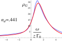
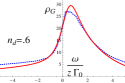
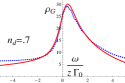
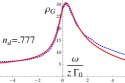
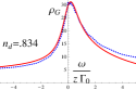
Figure 1: The spectral density for the physical Green’s function versus $\frac{\omega}{\Gamma_{0}z}$ for densities of $n_{d}=0.35,0.441,0.6,0.7,0.777,0.834$. The red curve is the ECFL calculation, while the blue curve is the NRG calculation.

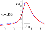
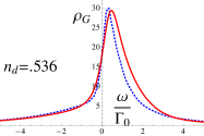
Figure 2: The spectral density for the physical Green’s function for the density of $n_{d}=0.536$. For the plot on the left, both the ECFL and NRG curves are plotted versus $\frac{\omega}{\Gamma_{0}z}$. Since ECFL has a larger z value, the absolute scale of the $\omega$ axis differs for the two curves. For the plot on the right, both ECFL and NRG are plotted versus $\frac{\omega}{\Gamma_{0}}$ and hence the ECFL peak is too wide.

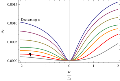
Figure 3: The spectral function for $\chi$ for densities of $n_{d}=0.834,0.777,0.7,0.6,0.536,0.441,0.35.$

Figure 4: The spectral function for $\Psi$ for densities of $n_{d}=0.834,0.777,0.7,0.6,0.536,0.441,0.35.$

In Fig. (5) we present the density evolution of the spectral function for the Dyson Mori self-energy (see Eq. (22)). This exhibits a remarkable similarity to the analogous spectral density for the  $t$-$J$  model in the limit of high dimensions Ref. (agcoll, ) and the Hubbard model at large $U$ Ref. (badmetal, ).

Figure 5: The spectral function for the Dyson-Mori self-energy for densities of $n_{d}=0.874,0.777,0.7,0.6,0.536,0.441,0.35.$ The curvature of the quadratic minimum becomes larger with increasing density.

IV Conclusion

In this work we have applied the ECFL formalism at the simplest level, using the $O(\lambda^{2})$ equations, to the Anderson impurity model with $U\rightarrow\infty$ . In this formalism, the two self-energies of the ECFL theory $\Psi$ and $\chi$ are calculated using a skeleton expansion in the auxiliary Green’s function ${\bf g}$. This is analogous to the skeleton expansion for the Dyson self-energy $\Sigma$, in standard Feynman-Dyson perturbation theory applicable to the case of finite $U$. These two self-energies determine ${\bf g}$ as well as the physical ${\cal{G}}$, leading to a self-consistent solution. We obtained the equations to second order and solved them numerically at $T=0$. We found that at low enough $\omega$, the ECFL self-energies have symmetric spectra of the type predicted by Fermi-Liquid theory (see Fig. (3) and Fig. (4)). Combining them through the ECFL functional form Eq. (22) generates a non-trivial self-energy with an asymmetric spectrum displayed in Fig. (5). It therefore appears that functional form Eq. (22) has the potential to generate realistic and non trivial spectral densities, starting with rather simple components. The availability of convenient and natural analytical expressions is seen to provide a distinct advantage of the ECFL formalism. Formally exact techniques such as the NRG involve steps that are not not automatically endowed with these, but rather rely on analytic continuation or other equivalent techniques.

The physical spectral function for the impurity site is obtained from the above pair of ECFL self energies, and displays a Kondo or Abrikosov-Suhl resonance. This feature becomes more narrow and the spectrum becomes more skewed towards the occupied side of the peak with increasing density. However, the computed quasiparticle $z$ in the present calculation is larger than the exact value, we comment further on this aspect below.

The location of the peak is set by $\epsilon_{d}+\Sigma_{DM}(0)$ (Eq. (21)). Using Eq. (41), we can see that this quantity must decrease with increasing density. This is consistent with our observation that the peak shifts to the left with increasing density. We expect that the location of the peak will approach $\omega=0$ as $n_{d}\rightarrow 1$. This can also be understood from the need to have more spectral weight to the left of $\omega=0$ to yield a higher value of $n_{d}$. We found that the ECFL spectrum satisfies the Friedel sum rule (Eq. (42)) to a high degree of accuracy, and that ECFL yields values of $\epsilon_{d}$ in good agreement with the NRG values at all densities (See Table (I).)

As mentioned above the ECFL calculation to $O(\lambda^{2})$ overestimates the value of the quasiparticle weight $z$ as compared with the NRG and the exact asymptotic result $z\propto e^{-1/2(1-n_{d})}$ as $n_{d}\to 1$ Ref. (rh84, ), the difference becoming more significant with increasing density. This also leads to an over broadening of the peak in the ECFL spectrum at higher densities. This is consistent with the fact that the $\lambda$ expansion of the ECFL is a low-density expansion and the current calculation has only been carried out to $O(\lambda^{2})$. Nevertheless, after rescaling the $\omega$ axis for both the ECFL and NRG spectra by their respective values of $z$, we find good quantitative agreement between the two as in Fig. (1). In Fig. (2) we illustrate the comparison between scaled and unscaled spectral functions at a typical density. We find similarly good agreement with the NRG calculation from Ref. (Costi, ).

Finally we note that the computed spectral functions exhibit a remarkable similarity to the analogous spectral density for the  $t$-$J$  model in the limit of high dimensions Ref. (agcoll, ) and the Hubbard model at large $U$ Ref. (badmetal, ).

V Acknowledgements

This work was supported by DOE under Grant No. FG02-06ER46319. We thank H. R. Krishnamurthy for helpful comments.

Appendix A Appendix A: Calculating the self-energies in the $O(\lambda^{2})$ theory

The calculation follows the procedure given in Ref. (Monster, ). A few comments are provided to make the connections explicit- the zeroeth order vertices are common to Ref. (Monster, ) Eqs. (B3, B14), and the first order ${\ \cal U}$ is common to Eq. (B15). The first order vertex $[\Lambda]_{1}$ can be found parallel to Eq-(B23- B28) from differentiating

$$[{\bf g}^{-1}(i,f)]_{1}=\Delta(i,f).{\bf g}^{(k)}(i,i)+\delta(i,f)\Delta(i,{{\mathbf{a}}}).{\bf g}^{(k)}({{\mathbf{a}}},f),$$ (51)

as

$$[\Lambda^{(a)}(i,m;j)]_{1}=-2\Delta(i,m).{\bf g}(i,j).{\bf g}(j,i)$$

$$-2\delta(i,m)\Delta(i,{{\mathbf{k}}}).{\bf g}({{\mathbf{k}}},j).{\bf g}(j,i).$$ (52)

Here the bold labels are integrated over. From this we construct the time domain self-energies

$$\Psi(i,f)=-2\lambda\Delta(i,{{\mathbf{k}}}).{\bf g}({{\mathbf{k}}},f).{\bf g}(i,f).{\bf g}(f,i),$$ (53)

and

$$\Phi(i,f)=-\delta(i,f)\Delta(i{{\mathbf{k}}}).{\bf g}({{\mathbf{k}}}i)$$

$$-2\lambda\Delta(i{{\mathbf{j}}}).{\bf g}({{\mathbf{j}}}{{\mathbf{k}}}).\Delta({{\mathbf{k}}}f).{\bf g}({{\mathbf{k}}}i).{\bf g}(i{{\mathbf{k}}})$$

$$-2\lambda\Delta(i{{\mathbf{j}}}).{\bf g}({{\mathbf{j}}}f).\Delta(f{{\mathbf{k}}}).{\bf g}({{\mathbf{k}}}i).{\bf g}(if).$$ (54)

After shifting $\Delta(i,f)\to\Delta(i,f)-\frac{u_{0}}{2}\delta(i,f)$ and Fourier transforming these we obtain Eq. (33) and Eq. (34). These expressions for the self-energies are correct to $O(\lambda)$ and lead to expression for ${\bf g}^{-1}$ and $\mu$ which are correct to $O(\lambda^{2})$. $\chi$ can be extracted from $\Phi$ as indicated in the text.

Appendix B Appendix B: Frequency summations

An efficient method to perform the frequency sums is to work with the time domain formulas Eq. (53) and Eq. (54) until the final step where Fourier transforms are taken. We note the representation for the Green’s function

$${\bf g}(\tau)=\int_{x}\rho_{\bf g}(x)e^{-\tau x}\left[\theta(-\tau)f(x)-\theta(\tau)\bar{f}(x)\right],$$ (55)

so that we can easily compound any pair that arises by dropping the cross products $\theta(\tau)\theta(-\tau)$ and using $\theta(\tau)^{2}=\theta(\tau)$. An example illustrates this procedure:

$${\bf g}(\tau){\bf g}(-\tau) = -\int_{x,y}\rho_{\bf g}(x)\rho_{\bf g}(y)e^{-\tau(x-y)}\times$$ (56)

$$\left[\theta(-\tau)f(x)\bar{f}(y)+\theta(\tau)\bar{f}(x)f(y)\right].$$

We also need to deal with the convolution of pairs of functions.

$$X(\tau) = \int_{-\beta}^{\beta}\ d\bar{\tau}\ {\bf g}(\bar{\tau})\left[\Delta(\tau-\bar{\tau})-\frac{u_{0}}{2}\delta(\tau-\bar{\tau})\right]$$ (57)

$$= \int_{x}\rho_{M}(x)e^{-\tau x}\left[\theta(-\tau)f(x)-\theta(\tau)\bar{f}(x)\right],$$

where the density $\rho_{M}(x)$ is defined in Eq. (49). This equation in turn is easiest to prove by transforming into a product in the Matsubara frequency space, simplifying using partial fractions, and then transforming back to time domain. We next note that Eq. (53) and Eq. (54) imply

$$\Psi(\tau) = -2\lambda\ X(\tau){\bf g}(\tau){\bf g}(-\tau),$$

$$\chi(\tau) = -2\lambda\ X(\tau)X(-\tau){\bf g}(\tau),$$ (58)

so that taking Fourier transforms is simplest if first multiply out as in Eq. (56), leading to Eq. (50).

References

- (1) B. S. Shastry, Phys. Rev. Letts. 107, 056403 (2011).
- (2) B. S. Shastry, Phys. Rev. B 87 125124 (2013); D. Hansen and B. S. Shastry, Phys. Rev. B 87, 245101 (2013).
- (3) Aficionados will recognize this as the case for the virial expansion in statistical mechanics, where a low density expansion can often be found for very strongly interacting systems. The critical density (where a phase transition occurs) is a natural boundary for such an expansion. If one knows a priori, that there is no critical density in a given problem such the Anderson model, then this expansion can be pushed to arbitrarily high densities. In the very different context of the theory of integrable systems in 1-dimension, this is precisely the reason why the asymptotic Bethe Ansatz works very well, even yielding exact results in regimes where its validity seems a-priori only approximate, as explained in Bill Sutherland, Beautiful Models, World Scientific Publishing Company, Singapore (2004).
- (4) P. W. Anderson, Phys. Rev. 124, 41 (1961).
- (5) P. W. Anderson, Phys. Rev. 164, 352 (1967); P. W. Anderson and G. Yuval, Phys. Rev. Lett. 23, 89 (1969).
- (6) F. D. M. Haldane, Phys. Rev. Letts. 40, 416 (1978).
- (7) K. G. Wilson, Rev. Mod. Phys. 47, 773 (1975).
- (8) H. R. Krishnamurthy, K. Wilson and J. Wilkins, Phys. Rev. B 21, 1003, 1044 (1980).
- (9) A.C. Hewson, A. Oguri, and D. Meyer, Eur. Phys. J. B. 40, 177 (2004); K. Edwards, A. C. Hewson, and V. Pandis, Phys. Rev. B 87, 165128 (2013).
- (10) D. E. Logan, M. P. Eastwood and M. A. Tusch, J. Phys. Condens. Matter 10, 2673 (1998)., M. T. Glossop and D. E. Logan J. Phys.: Condens. Matter 14 6737, (2002).
- (11) N. Bickers, Rev. Mod. Phys. 59, 845 939 (1987).
- (12) N. Read and D. M. Newns J. Phys. C 16, L1055 (1983); doi:10.1088/0022-3719/16/29/007; N. Read, J. Phys. C 18, 2651 (1985).
- (13) P. Coleman, Phys. Rev. B 29, 3035 (1984); S. E. Barnes, J. Phys. F 6 1375 (1976).
- (14) N. Andrei, Phys. Rev. Lett. 45, 379 (1980); P.B. Wiegmann, Sov. Phys. JETP Lett. 31, 392 (1980).
- (15) A. C. Hewson, The Kondo Problem to Heavy Fermions, Cambridge University Press, Cambridge (1993).
- (16) K. Yosida and K. Yamada, Prog. Theor. Phys. Suppl. 46, 244 (1970).
- (17) P. Nozières, J. Low. Temp. Phys. 17, 31 (1974).
- (18) A. C. Hewson, Phys. Rev. Letts. 70, 4007 (1993).
- (19) B. S. Shastry, arXiv:1110.1032 (2011), Phys. Rev. Letts. 109, 067004 (2012).
- (20) G.-H. Gweon, B. S. Shastry and G. D. Gu, arXiv:1104.2631 (2011), Phys. Rev. Letts. 107, 056404 (2011).
- (21) H. O. Frota and L. N. Olivera, Phys. Rev. B 33, 7871 (1986).
- (22) O. Sakai, Y. Shimuzu and T. Kasuya, J. Phys. Soc. Japan, 58, 162 (1989).
- (23) T. A. Costi and A. C. Hewson, J.. Phys. Cond. Matter, L 361 (1993).
- (24) T. A. Costi, J. Kroha, and P. Wölfle, Phys. Rev. B 53, 1850 (1996). We thank the authors for providing us with the digital versions of their results.
- (25) In the notation of Ref. (ECFL, ) Eq. (58), this corresponds to writing .
- (26) “Extremely Correlated Fermi Liquids in the limit of infinite dimensions”, E. Perepelitsky and B. S. Shastry, to be published (2013).
- (27) J. Friedel, Can. Jour. Phys. 54, 1190 (1956)
- (28) J. S. Langer and V. Ambegaokar, Phys. Rev. 164, 498 (1961).
- (29) D. C. Langreth, Phys. Rev. 150, 516 (1966).
- (30) J. M. Luttinger and J. C. Ward, Phys. Rev. 118, 1417 (1960).
- (31) J. W. Rasul and A. C. Hewson, J. Phys. C: Solid State Phys. 17, 3337 (1984).
- (32) To recover Eq. (42), we may use Eq. (21) and the Fermi liquid assumption of so that and combine with Eq. (41).
- (33) D. Hansen, Jernej Mravlje , E. Perepelitsky, Rok Zitko, A. Georges and B. S. Shastry, to be published (2013).
- (34) X. Deng, J. Mravlje, R. Z itko, M. Ferrero, G. Kotliar, and A. Georges, Phys. Rev. Letts. 110, 086401 (2013)